2014 14th International Conference on Control, Automation and Systems (ICCAS 2014)Oct. 22–25, 2014 in KINTEX, Gyeonggi-do, Korea

Controlling an Overactuated Vehicle with Application to an AutonomousSurface Vehicle Utilizing Azimuth Thrusters

Darsan Patel1, Daniel Frank2, and Dr. Carl Crane3

1Department of Mechanical Engineering, University of Florida,Gainesville, Florida (darsan1313@gmail.com)

2Department of Mechanical Engineering, University of Florida,Gainesville, Florida (dzf209@gmail.com)

3Department of Mechanical Engineering, University of Florida,Gainesville, Florida (carl.crane@gmail.com)

Abstract: A control algorithm for allocating control effort to a generic overactuated system is designed. In the casewhere redundant actuators in the system allow for an infinite number of possible solutions to a desired trajectory, thecontroller must decide which solution to take. A PD controller is implemented to solve for the desired force and momentof the trajectory. Once the forces and the moments are acquired, a cost function is utilized to help guide the choice of theactuator configuration. This control method is then validated through the simulation of an autonomous surface vehiclethat is utilizing an azimuth thruster propulsion system.

Keywords: Control Allocation, Overactuated Systems, Azimuth Thruster, Autonomous Surface Vehicle

1. INTRODUCTIONIn many applications it is desirable to design an over-

actuated system, that is, a system that has more inputsthan outputs. One of the major advantages of this type ofsystem is that the redundancy may allow the system to bemore robust in the case of actuator failure. If an actua-tor stops working in an overactuated system, it may stillbe possible for the system to achieve full mobility. Thedownside to this is that the addition of redundant actu-ators accounts to traditionally undesirable traits such asadditional weight, fuel costs, system complexity, etc. Re-dundant actuators also create an interesting challenge forthe designer of the controller. There may no longer bea unique input to the controller that can achieve the de-sired output. Instead, there may be a set of possible solu-tions or even an infinite number of solutions. In order forthe controller to function properly in this type of system,it needs an algorithm to help it decide which solution ismost suited to obtain the desired output.

One example of an overactuated system is the Sub-juGator, an autonomous underwater vehicle (AUV) [1].It features eight thrusters to help control its six degreesof freedom while underwater as shown in Fig. 1. TheAUV is designed so that if any thruster fails, it may stillachieve full mobility. There are even certain combina-tions of two thrusters that may fail without it affectingthe AUV’s ability to control its six degrees of freedom inthe water. The nonlinear controller utilized on the AUVfeatures a robust integral of the sign of the error feed-back term with a neural network based feedforward termin order to achieve semi-global asymptotic tracking withthe presence of complete model uncertainty and unknowndisturbances [2], [3]. The controller has been validatedwith both simulated and experimental results.

Fig. 1 Overactuated AUV with illustrated thrust vectors

There are a variety of methods that researchers haveimplemented in order to deal with the issue of multiplepossible solutions. One algorithm that was developedto solve this challenge utilizes the Karush-Kuhn-Tuckerconditions [4]. This method was simulated on an elec-tric ground vehicle actuated by in-wheel motors. A con-tinuation of this study, which included experimental re-sults, incorporated the efficiency functions and workingmodes of redundant actuators in order to reduce the over-all power consumption of the system [5]. In [6], [7],model predictive control allocation was used with modelreference control to achieve control of an overactuatedsystem where the actuators had different dynamic author-ities and saturation limits. The controller was validatedby both simulations and experimental results. Fuzzylogic was used in [8] to adaptively change the gains ofthe control allocution. In [9], two methods for controlallocution to an overactuated system are presented. Thefirst approach involved an H∞ controller designed usinglinear matrix inequalities. The second approach uses an

adaptive weight updating algorithm.To validate the controller developed in this paper, a

simulation will be performed on an autonomous surfacevehicle (ASV) that utilizes an azimuth thruster propulsionsystem, shown in Fig. 2. An azimuth thruster is simply amarine propeller that can be rotated horizontally to assistin steering. Since the propulsion devices are steerable,the interaction of closely positioned actuators can havean impact on the overall behavior and efficiency of thesystem. The interaction of multiple azimuth thrusters wasconsidered in [10]. However, due to the difficult nature ofmodeling these interactions, they will not be consideredin the simulation, but may be included in future work.

Fig. 2 CAD model of the simulated azimuth thruster

2. CONTROL ALGORITHMFor the purposes of this paper, it is assumed that the

system to be controlled:• Can be actuated• Spans over all degrees of freedom• Full model knowledge is availableThe controller, which in this case is simply a PD con-troller, maps the error of the position and orientation tothe required magnitude and direction of the force and themoment. A block diagram of the control configurationcan be seen in Fig. 3.

The product of the controller, the control input, is apure force and moment acting on the center of mass ofa simplified system. Therefore, the controller must betuned with a simplified model of the system. The simpli-fied model is a rigid body with mass and moment of iner-tia of the system being manipulated in space with a pureforce and moment vector acting on the center of mass ofthe system. A block diagram of the controller operatingon the simplified system can be seen in Fig. 4.

The cost function minimizer maps the required forceand moment acquired by the controller to the most costeffective actuator orientation for the system to reach thegiven force and moment. The cost function is composedof different variables such as error, energy consumption,

Fig. 3 Block diagram of the control configuration

Fig. 4 Block diagram of the simplified system

time to reach desired state of the actuator, etc. The costfunction is minimized to get the most cost effective solu-tion or actuator configuration. There are several ways tominimize the cost function: discrete point evaluation, thesteepest descent method, Newton’s method, and combi-nations of the above [11].

3. SIMULATION MODEL

The validity of the controller will be simulated on anASV utilizing an azimuth thruster steering system. Theboat features two trolling motors attached to the stern ofthe vehicle that can be independently positioned. Thesteering motors are modeled after Dynamixel MX- 64Tservo motors with a maximum speed of 78 RPM . Thesteering motors and propulsion motors are attached viatiming pulleys and a timing belt with a total gear reduc-tion of 1:1. In this simulation, the trolling motors areassumed to be capable of producing a maximum thrust of100 N .

3.1 System DynamicsIn order to describe the dynamics of the system, two

reference frames are defined; Let E be a reference framefixed to ground.

Ex = to the rightEz = out of the pageEy = Ez × Ex

The boat reference frame e, is fixed to the rigid body ofthe boat with an origin at the boat’s center of mass.

ex = toward starboardez = Ez

ey = ez × ex

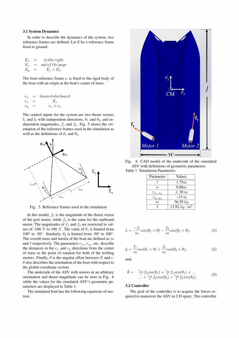
The control inputs for the system are two thrust vectorsf1 and f2 with independent directions, θ1 and θ2, and in-dependent magnitudes, f1 and f2. Fig. 5 shows the ori-entation of the reference frames used in the simulation aswell as the definitions of θ1 and θ2.

Fig. 5 Reference frames used in the simulation

In this model, f1 is the magnitude of the thrust vectorof the port motor, while f2 is the same for the starboardmotor. The magnitudes of f1 and f2 are restricted to val-ues of -100 N to 100 N . The value of θ1 is limited from100° to -50°. Similarly, θ2 is limited from -50° to 100°.The overall mass and inertia of the boat are defined as mand I respectively. The parameters rx1 , ry1 , etc. describethe distances in the ex and ey directions from the centerof mass to the point of rotation for both of the trollingmotors. Finally, θ is the angular offset between E and e.θ also describes the orientation of the boat with respect tothe global coordinate system.

The underside of the ASV with motors in an arbitraryorientation and thrust magnitude can be seen in Fig. 6while the values for the simulated ASV’s geometric pa-rameters are displayed in Table 1.

The simulated boat has the following equations of mo-tion,

Fig. 6 CAD model of the underside of the simulatedASV with definitions of geometric parameters

Table 1 Simulation ParametersParameter Values

l 1.75mw 0.86m

rx1,x2 ±.30 mry1,y2 -.15 mm 36.29 kgI 13.92 kg ·m2

x =−f1m

sin(θ1 + θ)− f2m

sin(θ2 + θ), (1)

y =f1m

cos(θ1 + θ) +f2m

cos(θ2 + θ), (2)

and,

θ =rx1

I f1cos(θ1) +ry1I f1sin(θ1) + . . .

. . .+rx2

I f2cos(θ2) +ry2I f2sin(θ2).

(3)

3.2 ControllerThe goal of the controller is to acquire the forces re-

quired to maneuver the ASV in 2-D space. The controller

maps the error between the global position, velocity, ori-entation, and angular velocity of the vehicle with the ref-erence global position, velocity, orientation, and angularvelocity to the required force and moment,

controller :

exexeyeyeθeθ

=

x− xref

x− xref

y − yrefy − yrefθ − θrefθ − θref

→

fxreqfyreqmzreq

.

The required forces are designed as follows,

fxreqfyreqmzreq

=

kx1ex + kx2 exky1ey + ky2 eykθ1eθ + kθ2 eθ

, (4)

which is essentially a PD controller.

3.2.1 Tuning GainsEq. (4) can be decoupled into three separate systems

as shown in Eq. (5),

u =

kx1 kx2 0 0 0 00 0 ky1 ky2 0 00 0 0 0 kθ1 kθ2

exexeyeyeθeθ

. (5)

The full model of the system can be simplified to forcesacting on a rigid body as mentioned in section 2. Us-ing Newton’s second law, the simplified system is repre-sented as:

fx = mxfy = mymz = Iθ.

This can also be represented in state space form,

v = Av +Bu,

where,

A =

0 1 0 0 0 00 0 0 0 0 00 0 0 1 0 00 0 0 0 0 00 0 0 0 0 10 0 0 0 0 0

,

is the system matrix,

B =

0 0 01m 0 00 0 00 1

m 00 0 00 0 1

I

,

is the input matrix,

v =

xxyyθ

θ

,

is the state vector and,

u =

fxfymz

,

is the input vector. The method of pole placement canbe used to solve for the gains of the controller which areshown in Table 2.Table 2 Simulation Gains

Gain Valueskx1 50kx2 85.1908ky1 50ky2 85.1908kθ1 70kθ2 45.7105

3.3 Optimization Using a Cost FunctionThe cost function minimizer maps required force and

moment to an actuator configuration,

minimizer :

fxreqfyreqmzreq

→

θ1f1θ2f2

.

The actuator configurations are obtained by minimizingthe cost function as mentioned in section 2.

θ1f1θ2f2

=

argθ1f1θ2f2

∈

min100° → −50°

−100N → 100N−50° → 100°

−100N → 100N

V,

where,

12k1(efx)

2 + 12k2(efy)

2 + . . .V = . . . 1

2k3(emz)2 + 1

2k4(f1)2 + . . .

. . . 12k5(f2)

2 + 12k6(θ1)

2 + 12k7(θ1)

2,(6)

efx = fx − fxrefefy = fy − fyrefemz = mz −mzref ,

and the cost function gains are defined in Table 3. Thecost function gains are determined by the performancethat the user requires of the ASV. For example, if the userdesires very accurate positioning without regard to fuelcosts, they would weigh k1 and k2 more heavily than k4and k5.Table 3 Cost Function Gains

Gain Description Valuesk1 force error in x-direction 1000k2 force error in y-direction 1000k3 moment error 1000k4 port energy 10k5 starboard energy 10k6 variation in θ1 1k7 variation in θ2 1

The cost function contains the error between the re-quired force acquired by the controller from section 3.2and the force output from the modeled system. Thismodel maps the actuator configuration to the expectedforce.

model :

θ1f1θ2f2

→

fxfymz

,

fx = −f1s1 − f2s2fy = f1c1 + f2c2mz = rx1f1c1 + ry1f1s1 + rx2f2c2 + ry2f2s2,

(7)

where,

s1,2 = sin(θ1,2)c1,2 = cos(θ1,2).

The advantage of placing f1 and f2 into the cost func-tion is to penalize high energy consumption. Similarly,placing θ1 and θ2 into the cost function helps minimizeenergy consumption as well as strain on the actuators.

To minimize the cost function, a brute force approachwas used. The cost function is evaluated 160k timeswith different combinations of actuator efforts. All of the

evaluations were compared and the effort with the low-est associated cost was assumed to be the solution at thatpoint in time. While this method ensures that the cho-sen actuator configuration minimizes the cost function, itis slow compared to other numerical algorithms such asconstrained nonlinear optimization or Newton’s method.Assuming a 2MHz processor, the loop time using thismethod is approximately .5 Hz. In order for the actualASV to perform properly, the motors will require an up-date speed of approximately 20 Hz. One way to speedup the controller is to calculate all possible outputs for agiven set of inputs offline and put them in a lookup table.While this method is faster, it requires a very accurate un-derstanding of the system dynamics in order for it to beeffective.

4. SIMULATION RESULTSThe simulation in this study was performed on MAT-

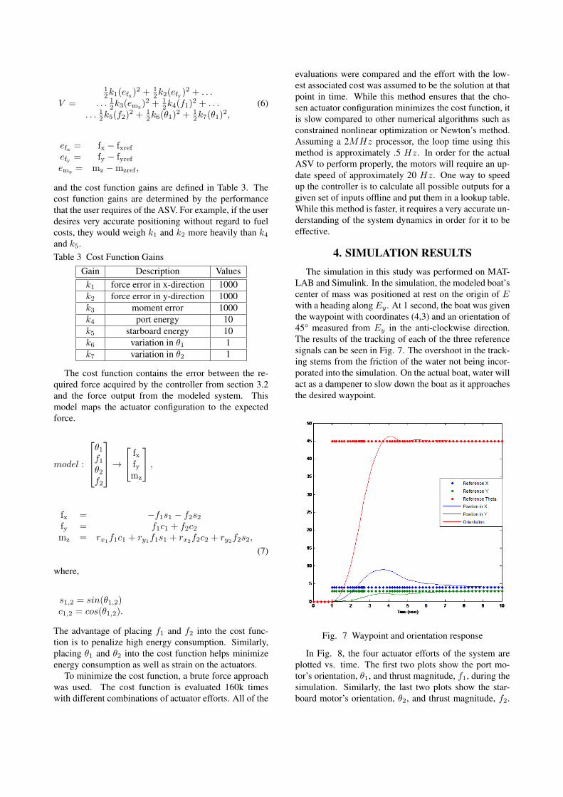
LAB and Simulink. In the simulation, the modeled boat’scenter of mass was positioned at rest on the origin of Ewith a heading along Ey . At 1 second, the boat was giventhe waypoint with coordinates (4,3) and an orientation of45° measured from Ey in the anti-clockwise direction.The results of the tracking of each of the three referencesignals can be seen in Fig. 7. The overshoot in the track-ing stems from the friction of the water not being incor-porated into the simulation. On the actual boat, water willact as a dampener to slow down the boat as it approachesthe desired waypoint.

Response.eps

Fig. 7 Waypoint and orientation response

In Fig. 8, the four actuator efforts of the system areplotted vs. time. The first two plots show the port mo-tor’s orientation, θ1, and thrust magnitude, f1, during thesimulation. Similarly, the last two plots show the star-board motor’s orientation, θ2, and thrust magnitude, f2.

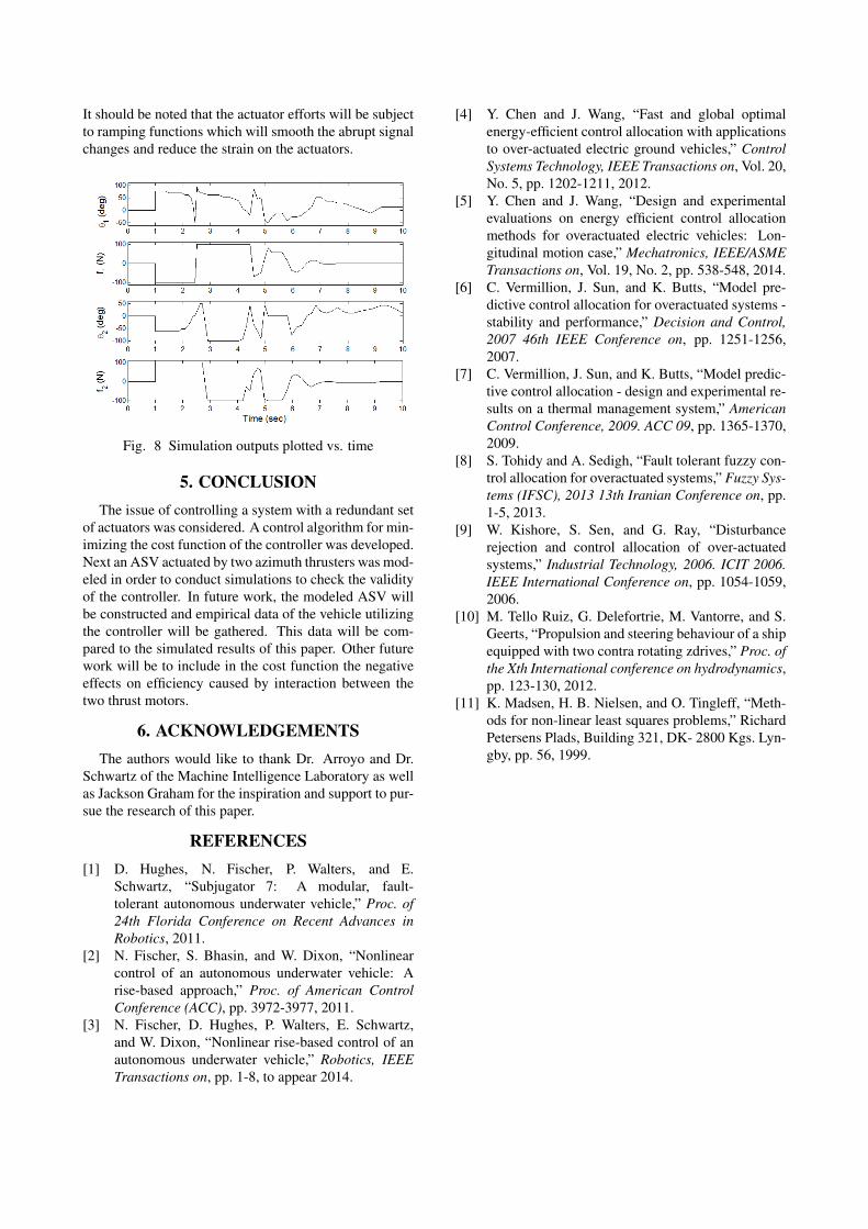
It should be noted that the actuator efforts will be subjectto ramping functions which will smooth the abrupt signalchanges and reduce the strain on the actuators.

Fig. 8 Simulation outputs plotted vs. time

5. CONCLUSIONThe issue of controlling a system with a redundant set

of actuators was considered. A control algorithm for min-imizing the cost function of the controller was developed.Next an ASV actuated by two azimuth thrusters was mod-eled in order to conduct simulations to check the validityof the controller. In future work, the modeled ASV willbe constructed and empirical data of the vehicle utilizingthe controller will be gathered. This data will be com-pared to the simulated results of this paper. Other futurework will be to include in the cost function the negativeeffects on efficiency caused by interaction between thetwo thrust motors.

6. ACKNOWLEDGEMENTSThe authors would like to thank Dr. Arroyo and Dr.

Schwartz of the Machine Intelligence Laboratory as wellas Jackson Graham for the inspiration and support to pur-sue the research of this paper.

REFERENCES[1] D. Hughes, N. Fischer, P. Walters, and E.

Schwartz, “Subjugator 7: A modular, fault-tolerant autonomous underwater vehicle,” Proc. of24th Florida Conference on Recent Advances inRobotics, 2011.

[2] N. Fischer, S. Bhasin, and W. Dixon, “Nonlinearcontrol of an autonomous underwater vehicle: Arise-based approach,” Proc. of American ControlConference (ACC), pp. 3972-3977, 2011.

[3] N. Fischer, D. Hughes, P. Walters, E. Schwartz,and W. Dixon, “Nonlinear rise-based control of anautonomous underwater vehicle,” Robotics, IEEETransactions on, pp. 1-8, to appear 2014.

[4] Y. Chen and J. Wang, “Fast and global optimalenergy-efficient control allocation with applicationsto over-actuated electric ground vehicles,” ControlSystems Technology, IEEE Transactions on, Vol. 20,No. 5, pp. 1202-1211, 2012.

[5] Y. Chen and J. Wang, “Design and experimentalevaluations on energy efficient control allocationmethods for overactuated electric vehicles: Lon-gitudinal motion case,” Mechatronics, IEEE/ASMETransactions on, Vol. 19, No. 2, pp. 538-548, 2014.

[6] C. Vermillion, J. Sun, and K. Butts, “Model pre-dictive control allocation for overactuated systems -stability and performance,” Decision and Control,2007 46th IEEE Conference on, pp. 1251-1256,2007.

[7] C. Vermillion, J. Sun, and K. Butts, “Model predic-tive control allocation - design and experimental re-sults on a thermal management system,” AmericanControl Conference, 2009. ACC 09, pp. 1365-1370,2009.

[8] S. Tohidy and A. Sedigh, “Fault tolerant fuzzy con-trol allocation for overactuated systems,” Fuzzy Sys-tems (IFSC), 2013 13th Iranian Conference on, pp.1-5, 2013.

[9] W. Kishore, S. Sen, and G. Ray, “Disturbancerejection and control allocation of over-actuatedsystems,” Industrial Technology, 2006. ICIT 2006.IEEE International Conference on, pp. 1054-1059,2006.

[10] M. Tello Ruiz, G. Delefortrie, M. Vantorre, and S.Geerts, “Propulsion and steering behaviour of a shipequipped with two contra rotating zdrives,” Proc. ofthe Xth International conference on hydrodynamics,pp. 123-130, 2012.

[11] K. Madsen, H. B. Nielsen, and O. Tingleff, “Meth-ods for non-linear least squares problems,” RichardPetersens Plads, Building 321, DK- 2800 Kgs. Lyn-gby, pp. 56, 1999.