convection in white dwarf stars
TRANSCRIPT
Convection in White Dwarf Stars
Kevin J. P. Luecke
Table of Contents
1 Introduction 2
2 Turbulent energy transport 2
2.1 Condition for Convection . . . . . . . . . . . . . . . . . . . . . . . . . . . . . 3
2.2 Mixing Length Theory . . . . . . . . . . . . . . . . . . . . . . . . . . . . . . 6
2.3 Antares . . . . . . . . . . . . . . . . . . . . . . . . . . . . . . . . . . . . . . 7
3 Interaction Between Convection and Pulsations 9
3.1 Lcfit theta and GAMA . . . . . . . . . . . . . . . . . . . . . . . . . . . . . . 11
3.1.1 Description of GPU Implementation . . . . . . . . . . . . . . . . . . 12
3.2 Wu’s Approximation . . . . . . . . . . . . . . . . . . . . . . . . . . . . . . . 13
4 Targets and Data Acquisition 14
4.1 HS0507 . . . . . . . . . . . . . . . . . . . . . . . . . . . . . . . . . . . . . . 14
4.2 Instrumentation . . . . . . . . . . . . . . . . . . . . . . . . . . . . . . . . . . 15
5 Data Analysis 16
6 Remaining work 17
7 Bibliography 17
Convection in White Dwarf Stars Kevin Luecke
1. Introduction
White dwarfs are some of the simplest stars. Because of their simplicity, they can be
studied to learn fundamental facts about the universe. By studying them, we can learn about
their progenitors, and 97% of stars end their lives a white dwarfs. They can also be used
to find the age of the galactic disc. These determinations, however, rely on the accuracy of
our models of white dwarfs. In white dwarf science and the field of Astrophysics in general,
one of the most prevalent, and least understood phenomena is convection. The reason for
this uncertainty is the non-local nature of convection. One could argue that the beginning
of modern science, (certainly classical physics) came with Newton and the development of
calculus. Calculus is the system we use to describe change, and has been widely applied
across the sciences. However, this technique, while incredibly useful, cannot describe non-
local phenomena, or situations where any point can be effected by far off points. Convection
is just such a situation. Because you can’t break these problems down to a simple, local
approximation, we have no analytical tools to solve them. These kind of problems went
largely unsolved until recently.
With the advent of the computer came the hope of computing the effects of convective
regions directly from first principals. Unfortunately, to compute the effects exactly you
need an unattainable amount of computational power. By making some assumptions and
simplifications, however, you can bring the problem into a regime which is computable by
modern, massively parallel computers. This kind of simulation has been achieved in many
stars, most notably the sun [cite]. To confirm the accuracy of these solar simulations data
from luminosity variations along the surface can be used. For other stars, however, no
such spatial resolution is possible, so some other effect of convection must be measured.
Fortunately, pulsations in certain classes of white dwarfs interact with convection giving us
just such an effect. By fitting models of stars with these two interacting phenomena to data
from real stars, we can learn more about convection in the physical regime of white dwarfs,
as well as about the white dwarfs themselves.
2. Turbulent energy transport
Turbulent energy transport, or convection occurs in most stars, including our sun. It
even occurs in planets like the earth. Understanding convection better can help us un-
derstand all the stars and even possibly earth weather. To be able to parametrize this
phenomena, we have to first understand why it happens.
– 2 –
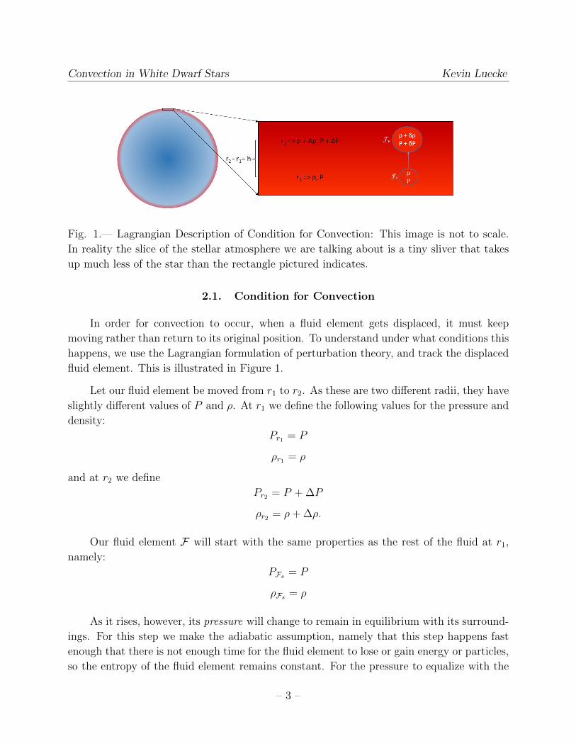
Convection in White Dwarf Stars Kevin Luecke
Fig. 1.— Lagrangian Description of Condition for Convection: This image is not to scale.
In reality the slice of the stellar atmosphere we are talking about is a tiny sliver that takes
up much less of the star than the rectangle pictured indicates.
2.1. Condition for Convection
In order for convection to occur, when a fluid element gets displaced, it must keep
moving rather than return to its original position. To understand under what conditions this
happens, we use the Lagrangian formulation of perturbation theory, and track the displaced
fluid element. This is illustrated in Figure 1.
Let our fluid element be moved from r1 to r2. As these are two different radii, they have
slightly different values of P and ρ. At r1 we define the following values for the pressure and
density:
Pr1 = P
ρr1 = ρ
and at r2 we define
Pr2 = P + ∆P
ρr2 = ρ+ ∆ρ.
Our fluid element F will start with the same properties as the rest of the fluid at r1,
namely:
PFs = P
ρFs = ρ
As it rises, however, its pressure will change to remain in equilibrium with its surround-
ings. For this step we make the adiabatic assumption, namely that this step happens fast
enough that there is not enough time for the fluid element to lose or gain energy or particles,
so the entropy of the fluid element remains constant. For the pressure to equalize with the
– 3 –
Convection in White Dwarf Stars Kevin Luecke
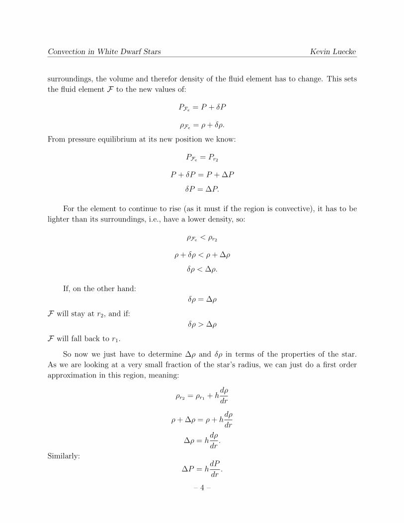
surroundings, the volume and therefor density of the fluid element has to change. This sets
the fluid element F to the new values of:
PFe = P + δP
ρFe = ρ+ δρ.
From pressure equilibrium at its new position we know:
PFe = Pr2
P + δP = P + ∆P
δP = ∆P.
For the element to continue to rise (as it must if the region is convective), it has to be
lighter than its surroundings, i.e., have a lower density, so:
ρFe < ρr2
ρ+ δρ < ρ+ ∆ρ
δρ < ∆ρ.
If, on the other hand:
δρ = ∆ρ
F will stay at r2, and if:
δρ > ∆ρ
F will fall back to r1.
So now we just have to determine ∆ρ and δρ in terms of the properties of the star.
As we are looking at a very small fraction of the star’s radius, we can just do a first order
approximation in this region, meaning:
ρr2 = ρr1 + hdρ
dr
ρ+ ∆ρ = ρ+ hdρ
dr
∆ρ = hdρ
dr.
Similarly:
∆P = hdP
dr.
– 4 –
Convection in White Dwarf Stars Kevin Luecke
To find δρ, we have to know how ρ changes as a function of P , with the entropy held
fixed. This is known as the equation of state. In general, we can write the equation of state
in this form:
ρ = ρ(P, S).
Here ρ is a function of pressure and entropy, however, in our fluid element, the entropy does
not have time to change so:
ρFe = ρ(Pr2 , Sr1) = ρ(P + ∆P, S)
Expanding around ρ(P, S) we have
ρFe = ρ(P, S) + ∆P
(∂ρ
∂P
)S
+ ∆S
(∂ρ
∂S
)P
,
and since the entropy is constant (∆S = 0), this yields
ρFe = ρ(P, S) + ∆P
(∂ρ
∂P
)S
ρ+ δρ = ρ+ hdP
dr
(∂ρ
∂P
)S
δρ = hdP
dr
(∂ρ
∂P
)S
.
So the condition for convection to occur is:
δρ < ∆ρ
hdP
dr
(∂ρ
∂P
)S
< hdρ
dr
dP
dr
(∂ρ
∂P
)S
<dρ
dr.
The dPdr
and dρdr
terms are the changes in pressure and density respectively as we get
farther out in the star. The pressure and density decrease from the center to the surface, so
we can saydP
dr< 0
dρ
dr< 0
– 5 –
Convection in White Dwarf Stars Kevin Luecke
This means I can rearrange the inequality as given below:(∂ρ
∂P
)S
>
(dρdr
)(dPdr
) =dρ
dP.
So in order for convection to occur, the local change in density with pressure in a region of
the star has to be less than the adiabatic change in density with pressure. It is important
to note that if we were to do a similar derivation for a fluid element displaced downwards
towards the center of the star, that continued to sink, we would obtain the same result.
2.2. Mixing Length Theory
From the derivation above, we can conclude that convection does occur, and indeed it
occurs somewhere in most stars. However, at this point our ability to interpret convection
analytically ends. When these displaced fluid elements are lighter than the surrounding fluid,
they speed up and continue to rise. This acceleration continues throughout the region of the
star where the condition I derived above remains true. This makes it very hard to figure out
what actually happens in these regions. If fluid elements can slam through a region changing
the local conditions abruptly, it is hard to rely on any assumptions about local stability that
lie at the heart of calculus.
Even following just one fluid element and keeping the rest fixed can lead to problems. If
the fluid element keeps accelerating, minor differences in the density or pressure of the fluid
through which it’s moving can deflect or slow it, breaking it up unpredictably. Because of
this, convection remains a largely unsolved problem today and one of the largest sources of
uncertainty in stellar modeling (Montgomery 2005).
Currently, the most commonly used approximation of convection is known as Mixing
Length Theory. This method is only an order of magnitude approximation, and is used
because it is easy to compute rather than because of any faith in its accuracy. As Kippenhahn
says, “we do not believe it [mixing-length theory] to be sufficient, but it does provide at least
a simple method for treating convection locally at any given point of a star.” (Kippenhahn
book “Stellar Evolution”) Basically, mixing-length theory assumes that convection happens
over a certain length lm (the “mixing length”) and from there derives an equation for the
energy flux through that section of the star. With this, most other properties of the star
important to stellar evolution can be determined.
However, the correct value for lm is not readily apparent. The normal ad hoc assumption
is that the mixing length is some parameter α, which is of order 1, times the local pressure
– 6 –
Convection in White Dwarf Stars Kevin Luecke
scale height, i.e.,
lm = αHP ,
where
HP = − P
dP/dr.
This parameter α varies widely between different types of stars, which drastically reduces
its predictive power. Fortunately with the power of the TACC (Texas Advanced Computing
Center) and other super computers, a more complete treatment of this problem can be
attained.
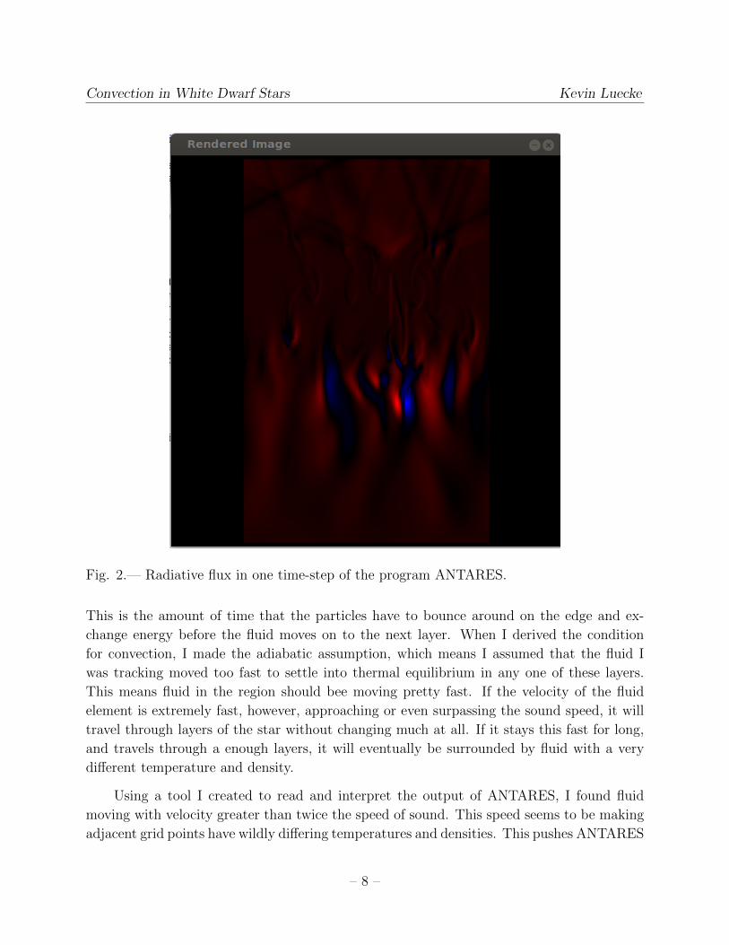
2.3. Antares
In order to better define the size and properties of the convection region of white dwarfs,
I have attempted to simulate this convective region of the star. Hydrodynamic simulations
take an Eulerian approach to fluid dynamics, breaking up the convective region into a grid of
points each with their own values for ρ, P , T , and many other physical properties of matter.
This simulation continuously updates these physical properties for each grid point after short
time intervals based on the properties of the points around them. To figure out how to update
each grid-point, the simulation relies on tables of measured equation of state relationships.
This process of updating the grid-points relies only on basic principals of physics, so it’s
reliable, but computationally expensive. Getting it to complete in a realistic time frame
requires a lot of algorithm refinement and optimization that balances speed with accuracy.
The program I have used for this simulation is the ANTARES program, developed at the
University of Vienna to simulate the convective region of the sun. I created a program to
visualize this output. A sample rendering is shown in Figure 2. This program has had great
success when applied to the sun and A-Stars, and is now being applied to large, Jupiter-like
planets. However, in the case of white dwarfs, I have run into some difficulties that appear
to be caused by extremely fast moving fluid elements.
There are two speeds that are important in this simulation, the speed of the fluid
element, and the sound speed. The sound speed is important because it controls the speed
at which thermal equilibrium is reached. If we picture the star as a set of discrete layers,
each with its own pressure, density, and temperature, a fluid element passing through these
layers spends a discrete amount of time in each
trn =h
v F.
– 7 –
Convection in White Dwarf Stars Kevin Luecke
Fig. 2.— Radiative flux in one time-step of the program ANTARES.
This is the amount of time that the particles have to bounce around on the edge and ex-
change energy before the fluid moves on to the next layer. When I derived the condition
for convection, I made the adiabatic assumption, which means I assumed that the fluid I
was tracking moved too fast to settle into thermal equilibrium in any one of these layers.
This means fluid in the region should bee moving pretty fast. If the velocity of the fluid
element is extremely fast, however, approaching or even surpassing the sound speed, it will
travel through layers of the star without changing much at all. If it stays this fast for long,
and travels through a enough layers, it will eventually be surrounded by fluid with a very
different temperature and density.
Using a tool I created to read and interpret the output of ANTARES, I found fluid
moving with velocity greater than twice the speed of sound. This speed seems to be making
adjacent grid points have wildly differing temperatures and densities. This pushes ANTARES
– 8 –
Convection in White Dwarf Stars Kevin Luecke
equation of state lookups into regimes we haven’t measured yet. Unable to resolve these
gridpoints, the simulation ends before producing useful results. I have been unable to find a
way to resolve this problem and leave it to future work.
3. Interaction Between Convection and Pulsations
Concurrently with the ANTARES project, I have been building on the work of my
adviser Mike Montgomery. In his 2005 paper entitled “A New Technique for Probing Con-
vection in Pulsating White Dwarf Stars”, Montgomery builds on the work of Brickhill and
that of Goldreich & Wu, in developing a technique to measure convection zone size by fitting
observations. In this section I will follow this derivation. This technique takes advantage
of the extreme oscillations in the physical properties of the atmospheres of pulsating white
dwarfs.
As part of their evolutionary cycle, white dwarfs with hydrogen atmospheres (DAs)
enter what is known as the instability strip, where they can change in brightness by 10%
in a matter of minutes, as pictured in Figure 4. These brightness variations are a result of
harmonic oscillations in temperature and density throughout the star. These variations in
brightness (or energy flux), then should be described by standard harmonic oscillations of a
spherical object:
F =∑j
Re[Ajei(ωjt+δj)Ylj ,mj
(θ, φ)].
Here the characteristic sinusoidal behavior of a wave is represented by Ajei(ωjt+δj), each of
the j waves, has an amplitude A, a frequency ω, and a phase δ. The effects of the spherical
structure of the star are taken into account through Lapace’s spherical harmonic equations,
Yl,m(θ, φ), where θ and φ are spherical coordinates, and l and m are integers such that
−l < m < l. This fits our observations fairly well, however the light curves show additional
nonlinear effects. These effects have long been attributed to convection ?. As a star pulsates,
the fundamental physical parameters of the star (e.g., its temperature and density) change.
When these parameters change, so does the size of its convective envelope.
Three facts about these stars make it possible to parametrize this constantly changing
convection zone. First of all, the time it takes a convection zone to relax into stable state
(convective turnover timescale) is much less than the time is takes a pulsation to complete
a cycle. Secondly, the radial size of the convection zone is much smaller than the radial
wavelength of a pulsation. This means at any given time we can assume the the convection
zone on any section of the surface of the star is the same as a convection zone of a non-
pulsating star in equilibrium at that temperature. Finally, as the convective envelope lies on
– 9 –
Convection in White Dwarf Stars Kevin Luecke
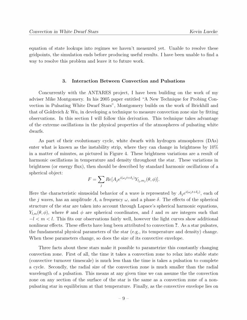
Fig. 3.— Value of the convective turnover timescale as a function of effective temperature
as predicted by mixing length theory. A few different values of α that are appropriate for
white dwarfs have been plotted.
the very outer edge of the star, we can assume that the energy flux underneath the convection
zone strictly follows the equation above.
As a fluid becomes convective its method of energy transport changes, which can be
thought of like a phase change. This means the energy flux leaving the star is the flux
entering the convective region minus the energy it takes to “change the phase” of fluid
elements from convective to non-convective:
Fphot = Fbase − τCdFphotdt
,
where τC is the convective turnover timescale and can be thought of as the heat capacity
of the convection zone. The formula for the flux at the base is the standard model for
white dwarfs mentioned earlier. Using mixing length theory, we can estimate the convective
timescale as a function of temperature. Even if you vary the mixing length parameter α, τCis fitted by a power of Teff . To see this more clearly we can plot log(τC(Teff)), and notice
that it is nearly linear, with a negative slope (see Figure 3). From this we can approximate
the convective timescale:
τC(Teff) ≈ τ0 ×(Teff
Teff,0
)−NHere Teff,0 is the starting temperature, τ0 is a constant depending on α, and N is a constant
approximately between 90 and 95 in DAs. This supports the theory that τC is strongly
dependent on T , and the convection zone strongly effects the energy flux at the photosphere
(Fphot).
– 10 –
Convection in White Dwarf Stars Kevin Luecke
Using this model as the basis for a fitting program, Montgomery has been able to
reproduce the light curves of simple stars with extreme accuracy. However, this program is
not able to fit all of the parameters quickly enough to be useful on complex stars. To fix
this problem, I have expanded the program to take advantage of massively parallel hardware
on personal computers as well as that available to University of Texas students through the
Texas Advanced Computing Center (TACC).
3.1. Lcfit theta and GAMA
The program Montgomery wrote fit effects of convection zones on light curves is called
Lcfit theta. This program solves the following ordinary differential equation (ODE), repro-
duced in full:
Fphot = −
[τ0 ×
(Teff
Teff,0
)−N]dFphotdt
+∑j
Re[Ajei(ωjt+δj)Ylj ,mj
(θ, φ)]
This equation has the free parameters of the convection zone, τ0 and N , as well as Aj, ωj,
δj, lj, and mj for each mode of oscillation. Additionally, there is the final free parameter
which measures the orientation of the axis of pulsation relative to earth (known as the
inclination angle θI). This final parameter comes into play when we attempt to create the
light curve predicted by this model. Fortunately, using the simple approximation of the star
as a spherical oscillator we can find each ωj, and we get a good starting guess for each δjand Aj. Using mixing length theory, we can also find a good starting guess for N (namely
90-95 for DAs) and τ0.
Up to this point, Lcfit theta has only been fast enough to refine the initial guesses for
N , τ0, θI , A, and δ for each pulsation frequency. So users have to put in their own guesses
for l and m of each frequency. This strategy is tractable if you are fitting a star with a
small number of frequencies; however, for stars with many frequencies, this creates too many
possibilities to test. Not trying all the possible combinations calls into question the values of
the parameters we do fit, which is a shame as this technique is one of the only ways we can
probe l and m values of the pulsation modes. Better determining both the convection zone
size and spherical harmonics of the pulsation modes will help us improve our understanding
of the interiors of these stars.
This leaves two possible areas of improvement. First of all, we can make this fit as it is
implemented now run faster. To do this, we take advantage of the fact that, to accurately
model the flux we see, we need to break up the surface of the star into a grid of points
small enough that we can assume they have uniform temperature. Since we are solving the
– 11 –
Convection in White Dwarf Stars Kevin Luecke
same equation on all of these grid points, we can speed up the simulation by solving this
equation for all the grid points concurrently on massively parallel architecture like multicore
computers and GPUs.
The second way to improve this fitting program is to programmatically fit the values of
l and m. One way to do this is to run the fit on a wide range of l and m values concurrently
on a machine with a large array of CPUs and/or GPUs. The TACC’s newest resource,
Stampede, has just such a heterogeneous architecture.
Designing a program to run efficiently on heterogeneous hardware with a variable num-
ber of CPUs and GPUs is by no means a solved problem. It is in fact a subject of ongoing
research, and one group at the University of Texas is working in collaboration with the Uni-
versity of Minho on a system for just this purpose (gamma cite). Their system is named
GAMA for the “GPU And Multi-core Aware” framework. This system provides memory
and resource management systems that dynamically balance the workload between all avail-
able resources. Users simply write a kernel (part of the algorithm that gets run repeatedly)
or two, if they need different implementations on the CPU and GPU, and a dice function
that receives resource statistics from GAMA and divides its workload into a list of jobs for
GAMA to schedule.
3.1.1. Description of GPU Implementation
To be compatible with GAMA, my implementation of the ordinary differential equation
solver had to compile with NVIDIA’s CUDA compiler. This required a complete rewrite of
the part of the program I was targeting to the GPU, namely the solution to the ordinary
differential equation.
To solve this part of the equation, I follow the same procedure as Montgomery. In order
to evaluate the accuracy of the parameters chosen, we must employ our model of the star over
the time it was observed, construct the light curve our model would create, and compare it
to the observed light curve. First, we note that only the part of the stellar surface that faces
us contributes to the light we receive in our telescopes. This part still has widely varying
temperatures across it, however. To take this into consideration, we must break the surface
into a grid fine enough that, within each section, the temperature doesn’t vary significantly.
Then, for each grid-point, we need to integrate over the ordinary differential equation from
a starting point (chosen to be the beginning of the first run) through the end of the final
run. To accomplish this I employed a library entitled “ODEInt” that was included in the
BOOST c++ libraries at the end of 2012. This library includes an implementation of the
– 12 –
Convection in White Dwarf Stars Kevin Luecke
Dormand-Prince method, which is a fifth order Runge-Kutta style integration method. The
problem we are solving is known as an initial value problem, for which all you know is an
initial starting point and an expression to calculate the derivative of the function at any
given point. To calculate the derivative of the flux from our section of the star, we need to
first calculate the flux at the base of the convection zone. This means simply evaluating the
expression: ∑j
Re[Ajei(ωjt+δj)Ylj ,mj
(θ, φ)]
for our current values of Aj, δj, lj, and mj at the time (t) in question. The values for θ
and φ are determined by the grid-point (k). Calculating this flux directly, each calculation
performs surprisingly well. I also implemented a solution that involves calculating a grid of
solutions for the value of Fbase(k, t) and interpolating between them when solving the ODE.
A simple linear interpolation scheme produces a maximum speed-up of approximately 10%
over the integration with minor loss of accuracy (four times as inaccurate, but still of order
10−5). Any higher order interpolation schemes take longer than simply calculating the flux
directly. From this value we can compute the flux at the surface by applying the formula
derived above.
When we have integrated up to a time for which our light curve has a data point, we have
to sum up the contributions from each grid-point to get our simulated point. This process
is complicated by an effect known as limb darkening. This effect is due to the curvature of
the stellar surface we are simulating. Because of this curvature less flux from the edges of
the area we are simulating contributes than from the center. Limb darkening effects can be
parametrized as:
Fobs =∑k
µ(k, Fphot(k, t))× Fphot(k, t)
To solve account for this effect, I read in a grid of computed values for µ(k, Fphot) and
interpolate between them over the two dimensional space. Unfortunately, this grid is to
course for a bi-linear interpolation to give accurate results. I therefor employed the cubic
spline approach, following numerical recipies as was done in the CPU implementation.
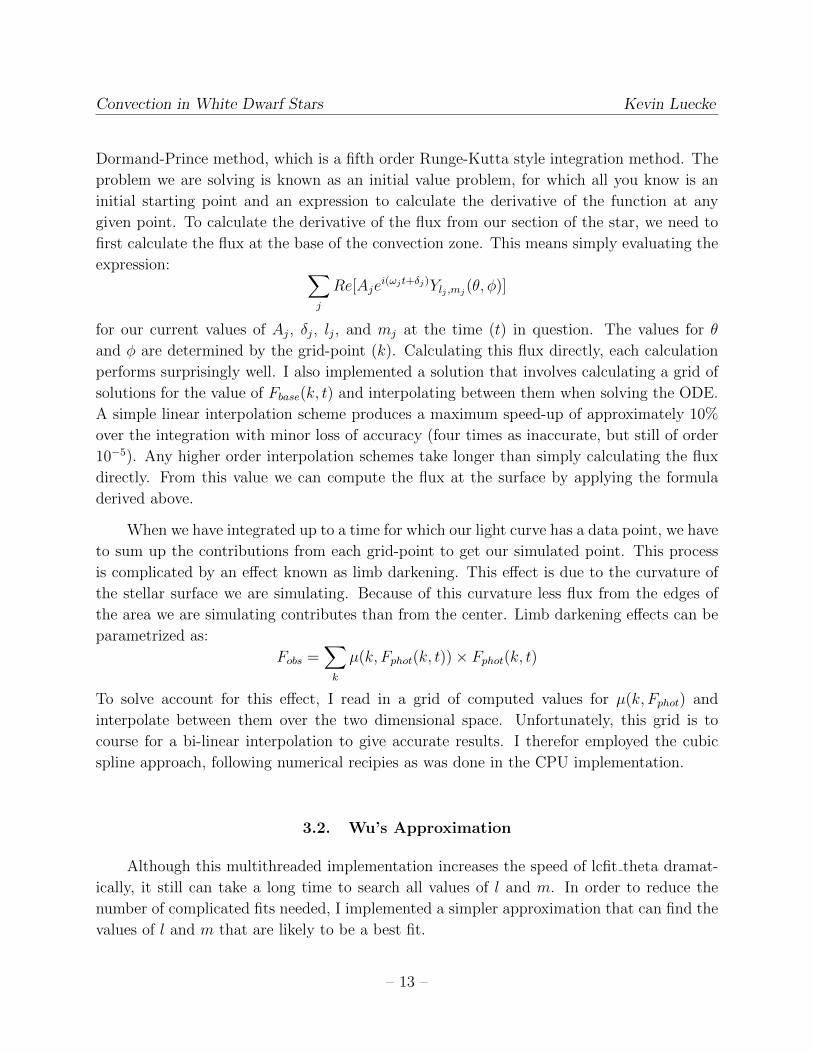
3.2. Wu’s Approximation
Although this multithreaded implementation increases the speed of lcfit theta dramat-
ically, it still can take a long time to search all values of l and m. In order to reduce the
number of complicated fits needed, I implemented a simpler approximation that can find the
values of l and m that are likely to be a best fit.
– 13 –
Convection in White Dwarf Stars Kevin Luecke
I took this formulation from the work of Wu in 2001 (cite). This approximation takes
the same form as the model of the flux at the base of the convection zone:
F =∑j
Re[Ajei(ωjt+δj)Ylj ,mj
(θ, φ)]
It simply changes apparent amplitude (A) and phase (δ) of each witnessed mode to approx-
imate the effects of a convection zone of base size τ0 according to:
Aphot =Afbase√
1 + (ωfbaseτ0)2
δphot = δfbase − arctan(ωτ0)
To implement this, I still divide the surface into a grid, but for each point I simply
calculate the flux at each timestep according to the above equations. I have also implemented
this fitting method with GAMA, so it can take full advantage of all the the host computer’s
resources while it is running. As it does not require an integration, this technique runs orders
of magnitude faster than the full integration.
Wu’s method does not always find the same values as ’best fit’ as the full integration,
however, it does seem to find better fits for the same values of l and m. In order to test this,
I have run both methods on a few stars simple enough to preform an exhaustive search with
the full integration method. So far it Wu’s method has identified all of the same of the values
that the full integration has identified. While this does not prove that Wu’s method will
identify the “best fit” according to the Montgomery’s method, it does give us a technique
for intelligently narrowing the set of l and m values that we calculate fully.
4. Targets and Data Acquisition
In order to test this theory I have chosen a number of targets that have been fit by
the linear version of lcfit theta, to judge the accuracy and performance enhancements of
my implementation. Those targets include: PG1351, G-2938, GD154, EC14012, WDJ1524,
and GD358. On top of that, however I have chosen a target that will test its capabilities,
HS0507+0435.
4.1. HS0507
This target tests the limits of my program as it has many more oscillatory modes than
the aforementioned stars, as well as a few closely spaced modes that require a few nights of
– 14 –
Convection in White Dwarf Stars Kevin Luecke
data to resolve. This means it has a large set of parameters to fit, as well as a long time
period to integrate over on each fit.
This star was the subject of a recent paper by Fu et al. (who refer to the star as
HS0507+0434B). In this paper, Fu lists 18 independent frequencies as well as a number of
other signals due to the nonlinearities in the light curve. Fu includes a set of “preliminary
identification[s]” of the l and m values as well as a discussion of their constraints of these.
Using lcfit theta we can determine these values more reliably. Fu notes that in his runs
he found variation in the excited pulsation frequencies, and that “More observational data
and theoretical investigations are needed to explore the physical causes of those visibilities”.
Fu discussed data from runs starting in 2007 and 2009. I have worked with people at the
University of Texas, The Central Texas Astronomical Society, and [paul?] to reclaim 36-inch
telescope at McDonald Observatory to collect further data.
4.2. Instrumentation
I had a few problems setting up the 36-inch for science. We wanted to clone an ex-
periment that was running on the 82-inch telescope at McDonald Observatory. The system
started with a spare camera and acquisition computer from the 82-inch telescope. This equip-
ment had been used to develop the 82-inch system, so it should have been fully functional,
however, it hit a few snags on the 36 -inch. The first of these problems manifested itself as
an unusually high level of static on every image we took. By systematically switching out
components with their counterparts on the 82-inch telescope I was able to determine that
the problem was with the camera itself. The broken component turned out to be a small chip
that monitored temperature levels for the camera cooling system. Without this component,
the camera was not able to sense its own temperature, so it would not cool. The noise we
had seen was just thermal noise from the ambient room temperature. The mounting screws
used were a bit too long and had penetrated just far enough into the camera to hit this
component. Fortunately, this was a relatively inexpensive part, and we were able to order a
replacement.
The second problem we encountered manifested as a series of bands that appeared across
the image. This turned out to be a high frequency interference originating from the motor
that controlled the stepping of the telescope when tracking. The signal was passing along
the wire that transferred the analog image to the control box. As the frequency was high
we had to ground the control box to the telescope, by mounting it on the telescope directly.
Later that year, Argos, the camera used for out parent experiment on the 82-inch
– 15 –
Convection in White Dwarf Stars Kevin Luecke
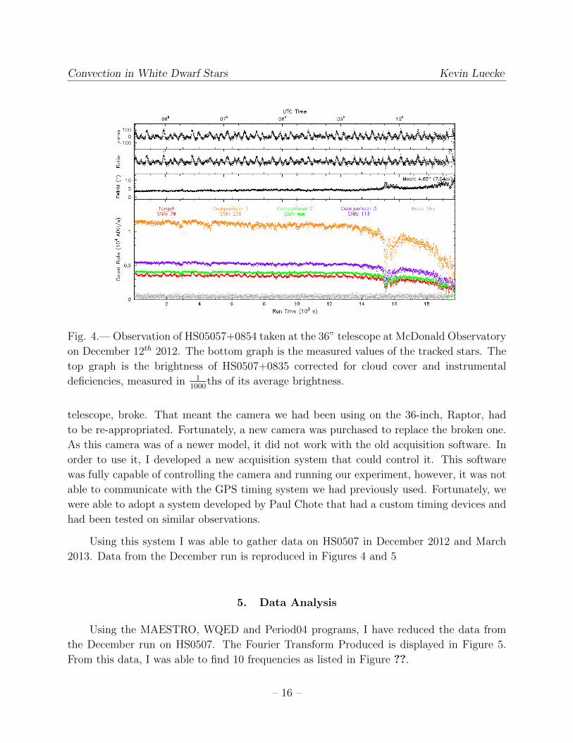
Fig. 4.— Observation of HS05057+0854 taken at the 36” telescope at McDonald Observatory
on December 12th 2012. The bottom graph is the measured values of the tracked stars. The
top graph is the brightness of HS0507+0835 corrected for cloud cover and instrumental
deficiencies, measured in 11000
ths of its average brightness.
telescope, broke. That meant the camera we had been using on the 36-inch, Raptor, had
to be re-appropriated. Fortunately, a new camera was purchased to replace the broken one.
As this camera was of a newer model, it did not work with the old acquisition software. In
order to use it, I developed a new acquisition system that could control it. This software
was fully capable of controlling the camera and running our experiment, however, it was not
able to communicate with the GPS timing system we had previously used. Fortunately, we
were able to adopt a system developed by Paul Chote that had a custom timing devices and
had been tested on similar observations.
Using this system I was able to gather data on HS0507 in December 2012 and March
2013. Data from the December run is reproduced in Figures 4 and 5
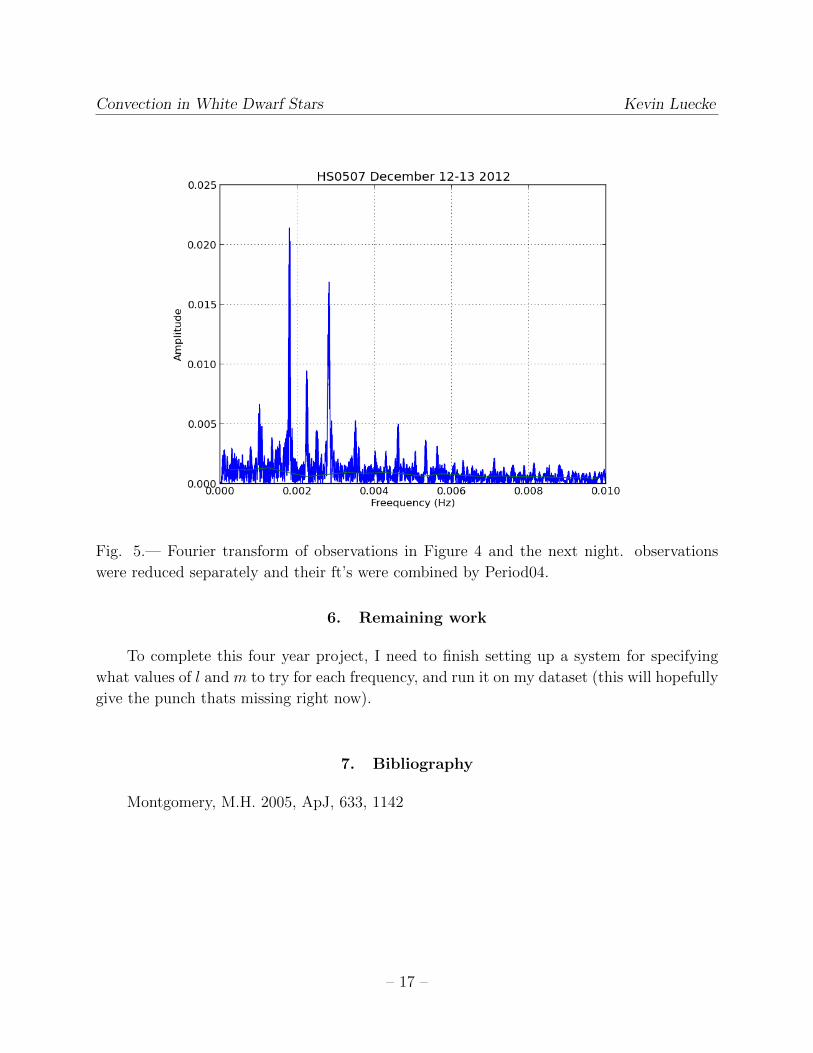
5. Data Analysis
Using the MAESTRO, WQED and Period04 programs, I have reduced the data from
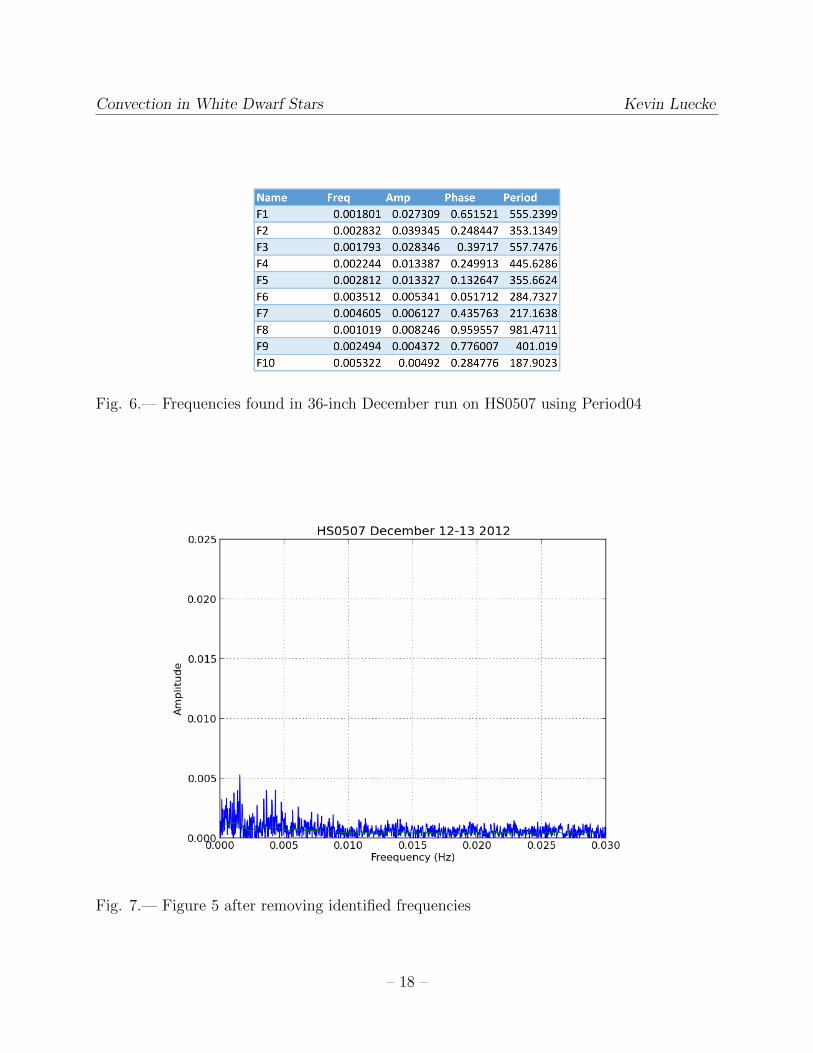
the December run on HS0507. The Fourier Transform Produced is displayed in Figure 5.
From this data, I was able to find 10 frequencies as listed in Figure ??.
– 16 –
Convection in White Dwarf Stars Kevin Luecke
Fig. 5.— Fourier transform of observations in Figure 4 and the next night. observations
were reduced separately and their ft’s were combined by Period04.
6. Remaining work
To complete this four year project, I need to finish setting up a system for specifying
what values of l and m to try for each frequency, and run it on my dataset (this will hopefully
give the punch thats missing right now).
7. Bibliography
Montgomery, M.H. 2005, ApJ, 633, 1142
– 17 –
Convection in White Dwarf Stars Kevin Luecke
Fig. 6.— Frequencies found in 36-inch December run on HS0507 using Period04
Fig. 7.— Figure 5 after removing identified frequencies
– 18 –