(BASA-TP-2469) CCNVERGENCL OF b Z ' I T O N v S i!Wi"i'OD FOS I S I b G l E 6 k A L I G U I T I C N ( N A S A ) 23 p BC k 0 2 / n F A0 1 CSCL 128

, b

L . c . l.e j - . f ' # ! - . A,: . . ,

-. - . . .* \ .

. . 4 i .

Unclas H I / b 4 20843

. . I NBA

/ : , t~chnical , . .

i P-r, . '

. 2$89 ' .j

: h . 1 9 8 5 4 1, , 3 % .i . . * -

, 4 , '

, . ..

Convergence of Newton's Method for a ' Single Real Equation

,.

(. -

C. Warren Campbell

https://ntrs.nasa.gov/search.jsp?R=19850020344 2018-04-17T05:03:44+00:00Z

. . I . . % .

, + , k p , , .: % . ~ T i k ~ 9

NASA Technical Paper 2489

Scientific and T e ~ h , i ~ c & I Information Branch

Convergence of Newton's Method for a Single Real Equation

C. Warren Campbell

George C. Marshall Space Flight Center Marshall Space Flight Center, Alabama

TABLE OF CONTENTS

INTRODUCTION . . . . . . . . . . . . . . . . . . . . . . . . . . . . . . . . . . . . . . . . . . . . . . . . . . . . . . . . . . . . . . . .

. . . . . . . . . . . . . . . . . . . . . . . . . . . . . . . . . . . . . . . . . . . . ASSOCIATED FUNCTION EXAMPLES

CONVERGENCE INSlDF. PRIMARY CONJUGATE POINTS . . . . . . . . . . . . . . . . . . . . . . . . . . . . .

. . . . . . . . . . . . . . . . . . . . . . . . . . . . . . . . . . . . . . . . . . . . . . . . . . . . . . . . . . . Assunlptions . . . . . . . . . . . . . . . . . . . . . . . . . . . . . . . . . . . . . . . . . . . . . . . . . . . . . . . . . . . . Conclusion

. . . . . . . . . . . . . . . . . . . . . . . . . . . . . . . . . . . . . . . . . . . . . . . . N POINT ITERATION CYCLES..

. . . . . . . . . . . . . . . . . . . . . . . . . . . . . . . . . . . . . . . . . . . . . . . . . . . . . . . . . . . . . . . . . REFERENCES

Page

LlST OF ILLUSTRATIONS

Figure Title I'age

1. Newton's iteratioll. . . . . . . . . . . . . . . . . . . . . . . . . . . . . . . . . . . . . . . . . . . . . . . . . . . . . . . 1

1 -. Iteration between primary conjugate points for f (x) =. cos(x) . . . . . . . . . . . . . . . . . . . . . . 3

3. Iteration between conjugate points for f(x) = cos(x). . . . . . . . . . . . . . . . . . . . . . . . . . . . . 3

4. f(x) 2nd associated function for f(x) = cos(x) + c, c = O., 0.25, and 0.5. . . . . . . . . . . . . . . 6

>. Function and associated function for f ( s ) = cos(x) + c , c = 0.75, 1.0. and 1.1 . . . . . . . . . 7

6. Function and associated function for f(x) = arctan(x) + c, c = O., 1 . . . . . . . . . . . . . . . . . 8

7. Function and associated !'unction for f(x) = x- + c, c = -1 .. O., 0.1 . . . . . . . . . . . . . . . . . . 9

8. 3 Function and associated function for f (x) = x - x - c , c = -3'13, 0 . . . . . . . . . . . . . . . . . 11

9. 2 Funct!on and associsted function for f(x) = ( -39118)~ + (67/72)x- + ? 17 5 7

- 1 + (1124)s ' + c , c = O . . I . . . . . . . . . . . . . . . . . . . . . . . . . . . . . . . . . . . . . . . . . 13

10. Function and associated function for f (x) = tan(x! + c. c = 0.. 1 . . . . . . . . . . . . . . . . . . . . ! 4

1 1 . Function and associated function for f (x) = arcsin(x). . . . . . . . . . . . . . . . . . . . . . . . . . . . IS

LIST OF TABLES

Table Title Psge

1. Some Corijugate Points for f (x) = cos (x) . . . . . . . . . . . . . . . . . . . . . . . . , . . . . . . . . . . . . 4

1 -. C'onjugdte Points arid It2rations for fix) = arctan(x) . . . . . . . , . . . . . . . . . . . . . . . . . . . . . 5

3. A Three Point Cycle for f (x) = cos(x> . . , . . . . . . . . . . . . . . . . . . . . . . . . . . . . . . . . . . . . 16

NOMENCLATURE

A(x) = associated function = Ax + Axl

An(x) = n-point associated function = Ax + A x , + . . . + Axn-,

f(x) = function whose zeroes are t o be f ,und

g(x) = Newton iteration function = x - f(x)/fl(x)

1 = g(x), an alternate notation

x ,x * = primary conjugzte points, x P P P < X ~ *

Xz = x-axis location of a zero of f(x)

Axi = ith Ax = -f(xi)/fl(xi)

NASA TECHNICAL PAPER

CONVERGENCE OF NEWTON'S METHOD FOR A SINGLE REAL EQUATION

INTRODUCTION

Newton's method is a well known technique for finding the zeroes of a nonlinear equation. For simple functions which can be differentiated, it can be easily programmed on a programmable calculator. This ease of programming permits an approach which is termed "experimental mathematics" in this paper. Experimental mathematics refers to the use of a computer with a user friendly graphics package. Much can be learned about extremely complex functions which are intractable using normal analytical methods. Using intuition, and experimental mathematics, a convergence conjecture for Newton's method was formulated. This conjecture is based on finding the zeroes of an associated function which is defined below.

Newton's method has the following convenient geometric interpretation. Starting with initial guess x, calculate the slope of f at x, draw the line through f(x), with slope fl(x), and extend the line to the x-axis. Where the line hits the axis is the next iterate (Fig. 1). Now consider a specific example, f(x) = cos(x). For this periodic function, one zero is as good as another, so attention is focused on the zero at x, = pi/2. Near this zero, Newton's method clearly converges. As the initial guess moves away from the

zero, convergence becomes less certain. Convergence of single point iteration functions is frequently investigated using the Contraction Mapping Theorem [ 1 I . The theorem is stated as follows.

Contraction Mapping Theorem [ 1 I : Let g be a continuous iteration function mapping a real closed interval, I into itself. Assume a positive constant L < 1 exists such that If(a) - f(b)l < Lla-bl for all a,b in I. Then in I there is a unique solution of the equation x = g(x) for any initial x in I.

Figure 1. Newton's iteration.

The Contraction Mapping Theorem provides sufficient, but not necessary conditions for con- vergence of the iteration function g(x). The conservative nature of the theorem will be demonstrated below.

Consider again f(x) = cos(x). Let an initial guess near the zero xz = pi12 move gradually away

from the zero. For a t:.ne as the initial guess moves away from xZ, Newton's method converges.

Intuitively, a point can be reached where the first iterate is on the opposite side of xz from the initial

guess and the second iterate is back at the first point. Without cornputational errors, then Newton's method would oscillaie back and forth between the two points forever. When two such points exist for a given func- tion, they will be called conjugate points and are said to be conjugate to each other. This terminology should not be confused with conjugates of the complex n~mbers. Intuitively, Newton's method might be expected - to converge inside the conjugate points. The purpose of this paper is to demonstrate that under certain con- ditions, Newton's met!!od will converge within these conjugate points.

The concept of conjugate points can be made more concrete with some analysis. Newton's d iteration is given by the following equation.

The second iterate is given in terms of the first in the same fashion.

If x2 = x is set, the following equation must be satisfied.

A(x) is called the associated function in the remainder of this paper. By inspection, fixed points of g(x) are also solutions of A(x) = 0. For f(x) = cos(x), g(x) = x + cot(x), and A(x) = cot(x)+ cot((x)+ cot(x)). From the definition in equation (3), A(x) goes to ioo if fl(x) or fl(x go to zero (as long as f does not go to

zero at x or x l ) If a function f has a zero at x,, and has a set of conjugate points, x and xp*, such P that x < xz < xp*, wit6 no other conjugate points falling in the interval (xp,xp*), then x and xp* P P' are called primary conjugate points. For f(x) = cos(x), a set of primary conjugate points exist around each zero. Figure 2 depicts Newton's iteration between the primary conjugate points around xz = pi/2.

Intuitively, moving toward the origin from xp other conjugate points should exist corresponding to

points on different waves of the periodic function cos(x). This is indeed the case, and f(x) = cos(x) has a countably infinite number of conjugate points on (O,pi/2). No pair of these points is conjugate to each other but are conjugate to points on the other side of x = pi/2. The first three conjugate points of f(x) = cos(x) are depicted in Figure 3.

'

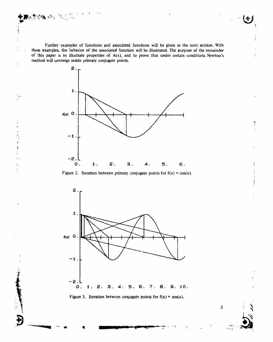
Further examples of functions and associated functions will be given in the next section. With these examples, the behavior of the associated function will be illustrated. The purpose of the remainder of this paper is to illustrate properties of A(x), and to prove that under certain conditions Newton's method will converge inside primary conjugate points.

Figure 2. Iteration between primary conjugate points for f(x) = cos(x).

Figure 3. Iteration betwcen conjugate points for f(x) = cos(x).

ASSOCIATED FUNCTION EXAMPLES

L

In the previous section, the Contraction Mapping Theorem was given, and described as overly conservative. Consider now the case for f(x) = cos(x), with corresponding iteration function g(x) = x +

I cot(x). For the theorem to app!y, g must satisfy a Lipschitz condition which may be restated as /gl(x) I < 1 on the convergence interval. For the fixed point at xZ = pi/2, the corresponding interval is

(pi/4,3pi/4) which is approximately (0.7854, 2.3562). In actual fact the convergence interval is more like (0.4052, 2.736). Obviously, the Contraction Mapping Theorem is quite conservative.

The actual convergence interval for f(x) = cos (x), is given by approximate values of the primary conjugate points asso~iated with the zero at pi/2. In the previous section, three sets of conjugate points were given graphically. Table I gives numerical values t o several decimal places. These conjugate points were calculated using an HP 11C programmable calculator, and they may not be accurate in the last one or two decimal places given. In fact, for f(x) = cos (x) the zeroes of the associated function were found using Newton's method. For other more complicated functions, differentiation of A(x) is difficult, and solution by the secant method [2] was convenient.

TABLE 1. SOME CONJUGATE POINTS FOR f(x) = cos(x)

While in principle, Newton's method will iterate for all time between the pairs of conjugate points given above, in practice the iteration begins t o wander away from the points because of roundoff and function evaluation errors. For the primary conjugate points, on the author's HP I IC, the iteration wanders away only in the last decimal piace on the first iteration for the primary conjugate points. For succeeding iterations, the divergence continues. Intuitively, from the geometrical interpretation of Newton's method, one might expect that the farther the distance between the two conjugate points, the faster the divergence. This is indeed the case. If one takes the values for the primary conjugate paint xp

and adds 1 in the last decimal place to put an initial guess infinitesimally inside the convergence interval, the iteration will begin to converge. If on the other hand, 1 is subtracted from xp, in the last decimal place, the iteration begins to diverge.

Location of the conjugate points of cos(x) is a hit or miss propositi?~, (mostly miss) and the higher order conjugate points are hard to find because of the discontinuous nature of A(x). A(x) can be studied quite easily, however, with a set of good computer graphics routines. If f(x) can be differentiated,

f

i A(x) can be plotted. The graphical exploration of the complex composite function A(x) falls in the realm of experimental mathematics and this section is devoted to this exploration for several examples.

The periodic function cos(x) is generalized by adding a constant so that f(x) = cos(x) + c. Figures 4 and 5 are plots of f and A for different values of c. For xp = 0.405 . . . observe that A(x) crosses the

x axis with positive slope. The slope of A(x) can be calculated in general.

From equation (4), if f' does not go to 0 at s zero of f, then at the zero the slope of A is -1. If A is continuous on (x ,x *), then it is positive on (xp,xZ), and negative on (xz,xp*). For every zero of P P f(x) = cos(x), this situation applies. As one looks at examples, this behavior will be observed frequently.

Figures 4 and 5 show that as long as c lies between 0, and 1, A(x) varies rather smoothly with c. As soon as c goes to 1 and then to greater values, the character of A(x) changes abruptly and radically. Since F(x) = cos(x) + 1.001 has no zeroes, the sudden change is not unexpected. Observe that just

.: because a function has no zeroes, the function may still have co~jugate points as is the case for cos(x) + c where c is greater than 1.

One of the purest examples possible of primary conjugate points and Newton's method converg- 6' ence is given by f(x) = arctan(x). For this case, both f(x) and A(x) are continuous on the infinite interval, e f(x) has one zero, and A(x) has three zeroes corresponding to two primary conjugate points and one zero ,- . at the origin. Figure 6 depicts these functions. Table 2 gives ilumericel values for the conjugate points of

arctan(x), and the first few iterations for different guesses.

TABLE 2. CONJUGATE POINTS AND ITERATIONS FOR f(x) = arctan(x)

Iteration

1

2 3

4

5

6

7

The iterations given in Table 2 are a dramatic demonstration that Newton's method converges inside primary conjugate points. Althougl~ primary conjugate points exist for many functions, some functions do not have conjugate points, and the only solutions to A(x) = 0 are those for which f(x) = 0.

2 The next example presented is f(x) = x + c which is shown in Figure 7. For c = -1, f has ziroes at *1. This is an example of function which is concave upward (f"(x) greater than 0) on the infinite interval. Functions which do not change curvature at least mice cannot have primary conjugate points. For the caw c = -1, the only discontinuity in A(x) occurs at f'(x) = 0, i.e., at x = 0. Because of the

0. 1. 2. 3. 4. 6. 6.

Figure 4. f(x) and associated function for f(x) = cos(x) + c, c = O., 0.25, and 0.5.

Figure 5. Function and associated function for f(x) = cor(x) + c, c = 0.75, 1 .O, and 1 . 1 .

I

3. 4l f (x) = arctan i x + 1.0 i

Figure 6 . Function and associated function for f(x) = arctan(x) + c, c = 0. 1 .

2 Figure 7. Function and associated function for f(x) = x + c, c = -I., O., 0.1.

concavity of the function and its position relative to the x axis, no Newton iterate x l can be equal to

zero. The spikes in A(x) normally associated with f r (x l ) = 0 do not occur for this case. The slope of A(x) at the two zeroes is -1 as before.

For the case when c = 0 , the form of A(x) changes drastically. The spike disappears and A(x) becomes a straight line through the origin with slope -314. This is the case where both f and f' go to

zero at xZ. Consider the general case of f = xn. In this situation, A(x) is always a straight line through

the origin with the following slope.

Notice that if n = 112 corresponding to f(x) = x1I2, A(x) = 0 for all x. In fact, if x is defined

as (-x)lt2 for negative x, and x1I2 for positive x, it is found that every point is a conjugate point! This remarkable fact can be approached from another direction. Consider an odd function, i.e., f(x) = -f(-x). For every point t o be a conjugate point, -x = x - f(xj/ft(x). Solving this little differential equation

gives f = kx112.

2 For the case, f(x) = x + 0.1, the character of A(x) again changes. When c was negative, A had one spike at the origin. When c was 0, A was a well behaved straight line. For c positix, A has three spikes. These three spikes correspond to the one place where fl(x) = 0, and the two places where f r (x l ) =

0. Notice that there are two conjugate points on either side of the origin, but they are not primary con- jugate points because there is no zero in between.

The next example. depicted in Figure 8, is f(x) = x j - x + c. For c = 0, this function has three zeroes at -1, 0, and + l . The function also has a point of inflection at the origin. A point of inflection is a necessary condition for the existence of primary conjugate points and the zero at x, = 0, has two

primary conjugate points. Again, it is seen that the spikey nature of A(x) corresponds to ff(x), and

f1(xl) = 0. The slope of f goes to zero at t3-lIZ. For c = 0, Newton's method converges to the zeroes at .tl for guesses outside the zeroes of f'(r).

So far the fact that conjugate points can be overlapped has not been emphasized, i.e., xcl < xc2

<xCl*<xc2*. In fact. the construction of a function with conjugate points aL any location, with any

order of the conjugate points is possible. Geometrically, locations are chosen where conjugate points are desircd and the necessary line is drawn in with the correct slope that intersects the x axis at the desired location of the corresponding conjugate point. Do this for each set of desired conjugate points, and then draw in a curve through the desired values at the conjugate points and tangent at these points to the previously drawn lines and the result is a function with the desired properties. Mathematically, one can

d o the same thing with a polynomial function. For example, consider the odd function f = c l x + c2x3 + c3x5 + c4x7. This function should satisfy f(-2) = 2, f(-1) = I , f(0) = 0, f(1) = -1, and f(2) = -2. In

addition, corresponding conjugate points are needed at -2 and 1, and at -1 and 2. The required values of ci can be found and the result is given below.

Figure

-2. -1. 0. 1. 2.

8. Function and associated function for fix) = x3 - x - c, c = -3lI2, 0.

This fur~ction is plotted in Figure 9. One purpose of this exercise was to see if a function can have overlapping conjugate points without generating primary conjugate points inside the innermost con- structed conjugate points. For this example, a set of primary conjugate points were generated inside (-1 ,I). These occurred at xp = -0.7 1881058427 and xp* = 0.7 1881058427. This result raises the qties-

tion of whether it is possible to have a well behaved associated function without primary conjqate points but having overlapping nonprimary conjugate points. In this simple example, the hypothesized situation did not materialize. This point is still under investigation because, if possible, it limits the usefulness of the convergence theorem to be proved in the next section.

Usually, the composite associated function is more complex than f(x). For f(x) = tan(x) .t c, the opposite is true. The plot for this case is shown in Figure 10. For the tangent function, fixed points accur at 0, fpi/2, +pi, ... The fixed point at x = 0 is a legitirllate zero of tar,(x), but the futed point a1 pi12 corresponds to tan(x) = -. Because f'(pil2) = -, Ax goes to zero. For any initial guess, other than where the tangent is +, Newton's iteration converges to the nearest zero of the function.

Figure 11 corresponds to f(x) = arcsin(x). The associated function seems to have the desirable fonn with three zeroes, expected of primary conjugate points and a zero. This is not the case because the two outside solutions correspond to fixed points of Newton iteration and, hence. are not conjugate points.

In this section, the wonderfully varied nature of the associated function A(x) was investigated. The examples make plausible the hypothesis that when primary conjugate points exist around the zero of a function, then Newton iteration converges for initial guesses between xp and x *. Under certain conditions, this conjecture is proved in the next section.

P

CONVERGENCE INSIDE PRIMARY CONJUGATE POINTS

The proof of the conjecture that Newton's method converges inside pr;,mary conjugate points will be outlined before the actual proof so that some understanding of the approach is possible. The hypotheses of the Theorem are chosen so that the "standard" form of A(x) is assured. This form is A(xp) = A(x,) = A(xp*) = 0, and A(x) negative on (xp.xZ), and positive on (xZ,xp*) Once this is

achieved, then the only stumbling block is that the iteration once inside the conjectured convergence interval may wander back outside. For the "standard" form of A(x), this is shown to be impossible by contradiction. Then, because an initial guess on either side of the zero and in the interval will two iterations later be closer to the zero because of the positive and negative nature of A(x), then convergence is assured. The theorem follows.

Assumptions

1. ffx) and f(xl) are continuous, and have continuous first and second derivatives on an interval

[a,b]. f(x) has a zero at xz and corresponding primary conjugate poipts at x and xp* lying inside the interval [a,b] . P

2. f(xp)fl'(xp), f(xp*)fU(xp*), and fW(xp)f "(xp*) < 0.

3. fl(x), and f1(x1) f 0 on [xp,xp*].

Fidure 9. Function and associated function for f(x) = (-39118)~ + (67/72)x3 + (-13!36)x5 + (1/24)x7 + c, c = 0.,1.

1 ,. &p,\y,-??t&:3t~*. .. 2 c.. L 4- , .~ L d . - ~ * .

Figure 10. Function and associated function for f(x) = tiUl(x) + c, c = om, 1.

Figure 1 1. Function and associated function for f(x) = arcsin(x).

Conclusion

Newton iteration converges to x, for initial guess x in (x x *). P' P

From the hypotheses, g(x) is continuous on (x x *), and A(x) = 0 only at the two conjugate P' P

points and at the zero. At the zero, A1(x,) = -1. Then A(x) is positive on (xp,xz), and negative on

(x,,xp*). The proof f~ l lows quickly, if no point XT in I = (x x *) exists such that g(xT) > x * or P' P P

< xp. Consider the first case. Since g(xT) > x *, and since g is continuous, then there exists a point P

xa on (xT,xz) such that g(xa) = x *. Then A(xa) = xp - xa < 0. This cannot be since it has already been P shown that A is positivc in the interval to the left of x,. In order to have XT exist, another conjugate

point is required which violates the hypotl-esis of primary conjugate points. Now for x on I and less than x,, x < x2 < x4 < ... < ~2~ where x, ..., xzn-2 are in Il = (xp,xz), and xzn is in 12 = (x x *). Thcn,

Z' P because A is negative to the right of xz, xzn > xzn+2 > ... > x2i where the iterates from x2, to x2i-2

are all in 12- x2i falls in l l . This process is continued indefinitely, each time falling closer and closer to

x,, so that convergence to x, is clear.

This..concludes the proof. The hypotheses are stringent and may be overly restrictive. From the examples of the previoils section, m a y simple functions satisfy the hypotheses.

'i

N POINT ITERATION CYCLES

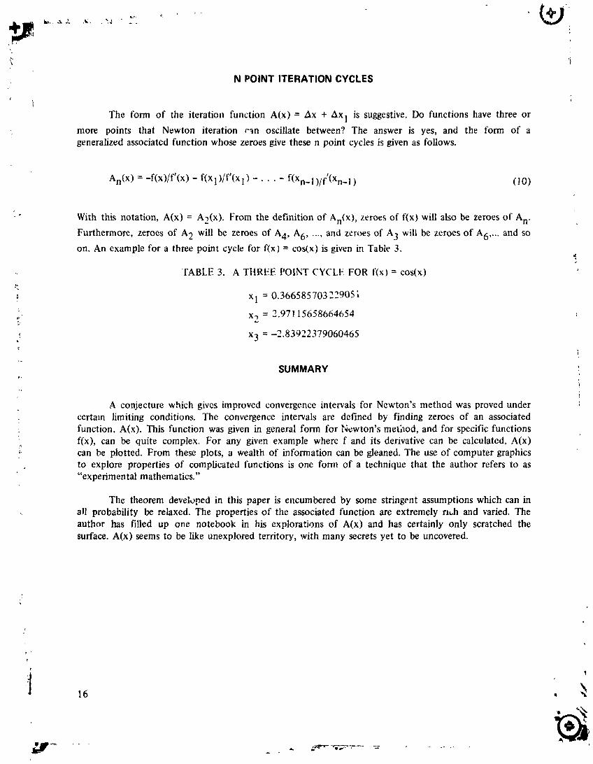
The form of the iteration function A(x) = Ax + Axl is suggestive. Do functions have three or

more points that Newton iteration r l n oscillate between? The answer is yes, and the form of a generalized associated function whose zeroes give these n point cycles is given as follows.

With this notation, A(x) = A?(x). From the definition of A,,(x), zeroes of f(x) will also be zeroes of An.

Furthermore. zeroes of A2 will be zeroes of A4, A6, ..., and zeroes of A3 will be zeroes of A6, ... and so

on. An example for a three point cycle for f(x) = cos(x) is given in Table 3.

TABLE 3. A THREE POINT CYCLE FOR f(x) = cos(x)

SUMMARY

A conjecture which gives improved convergence intervals for Newton's method was proved under certaln limiting conditions. The convergence intervals are defined by finding zeroes of an associated function. A(x). This function was given in general form for Piewton's method, and for specific functions f(x), can be quite complex. For any given example where f and its derivative can be calculated, A(x) can be plotted. From these plots, a wealth of information can be gleaned. The use of computer graphics to explore properties of complicated functions is one form of a technique that the author refers to as "experimental mathematics."

The theorem develeped in this paper is encumbered by some stringent assumptions which can in all probability be relaxed. The properties of the associated function are extremely n ~ h and varied. The author has filled up one notebook in his explorations of A(x) and has certainly only scratched the surface. A(x) seems to be like unexplored territory, l ~ i t h many secrets yet to be uncovered.

.! \ REFERENCES

. '

. 1. Wait, R.: The Numerical Solution of Algebraic Equations. John Wiley and Sons, New York, 1979.

i ' 2. Conte, S. D., and de Boor, Carl: Elementary Numerical Analysis: An Algorithmic P.pproach. McGraw-Hill Book Company, New York, 1972.

I ~, ,

>

. 1. REPORT NO. 2. GOVERNWNT ACCESSION NO.

TP- 2489 4. T ITLE AND SUBTITLE

Convergence of Newton's Method for a Single Real Equation

7. AUTHOR(S)

C. Warren Campbell 9. PERFORMING ORGANIZATION NAME AND ADDRESS

George C. Marshall Space Flight Center Marshall Space Flight Center, Alabama 358 12

A

12. SPONSORING AGENCY NAME AN0 ADDRESS

National Aeronautics and Space Administration Washington, D.C. 20546

15. SUPPLEMENTARY NOTES

. 3. RECIPIENT'S CATALOG NO.

5 . REPORT DATE June 1985

r

6. PERFORMING ORGANIZATION CClOE

0. PERFORMING ORGANIZATION REPOR r c

go. WORK UNIT NO.

M-49 1 11. CONTRACT OR GRANT NO.

13. TYPE OF REPORi & PERIOD COVERED

Technical Paper

14. SPONSORING AGENCY CODE

Prepared by Systems Dynamics Laboratory, Science and Engineering Directorate.

16. ABSTRACT

Newton's method for finding the zeroes of a single real function is investigated in some detail. Convergence is generally checked using the Contraction Mapping Theorem which yields sufficient but not necessary conditions for convergence of the general single point iteration method. The resulting convergence intervals are frequently considerably smaller than actual convergence zones. For a specific single point iteration method, such as Newton's method, better estimates of regions of convergence should be possible. A technique is described which, under certain conditions (frequently satisfied by well behaved functions) gives much larger zones where convergence is guaranteed.

17. KEY WORDS

Numerical Analysis Newton-Raphson Method Iteration

18. DISTRIBUTION STATEMENT

Unclassified-Unlimited

STAR Category: 64

22. PRICE

A0 2

19. SECURITY CLASSIF. (d t b b -DM)

Unclassified

-20. SECURITY CLASS1 F. (of tNm pee)

Unclassified

21. NO. OF PAGES

2 1