AD-A228 407

Naval Ocean Research andDavelopment Activity NORDA Technical Note 427Stennis Space Center, Mississippi 39529-5004 September 1990

Converting Digital Passive MicrowaveRadiances to Kelvin Units

of Brightness Temperatures

L. D. FarmerD. T. Eppler

A. W. LohanickOceanography Division

Ocean Science Directorate

nFjFP;IODUGED fYU.5. DEPARTMENT OF COMMERCE

NATIONAL TECHNICALIfrrOnMATION ar RVICEsPnItjoFIELD, VA 22161

Approved for public release; dltrIbutlon IS unlimhed. Navai Ocean Resre- lth and Deveiopment Activity, Sis spaceCenter, M199l99lpp1 39529-5004.

90 1

DISL ADENOTICE

THIS DOCUMENT IS BES..TQUALITY AVAILABLE H COPY

FURISEDTO DTC CONTAINEDA SIGNIFICANT NUMER OFPAGES WHIC DO NOTREPRODUC -LGILY.

ABSTRACT

The Ka-band Radiometric Mapping System (KRMS) has been utilized since 1983 to collectdigital records of microwave radiances. This report details methods for converting thesedigital radiances to appropriate units of brightness temperature.

L

I,€

-7

ACKNOWLEDGMENTS

The work reported here was supported by NOARL (formerly NORDA) Program Element61153N (Herbert Eppert, Program Manager), and by the NASA Oceanic Processes Branchthrough the SSM/I Validation Program (Robert Thomas, Program Manager).

ii

. ..k. . . . .. ... .. . ..

CONTENTSPage'

Abstract....................................................................................Acknowledgments.....................;......................................... I.............. iiIntroduction ................................................................................Background.................................................................................. 2Conversion methods .......................................................................... 3Digitizing ...................................................................................Conclusions.................................................................................. 5References ................................................................................... 6Appendix A: Brightness temperature conversion charts .................................. 7Appendix B: Distribution list................................................................ 13

ILLUSTRATIONS

Figure1. Reference load voltage to temperature conversion chart..........................I2. Determining proper reference load voltage...........................................-

TABLE

Table1. Comparison of sensor temperature with ambient and adjust ambient tempera-

ture for KRMS missions flows between 1984 and 1988 ....................... 4

, -

Converting Digital Passive Microwave Radiancesto Kelvin Units of Brightness Temperatures

L. DENNIS FARMER. DUANE T. EPPLER AND ALAN W. LOHANICK

INTRODUCTION

NOARL, in conjunction with the Naval Weapons Center (NWC) at China Lake, Califor-nia, has been collecting passive microwave imagery with the K -band Radiometric MappingSystem (KRMS) since 1983. With the exception of the 1983 data, none of these data havebeen converted to brightness temperatures. The KRMS is not a calibrated system; however,the 1983 data were converted to brightness temperatures using the engineering method de-scribed in NORDA Report 51 (Eppler et al. 1984), which required measuring the gains andlosses within the system and then scaling the resultant radiances to surface-measured valuesfor open water and first-year ice.

The system has a measured reference load that may be related to brightness temperature

using the conversion graph produced at NWC (Fig. 1 ). This provides a warm reference point.The cool reference point (or tie-point) used is an assumed brightness temperature for openwaterat nadir, 135 kelvins (K). Another possible method is to use a local ambient temperature

at the surface adjusted for the highest anticipated emissivity for sea ice (0.94) and use this asthe warm tie-point.

318

-313

38-303

E

298

_-28

-243

2 Figure 1. Reference load oltage to

233 temperature (K) conversion hart.

if6

I

B0

reference loadvoltage

,: B- 0 (scaled to 10 V/1O2ref voltage/, = reference load voltage for use with

conversion graph

Example A. B1 =9.5V A1 = (B1-B0)/10 = 0.95

B0 =0 A2 = ref/Al = -2.63Sensor temp - 260 kelvins

Reference load -2.5 V

B. B1 = 11.5VAl = 11.5-(-1.5)/10 = 1.3

B0 -- 1.5

Sensor temp 260 kelvins A2 = 5.0/1.3 = 3.85

Reference load 5.0 V

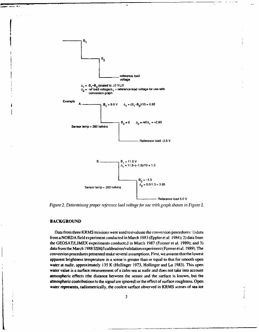
Figure 2. Determining proper reference load voltage for itse with graph shown in Figure 1.

BACKGROUND

Data from three KRMS missions were used to evaluate the conversion procedures: I ) datafrom a NORDA field experiment conducted in March 1983 (Eppler et al. 1984); 2) data fromthe GEOSAT/LIMEX experiments conductcd in March 1987 (Farmer et al. 1989); and 3)data from the March 1988 SSM/ calibration/validation experiment (Farmer et al. 1989). Theconversion procedures presented make several assumptions. First, we assume that the lowestapparent brightness temperature in a scene is greater than or equal to that for smooth openwater at nadir, approximately 135 K (Hollinger 1973, Hollinger and Lo 1983). This openwater value is a surface measurement of a calm sea at nadir and does not take into accountatmospheric effects (the distance between the sensor and the surface is known, but theatmospheric contributions to the signal are ignored) or the effect of surface roughness. Openwater represents, radiometrically, the coolest surface observed in KRMS scenes of sea ice

2

(Eppler et al. 1986). Since

Tb=E xT t (1)

where Tb is the brightness temperature, E the emissivity and Tt the physical temperature, wecan relate Tb to the physical temperature of a surface. If we assume that the emissivity of acalm sea is 0.50 at nadir, and that the thermal temperature of exposed arctic seawater is at itsfreezing point (-1.8* C or 271.36 K), then, from eq 1, the brightness temperature (Tb) of openwater measured at the sea surface is 136.68 K. Hollinger (1973, 1983) and Stogryn (1971)predict similar values. Second, we assume that the highest brightness temperature can beestimated using either a known surface temperature (ambient) or by measuring the referenceload voltage and computing the equivalent brightness temperature from the NWC graph (Fig.1 ). If these assumptions hold, then the range of digital radiance values present in a KRMS dataset can be linearly scaled to brightness temperatures that fall within this range. Our approachis to define tie-points that represent cool and warm radiances of known value. Response ofthe radiometer is assumed to be linear between these extremes, which allows brightnesstemperatures to be assigned to radiances that fall between these extremes by linear interpo-lation.

The engineering method presented in NORDA Report 51 used 139 K for open water and240 K for the high temperature, and applies only to the 1983 data set.

CONVERSION METHODS

The cool tie-point for both methods is represented by the radiometrically coolest surfaceobserved in scenes of sea ice, open water at nadir. For our purposes, we have used 135 K. Thewarm tie-point is determined by using either a local ambient temperature, adjusted for thehighest anticipated emissiity, or the reference load equivalent sensor temperature.

The first method discussed uses the ambient surface air temperature adjusted by theemissivity of first-year ice. Since eq I relates radiometric brightness temperature (Tb) in kelvinsof a body with emissivity (E) to its physical temperature (Tt) in kelvins, and E ranges from0.0 to 1.0, the radiometric temperature (Tb) of a substance should not exceed its physicaltemperature (T,). The emissivity of any natural surface is less than 1.0, so the highest an-ticipated radiometric temperature in a scene is necessarily less than its physical temperature.Since first-year sea ice and some forms of young ice have the highest emissivity (0.94) of theobjects scanned in these surveys, they will display the highest radiometric temperatures ob-served in KRMS images. We assume that the highest radiometric temperatures measured ina region correspond to areas of young first-year sea ice, and that the radiometric temperatureof these surfaces is about 0.94 times the local physical temperature, expressed in kelvins.

The second method uses an internal reference load and equivalent sensor brightnesstemperature for the warm tie-point. There are three voltages measured at test points on theoperator's console: B1, B0 , and the reference load. B I is the level of the highest radiometersignal, B0 is the level of the lowest radiometer signal, and the reference load is the voltagelevel to which the radiometer voltages are forcibly referenced. KRMS data are digitizedacross a 20-V range, with the highest signal level set at 10 V and the minimum at - 0 V. Thusthe B I value has to be scaled to 10 V by dividing (B 1-130) by 10, and then scaling the referenceload by dividing it by the result of (BI-B 0)/10. Figure I is a graph produced at NWC byplacing a thermocouple at the reference load and varying the reference load voltage and

3

Table 1. Comparison of sensor temperature withambient and adjusted ambient temperature for KRMSmissions flown between 1984 and 1988.

Adjusted.Senso'tr flltnp Ambtient temp (11nhientt Imttp

Dute (K) (K) (K)

I July 1984 2883 July 1984 27821 March 1987 288 274 25823 March 1987 27624 March 1987 280 272 25626 March 1987 276 255 24027 March 1987 273 25729 March 1987 273 25730 March 1987 273 2576 March 1988 273 257

274279

8 March 1988 280291 273 257280 248 233278276276

I I March 1988 279 276 2592802802,(0

280

280 267 25 1280

13 March 1988 279 259 243276276276 272 256276 272 256278279 259 243279 259 243

14 March 1988 275275275275275275278278278278278278276276 248 233

recording the resultant equivalent brightness temperature. Figure 2 illustrates the processused to obtain the reference load voltage used with the NWC graph to obtain the equivalentbrightness temperatures for this study. When analog data are digitized, the gain and offsetapplied to the analog signal are adjusted such that the reference load voltage corresponds toa digital value of 0. By deriving the brightness temperature that is equivalent to the referenceload and a digital value of 0. a warm tie-point is established. The cool tie-point, 135 K, is .setat adigital value of 2000, and the data scaled linearly between these tie-points. The equivalent

4

I

brightness temperature of the reference load has remained reasonably stable since 1984 andis always higher than the adjusted ambient temperature (Table I).

Figure A l provides both a comparison of the engineering conversion used for the 1983data and the corresponding conversion graph computed using a local adjusted ambient tem-perature and open water. In this instance, they compare favorably. Examples of brightnesstemperature conversions obtained using both methods are shown as Figures A I-Al7. Theaverage slope of the conversion equation for the ambient temperature/open water method is0.0584 with a standard deviation of 0.00549. The average slope for the sensor temperature/open water method is 0.0728 with a standard deviation of 0.0027. The difference is severalstandard deviations (see Fig. A 18). The ambient temperature method is greatly dependent onthe accuracy, locality, and the timeliness of the measurement. The sensor (reference loadequivalent) temperature has been very steady and is therefore recommended for use withexisting data.

DIGITIZING

When the analog data are digitized, the 0 digital value is normally set equal to the referenceload voltage. However, by observation, the lowest digital value corresponding to actual seaice is usually higher than 0. Thus, the actual digital value for the highest brightness tem-perature should be determined for each set of data being converted and this value used for thewarm tie-point.

CONCLUSIONS

Both methods evaluated produce brightness temperatures that appear to be reasonable forthe types of surfaces being imaged. The sensor temperature method produces values that areapproximately 20 K higher at the maxima; however, they compare reasonably well with ob-servations from other radiometers. The cool tie-point ( 135 K) for open water is questionableand is a source of error in both methods. The actuai*ital value for the warm tie-point isanother questionable point and will vary between data .

The ambient temperature method is predicated on the availability of timely and accuratesurface measurements of physical temperature and the validity of the assumption that thehighest brightness temperature in a scene is less than the measured ambient. This method isbased on surface datum and does not require that corrections be made for atmospheric con-tributions.

The sensor temperature method appears to be the more repeatable method. It producesbrightness temperatures that appear to be reasonable when compared with the March 1983data and other sources (such as surface-based measurements and airborne Advanced Multi-channel Microwave Radiometer data). This method is affected by the atmospheric con-tributions, as the warm tie-point is internal to the sensor. The cool tie-point (water) is a surfacemeasurement. Atmospheric models exist that may provide some value of correction for thebrightness temperatures derived using the sensor temperature and open water method. Thederived values presented in this report are few in number and are therefore insufficient to forma final conclusion as to the accuracy of this method and recommended for relative com-parisons only.

5

This investigation has not resulted in any method that consistently and reliably producescalibrated brightness temperatures and only serves to emphasize the need for the addition ofreal-time calibration sources to the KRMS sensor.

REFERENCES

Eppler, D.T., L.D. Farmer, A.W. Lohanick and M. Hoover (1984) Digital processing of

passive Ka-band microwave images for sea ice classification. Naval Ocean Research andDevelopment Activity, Stennis Space Center, Mississippi, NORDA Report 51.Eppler, D.T., L.D. Farmer, A.W. Lohanick and M. Hoover (1986) Classification of seaice types with single band (33.6-GHz) airborne passive microwave imagery. Journal of

Geophysical Research, 91(C9): 10,661-10,695.Farmer, L.D., D.T. Eppler, B. Heydlauffand D.A. Olsen (1989) KRMS GEOSAT/LIMEX87 Quick Look report. Naval Ocean Research and-Development Activity, Hanover, NewHampshire, NORDA Technical Note 385.Hollinger, J.P. (1973) Microwave properties of a calm sea. Naval Research Laboratory,Washington, D.C., NRL Report 7110-2.Hollinger, J.P. and R.C. Lo (1983) SSM/I project summary report. Naval Research Labo-ratory, Washington, D.C., NRL Memorandum Report 5055.Stogryn, A. (1971) Equations for calculating the dielectric constant of saline water. Instituteof Electrical and Electronics Engineers, Transactions on Microwave Theory and Techniques,MTT-19: 733-735.

6

APPENDIX A: BRIGHTNESS TEMPERATURE CONVERSION CHARTS

BMW=ON SEA MORDA Te Report SIAmbent Air I Open Water 125K *2047 V

240 ~~133K *2047DV 2020 SD

236K aODY (OW 4.061S) M 4 K

20 (DV * .0403) * 236 K 22K

Wis. Usin-

140 140-

13 * 1200 li 260 50 75'0 '10'00'12650 1500 1750 2000 0 250 500 7501001250'1500 17560 2000

DIGITAL VALUES DIGITAL VALUES

Figure Al. Brightness temperature conversion chart for March 1983.

MI

290.

too

,Sensor Tamp IOpeni Water

139 278K a OOY

to (DV - 4.0716) + 278 a K

lie 56@ SO 750 106 1250 16,00 176 200

DIWIAL VALUESFigure A2. Brightnes temspe rature conversion chart for3 July 1984.

V 7

2200

z m z-a m ,ml0

J LIMEX LIMEXSensor Temp / Open Water In0 Ambient Air I Open Water

i- 135K x 2000DV 135K a 20000V1 2$K a D 0V 260K a ODV

'-0 (DV - -0.0765) + 288 - K Jac (DV -0.0625) + 260 K100 . 1,0 - - -

0 250 500 750 1000 1260 1500 1750 2000 0 250 500 750 1000 1250 1500 1750 2000

DIGITAL VALUE DIGITAL VALUES

Figure A3. Brightness tenperature conversion chart for 21 March 1987.

300 200

260 240'

.j -1

S160 150.

I60 GREENLAND SEA 1IN GREENLAND SEASensor Temp / Open Water Ambient Air / Open Water

140. 135K = 2000DV 140 135K = 2000DV

1 D0.5276K 0 Dv 120 258K 0 DVm. (DV * -0.0705) + 276 x.K . (DV -0.0615) +258 = K

100 . 100"0 250 600 750 1000 1250 1500 1750 2000 0 250 500 750 1000 1250 1500 1750 2000

DIGITAL VALUES DIGITAL VALUES

Fi,,re A4. Brightness temperature conversion chart for Figu re A5. Brightness teniperatur' conzersio, chart for23 and 26 March 1987. 24 March 1987.

300 300

Me 240.

z m zILI~ -

in GREENLAND SEA 10TRANSIT FLIGHTAmbient Air / Open Water ISensor Temp / Open Water

10 135K * 2000DV iS125K a 2000DVIs 250K OY 274K a 0DV

(DV * -0.062) # 250 = K (V * -0.00) + 274 a K

e *is 506 l s 106$ 1sa 1is' 0 176 t2o 0oo 0 34000 740 160o 130 10o 1750 2600

DIGITAL VALUES DIGITAL VALUESFigu re A6. Brghtiess temrntne conversion chart fr Figure A7. Brightness t'niplkratunc conve'rsion chart fur27 and 29 March 1987. 6 March 1988.

200

zm

I" Cap. Llsburne,AKSensor Temp /Open Water

am- 278K O DV

1006 (DV * -0.0715) + 278 . K0* 250 500 760 10'00 12150 15!60 1750'20100

DIGITAL VALUESFigure AS. Brightness temperature conversion chart for8 March 1988, Cape Lisbu rne, Alaska.

300 300

200 200 KOTZEBUE, AKAmbient Air I Open Water

M- 280 135K u2000DV

236K u CV240- 240- (DV -0051) +236 +K

ISO0 KOTZEBUE,AKISSensor Temp / Open Water

140 135K =2000DV 140-

i20K =O 1D0(DV * -0.0725) + 280 a K10

106 1 1001a 250 100 750 '10'00'1250 1500 1750 20-00 i 250 S00 710 '100061250 1500 1750 200

DIGITAL VALUES DIGITAL VALUES

Figure A9. Brightness temperature conversion chart for 8 March 1988, Kotzebue, Alaska.

2K 200.

~~1w200-

160 NO

In. FAIRBANKS, AK log FAIRBANKS, AKAmbient Air / Open Water Sensor Temp / Open Water

14 35K =20000V 14 135K u20000V

(DV .065 *2OV 291 K -ODV(DVK *-.015 +211V (DV * -0.078) * 231 a K

e 266 850 750; e s e10 i 20 t ie se 6;@ 4 ieee9 11s Ise 176 Me0DIGITAL VALUES DIGITAL VALUES

Figure A10. Brightness temiperature conversion cha rt for 8 arch 1988, Fairbanks, Alaska.

9

31

-s

24 M.

5 M

.jJ

in FAIRBANKS,AK FIBNSACSensor Tamp / Open Water 10FA KAAmbient Air / Open Water14 3K a 2000DV 1 13K= OD279K w ODY 4' 3K-200

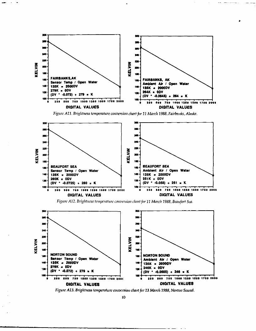
I (Dv* -0.072) + 279 a K 120. 264K a ODV_____0______00______ (DV ' -. 0645) +6 264 a K

0 25610go 710 1000 1;60 16500 17,50 20,00 o al 2;0 - s too0 - ? 40 11 00710 620

DIGITAL VALUES DIGITAL VALUESFigure All. Brightness temperature conversion chart fiw 11 March 1988, Fairbanks, Alaska.

z 2 20-

z 20

IS. BEAUFORT SEA In BEAUFORT SEASensor Temp / Open Water . Ambient Air / Open Water

140 135K -200ODV 140' 135K -2000DV

20 20K = DV '0251K = CV(DV - -. 0725) +280=zK (DV *-.058) +251 aK

* 20100 71 1000 121 1500?i l 17150 20'00 10 2 O50 60 716i 10'00 12160 1100 17'50 20

DIGITAL VALUES DIGITAL VALUESFigure A12. Brightness tempileratitre cot'ersion chart for 1 March 1988, Beaufort Sea.

20000g

5 . 2an

240 lo240

I10 N ORTON SOUND loo N ORTON SOUNDSnrTep / Open Water =mbient Air / Open Water

140 135K *2000DV 10135K a MODYIn 279K OD In,24KaVDI* (DV - -0.072) + 279 a K (DV 26K -0055 *O 2

0 210' 600' lie ll 00 110106170 0020 0 710'ie 1000 12 0 017,5012000

DIGITAL VALUES DIGITAL VALUESFigure A13. Brightness temperature conversion chart flr 13 March 1988, Norton Sounid.

10

z IM.

ST MATTHEWS ISLAND ~ ~ ST MATTHW ISANAmbientAir / Open Water Sensor Tamp I Open Water1 35K *2000DV 140- 135K u2000DV

264K =O 12ODY 0O(DV *4-.0645) + 264 a K (V*-.5 276 m 0K

0 250 500 750 10'00 12560 1500 1710 2000 a io '5;0 750* 1000'12'50 15009 1750 20'00

DIGITAL VALUES DIGITAL VALUES

Figure A14. Brightness temperature conversion chart for 13 March 1988, St. Matthews Island.

M. 20

20 200-

30 240-

Z 20 z 20 -> 200-

.j j

~19 ISO.

- BERING SEA CHUKCHI SEASensor Temp /Open Water SesrTm pnWater

I* r136K u 2000DV 140 135K a2000DV

In276K a0DV 10275K *ODY(DV * -. 0705) + 276 aK (DV * 4.070) + 275 z K

i. 2i i 1'0125 0 75'00 0 250 50 750 1000 1250 15'00 1750 2000

DIGITAL VALUES DIGITAL VALUESFig iireAl 5. Bri'ghtniess tern pieratu -e contz'ersiou chiart for Fiure Al6. Brighitness tern peratu reconiversion chiart for13 March 1988, Bering Sea. l4 March 1988, Chukchi Sea.

NO NO

M. BARROW, AK 3

Ambient Air / Open Water260135K =2000DV

a 233K =ODY 4(DV -04.049) +. 233 =K

umu

100 110BARROW, AKSensor Temp IOpen Water

1440' 135K -2000DV

20276K =0 DVS(DV ' -. 0705) + 276 z IK

* i ISO50 710 is00 1280 150W 1780 2003 5 7010 l 50 17030DIGITAL VALUES DIGITAL VALUES

Figure Al 7. Brightness temperature conversion cha rt for 14 March 1988, Barroo, Alaskia.

0.10-

AMBI AENT

0.09.Sl)

Moe

z

0 0.07

-.10)

o

0.040 4 6 a 10 12

SAMPLEFigu~re Al18. Conversion constant comparison.

12

APPENDIX B: DISTRIBUTION LIST

Dr. Lyn Arsenault Mr. Robert FettCold Regions Remote Sensing NOARL Code 441Box 526 Monterey, California 93943-5006Sittsville, Ontario K2S I A6. Canada

Ms. Florence FettererMr. David Benner NOARL Code 321Naval Polar Oceanography Center Stennis Space Center, Mississippi 39529-50044301 Suitland RoadSuitland. Maryland 20390 Dr. William Full

FIMTSIDr. Frank Carsey Department of GeologyJet Propulsion Laboratory The Wichita State University4800 Oak Grove Drive Wichita. Kansas 67208Pasadena. California 91109

Mr. Larry GattoDr. Donald Cavalieri USACRRELLaboratory for Oceans 72 Lyme RoadCode 671 Hanover, New Hampshire 03755-1290NASA Goddard Space Flight CenterGreenbelt. Maryland 20771 Dr. Albert Green

NOARL Code 330Ms. Nita Chase Stennis Space Center. Mississippi 39529-5004NOARL Code 321Stennis Space Center. Mississippi 39529-5004 Dr. Thomas Grenfell

Department of Atmospheric ScienceMr. Michael Collins AK-40Institute for Space and Terrestrial Science University of Washington48 Nassau Street Seattle. Washington 98195Toronto. Ontario M5T I M2. Canada

Mr. Jeffrey HawkinsDr. Josefino Comiso NOARL Code 321Laboratory for Oceans Stennis Space Center. Mississippi 39529-5004Code 671NASA Goddard Space Flight Center Mr. Richard HaysGreenbelt. Maryland 20771 Office of the Oceanographer of the Navy

U.S. Naval ObservatoryMr. John Crawford 34th and Massachusetts Ave. NWJet Prepulsion Laboratory Washington. D.C. 20392-18004800 Oak Grove DrivePasadena, California 91109 Dr. Frank Herr

Code 1121RSDr. Thomas Curtin Office of Naval ResearchCode 1 125AR 800 North Quincy St.Office of Naval Research Arlington. Virginia 22217800 North Quincy St.Arlington, Virginia 22217 Mr. Bruce Heydlauff

Code 3521Mr. Mark Drinkwater Naval Weapons CenterJet Propulsion Laboratory China Lake. California 935554800 Oak Grove DrivePasadena. California 91109

13

Dr. James Hollinger Mr. Charles LutherNaval Research Laboratory Code 1121RS4555 Overlook Ave., SW Office of Naval ResearchWashington, D.C. 20375 800 North Quincy St.

Arlington, Virginia 22217Dr. Ronald HolyerNOARL Code 321 Dr. Seelye MartinStennis Space Center, Mississippi 39529-5004 School of Oceanography

WB-10Mr. Mervyn Hoover University of WashingtonTRW Seattle. Washington 98195I Rancho CarmelRC7/1417 Dr. Harlan McKimSan Diego, California 92128 USACRREL

72 Lyme RoadDr. Ken Jezek Hanover, New Hampshire 03755-1290Byrd Polar Science CenterThe Ohio State University Dr. Lyn McNutt125 South Oval Mall RADARSAT Project OfficeColumbus. Ohio 43210 Canadian Space Agency

Suite 200Dr. I nomas Kinder 110 O'Connor St.Code 11 22ML Ottawa. Ontario K IA I A 1. CanadaOffice of Naval Research800 North Quincy St. Ms. Rae MellohArlington, Virginia 22217 USACRREL

72 Lyme RoadMr. Austin Kovacs Hanover. New Hampshire 03755-1290USACRREL72 Lyme Road Dr. Donald MontgomeryHanover. New Hampshire 03755-1290 Department of the Navy

Space and Naval Warfare Systems CommandDr. Ron Kwok PMW-141Jet Propulsion Laboratory Building NC-I. Room 3E904800 Oak Grove Drive Washington, D.C. 20363-5100Pasadena. California 91109

Dr. Richard K. MooreMr. Seymour Laxon Radar Systems and Remote Sensing LaboratoryUniversity College/London University of KansasMollard Space Science Laboratory 2291 Irving Hill RoadHolmbury St. Mary Lawrence. Kansas 66045-2969Dorking. Surrey RH5 6N7. United Kingdom

Mr. George NewtonDr. Lewis Link Analysis and Technology CorporationUSACRREL Two Crystal Park, 8th Floor72 Lyme Road 2121 Crystal DriveHanover, New Hampshire 03755-1290 Arlington. Virginia 22202

Dr. Chuck Livingstone Dr. Vince NobleCanada Center for Remote Sensing Code 83102464 Sheffield Road Naval Research LaboratoryOttawa. Ontario K IA OY7. Canada 4555 Overlook Ave.. SW

Washington. D.C. 20375

14

Prof. Nubuo Ono Dr. Irene RubinsteinInstitute of Low Temperature Science Institute for Space and Terrestrial Science

Hokkaido University 48 Nassau StreetKita-19, Nishi-8, Kita-ku, Sapporo 060, Japan Toronto, Ontario MST I M2, Canada

Dr. Robert Onstott Ms. Karen St. Germain

ERIM MIRSLP.O. Box 8618 Dept. of Electrical and Computer Engineering

Ann Arbor, Michigan 48107-8618 University of MassachusettsAmherst, Massachusetts 01003

Mr. Steve PayneNOARL Code 440 Dr. Axel Schweiger

Monterey. California 93943-5006 CIRESUniversity of Colorado

Dr. Carol Pease Campus Box 449

NOAA/PMEL Boulder. Colorado 80309

7600 Sand Point Way NESeattle, Washington 98115 Dr. Kunio Shirasawa

Sea Ice Research Laboratory

Dr. Jay Perlman Hokkaido University

TRW Minamigaoka 6-4- 10RI-1078 Monbetsu 094. JapanI Space ParkRedondo Beach, California 90278 Dr. William Stringer

Geophysical Institute

Dr. Ruth Preller University of AlaskaNOARL Code 322 Fairbanks. Alaska 99701Stennis Space Center, Mississippi 39529-5004

Dr. Robert Shuchman

Mr. Charles Radl ERIMNaval Underwater Systems Center P.O. Box 8618Newport. Rhode Island 02841 Ann Arbor. Michigan 48107-8618

Dr. Rene Ramseier Dr. Konrad SteffenInstitute for Space and Terrestrial Science CIRES48 Nassau Street University of ColoradoToronto, Ontario M5T I M2, Canada Campus Box 449

Boulder, Colorado 80309

Dr. Eric RignotJet Propulsion Laboratory Dr. James Street

4800 Oak Grove Drive Department of Geology

Pasadena. California 91109 St. Lawrence UniversityCanton, New York 13617

Mr. Quincy RobeCoast Guard Research and Development Center Dr. Calvin SwiftOCB Branch MIRSL

Avery Point Dept. of Electrical and Computer Engineering

Groton, Connecticut 06340-6096 University of MassachusettsAmherst, Massachusetts 01003

Dr. Drew RothrockApplied Physics Laboratory Dr. Robert Thomas

University of Washington Code EEC1013 NE 40th St. NASA HeadquartersSeattle. Washington 98105 Washington. D.C. 20546

15

Mr. Walter B. Tucker Dr. Dale WinebrennerUSACRREL Applied Physics Laboratory72 Lyme Road University of WashingtonHanover, New Hampshire 03755-1290 1013 NE 40th St.

Seattle, Washington 98105Dr. Lars UlanderCanada Center for Remote Sensing Mr. Gary Wohl2464 Sheffield Road Naval Polar Oceanography CenterOttawa, Ontario KIA OY7, Canada 4301 Suitland Road

Suitland, Maryland 20390Dr. Wilford WeeksGeophysical Institute Dr. Ronald WoodfinUniversity of Alaska Division 333Fairbanks, Alaska 99701 Sandia National Laboratories

Albuquerque, New Mexico 87185Dr. Pat WelshUSACRREL72 Lyme RoadHanover, New Hampshire 03755-1290

16

S Form ApprovedREPORT DOCUMENTATION PAGE OMB No7o4-0188

R m' spoirintg Iusodiw-norths eolki of Information s et atedto aver ge 1 our per response, Inc ludng te l oe r reiw Instn ,f . asW cnin oexislig data sou es. gi of umaintnlig the date needed. and completing and reviewing the cossctk0J of iniomnaton. Send comments regarding this burden estimate of any other aspec of this col ection inoffnefion.incuding suggestion for reducing this burden. to Washington Headrejaulers Services, Directorate for Inratlion Operations and Reports, 1215 Jefferson Davis Higrwsy. Suite 12D4. Adnon.VA 22202-4302. and to the Office of Management and Budget, Paperwork Reduction Project (0704-0188), Washington. DC 20503.

1. AGENCY USE ONLY (Leave blank) 2. REPORT DATE 3. REPORT TYPE AND DATES COVEREDSeptember 1990 March 1983 to March 1988

4. TITLE AND SUBTITLE 5. FUNDING NUMBERS

Converting Digital Passive Microwave Radiances to Kelvin Units of PE: 990101/61153NBrightness Temperatures PR: 00101/3205

6. AUTHORS TA: 0/330WU: DN258060/DN256025

L. Dennis Farmer, Duane T. Eppler and Alan W. Lohanick

7. PERFORMING ORGANIZATION NAME(S) AND ADDRESS(ES) 8. PERFORMING ORGANIZATIONREPORT NUMBER

Naval Oceanographic and Atmospheric Research Laboratory*Polar Oceanography Branch NORDA Technical Note 427Hanover, New Hampshire 03755-1290

9. SPONSORINGMONITORING AGENCY NAME(S) AND ADDRESS(ES) 10. SPONSORINGMONITORING

AGENCY REPORT NUMBER

Naval Oceanographic and Atmospheric Research Laboratory*Ocean Science DirectorateStennis Space Center. Mississippi 39529-5004 NORDA Technical Note 427

11. SUPPLEMENTARY NOTES* Formerly Naval Ocean Research and Development Activity

12a. DISTRIBUTION/AVAILABILITY STATEMENT 12b. DISTRIBUTION CODE

Approved for public release: distribution is unlimited.

13. ABSTRACT (Maximum 200 words)

The Ka-band Radiometric Mapping System (KRMS) has been utilized since 1983 to collect digital records of microwaveradiances. This report details methods for converting these digital radiances to appropriate units of brightness temperature.

14. SUBJECT TERMS 15. NUMBER F PAGES

Brightness temperature KRMS Sea ice 16. PRICE CODEDigital radiances Passive microwave

17. SECURITY CLASSIFICATION 18. SECURTY CLASSIFICATION 19. SECURITY CLASSIFICATION 20. LIMITATION OF ABSTRACT

OF REPORT OF Ths PAGE OF ABSTRACT

UNCASSIIED UNCLASSIFIED UNCLASSIFIED SARNSN7540-01-230-660 Standard Form 298 (Rev. 2-09)

P esalby ANSItd. Z -18296-102

in L ll nm mn m m