cooling of electronic system: jingru zhang a …

COOLING OF ELECTRONIC SYSTEM:

FROM ELECTRONIC CHIPS TO DATA CENTERS

by

JINGRU ZHANG

A Dissertation submitted to the

Graduate School-New Brunswick

Rutgers, The State University of New Jersey

in partial fulfillment of the requirements

for the degree of

Doctor of Philosophy

Graduate Program in Mechanical and Aerospace Engineering

written under the direction of

Professor Yogesh Jaluria

and approved by

________________________

________________________

________________________

________________________

New Brunswick, New Jersey

January, 2012

2012

Jingru Zhang

ALL RIGHTS RESERVED

ii

ABSTRACT OF THE DISSERTATION

Cooling of Electronic System: From Electronic Chips to Data Centers

By JINGRU ZHANG

Dissertation Director:

Professor Yogesh Jaluria

In this work, the physical problems associated with heat removal of electronic systems at

different scales were studied. Various electronic cooling system designs and specific

cooling techniques to improve performance were discussed. Optimization procedures and

suggestion for better design was proposed.

This study consisted of two main parts. The first part was from the microscale aspect,

where single phase liquid cooling in different multi-microchannel heat sink

configurations was studied experimentally and numerically. The effects of flow

separation and flow redirection on the microchannel heat sink cooling performance were

investigated. A multi-objective optimization problem was formulated based on both

experimental and numerical results and was solved numerically with and without

iii

physical constraint. The Pareto frontiers were presented to provide quantitative guidance

for the process of design and optimization.

The second part of the study involved cooling of larger dimension electronic systems,

which focused on the cooling of data centers. The temperature and flow distribution in a

data center for both steady state and transient state were studied. The energy consumption

of the cooling system with different running conditions was analyzed. Based on the

investigation of the thermal response of the data center cooling system to sudden power

increase caused by dynamic load migration, pre-cooling concept with dynamic load

migration was investigated to generate a robust, reliable, more efficient and energy-

conservative design.

iv

ACKNOWLEDGEMENT

I would like to express my gratitude to my advisor, Dr. Jaluria, for his constant guidance

and encouragement throughout my doctorate study. Dr. Jaluria has a profound impact on

my path to seek the professional career and I am deeply grateful for his invaluable advice,

insightful vision and great patience.

I wish to express my gratitude to Professor Shan, Professor Guo and Professor Bianchini

for their constructive suggestions and their time and efforts in reviewing the proposal and

dissertation.

My sincere gratitude goes to John Petrowski, who provided generous support as a design

specialist during my experimental set up. Thanks to Dr. Shaurya Prakash for his help and

guidance with the fabrication process. I wish to thank the people at Rutgers Micro

Electronic Fabrication Lab for their assistance on this project. Especially, Jun Tan and

Lei Lin provided invaluable help in the fabrication process. Chieh-Jen Ku and Ziqing

Duan shared their experience and skills in using the equipment. I would also like to thank

my lab mates for their company and help. Thanks to Po Ting Lin, Jiandong Meng and

Kien Le for their help and ideas.

Mere words can express my gratitude to my family. My parents, Wenjun Kang and

Liansheng Zhang, have given me wonderful support and I appreciate all that they’ve done

v

for me. My brother Jinglei always cheers me up and encourages me. I want to thank my

dear boyfriend, Zheng Wang, for walking through the journey together with me.

vi

TABLE OF CONTENTS

ABSTRACT OF THE DISSERTATION ........................................................................... ii

ACKNOWLEDGEMENT ................................................................................................. iv

TABLE OF CONTENTS ................................................................................................... vi

LIST OF FIGURES ............................................................................................................ x

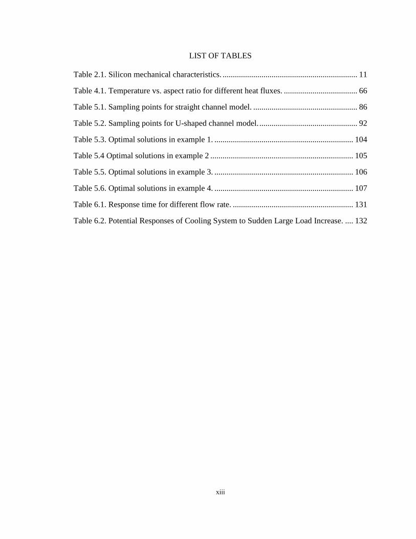
LIST OF TABLES ........................................................................................................... xiii

NOMENCLATURE ........................................................................................................ xiv

Chapter 1 Introduction ........................................................................................................ 1

1.1 Motivation ................................................................................................................. 1

1.2 Literature review on microchannel heat sink ............................................................ 2

1.3 Literature review on data center thermal management systems ............................... 5

1.3.1 Introduction ........................................................................................................ 5

1.3.2 CFD/HT modeling of air cooled data centers .................................................... 7

1.3.3 Study of transient state ....................................................................................... 8

1.4 Dissertation Outline .................................................................................................. 9

Chapter 2 Microchannel Heat Sink Fabrication and Experimental Setup ........................ 11

2.1 Microchannel heat sink fabrication ......................................................................... 11

2.1.1 Wet etching ...................................................................................................... 12

2.1.2 Plasma etching ................................................................................................. 15

vii

2.2 Experimental setup.................................................................................................. 17

2.2.1 Experimental facility ........................................................................................ 17

2.2.2 Calibration and data collection ........................................................................ 19

Chapter 3 Experimental Results for Microchannel Heat Sinks ........................................ 21

3.1 Dimensionless parameter ........................................................................................ 21

3.1.1 Hydraulic parameters ....................................................................................... 21

3.1.2 Heat transfer dimensionless terms ................................................................... 23

3.2 Experimental Uncertainty ....................................................................................... 24

3.3 Experimental Results: ............................................................................................. 26

3.3.1Thermal performance ........................................................................................ 26

3.3.2 Fluid performance ............................................................................................ 36

3.4 Transient response .................................................................................................. 41

Chapter 4 Numerical Simulation and Parametric Study of Microchannel Heat Sink ....... 49

4.1 Numerical model construction ................................................................................ 49

4.1.1 The effect of viscous dissipation ...................................................................... 49

4.1.2 The heat transport mechanism other than forced convection .......................... 50

4.1.3 The physical model .......................................................................................... 52

4.1.4 Mathematical formulation:............................................................................... 55

4.1.5 Model validation .............................................................................................. 56

4.2 Parametric study for straight channel ..................................................................... 59

viii

4.3 Effectiveness of channel with bends ....................................................................... 71

4.4 Effectiveness of channels with branches (Y-shaped channels) .............................. 74

Chapter 5 Design and Optimization of Microchannel Heat Sinks .................................... 80

5.1 Formulation of the design problem ......................................................................... 80

5.2 Curve Fitting ........................................................................................................... 82

5.3 Straight Channel Model .......................................................................................... 84

5.4 U-shape channel model ........................................................................................... 91

5.5 Optimization problems............................................................................................ 97

5.5.1 Example 1 for straight channel model ............................................................. 97

5.5.2 Example 2 for straight channel model ........................................................... 100

5.5.3 Example 3 for U-shape channel model .......................................................... 101

5.5.4 Example 4 for U-shaped Channel model ....................................................... 102

Chapter 6 Data Center Thermal Management ................................................................ 109

6.1 Computer room air conditioning units (CRAC) and cooling system ................... 109

6.2 Model setup ........................................................................................................... 111

6.2.1 The physical model layout ............................................................................. 111

6.2.2 Governing equations ...................................................................................... 112

6.3 CFD/HF modeling results ..................................................................................... 115

6.4 Energy consumption ............................................................................................. 121

6.5 Transient effects and pre-cooling.......................................................................... 130

ix

Chapter 7 Conclusion ...................................................................................................... 139

APPENDIX: Photo masks with different channel configuration patterns ...................... 143

BIBLIOGRAPHY ........................................................................................................... 145

x

LIST OF FIGURES

Figure 2.1. Fabrication and packaging process of microchannel heat sinks (Wet Etching).

........................................................................................................................................... 14

Figure 2.2. SEM micrograph of microchannel after KOH etching. .................................. 15

Figure 2.3. Fabrication and packaging process of microchannel heat sinks (Plasma

Etching). ............................................................................................................................ 16

Figure 2.4. SEM micrograph of microchannel heat sink with plasma etching. ................ 17

Figure 2.5. Schematic drawing of the experimental setup. ............................................... 18

Figure 3.1. Schematic of different microchannel heat sink configurations. ..................... 26

Figure 3.2. Temperature difference vs. flow rate for difference heat sinks. ..................... 27

Figure 3.3. Temperature difference vs. flow rate for straight channel. ............................ 28

Figure 3.4. SEM micrograph of straight channels with different surface roughness. ...... 29

Figure 3.5. Temperature difference vs. flow rate for Y-shaped channel. ......................... 30

Figure 3.6. Temperature difference vs. flow rate for U-shaped channel. ......................... 31

Figure 3.7 Total thermal resitance vs. Reynold number for U-shaped channel ............... 33

Figure 3.8. Total thermal resitance vs. Reynold number for Y-shaped channel. ............. 33

Figure 3.9. Pressure drop vs. Reynolds number for U-shaped channel. ........................... 37

Figure 3.10. Pressure drop vs. Reynolds number for Y-shaped channel. ......................... 38

Figure 3.11. Apparent friction factor Vs. Reynolds number for U-shaped channel. ........ 40

Figure 3.12. Apparent friction factor vs. Reynolds number for Y-shaped channel. ......... 41

Figure 3.13. Temperature vs. time for straight channel. .................................................. 42

Figure 3.14. Temperature vs. time for U-shaped channel................................................ 43

Figure 3.15. Temperature vs. time for serpentine channel. ............................................. 43

Figure 3.16. Response time vs. flow rate for low heat flux. ............................................ 46

Figure 3.17. Response time vs. flow rate for high heat flux. ........................................... 47

Figure 3.18. Response time vs. heat flux for different heat sinks. .................................... 48

Figure 4.1. Free, forced and mixed convection regimes for flow in horizontal tubes.

(Taken from Metais and Eckert). ...................................................................................... 51

xi

Figure 4.2. Sketch of straight microchannel heat sink model. .......................................... 53

Figure 4.3. Sketch of U-shaped microchannel heat sink model. ...................................... 53

Figure 4.4. Sketch of Y-shaped microchannel heat sink model. ...................................... 54

Figure 4.5. Numerical and experimental results comparison for straight channel model. 57

Figure 4.6. Numerical and experimental results comparison for U-shaped channel model.

........................................................................................................................................... 58

Figure 4.7. Numerical and experimental results comparison for Y-shaped channel model.

........................................................................................................................................... 58

Figure 4.8. Thermal resistance vs. length for different aspect ratio. ................................ 61

Figure 4.9. Thermal resistance vs axial distance for different flow rates ( ). ........ 62

Figure 4.10. Pumping power vs flow rate for cases with different aspect ratios. ............. 63

Figure 4.11. Euler number vs. Reynolds number for different aspect ratios. ................... 64

Figure 4.12. Thermal resistances vs. Reynolds number for different aspect ratios. ......... 65

Figure 4.13. Thermal resistances vs. axial distance for constant pumping power. ........... 66

Figure 4.14. Thermal resistances for different coolants at constant flow rate. ................. 67

Figure 4.15. Thermal resistances for different coolants at constant pressure drop. .......... 68

Figure 4.16. Thermal resistances for different heat sink materials at constant flow rate. 69

Figure 4.17. Thermal resistances for different heat sink materials at constant pressure

drop. .................................................................................................................................. 70

Figure 4.18. Sketch of L-bend channel and 90 bend. ....................................................... 71

Figure 4.19. Normalized pressure and streamlines for L bend with different fillets. ....... 72

Figure 4.20. Pumping power vs. Reynolds number for L-bends and 90 bend. ................ 73

Figure 4.21. Thermal resistance vs. Reynolds number for L-bends and 90 bend. ............ 74

Figure 4.22. Temperature distribution in Y-shaped channel. ........................................... 75

Figure 4.23. Velocity distribution in Y-shaped channel (along the flow direction). ........ 76

Figure 4.24. Transverse streamlines for different Re number. ......................................... 77

Figure 4.25. Thermal resistance and non-dimensional pressure drop vs. different channel

length for Y-shaped channel ............................................................................................. 78

xii

Figure 5.1. Iterative process to obtain an acceptable design. ............................................ 81

Figure 5.2. Thermal resistance isosurfaces for straight channel model. ........................... 87

Figure 5.3. Pressure drop isosurfaces for straight channel model. ................................... 89

Figure 5.4. Maximum temperature isosurfaces for straight channel. ............................... 90

Figure 5.5. Thermal resistance isosurfaces for U-shaped channel. ................................... 93

Figure 5.6. Pressure drop isosurfaces for U-shaped channel. ........................................... 95

Figure 5.7. Max. Temperature isosurfaces for U-shaped channel. ................................... 96

Figure 5.8. Pareto frontiers of example 1. ........................................................................ 99

Figure 5.9. Pareto frontiers of example 2. ...................................................................... 101

Figure 5.10. Pareto frontiers of example 3. .................................................................... 102

Figure 5.11. Pareto frontiers of example 4. .................................................................... 103

Figure 6.1. Schematic drawing of the CFD data center model. ...................................... 112

Figure 6.2. Temperature distribution in the data center with 25% utilization. ............... 116

Figure 6.3. Temperature distribution in the data center with 50% untilization. ............. 117

Figure 6.4. Streamlines for utilization 50%, are operating. .............................. 119

Figure 6.5. Temperature distribution with untilization 75% and 100%. ........................ 120

Figure 6.6. The impact of outside temperature on energy consumption (Janurary, Seattle).

......................................................................................................................................... 124

Figure 6.7. The impact of outside temperature on energy consumption (Janurary,

Princeton). ....................................................................................................................... 126

Figure 6.8. The impact of outside temperature on energy consumption (August,

Princeton). ....................................................................................................................... 128

Figure 6.9. Transient temperature distribution in the data center for scenario 2. ........... 135

Figure 6.10. Temperature vs. time for different scenarios. ............................................. 136

Figure 6.11. Temperature in the data center vs. different cooling responses. ................ 138

xiii

LIST OF TABLES

Table 2.1. Silicon mechanical characteristics. .................................................................. 11

Table 4.1. Temperature vs. aspect ratio for different heat fluxes. .................................... 66

Table 5.1. Sampling points for straight channel model. ................................................... 86

Table 5.2. Sampling points for U-shaped channel model. ................................................ 92

Table 5.3. Optimal solutions in example 1. .................................................................... 104

Table 5.4 Optimal solutions in example 2 ...................................................................... 105



Table 6.1. Response time for different flow rate. ........................................................... 131

Table 6.2. Potential Responses of Cooling System to Sudden Large Load Increase. .... 132

xiv

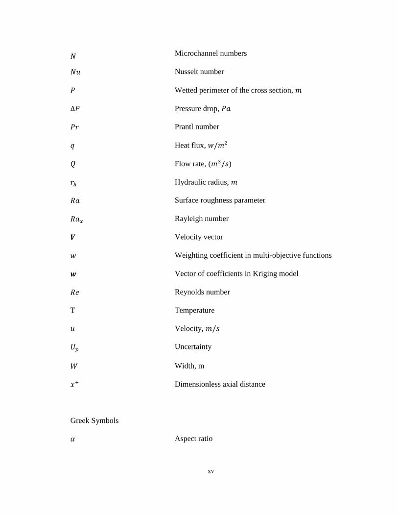
NOMENCLATURE

Specific heat capacity,

Covariance tensor

COP coefficient of performance

Hydraulic Diameter,

Normal basis

Parametric model using Kriging

Vector of responses

Fanning friction factor

Apparent fanning friction factor

pF Fractional open area of the perforated tile

Body force,

thi Inequality constraint

Turbulence kinetic energy

Heat transfer coefficient

H Height, m

Thermal conductivity,

Coverage factor

K Flow resistance factor

Number of sampling points

xv

Microchannel numbers

Nusselt number

Wetted perimeter of the cross section,

Pressure drop,

Prantl number

Heat flux,

Flow rate, ( )

Hydraulic radius,

Surface roughness parameter

Rayleigh number

Velocity vector

Weighting coefficient in multi-objective functions

Vector of coefficients in Kriging model

Reynolds number

T Temperature

Velocity,

Uncertainty

Width, m

Dimensionless axial distance

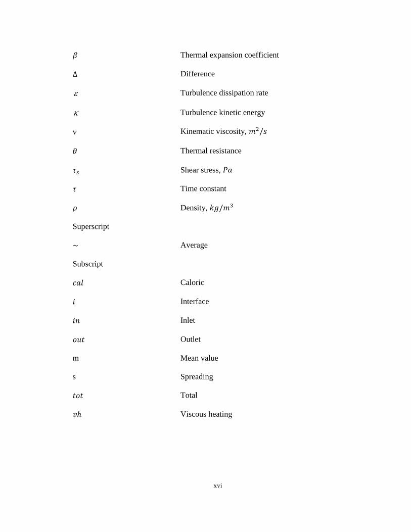
Greek Symbols

Aspect ratio

xvi

Thermal expansion coefficient

Difference

Turbulence dissipation rate

Turbulence kinetic energy

Kinematic viscosity,

Thermal resistance

Shear stress,

Time constant

Density,

Superscript

Average

Subscript

Caloric

Interface

Inlet

Outlet

m Mean value

s Spreading

Total

Viscous heating

1

Chapter 1 Introduction

1.1 Motivation

Electronic devices, reaching into every aspect of modern living, are becoming more and

more sophisticated and highly compact. This trend leads to increasingly high heat density

generated by electric current. The heat flux from the surface of an electronic chip

increased from approximately 102 to 10

7 watts per unit meter square. For large scale

electronic systems, high heat flux is also becoming a concern due to the rising power

density. In order to avoid the malfunctions of electronics and to ensure the reliability of

the electronic systems, substantial research work has been done to explore more effective

cooling techniques to keep up with the development pace of new electronic equipment

and large electronic systems.

The main purpose of the current study is to investigate thermal performance of electronic

cooling system at different scales. Micro-scale electronic cooling was studied through

experiments and numerical simulation. Different configurations of microchannel heat

sinks were investigated. Optimized solutions for single-phase liquid flow in microchannel

heat sinks were found. Large-scale electronic cooling was investigated to address the

thermal challenges in data centers with varying heat load at both steady and transient

states.

2

1.2 Literature review on microchannel heat sink

A heat sink consisting of multiple microchannels with liquid flow is believed to be a

promising cooling method for high heat dissipation electronic chips due to the relatively

high heat capacity and heat removal efficiency offered by liquids in contrast to air

(Tuckermann and Pease 1981). Previous research works on microchannel fluid flow and

heat transfer have involved both computational and experimental methods (Kandlikar

2003, Wei and Joshi 2004, Zhang et al 2005, Steinke et al 2006). It is noticed that, due to

the fabrication process, the silicon base of microchannels usually has non-circular and

mostly rectangular cross sections.

The majority of the references cited in literature use the Navier-Stokes equation to

analyze the microscale fluid system numerically. Since convective heat transfer in

rectangular channels is critical in macro-scale design, early studies on micro-scale

rectangular channels also focused on convective heat transfer (Tso and Mahulikar 1998,

Harms et al 1999). However, unlike the macro-scale channels, the ratio of fin and channel

width as well as the ratio of the silicon substrate thickness and the channel depth is not

negligible in micro-scale systems. Therefore, researchers started to realize that

conduction plays an importance role in the overall heat transfer (Marabzan 2004, Sharath

2006). Combined conduction and convection, or conjugate heat transfer, needs to be

considered for numerical analysis for micro-scale cases. Fedorov and Viskanta (2000)

used classical theory to analyze conjugate heat transfer in a three dimensional

3

microchannel heat sink. Husian and Kim (2007) solved the Navier-stokes and the energy

equations to study the conjugate heat transfer and fluid flow in microchannels, and also

used the multiobjective method to optimize the ratio of channel width to depth. Li and

Peterson (2004) provided a detailed temperature and heat flux distribution using a

simplified three dimensional conjugate heat transfer model (2D fluid flow and 3D heat

transfer). The effect of temperature dependence has also been studied (Li et al 2007).

Model with varying thermal properties generated results closer to experiments than

model with constant thermal properties.

The fabrication process of microchannels introduces local variations in channel properties

due to the surface roughness or differences in surface chemical composition. Modeling

these changes continues to be a challenge (Papautsky et al 1999, Mala et al 1997). Hence,

experimental investigation is important in understanding the heat transfer and fluid

dynamics in microchannels. Tuckerman and Pease (1981) were the first to set up

experiments on a microchannel heat sink, which provided the precedent for many

experimental studies. Steinke and Kandlikar et al (2006) presented details of

an experimental facility that was capable of accurately investigating the performance of a

microchannel heat sink with different geometries by including the experimental

uncertainty. Wei and Joshi (2004) designed a double-layered microchannel heat sink,

which reduced half of the pressure drop under constant flow rate. They also studied

sidewall velocity profiles in microchannels using micro-PIV. It was a significant

improvement in term of reducing the pumping power, but the thermal resistance was not

very sensitive to the number of layers. Therefore, the thermal performance was not

4

improved significantly. Zhang et al. (2005) applied actual electronic packages (flip chip

ball grid array packages) as heat source on the bottom of the heat sink instead of

simulated heaters in their study. The junction temperature was measured and the

experimental results matched the analytical prediction quite well.

Other than single-phase liquid flow, there were also substantial studies focusing on

boiling flow in mirochannels. It is more complex experimentally and numerically to

capture the phase change. Haritchian and Garimella (2008) performed an experiment on

two-phase heat transfer in microchannel heat sinks for high heat fluxes. Zhang et al (2002)

recorded the pressure and wall temperature distribution during the phase change. Even

though it is important to report and visualize the boiling flow in microchannel, applying

two phase flow for electronic cooling may not be necessary if liquid cooling is effective.

All experiments till date have mostly explored ways to improve the thermal performance

of the straight rectangular microchannel heat sink by optimizing the aspect ratio of the

straight rectangular microchannels and its fins, in order to increase the convective heat

transfer by the coolant. However, to the best of our knowledge, little work was done on

the single-phase liquid multi-microchannel heat sinks with bends and branches. Xiong

(2007) and Wang (2009) studied the flow behavior in the U-shaped and serpentine

microchannels, but the heat transfer characteristics were not included.

5

The design optimization of microchannels is another important aspect in the study of

micro-cooling systems. Husain and Kim (2009) solved the Navier-Stokes and the energy

equations to study the conjugate heat transfer and fluid flow in microchannels. They used

the multi-objective method to optimize the ratio of channel width to depth. Even though

there were substantial studies on the design optimization of the thermal system (Lin

2010), most of the optimization studies for microchannel electronic cooling were based

on the experimental results, and therefore were limited by the number of samples and the

experimental data range.

In the current study, different configurations were tested through experiments: straight

channels, U-shaped channels, Y-shaped channels and serpentine channels. The objective

of this study is to investigate the heat transfer characteristics of multi-microchannel heat

sinks. The simulation results from the conjugate heat transfer model that considered both

conduction and convection appeared to match the experimental data fairly well. The

numerical models were then used to conduct a parametric study, based on which an

optimization problem was formulated and investigated.

1.3 Literature review on data center thermal management systems

1.3.1 Introduction

Data centers are the foundation of many IT related operations for companies of different

industries all over the world. A data center holds computer servers, telecommunications

6

equipment, data storage systems and many other devices. It is common for a large data

center to house more than thousands of server racks with 20~40 servers per each rack.

The server chips, which may contain several millions of transistors, will generate a

significant amount of heat. The increase of the surface heat flux of electronic chips

consequently leads to a high heat density in data centers. Overheating can cause

malfunction of servers, which may cost thousands or millions of dollars per minute

downtime.

The energy consumed in a data center includes cooling, uninterrupted power supply

losses, computer loads and lighting. It was reported that the HVAC system (including

chiller and pump) of a typical data center takes up to 54% of the total energy

consumption (Tschudi et al 2003). At the same time, the amount of cooling air used in

most data centers is 2.5 times more than the required amount (Karki et al 2003). Google

has invested substantial resources in reducing their data center power use, and reports a

Power Usage Effectiveness (PUE) in the 1.1~1.35 range (Abtes et al 2011). Most data

centers use the under-floor plenum below a raised floor to supply cold air to the room.

The cold air is delivered from the computer room air conditioner (CRAC) units into the

plenum, from where it is introduced into the data center via perforated tiles. By placing

the perforated tiles in front of each server rack, it is possible to supply high speed cold air

to each rack. The cold air is then distributed to each server by the fan. The advantage of

this design is that the solid floor tiles are removable and can be replaced by the perforated

tiles. Hence, if the server racks (heat source) layout changed, the perforated tile location

can be changed accordingly. This design can meet the needs for most of the data centers.

7

If the power load is increased, the extra heat dissipated can be removed with an

increasing flow rate or with a lower inflow temperature.

Even though the existing design of the under floor plenum with the perforated tiles has

the cooling capacity of the current heat load, the cooling system has to meet the needs of

the next generation’s electronics due to the rapid development of semiconductor industry.

Ten percent of the equipment in a data center is replaced each month (International

Technology Roadmap for Semiconductors 2008). Energy consumption becomes a bigger

concern with the existing cooling system design and the increasing cooling demands. A

large potential of cost and energy saving has been realized and the concept of “green data

center” has been proposed.

1.3.2 CFD/HT modeling of air cooled data centers

Computation Fluid Dynamics/Heat Transfer modeling is the most practical scientific

approach to predict the airflow and temperature distribution in the data center, since it

provides comprehensive information to the study of HVAC system efficiency. The

thermal management of data centers has only been carefully investigated for the past

decade, due to the lack of powerful computing solutions to a large turbulence model.

More CFD tools are accessible now to the study of the fluid dynamics and heat transfer

inside of a data center.

8

Throughout the data center industry, the study of energy efficiency has become one of the

research priorities (Patterson 2008, Greenberg et al 2006). Based on the assumption of

uniform pressure distribution above the raised floor, Karki, Radmehr and Patankar (2003)

applied a CFD model to simulate the velocity and flow rate of a real-life data center. The

calculated results showed a good agreement with their measured data. Schmidt (2004)

presented measured data of airflow rates for a number of different floor layouts for

raised-floor data center, where some of the experimental cases were picked out and

simulated by a CFD model which showed a good agreement. Schmidt et al (2008)

pointed out that the numerical simulation was over estimating the hot and cold spot of the

real data center, which may be caused by the simplification to the model especially the

simplified representation of the server racks.

1.3.3 Study of transient state

Electronic cooling problems have always been considered as steady-state conditions.

However, the maximum heat load usually appears at the start or the shutdown instance of

a single electronic chip. For data centers, the transient state is also important since the

maximum heat load may rise for certain time period. For instance, the internet takes more

traffic after 5pm when people get off work, and it causes the servers to suddenly run from

idle state to full load state. The heat dissipated from a server may increase from 150W to

300W correspondingly. The temperature of the equipment and server room starts to

increase dramatically. The response time of the HVAC system becomes critical in this

case. The transient-state study of electronic cooling process is lacking due to the

9

complexity of simulating combined convection, radiation and interface conditions. The

current study addresses the transient state to better represent the real-world data center

conditions and obtain the response time of the HVAC system.

1.4 Dissertation Outline

Chapter 1 explains the importance of cooling for electronics in both micro-scale and large

scale systems. For electronic chip cooling, the single-phase liquid-flow microchannel

heat sinks are introduced. Conventional scale turbulence model is introduced for data

center cooling system. Some previous works are reviewed briefly and the objectives of

the study are stated.

Chapter 2 describes the experimental configuration. The microchannel heat sink device

design and fabrication process are introduced. The experimental setup, the equipment

calibration and the uncertainty analysis are presented.

Chapter 3 presents the experimental results. Both steady state and transient time response

results are included. The thermal performance and fluidic performance of heat sinks with

different configurations are compared and discussed.

10

Chapter 4 presents the numerical model setup and validation. The assumptions of the

numerical studies are reviewed. The numerical predictions, including different

parameters and their influence on the heat sink performance are investigated in detail.

Chapter 5 formulates an optimization problem based on the parametric modeling results

with the numerical models developed in chapter 4. A multi-objective optimization

problem is solved with the Pareto frontier presented and discussed.

Chapter 6 deals with the thermal management for data centers. The management strategy

of the thermal system to respond effectively to a sudden load increase and avoid

performance degradation is discussed. Meanwhile, the energy consumption and cost

reduction is investigated with the state of the art data center cooling systems.

Chapter 7 presents the conclusions of this study. Different design systems are

summarized with suggestions. Possible future interests and suggestions are listed for the

study of multi-scale electronic cooling.

11

Chapter 2 Microchannel Heat Sink Fabrication and Experimental Setup

2.1 Microchannel heat sink fabrication

Fabrication and packaging process is the first and also a very important step for the

experimental setup. There are several materials that can be used as for the microchannel

heat sink fabrication including diamond, iron, silicon, steel, stainless steel, and aluminum.

Single crystal silicon is being employed in modern fabrication because of its well-

established electronic properties and its excellent mechanical properties. Many

microfabrication technologies have been developed using single-crystal silicon for its

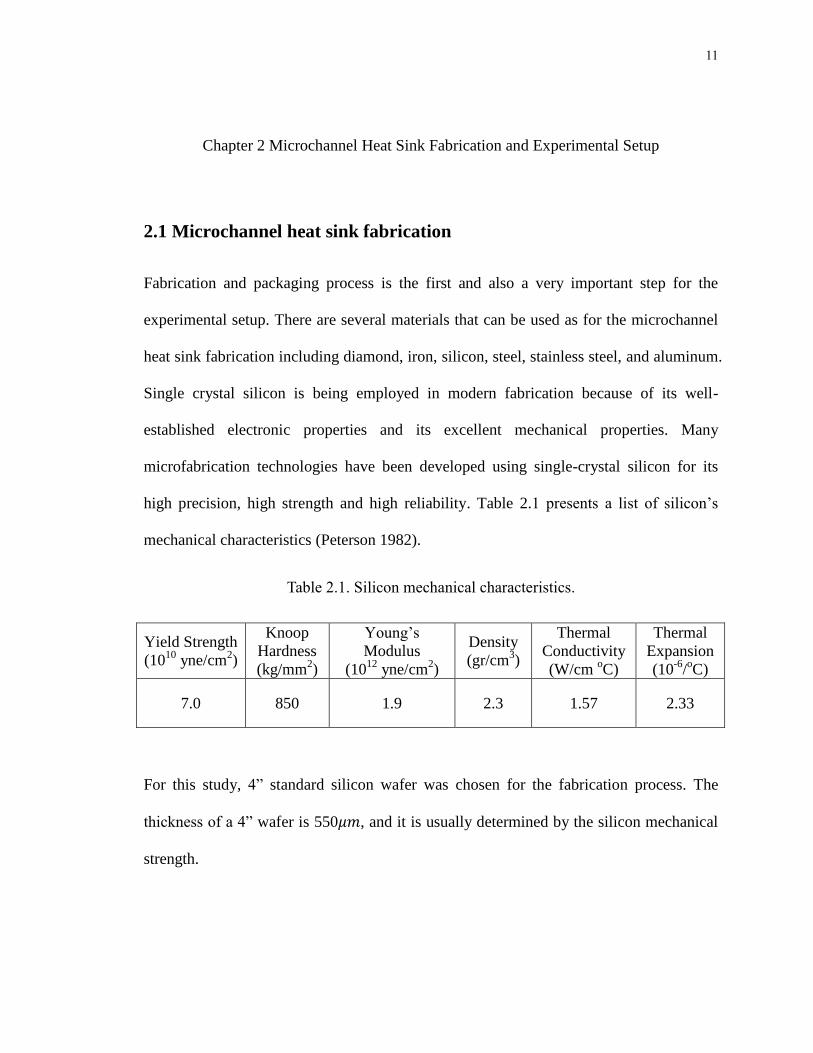
high precision, high strength and high reliability. Table 2.1 presents a list of silicon’s

mechanical characteristics (Peterson 1982).

Table 2.1. Silicon mechanical characteristics.

Yield Strength

(1010

yne/cm2)

Knoop

Hardness

(kg/mm2)

Young’s

Modulus

(1012

yne/cm2)

Density

(gr/cm3)

Thermal

Conductivity

(W/cm oC)

Thermal

Expansion

(10-6

/oC)

7.0 850 1.9 2.3 1.57 2.33

For this study, 4” standard silicon wafer was chosen for the fabrication process. The

thickness of a 4” wafer is 550 , and it is usually determined by the silicon mechanical

strength.

12

Two different methods were used to create the microchannels: wet etching and dry

etching. The advantages and disadvantages of both methods are well-known. The most

important ones for micromachining are as follows: Wet etching is usually isotropic,

which can have a selectivity that depends on crystallographic direction, and can be very

selective over masking and underlying layers. Plasma etching (dry etching) can be

vertically anisotropic, allowing the patterning of narrow lines. Hence many high aspect

ratio MEMs devices are made by dry etching. Both methods were used in the experiment.

Hence both dry etching and wet etching will be introduced in this chapter.

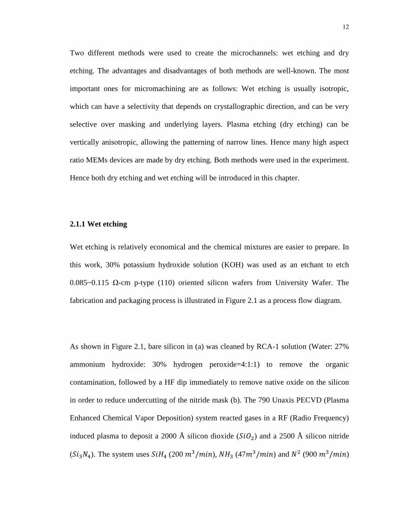
2.1.1 Wet etching

Wet etching is relatively economical and the chemical mixtures are easier to prepare. In

this work, 30% potassium hydroxide solution (KOH) was used as an etchant to etch

0.085~0.115 Ω-cm p-type (110) oriented silicon wafers from University Wafer. The

fabrication and packaging process is illustrated in Figure 2.1 as a process flow diagram.

As shown in Figure 2.1, bare silicon in (a) was cleaned by RCA-1 solution (Water: 27%

ammonium hydroxide: 30% hydrogen peroxide=4:1:1) to remove the organic

contamination, followed by a HF dip immediately to remove native oxide on the silicon

in order to reduce undercutting of the nitride mask (b). The 790 Unaxis PECVD (Plasma

Enhanced Chemical Vapor Deposition) system reacted gases in a RF (Radio Frequency)

induced plasma to deposit a 2000 Å silicon dioxide ( ) and a 2500 Å silicon nitride

( ). The system uses (200 ), (47 ) and (900 )

13

For the deposition. The corresponding operating temperature, pressure and RF are

300°C, 900 mTorr, and 19W, respectively. The deposition rate is 1000 Å every three

minutes. For the deposition, the available gases are (160 ) and

(720 ). The operating temperature, pressure and RF are 250°C, 900 mTorr, and

25W, respectively. The deposition rate is 100 Å/min. Buffered oxide etch 7:1 was

used to open window of silicon nitride (d) after conventional Ultraviolet (UV)

photolithography defines the microchannel pattern on the photo resist (c). The silicon

wafer was then dipped into AZ400T solution (e) for half an hour to remove the rest of the

photo resist before it dissolved in KOH solution (f). A magnetic stirrer was used to

agitate the KOH solution to prevent the etch rate variation from the top to the bottom.

10%~15% isopropanol was added to KOH solution to improve the etch uniformity. A

PDMS layer is bonded on top the silicon microchannels after treating with oxygen

plasma at 200 W for 15 sec at room temperature (h). Openings were punched in the

PDMS for fluid connections. Figure 2.2 shows the SEM of the fabricated microchannel.

KOH etching is orientation dependent and this anisotropic etching scheme allows

tailoring of sidewall profiles. However, Microchannel fabricated on (110) oriented silicon

wafer cannot be scribed by diamond pens as the second crystal cleavage plane is not

perpendicular to the primary cut, but has a 70.5º angle.

There are two ways to separate these samples. First, the samples on a silicon wafer can be

separated along its self-cleavage direction. The disadvantage of this method is that the

surface area of the heat sink will be changed. The other is to create pre-etched grid lines

and etch in KOH solution to ensure the device can be separated out safely along those

14

grid lines [Dwivedi et al 2000]. The overall heat sink dimensions are better controlled

this way. The latter method is adopted in this study.

Figure 2.1. Fabrication and packaging process of microchannel heat sinks (Wet Etching).

15

Figure 2.2. SEM micrograph of microchannel after KOH etching.

Wet etching provides a relatively economical method to fabricate microchannel heat

sinks when plasma etching equipment is not available. The down side of the wet etching

process is the challenge in controlling the undercutting (figure 2.2) and sidewall profile,

which tends to be more controllable with dry etching. Moreover, Plasma etching is also

more efficient.

2.1.2 Plasma etching

Plasma etching was also used in the experiment to fabricate complicated structures. The

wafer preparation for dry etching is easier since it includes less steps compare with wet

etching. The cleaning process is the same, then followed by photolithography process

(Figure 2.3). AZ1518 were used as mask to protect fins from etching. The SAMCO

International RIE800iPB is used for dry etching process. It is a state of the art inductively

coupled plasma etcher. The entire 4” silicon wafer were etched in the etcher and got a

depth of 175 microns.

16

Figure 2.3. Fabrication and packaging process of microchannel heat sinks (Plasma

Etching).

17

Multichannel heat sink with bifurcation

Multichannel heat sink with counter flow

Figure 2.4. SEM micrograph of microchannel heat sink with plasma etching.

2.2 Experimental setup

2.2.1 Experimental facility

For experiments, a commercial miniature Kapton heater from Minco was attached using a

high conductive epoxy underneath the microchannel heat sink to simulate the heat

released by an electronic chip. The heat flux provided by the heater was controlled via

regulating electrical current and voltage of a DC power supply. 4 T-type thermocouples

from Omega (Model number: 5TC-TT-T-36-36) were attached on the heater to measure

18

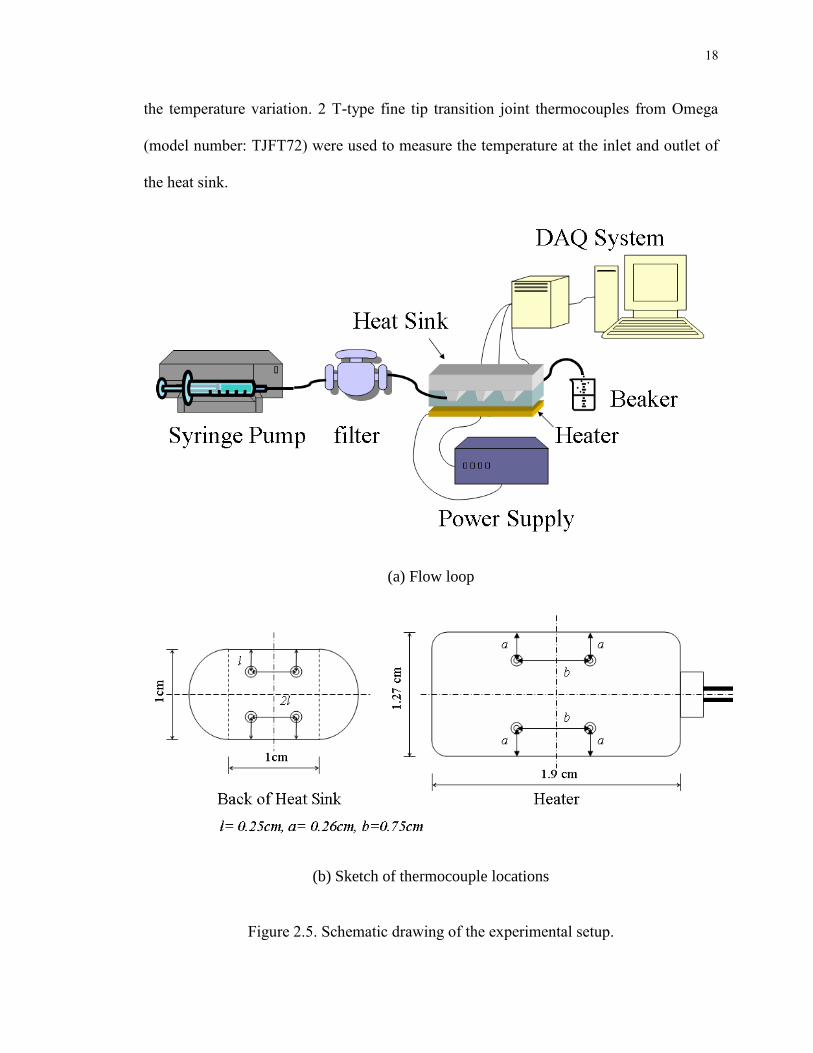
the temperature variation. 2 T-type fine tip transition joint thermocouples from Omega

(model number: TJFT72) were used to measure the temperature at the inlet and outlet of

the heat sink.

(a) Flow loop

(b) Sketch of thermocouple locations

Figure 2.5. Schematic drawing of the experimental setup.

19

All the temperature data were collected by the data acquisition system including SCXI

system, which consists of SCXI-1000 chassis, SCXI-1100 multiplexer module and the

SCXI 1300 terminal block. The SCXI system is used to connect the measurement devices

to PCI-6040E DAQ card from National Instrument. A pressure transducer from

ASHCROFT (model number: KITMO215F2100) was installed at the inlet of the heat

sink to measure the pressure drop. The pressure transducer is then connected to BNC2120

to send data to the computer. The DAQ software is LabVIEW.

Distilled water was used as the coolant due to its large heat capacity (4186 J/kg·K, one of

the best among liquid). As showed in figure 2.5, the PHD 2000 Infuse/Withdraw syringe

pump from Harvard Apparatus was used to drive the flow. The programmable aspects of

the syringe pump also allow the usage of the pump as a flow meter and a valve since

specific flow rates can be dialed in for continuous measurements. A filter with 1

micrometer mesh element was used after the syringe to remove any residual impurities

suspended in the cooling water.

2.2.2 Calibration and data collection

All the thermocouples were carefully calibrated in a water bath by using a 6-points

calibration method. Since the coolant liquid is water, the operating range for the

experiments was expected from 0˚C to 100˚C. All the calibration data were recorded and

a piecewise linear curve fit was formed. The thermocouples show ±0.5˚C of each other

20

when measuring a known temperature after calibration was performed, which means that

the thermocouples may have an accuracy of ±0.5˚C.

All of the multi-microchannel heat sinks have the same surface area (inlet and

outflow reservoirs are not included). The syringe pump was turned on before the DC

power supply and we waited to let the system run for a while to ensure open bubble-free

channels with no leakage in the test system. Then we turned on the power supply, and

started recording data.

Several different heat sink configurations were designed and fabricated. The photo masks

with different channel configuration patterns can be found in the appendix A. The

experimental results with the facility introduced above will be presented and discussed in

chapter 3.

21

Chapter 3 Experimental Results for Microchannel Heat Sinks

This chapter will present the experimental results obtained with the experimental set up

introduced in the previous chapter. The dimensionless terms used in this study will be

introduced first. Then the experimental measurements uncertainties will be evaluated.

The experimental results with different geometry configurations will be presented and

discussed.

3.1 Dimensionless parameter

3.1.1 Hydraulic parameters

There are several commonly used dimensionless parameters in fluid dynamics and heat

transfer to describe the pressure drop and heat transfer characteristics, which allowed

researchers study and compare the results from different literatures more efficient and

easier. Definitions of dimensionless parameters used in this paper are as follows (Shah

and London, 1978):

a) Reynolds number Re

Re huD

(3.1)

where the hydraulic diameter is defined as: .

22

b) Fanning friction factor f:

Fanning friction factor is defined as the ratio of wall shear stress to the flow kinetic

energy per unit volume :

2 / 2

xx

m

fu

(3.2)

The equation above represents the local fanning friction factor. The mean (flow length

average) fanning friction factor in the hydrodynamic entrance region is defined as:

20

1

/ 2

xm

m x

m

f f dxx u

(3.3)

For the purpose of engineering application, for constant density and constant velocity

profile, the pressure drop for the singly connected channel with constant cross section

area can be presented by the apparent fanning friction factor:

*

2 / 2app

m h

P xP f

u r

(3.4)

is calculated based on the total pressure drop from x=0 to x. Both the skin friction

and the momentum rate change are taken into account in the hydrodynamic entrance

region. is also used in this study to represent the pressure drop in chapter 4. For a

fully developed flow in a channel with channel length L, the equation becomes:

2 / 2m h

P Lf

u r

(3.5)

For fully developed laminar flow in rectangular channel, the number is a function of

the aspect ratio:

23

2 3 4 5Re 24*(1 1.3553 1.9467 1.7012 0.9564 0.2537 )f ( 3 . 6 )

c) Dimensionless axial distance

The dimensionless axial distance in the flow direction is defined as:

/ Rehx x D (3.7)

The dimensionless axial distance corresponding to hydrodynamic developed region is

smaller than 0.1 for rectangular channels. The hydrodynamic entrance length becomes

longer as the channel aspect ratio increases (Wiginton and Dalton, 1970).

3.1.2 Heat transfer dimensionless terms

a) The fluid bulk mean temperature is defined as:

1m c

Ac m

T utdAA u

(3.8)

b) The heat transfer coefficient h

The most operationally convenient parameter to describe the heat transfer rate is heat

transfer coefficient .

The average heat transfer coefficient is defined as:

24

''

0

1

( )

x

x

w m

qh dx

x t t

(3 .9)

For linear problems, is independent of the temperature difference.

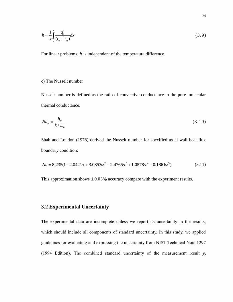
c) The Nusselt number

Nusselt number is defined as the ratio of convective conductance to the pure molecular

thermal conductance:

/

mm

h

hNu

k D (3 .10)

Shah and London (1978) derived the Nusselt number for specified axial wall heat flux

boundary condition:

2 3 4 58.235(1 2.0421 3.0853 2.4765 1.0578 0.1861 )Nu (3.11)

This approximation shows accuracy compare with the experiment results.

3.2 Experimental Uncertainty

The experimental data are incomplete unless we report its uncertainty in the results,

which should include all components of standard uncertainty. In this study, we applied

guidelines for evaluating and expressing the uncertainty from NIST Technical Note 1297

(1994 Edition). The combined standard uncertainty of the measurement result y,

25

designated by uc(y) and taken to represent the estimated standard deviation of the results,

is the positive square root of the estimated variance u2c(y) obtained from:

12 2 2

1 1 1

( ) ( ) ( ) 2 ( , )N N N

c i i j

i i j ii i j

f f fu y u x u x x

x x x

(3.12)

This propagation of uncertainty is used to evaluate uncertainty of a result which depends

on several variables, each with its own uncertainty.

An expanded uncertainty is defined as

( )p p cU k u y (3.13)

Where kp is a coverage factor. Here, kp=2 defines an interval having a level of confidence

of approximately 95 percent. The measurement Y estimated by y is commonly written as:

pY y U (3.14)

For example, the hydraulic diameter is defined as:

4

2( )

c ch

c c

W HD

W H

(3.15)

The uncertainty of is defined as:

2 2 2 2( ) ( ) ( ) ( )hD a a d d

h

U U U U U

D a a d d a d

(3.16)

26

3.3 Experimental Results:

3.3.1Thermal performance

a. Straight Channel

b. Y-shaped Channel

c. U-shaped Channel

d. Serpentine Channel

Figure 3.1. Schematic of different microchannel heat sink configurations.

27

As mentioned in the previous chapter, there are several different heat sinks fabricated

with various configurations. Four major ones are shown in figure 3.1. In the experiment,

the heater was attached on the bottom of the heat sink. The distilled water at room

temperature will be pumped into the microchannel heat sink, takes away the heat, and

exit from the outlet to a beaker.

Figure 3.2. Temperature difference vs. flow rate for difference heat sinks.

Four thermocouples were attached on top of the heater to record the temperature data.

The heater temperature was calculated based on the average readings from the four

thermocouples. The temperature difference between the inlet coolant and heater are

shown in figure 3.2. All the heat sinks devices presented in this figure were fabricated on

the same silicon wafer (except the straight channel with high Ra number) using plasma

etching. Hence, the channel heights are the same for all the cases. In general, the

28

temperature difference is decreaseing as the flow rate increases for difference heat sinks

as expected.

Figure 3.3. Temperature difference vs. flow rate for straight channel.

Figure 3.3 shows the temperature difference for the straight channel with different

surface roughness. The surface roughness parameter Ra is the arithmetical mean

roughtness obtained with a surface profilometer with randomly sampled channel area

along the flow direction. The straight channel heat sink pictures with different Ra

numbers taken by SEM are shown in figure 3.4. Compare with a smooth-wall flow(Ra=4),

the channle with high Ra number (Ra=33) has negative effect on removing heat. The red

curve shown in figure 3.3 is flat, showing that increasing the flow rate can not change the

thermal performance when the Ra number is high. This results suggest that it is important

to control the channel surface finishing during the fabrication process, and reduce the

29

bottom and side walls rougthness will help improve the thermal performance of the

deivce.

(a) Ra=4

(b) Ra=33

Figure 3.4. SEM micrograph of straight channels with different surface roughness.

30

Figure 3.5. Temperature difference vs. flow rate for Y-shaped channel.

Figure 3.5 shows the temperature difference for different channels with branches. The

blue diamond marker and the red triangle marker represent heat sink with two branches

(the Y-shaped channel shown in figure3.1 (b)). The first one (blue curve) has an inlet

channel width of , then one channel splits into two channels of width .

The second one (red curve) has an inlet channel width of , and then it reduces

to . Another heat sink shown as black rectangle markers in the figure has three

branches. The channel width is first reduced from to , and then

becomes as it goes to the exit. Y-shaped channel with a larger hydraulic diameter

shows the best cooling effect among the three. The temperature difference becomes

larger as the channel size shrinks. This might be caused by the poor convection happened

31

at the corners, as the flow is trapped at the corners when separating to narrow channels

branches.

The temperature difference for the U-shaped channel is shown in figure 3.6. The

temperaeture difference for straight channel is also plotted as a reference. The U-shaped

channel shows a significant better cooling effect compare with the straight channel within

current experimental range. The 180º bend of the U-shaped channel will result a better

flow mixing as well as axial heat conduction enhancement, which contribute to low

heater tempreature.

Figure 3.6. Temperature difference vs. flow rate for U-shaped channel.

The total thermal resistance will be used to evaluate the thermal performance of the liquid

cooled microchannel heat sinks. The modified total thermal resistance is defined as:

32

httot

TA

q

(3.17)

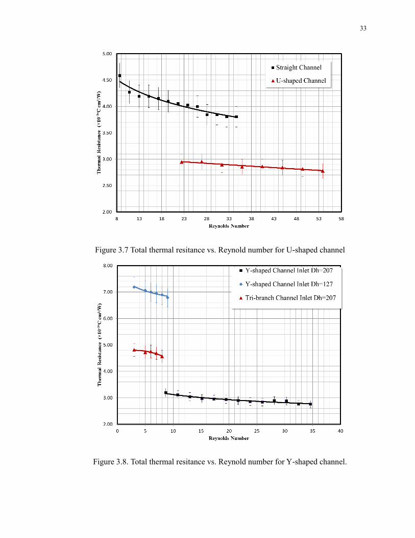
The total thermal resistances Vs Reynolds number for different configurations is shown

in figure 3.7 and figure 3.8.The thermal resistance becomes smaller as the Reynolds

number increases. But the decreasing rate of the thermal resistance gets slower as the Re

increases. At the laminar flow region, the thermal performance of the heat sink will reach

certain value with a fixed geometry, and it cannot be further improved by simply

increasing the flow rate. The configurations that have lower thermal resistance among all

the tested devices are the U-shaped channel, Y-shaped channel (with larger hydraulic

diameter) and the straight channel.

The total thermal resistance of the system is composed of five components (Tuckerman,

1984),

tot s b cal i c (3.18)

Each term will be explained in the following section.

33

Figure 3.7 Total thermal resitance vs. Reynold number for U-shaped channel

Figure 3.8. Total thermal resitance vs. Reynold number for Y-shaped channel.

34

The thermal spreading resistance s is the thermal resistance from the individual heat

generating devices. In the real electronic cooling application, it is due to thermal

spreading of the discrete heat source such as the integrated circuit feature or gate. In our

application, it is heating stripe in the miniature heater. For a square heat source, the

thermal spreading resistance is calculated as(Tuckerman, 1984):

0.56 /s ht h jA k L (3.19)

For straight channel in our study, the total heat transfer area is , and the lead

wire length is 77.42cm, with a thermal conductivity of 35.3 W/mK. This leads to

value of . The temperature rise due to the thermal spreading should

decrease as the level of the circuit integration increases. Therefore, this value will be even

smaller as the heat flux increases.

The second component b is due to heat conduction through the semiconductor substrate,

which is calculated as:

s htb

s

t A

k A (3.20)

where st is the semiconductor substrate thickness, and A is the substrate area. For our

experiment, the thickness of the heater is . b according to equation (3.20) is

0.0002 . It is a fairly small number. Furthermore, the substrate thickness for the

electronic chip is getting thinner and thinner, which will lead to an even smallerb .

35

The third component cal is the caloric thermal resistance due to the heating of the fluid

as it absorbs energy passing through the heat sink. It is calculated as:

1b

pC Q

(3.21)

The higher flow rate, the lower cal will be. For example, for 10 ml/min of water, the

caloric thermal resistance will be 0.004ºC/Wm, which is very small.

The fourth component is the thermal resistance associated with the IC/heat sink interface

i , which is calculated as:

ii

i

t

k A (3.22)

where it is the thickness of the interface material, and

ik is the thermal conductivity of the

interface material. This term is also called contact resistance in this study. If the

microchannel heat sink and the heater are in full contact, this term is zero. In this

experiment, the microchannel heat sink is not in full contact with the heater because of

the attached thermocouples. It also depends on the flatness of heater surface. The

diameter of the thermocouple is 0.13mm, which means that the gap between the heater

and the heat sink is at least 0.13mm. Other than the contact region thickness, the interface

material will also have a great influence on i . For example, the straight channel heat

sink with high conductivity paste will lead to contact resistance as high as 0.002

, which is 45% of the total thermal resistance. Hence, it is very important to reduce the

36

contact resistance for high heat flux applications. Note that this term can be eliminated

entirely by integrating the heat sink on the heat generating circuits.

The last component is the convective thermal resistance c between the heat sink and

coolant. It also includes the thermal resistance of heat conduction in the fin. This is the

primary thermal resistance in electronic cooling application and the most difficult one to

minimize.

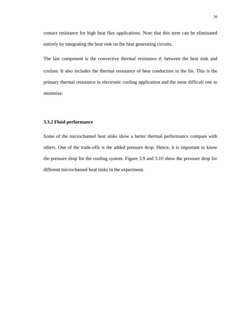
3.3.2 Fluid performance

Some of the microchannel heat sinks show a better thermal performance compare with

others. One of the trade-offs is the added pressure drop. Hence, it is important to know

the pressure drop for the cooling system. Figure 3.9 and 3.10 show the pressure drop for

different microchannel heat sinks in the experiment.

37

Figure 3.9. Pressure drop vs. Reynolds number for U-shaped channel.

38

Figure 3.10. Pressure drop vs. Reynolds number for Y-shaped channel.

For the straight microchannel heat sink, the overall pressure drop has six components.

The flow from the inlet tube will turn 90 degrees and go to the reservoir. As it flows to

each microchannel, it experiences a sudden contraction which causes the flow to separate

and undergo an irreversible free expansion. In the core, the liquid flow will have skin

friction and a density change due to heating. As it approaches the outlet, there is another

irreversible free expansion. The flow finally turns 90 degrees and enters the outlet tube.

Therefore, the overall pressure drop can be express as:

39

2 2 22 21 1 41 1

90 90

4

[1 ) 2( 1) 4 (1 )]2 2 2

i c otot

h m

v v vxP K Kc f Ke K

D

(3.23)

whereiv and

ov are the velocity of inlet and outlet tube, and cv is the coolant velocity in

the microchannel. 90K is the 90 bend loss coefficient, Kc and Ke are the entrance and exit

loss coefficients. is the ratio of the core free flow to the frontal cross sectional areas,

and m is the average density, which is given by:

01 4

1 1 1 2L

m

dxL

(3.24)

The cross section area at the inlet and outlet are the same, and the coolant density

variation is negligible given the temperature range in this study. Hence the total pressure

drop can be simplified to:

22

90 [( ) 4 ]2

ctot i

h

v xP v K Kc Ke f

D

(3.25)

For the U-shaped channel, the flow experienced another 180 bends. The total pressure

drop becomes:

22

_ 90 180[( ) 4 ]2

ctot u i

h

v xP v K Kc Ke K f

D

(3.26)

where x is the length of the non-curved part of the channel.

40

For the Y-shaped channel, the flow experienced the second sudden contraction as it splits

into two smaller channels. Hence the total pressure drop becomes:

22

_ 90 2[( ) 4 ]2

ctot Y i

h

v xP v K Kc Kc Ke f

D

(3.27)

All the equations above assume the flow is fully developed flow. With the aspect ratio of

the microchannel 1.75, the 90 bend loss coefficient is estimated to be 1.2. The entrance

and exit loss coefficients Kc and Ke for flow between parallel plates evaluated by Kays

and London are applied in this study. Developing velocity profile will lead to a smaller

Kc and a larger Ke than the fully developed situation. This effect has already been

considered in their study for laminar flow. The apparent friction factor, therefore, is

reported in figure 3.11 and 3.12.

Figure 3.11. Apparent friction factor Vs. Reynolds number for U-shaped channel.

41

Figure 3.12. Apparent friction factor vs. Reynolds number for Y-shaped channel.

Note that the pressure drop associated with the distribution of the coolant to the inlet

reservoir and outlet reservoir was subtracted out since they might vary considerably

based on fluid connections and manifolding technique.

3.4 Transient response

All the previous data is considered for steady-state conditions. Assuming the power to the

electronic chip is constant, and after the electronic system is turned on and kept running

for a long period of time, the temperatures of the electronic chips and cooling devices are

42

expected to reach steady state. When the thermal equilibrium condition is met, the rates

of heat being transferred by conduction, convection, and radiation all remain constant.

The operation time needed for an electronic system varies with its size. For a large

electronic system, it may take a very long operation time before the system becomes

steady. On the other hand, it may only need several minutes for a cooling system of a

small electronic chip to become thermally developed. The maximum heat load, which

usually appears at the start or the shutdown for a single electronic chip, makes the

transient heat transfer behavior of the cooling an important issue to prevent overheating.

Hence, the transient effect of the microchannel heat sink will be studied.

Figure 3.13. Temperature vs. time for straight channel.

0 500 1000 1500 2000 2500 300022

24

26

28

30

32

Time (s)

Te

mp

era

ture

(oC

)

Top of The Heater

Bottom of The Heater

Bottom of the Heat Sink

43

Figure 3.14. Temperature vs. time for U-shaped channel.

Figure 3.15. Temperature vs. time for serpentine channel.

0 500 1000 1500 2000 2500 300022

24

26

28

30

32

34

Time (s)

Tem

pe

ratu

re (C

)

Top of The Heater



0 500 1000 1500 2000 2500 3000 3500 400022

24

26

28

30

32

34

Time (s)

Te

mp

era

ture

(C

)

Top of The Heater



44

Three different microchannel heat sinks presented below in figure3.1 a, c and d including

straight channel, U-shaped channel, and serpentine channel. The channel width is ,

height , and the fin thickness are . The total channel numbers for straight,

u-shaped and serpentine channel are 41, 19 and 38 respectively. They were all fabricated

with wet etching technologies. Three sets of temperature data versus time corresponding

to each configuration are shown in figure 3.13, 3.14, and 3.15. The heat flux was

, and the flow rate was 0.1 ml/min for all the three cases.

The heating time needed for the temperature rise can be determined when the temperature

rise during the heating cycle and the steady state temperature rise are known. The

equation is as follows:

/tr iH

ss s i

T TTe

T T T

(3.28)

where is the temperature rise that occurs during the heating cycle. is the

temperature rise required to ready steady state condition. is temperature at the

characteristic thermal response time is initial steady state temperature. is the

temperature of final steady state. is the time constant, and is the characteristic thermal

response time.

It is convenient to evaluate a thermal design in terms of the time constant . When the

time constant is known, it is possible to obtain the thermal response of the system. A

45

convenient reference point is one time constant. When t is equal to the time constant, the

equation 3.28 becomes:

1r i

s i

T T

T T e

(3.29)

where e = 2.718. This shows that one time constant represents a temperature increase that

is 63.2% of the steady state temperature rise. The response time can be obtained from the

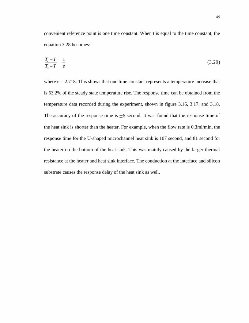
temperature data recorded during the experiment, shown in figure 3.16, 3.17, and 3.18.

The accuracy of the response time is second. It was found that the response time of

the heat sink is shorter than the heater. For example, when the flow rate is ml/min, the

response time for the U-shaped microchannel heat sink is 107 second, and 81 second for

the heater on the bottom of the heat sink. This was mainly caused by the larger thermal

resistance at the heater and heat sink interface. The conduction at the interface and silicon

substrate causes the response delay of the heat sink as well.

46

Figure 3.16. Response time vs. flow rate for low heat flux.

The response time has a decreasing trend with an increasing flow rate. The response time

t was 92 seconds for U-shaped channel when flow rate was 0.4 ml/min, and heat flux was

1286 W/m2 as shown in Figure 3.16, while it was 121 second and 110 second for straight

channel and serpentine channel, respectively. The U-shaped channel heat sink took a

shorter time to reach steady state, and it responded faster and removed heat faster than the

other two configurations. This is caused by the flow structure and the ratio of the surface

area between solid (silicon) and liquid (distilled water). The edge outside the arc area of

the U-shaped channel has large solid area compare with other configurations. The

serpentine channels had the lowest heat removal rate within the experimental range. The

47

difference in the response time between the straight channel heat sink and the serpentine

channel heat sink becomes shorter with increasing flow rate at the top surface of the heat

sink, even though they still took longer time to reach steady state condition compared to

the U-shaped channel.

Figure 3.17. Response time vs. flow rate for high heat flux.

Figure 3.17 shows the response time for different flow configurations, with different heat

flux but the same flow rate. The flow rate was fixed at 0.4ml/min, and response time

varies between 83 sec and 101 sec for a U-shaped channel when the heat flux is increased.

Straight channel and serpentine channels had longer response time, compare with U-

shaped channel. Overall, the influence of the heat flux to the response time is smaller

than the influence of the flow rate.

48

Figure 3.18. Response time vs. heat flux for different heat sinks.

49

Chapter 4 Numerical Simulation and Parametric Study of Microchannel Heat Sink

The purpose of this chapter is to build numerical models for the heat sink devices tested

in the experiment including the straight channel, bended channel, and Y-shaped channel.

The numerical models will be calibrated by the experimental results. The validated

numerical models will be used to extend the experimental analysis to include higher

aspect ratio channels and high Reynolds number flows. Effects of natural convection and

radiation, viscous dissipation, and axial heat conduction are discussed. The numerical

models are applied with constant pressure drop, constant pumping power and constant

volumetric flow and the results will be presented and discussed.

4.1 Numerical model construction

4.1.1 The effect of viscous dissipation

The viscous dissipation refers to converting energy from work done by shear force of the

liquid to heat. The coolant experiences a pressure drop due to friction as it flows

downstream. Assuming that the walls are adiabatic, the thermal energy converted from

the pressure drop will lead to the fluid temperature rise:

50

vh

p

PT

C

(4.1)

where is the pressure drop, is the temperature rise due to viscous heating, which

is independent of the heat flux applied on the walls. The effect of viscous heating can be

significant given a large pressure drop. However, the effect of viscous heating on

temperature is small for this study especially for the study range of the experiment. For

example, room temperature (20 ºC) DI water with a pressure drop of 100kP will only lead

to a temperature rise of 0.02 ºC. Hence, the effect of viscous dissipation on temperature

rise is neglected in this study.

4.1.2 The heat transport mechanism other than forced convection

The effect of radiation heat transfer is small for electronic chips with high heat

dissipation. The amount of heat removed by radiation can be calculated by the Stefan-

Boltzmann Law. Tsutomu Sato (1967) observed that the emissivity of silicon varied from

0.4 to 15 at various temperatures from 340 K to 1070 K. For our study, the temperature

of silicon is below 100 ºC. With a relatively low emissivity, the heat transferred by

radiation is a small portion compare with the overall heat dissipation, which can be up to

nowadays. Hence, radiation heat transfer is negligible for this study.

The free convection will become significant with high temperature gradient, large

characteristic length of dimensions, or low diffusivity. A dimensionless number,

Rayleigh number is used to characterize convection problems in heat transfer.

51

3Pr ( )x x s

gRa Gr T T x

(4.2)

Figure 4.1. Free, forced and mixed convection regimes for flow in horizontal tubes.

(Taken from Metais and Eckert).

Metais and Eckert recommended using figure 4.1 to identify the pure forced convection

or the mixed convection heat transfer regime. The shaded area is the transition region.

For any flow with given Reynolds number, the value of the parameter represents

whether it is necessary to consider buoyancy effects. In this study, if the velocity through

the microchannels is low enough, the free convection may have significant effect on the

heat transfer. One the other hand, if the Reynolds number is larger enough, and

52

is small enough, then the superimposed natural convection is not important. For example,

for room temperature water, the thermal expansion coefficient is about

, the density is , and kinematic viscosity ,

with the worst case scenario of ºC, the Rayleigh number is of order 1. This

suggests that the contribution of natural convection to the total heat transfer is small.

Hence, it is not accounted in the numerical model.

4.1.3 The physical model

It is computationally intensive to model the entire microchannel heat sink with 56 (for

straight and Y-shaped channel) or 28 microchannels (for U-shaped channel). Therefore,

simplified domains were used in this study. Figure 4.2 and figure 4.3 shows the

schematic computational domain of three different configurations of microchannel heat

sink devices tested in the experiment.

For the straight microchannel heat sink, because the entire heat sink is geometrical

symmetric, only half of the fin and half the microchannel are modeled as shown in figure

4.2(b). The left boundary and the right boundary are planes of symmetry. At the bottom

of the silicon substrate, a given constant heat flux q was imposed. In the experiment, the

top wall of the heat sink was covered with PDMS and its conductivity is three orders of

magnitude lower than that of silicon, it is assumed to be an adiabatic wall. The front (z=0)

and the back boundary (z=1cm) are velocity inlet and pressure outlet respectively.

53

(a) General configuration (b) Computational domain

Figure 4.2. Sketch of straight microchannel heat sink model.


Figure 4.3. Sketch of U-shaped microchannel heat sink model.

54

It is noted that for the U-shaped channel, the length of each channel is different. The

channel located at the center of the heat sink as shown in Figure 4.3(b) is chosen for our

study as the computational domain because there is very little spreading of the heat

towards the sides at the center. The computational domain for Y-shaped channel is shown

in Figure 4.4. For the first segment of the microchannel, half of one channel and half of

one fin with symmetric boundary condition were used. As the flow splits in the second

segment of the channel, two half channels with one fin in the middle were chosen as the

computational domain.


Figure 4.4. Sketch of Y-shaped microchannel heat sink model.

55

4.1.4 Mathematical formulation:

The mathematical formulation of the problem is described in this section. The numerical

method used for this study is also discussed here.

a) Governing equations:

The single phase liquid fluid behaves as continuum, incompressible, and laminar in the

presented study range, and there was no electrokinetic flow behavior. Therefore, the

conservation of mass, momentum and energy equations are applicable for solving the

steady state temperature and pressure:

Continuity equation:

0 V (4.3)

Navier-Stokes Equations:

2P V V g V (4.4)

Energy Equation:

2

pc T k T q V (4 .5 )

b) Boundary conditions:

In the 3D Cartesian Coordinate system shown in Figure 4.2 to Figure 4.4, at the entrance

of the heat sink assembly, uniformly distributed axial velocity and inlet temperature are

specified. Velocity along other two directions at the inlet is assumed to be zero. At the

exit for both configurations, pressure outlet boundary was used with zero gage pressure.

The top wall is assumed to be adiabatic. On the silicon substrate, all the wall surfaces are

56

assumed to be adiabatic. At the bottom of the substrate, a constant heat flux q is imposed.

The left boundary and the right boundary are symmetry boundaries.

The conjugate heat transfer is coupled with the fluid flow in the microchannels for this

problem. Hence, the governing equation (4.3) to (4.5), including the continuity,

momentum and energy equations are solved simultaneously. The finite volume method

(FVM) based on commercial software-ANSYS FLUENT with SIMPLE algorithm was

employed to solve the governing equations in the solid and fluid domains. The physical

models were meshed with regular structured grid of hexahedral mesh elements. The

QUICK scheme, which based on a weighted average of second order upwind and central

interpolations of the variable, will generate more accurate results on structured grids

aligned with the flow direction. Therefore, it was used to computing convective terms at

faces in this study. The grid dependence was tested. The linear set of equations is solved

with an implicit linear equation solver (Gauss-Seidel) in conjunction with an algebraic

multigrid method. The scaled residual of continuity was set to 10-6

and the residual of

energy was set to 10-8

magnitude as the convergence criterion.

4.1.5 Model validation

To validate the numerical model, the microchannel dimensions used in the experiment

are reproduced. The width of each microchannel is 100 µm, the height of the

microchannel is 175 µm, and the length of the channel is 1 cm, which is usually the same

as the length of the electronic chip.

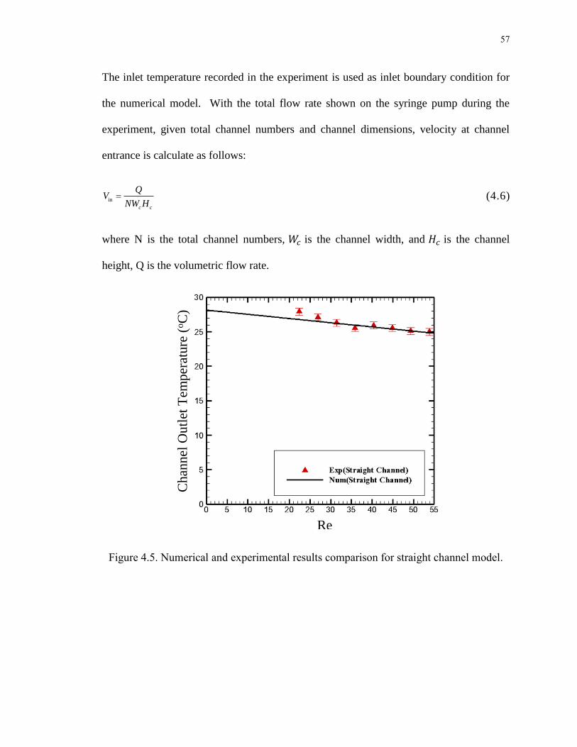
57

The inlet temperature recorded in the experiment is used as inlet boundary condition for

the numerical model. With the total flow rate shown on the syringe pump during the

experiment, given total channel numbers and channel dimensions, velocity at channel

entrance is calculate as follows:

in

c c

QV

NW H (4.6)

where N is the total channel numbers, is the channel width, and is the channel

height, Q is the volumetric flow rate.

Figure 4.5. Numerical and experimental results comparison for straight channel model.

Re

Ch

ann

el O

utl

et T

emp

erat

ure

(oC

)

58

Figure 4.6. Numerical and experimental results comparison for U-shaped channel model.

Figure 4.7. Numerical and experimental results comparison for Y-shaped channel model.

59

The comparison of current numerical study with experiment measured temperature

results at the exit of the channel are shown in figure 4.5, figure 4.6 and figure 4.7. The

agreement is very good and the difference is within 3.5% for straight channel model, and

2.2% for U-shaped channel model.

4.2 Parametric study for straight channel

The numerical model will be formulated for microchannels with different aspect ratios.

Different heat sink material and coolant material will be investigated. The numerical

models are also provided for different boundary conditions: constant heat flux, constant

pumping power, constant pressure drop, and constant flow rate. When one design

parameter is analyzed, all other design parameters will be held constant. The ‘baseline’

design is the water-cooled silicon heat sink, as described in the experiment. The thermal

and fluid performance of other designs will be compared with the ‘baseline’ case.

Three different aspect ratios corresponding to small, moderate and high

aspect ratio are included in the following figures. The channel height is , and

the channel width is . The corresponding substrate thickness is .

Note the single channel in the model is used to represent the thermal performance of the

heat sink with multiple channels. Hence, the total channel numbers are the same for heat

sinks with different aspect ratios. The channel hydraulic diameters are 200, 100, and

54.5 for the same channel height. The overall flow rate for the heat sink is 70 ml/min

for figure 4.7. The corresponding Reynolds numbers are: 92, 115, and 125, respectively.

60

The actual channel length is 1 cm. The dimensionless axial distance in the flow direction

is defined in equation 3.7. The thermal resistance is defined as:

s

T TA

Q q

(4.7)

where is the surface area over which heat flux occurs. The heat flux is assumed to

be uniform over . Note that the thermal resistance definition is different from equation

3.17. This definition makes it possible to formulate the thermal analysis for the entire

heat sink based on a single channel and fin. Also, it makes more sense to compare the

thermal performance of difference configurations based on this parameter.

The thermal resistance as a function of distance from upstream rises quickly as the aspect

ratio decreases with constant flow rate as shown is figure 4.8. The black line, which

represents high aspect ratio channel, has the lowest thermal resistance and shows a less

thermal resistance gradient among three cases. Since the fin height and the distance from

the channel center to the adjacent channel center are constant, the low thermal resistance

for high aspect ratio channel is due to the increase of coolant velocity related to the

decrease in the flow cross section area. The thermal resistance for is 50% larger

than .

61

Figure 4.8. Thermal resistance vs. length for different aspect ratio.

The thermal resistance for three different flow rates is shown in figure 4.9. Three cases

presented in this plot have identical geometry. The thermal resistance decreases as the

flow rate increases as expected. The slope of the curve gets more and more flat when the

flow rate becomes larger. When the flow rate is doubled from 70 ml/min to 140 ml/min,

the average thermal resistance is increased by 32%. But when the flow rate is increased

from 140 ml/min to 280 ml/min, the average thermal resistance is only increased 25%.

62

Figure 4.9. Thermal resistance vs axial distance for different flow rates ( ).

The fluid performance is evaluated by pumping power of the heat sink, which is defined

in equation 4.8:

avg cP Q p n u A p (4.8)

63

The pumping power corresponding to different aspect ratios is the starting points of the

curves shown in figure 4.10. It is increased exponentially as the aspect ratio increases.

The pumping power is 0.004W for , 0.053W for , and 0.389W for

Note that the pumping power is continuously increasing with the flow rate for different

aspect ratios, as shown in figure 4.10. The pumping power requirements for are

always larger.

Figure 4.10. Pumping power vs flow rate for cases with different aspect ratios.

The pressure drop is represented by a dimensionless term-- Euler Number. Euler number

is defined as:

64

2 2app

hm

P LEu f

Du

(4.9)

Figure 4.11. Euler number vs. Reynolds number for different aspect ratios.

With constant properties and fixed channel dimensions, Euler number essentially

provides the same information as the fanning friction factor . In laminar flow

region as show in figure 4.11, the Euler number, which is corresponding to a smaller

friction factor, keeps decreasing when Reynolds number is increased, but the

decreasing rate is dropping. Better thermal performance is reached with high Reynolds

number for laminar flow as shown in figure 4.12. The trade-off of reducing the friction

65

factor as well as thermal resistance is the large pumping power and low energy

efficiency.

Figure 4.12. Thermal resistances vs. Reynolds number for different aspect ratios.

Figure 4.13 presents the thermal and fluid performance results for comparison of constant

pressure drop. Note that the thermal resistance for constant pressure drop constraint

behaves similar for and , though the pumping power of the latter is 3.85 time

larger. When the aspect ratio is 10, the thermal resistance is the highest, with a low

pumping power requirement (0.16 W).

66

Table 4.1. Temperature vs. aspect ratio for different heat fluxes.

Heat Flux ( ) Temperature (ºC)

100 30.43 33.76 43.26

200 40.86 47.51 66.6

400 71.72 75.02 113.06

Thermal resistance 0.1 0.14 0.23

Figure 4.13. Thermal resistances vs. axial distance for constant pumping power.

The average temperature on the bottom of the channel for various heat fluxes is shown in

table 4.1 (The pumping power requirements remain the same for the same aspect ratio).

67

The average thermal resistance of the heat sink with the same aspect ratio is shown in the

last row. The purpose of this comparison is to show that the thermal performance of

remains the same as the heat flux increases.

Figure 4.14. Thermal resistances for different coolants at constant flow rate.

Figure 4.14 and figure 4.15 present the thermal resistance for a comparison of various

liquid coolants at constant flow rate and constant pressure drop, respectively. The

corresponding pumping power of four different coolants is list in table 4.2. DI water

68

provides the best thermal performance. Methanol/water, which shows the second best

performance, is a low cost antifreeze solution finding use in refrigeration services and

ground source heat pumps. The major disadvantages of methanol are toxicological and

flammable. FC-77 is preferable to water in certain circumstance to avoid contamination

and corrosion of the chip when the coolant is in direct contact with the IC chip. Mercury

are less practical, though recently, liquid metal has been utilized with

magnetofluiddynamic(MFD) pump to remove high heat flux from microprocessors.

Figure 4.15. Thermal resistances for different coolants at constant pressure drop.

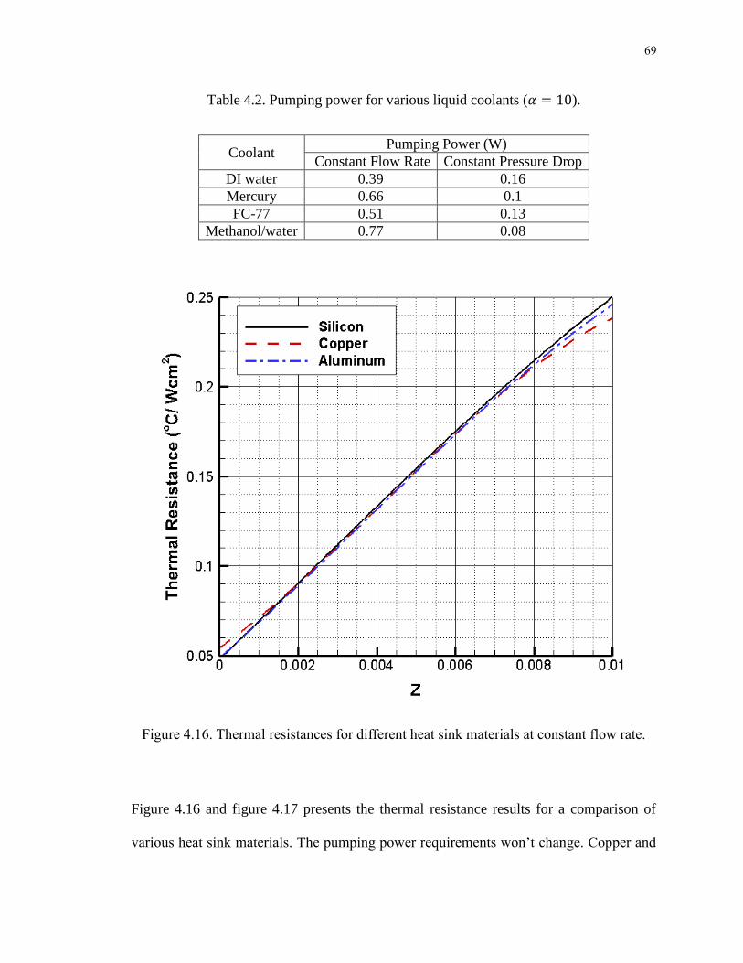
69

Table 4.2. Pumping power for various liquid coolants ( ).

Coolant Pumping Power (W)

Constant Flow Rate Constant Pressure Drop

DI water 0.39 0.16

Mercury 0.66 0.1

FC-77 0.51 0.13

Methanol/water 0.77 0.08

Figure 4.16. Thermal resistances for different heat sink materials at constant flow rate.

Figure 4.16 and figure 4.17 presents the thermal resistance results for a comparison of

various heat sink materials. The pumping power requirements won’t change. Copper and

70

aluminum provide slightly smaller thermal resistance due to the higher thermal

conductivity compare to silicon, but not significantly. If the copper or aluminum will be

used as the heat sink material, an interface will be required instead of directly fabricated

on back of the electronic chip. Therefore, an extra interface thermal resistance will be

generated and influence the overall thermal performance.

Figure 4.17. Thermal resistances for different heat sink materials at constant pressure

drop.

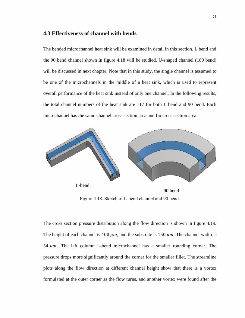
71

4.3 Effectiveness of channel with bends

The bended microchannel heat sink will be examined in detail in this section. L bend and

the 90 bend channel shown in figure 4.18 will be studied. U-shaped channel (180 bend)

will be discussed in next chapter. Note that in this study, the single channel is assumed to

be one of the microchannels in the middle of a heat sink, which is used to represent

overall performance of the heat sink instead of only one channel. In the following results,

the total channel numbers of the heat sink are 117 for both L bend and 90 bend. Each

microchannel has the same channel cross section area and fin cross section area.

L-bend

90 bend

Figure 4.18. Sketch of L-bend channel and 90 bend.

The cross section pressure distribution along the flow direction is shown in figure 4.19.

The height of each channel is , and the substrate is . The channel width is

54 . The left column L-bend microchannel has a smaller rounding corner. The

pressure drops more significantly around the corner for the smaller fillet. The streamline

plots along the flow direction at different channel height show that there is a vortex

formulated at the outer corner as the flow turns, and another vortex were found after the

72

flow changes directions. This is adverse to heat transfer and may cause the local

temperature increase at the corner. A large fillet helps to reduce the local flow circulation

as shown on the right column in figure 4.19. For the 90 bend, there is no sharp corner

hence the flow turns smoothly.

(a) Cross Section Pressure Drop

(b) Cross Section Pressure Drop

fillet

fillet

fillet

Figure 4.19. Normalized pressure and streamlines for L bend with different fillets.

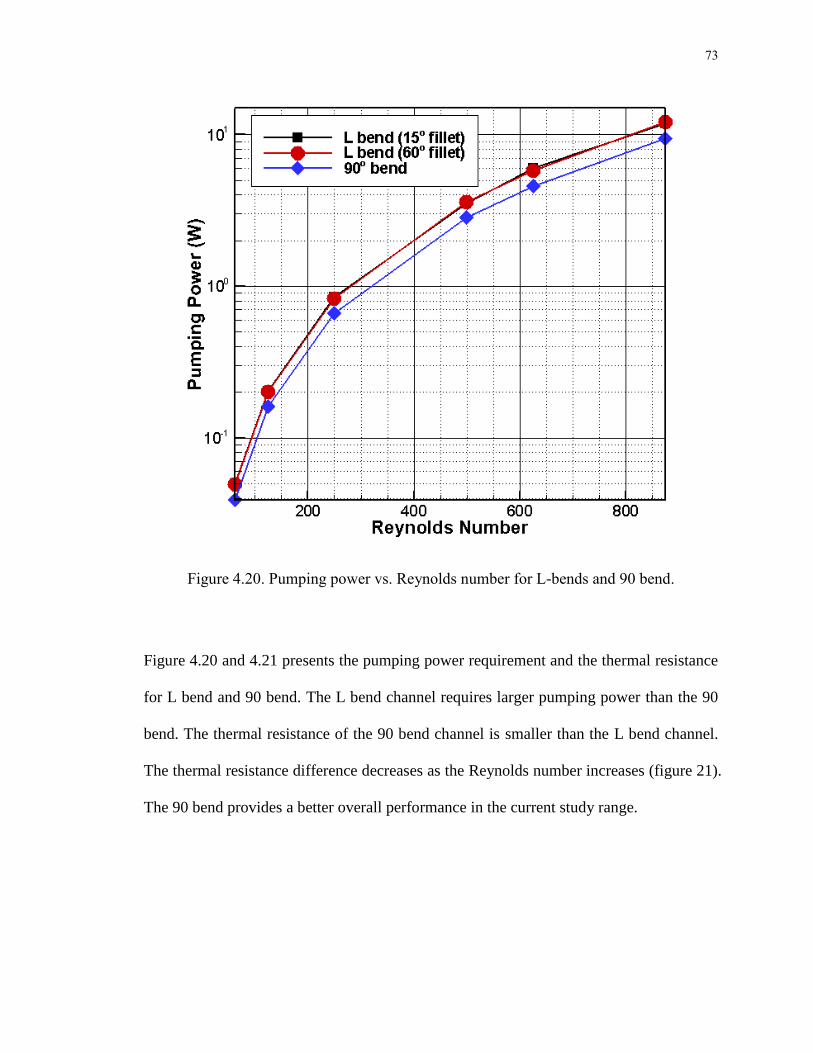
73

Figure 4.20. Pumping power vs. Reynolds number for L-bends and 90 bend.

Figure 4.20 and 4.21 presents the pumping power requirement and the thermal resistance

for L bend and 90 bend. The L bend channel requires larger pumping power than the 90

bend. The thermal resistance of the 90 bend channel is smaller than the L bend channel.

The thermal resistance difference decreases as the Reynolds number increases (figure 21).

The 90 bend provides a better overall performance in the current study range.

74

Figure 4.21. Thermal resistance vs. Reynolds number for L-bends and 90 bend.

4.4 Effectiveness of channels with branches (Y-shaped channels)

Given the same inlet coolant velocity, the thermal performance in a channel with fined

structure will be enhanced when the flow is not fully developed. In this study, the second

segment of the channel structure allows the fluid departure from the fully developed flow

from the first segment.

75

Figure 4.22 shows the temperature distribution at y= 10, 75, and 160 in the channel,

assuming the heat flux ̇ generated by the electronic chip is 200 , and the flow

rate is 150 ml/min. the temperature is higher on the bottom of the channel, and it is more

evenly distributed as y increases. It is noted that along the flow direction, the highest

temperature happened in the first segment of the device, before the flow splitting into two

different channels. It is different from the continuous straight channel, which usually has

the highest temperature show at the exit of the channel.

(a) Y-shaped channel sketch (b) Temperature distribution

Figure 4.22. Temperature distribution in Y-shaped channel.

Figure 4.23 gives the velocity distribution along z direction when y is75μm. The velocity

reaches the maximum value after the channel pattern changed. The high velocity speed

and the remixing at the entrance of the second segment of the channel causes the

increasing of the heat transfer rate.

76

Figure 4.23. Velocity distribution in Y-shaped channel (along the flow direction).

An increase of flow rate appears to be necessary to increase the heat transfer coefficient.

The high inlet velocity will increase the pressure drop at the same time. For the same

channel length and hydraulic diameter, the pressure drop with inlet Reynolds number

1038 is increased by 77% than the pressure drop at Reynolds number 346, which

corresponds to a three times larger flow rate. For low Reynolds number (Re=346), the

flow is disturbed but smoothly redirected, so no vortices was created. The flow tends to

gathered gradually from the top and bottom of the side walls to the center as shown on

the left in Figure 4.24. High Reynolds number will tend to create transverse vortices. For

example, when Re is 1038 in this study, two pairs of vortices were generated closer to the

fin shown on the right in Figure 4.24. The vortices happened at the cross section area

allow for transverse coolant mixing, which spreads out the downstream high coolant

temperatures from high heat dissipation zones. They also draw more coolant to the hot-

spots since the coolant viscosity is lower at high temperature region.

77

Figure 4.24. Transverse streamlines for different Re number.

The bifurcation microchannel heat sink (Y-shaped channel) provide potential advantages

if design properly. Design and optimization of other geometry parameters, such as the

total channel numbers, microchannel width, and height will be discussed for heat sink

with continuous straight channel in chapter 5. The same approach and parameters can be

used to study the heat sink bifurcation channels. In this section, the thermal and fluid

78

performance prediction for various channel length ratios is presented. Figure 2.25 shows

the average thermal resistance versus α, which is defined as:

1L

L (4.10)

is the channel length of the first segment, with the channel width and channel

height . L is the total length of the heat sink, which is fixed as 1 cm in this study.

Figure 4.25. Thermal resistance and non-dimensional pressure drop vs. different channel

length for Y-shaped channel

79

The corresponding non-dimensional pressure drop is also shown in Figure 4.25. For a

given flow rate (150 ml/min for figure 4.25), having the flow splitting into two branches

will change average thermal resistance. When L1 is 0.2 cm, the thermal resistance was

increased by 5%, and the pressure drop was also increased by 14%. There are several

factors which account for this degradation of the thermal performance. For example, the

Reynolds number is too low to allow vortex generation and unsteady flow to occur as

shown in figure 4.24. The ratio of the fin thickness to the fin length may have been too

low. As the channel length of the first segment kept increasing, the thermal resistance

will increase but the pressure drop will decrease.

80

Chapter 5 Design and Optimization of Microchannel Heat Sinks

The purpose of this chapter is to utilize numerical models built for the heat sink devices

in the previous chapter to discuss the design and optimization of multi-microchannel heat

sink systems. The parametric modeling techniques will be reviewed in this chapter, based

on which the optimization problem will be formulated. Two different configurations of

multiple microchannel heat sinks, straight and U-shaped channel designs with liquid flow

are investigated for electronic chip cooling. Three responses including thermal resistance,

pressure drop, and maximum temperature are parametrically modeled with respect to

various design variables including dimensions of channels, total channel numbers, and

flow rates. The multi-objective optimization problems, which minimize the thermal

resistances and pressure drops simultaneously, are formulated and studied. Some physical

constraints in terms of channel height, maximum temperature, and pressure are further

investigated. The Pareto frontiers are studied and the trade-off behaviors between the

thermal resistances and pressure drops are discussed.

5.1 Formulation of the design problem

The formulation of the design problem is a very important aspect in design and in other

engineering activities. The design process depends on the problem statement and so does

the evaluation of the design. Therefore, once the requirements of the system are decided,

the design obtained must meet all the requirements, and satisfy all the constraints and

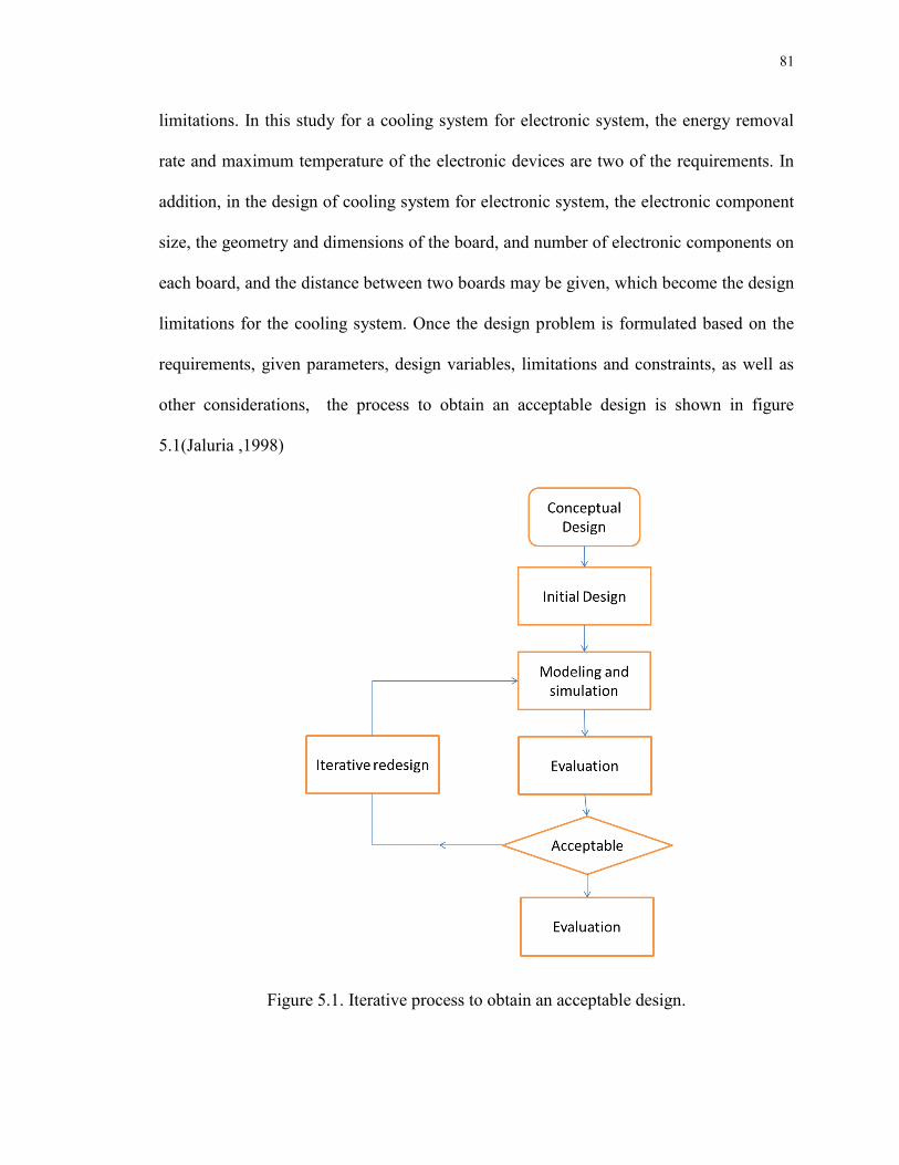
81

limitations. In this study for a cooling system for electronic system, the energy removal

rate and maximum temperature of the electronic devices are two of the requirements. In

addition, in the design of cooling system for electronic system, the electronic component

size, the geometry and dimensions of the board, and number of electronic components on

each board, and the distance between two boards may be given, which become the design

limitations for the cooling system. Once the design problem is formulated based on the

requirements, given parameters, design variables, limitations and constraints, as well as

other considerations, the process to obtain an acceptable design is shown in figure

5.1(Jaluria ,1998)

Figure 5.1. Iterative process to obtain an acceptable design.

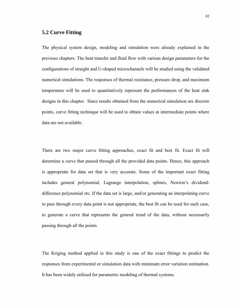
82

5.2 Curve Fitting

The physical system design, modeling and simulation were already explained in the

previous chapters. The heat transfer and fluid flow with various design parameters for the

configurations of straight and U-shaped microchannels will be studied using the validated

numerical simulations. The responses of thermal resistance, pressure drop, and maximum

temperature will be used to quantitatively represent the performances of the heat sink

designs in this chapter. Since results obtained from the numerical simulation are discrete

points, curve fitting technique will be used to obtain values at intermediate points where

data are not available.

There are two major curve fitting approaches, exact fit and best fit. Exact fit will

determine a curve that passed through all the provided data points. Hence, this approach

is appropriate for data set that is very accurate. Some of the important exact fitting

includes general polynomial, Lagrange interpolation, splines, Newton’s dividend-

difference polynomial etc. If the data set is large, and/or generating an interpolating curve

to pass through every data point is not appropriate, the best fit can be used for such case,

to generate a curve that represents the general trend of the data, without necessarily

passing through all the points.

The Kriging method applied in this study is one of the exact fittings to predict the

responses from experimental or simulation data with minimum error variation estimation.

It has been widely utilized for parametric modeling of thermal systems.

83

The covariance vector which contains M components of the covariance functions is given

by:

1

( , ) Cov ,M

S S

x j j

j

C x x

x x e (5.1)

The approximation function F is defined by the dot product between the coefficient

vector w and the covariance vector :

( , )S

xF C x x x w (5.2)

where x is the design variable; is the 𝑗 sampling point; M is the number of sampling

points; je is the thj normal basis; the notation of dot product is used for the scalar

product, the tensor operating on a vector, and the product of tensors.

For each sampling point S

jx , the response S S

j jF x is expressed by

S

j j k k nm m n mn m n k kF w C C w e e e e e e e (5.3)

which is written in the Einstein summation convention. In Equation 6.3, the component

of the covariance tensor C is defined as Cov ,S S

mn m nC x x and TC C is given. Therefore,

the coefficient vector w can be determined by

1

1 1, , , ,S S S S S

M M

w C x x F x x (5.4)

84

where S S

j jFF e . Common Covariance Functions for different Kriging Techniques

including Gaussion covariance function, Pseudo-cubic spline, Radial basis function, and

etc. In this study, the exponential covariance function is considered:

Cov , 1 exp ,m n m n x x x x (5.5)

It is noted that there is no approximation error at the sampling points; however, the

approximations near the boundaries of design of experiments are less accurate than the

interior part. The interior sampling spaces are chosen to be the design spaces for the

parametric models in this section and the optimization processes in the next section.

5.3 Straight Channel Model

In the design of straight microchannels, various parameters affect the heat transfer

performances, including the experimental parameters of fluid flows and the geometries of

heat sinks. In order to simplify the complicated models of microchannel thermal

systems, the flow rate 3 -1(m s )Q and three geometrical parameters are considered while

other parameters are fixed. The first geometrical variable is the dimensionless height H ,

which is given by

c c sH H H H (5.6)

where c sH H equals the wafer thickness, 550 μm . The second one is the dimensionless

width W which is defined as

c c fW W W W (5.7)

85

And the last one is the number of microchannels N . The denominator in Equation 6.7

remains constant when N is fixed.

The validated model shares the same dimension with the experimental device, which

corresponding to 56 channel numbers. Instead of modeling with respect to the four

design variables, the responses are first parametrically modeled with respect to and

as baseline models considering constant . Five uniformly distributed sampling

points are considered for each design variable, listed in Table 5.1, and only

simulations are needed. Next, the effects of channel number are studied while

fixing the channel height. In our experiment settings, the thickness of photoresist 1518

for the plasma etching of microchannels in the silicon wafer is limited to≤ ;

accordingly, the maximum height of microchannel is around 400 . Therefore, the

responses are also modeled with respect to under the consideration of

. Due to the scaling effects in the channel numbers, the five integer points

are uniformly sampled in the logarithm of , listed in Table 5.1, and further

simulations are considered. The sampling space of is chosen to ensure the

channel hydraulic diameter ranges from 10 to 200 ; following Kandlikar (2003)’s

classification of microchannels

For each numerical simulation, three significant responses are studied. Two quantitative

measures, including thermal resistance and pressure drop , to represent the thermal

performances are chosen as the first two responses. The lower the first two responses are,

86

the higher the efficiency is and the lower the pumping power requirement is. Since the

existence of any hot spot will decrease the reliability of the electronic chip, the maximum

temperature is considered as the third response and monitored to avoid

malfunctions.

Table 5.1. Sampling points for straight channel model.

Sampling points 1 2 3 4 5

6 3 -1( 10 m s )Q 1.17 1.33 1.50 1.67 1.83

H 100/550 200/550 300/550 400/550 500/550

W 1/6 1/3 1/2 2/3 5/6

N 56 97 167 289 500

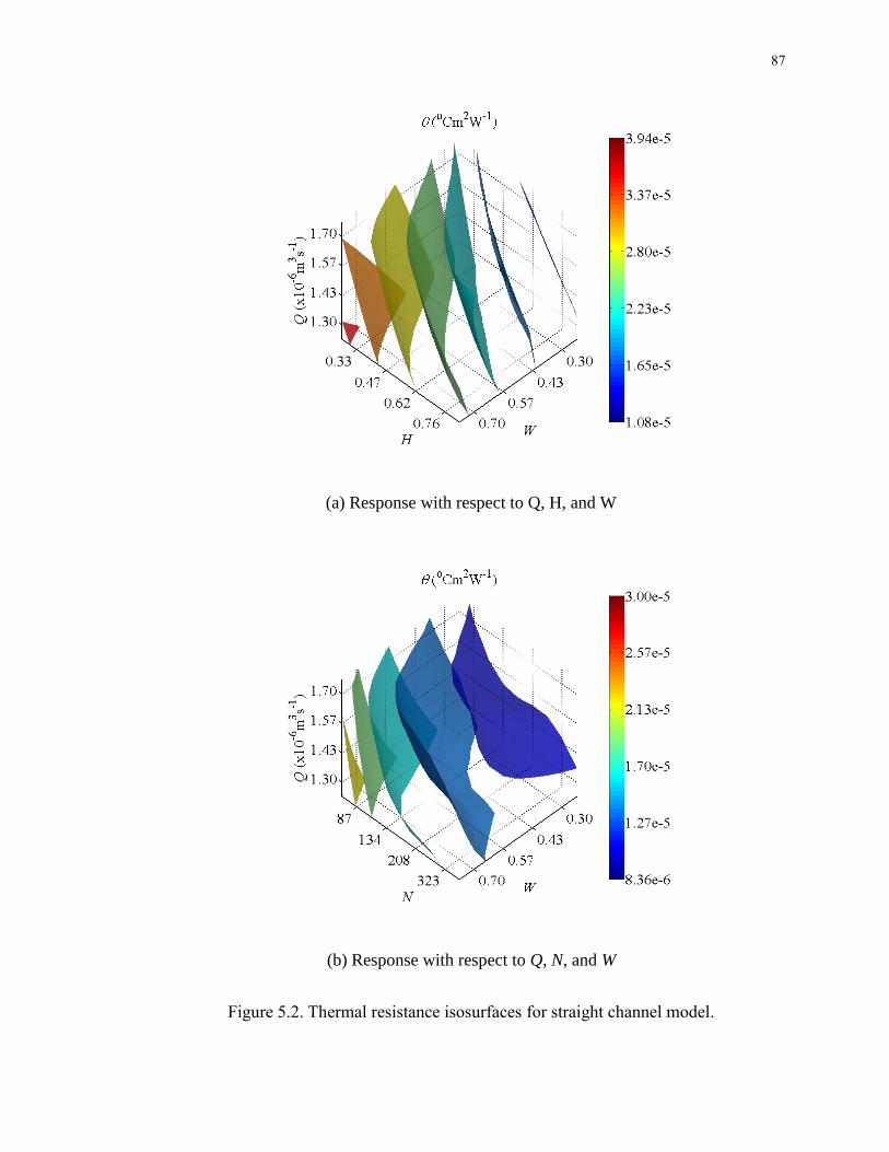
87

(a) Response with respect to Q, H, and W

(b) Response with respect to Q, N, and W

Figure 5.2. Thermal resistance isosurfaces for straight channel model.

88

The first response, thermal resistance , is calculated using the heat flux as the current

and 𝑔 − 𝑛 as the potential:

avg inT T q (5.8)

where 𝑔 is the average temperature of the heating area; 𝑛 is the inlet coolant

temperature; remains constant. The response isosurfaces of are

shown in Figure 5.2. The isosurface (a) is formulated under the constant while

varies from 1.08 to 3.94 510 . In the given sampling space, monotonically

decreases when and increase and decreases. The isosurface (b) considers constant

. As a result, decreases as increases because of the increment of the

total surface area for heat transfer.

The second response, pressure drop , is parametrically modeled with respect to the

previously described variables. Figure 5.3(a) shows the isosurface of with respect to

, , and while the subfigure (b) presents the one with respect to , , and . The

colorbars are presented in the scale of logarithm of due to the wide range of

responses in the sampling spaces. It is as expected that the pressure drop between the

inlet and outlet of fluid decreases when the velocity decreases. The pressure drop

decreases when and increases; on the other hand, is smaller when decreases

because of the resultant decrement of inlet velocity. It is noted that the physical

behaviors of and both decrease with higher but conflict with each other

associated with Hence, the trade-off between and is studied in the

formulations of the multi-objective optimization problems in the next section.

89



Figure 5.3. Pressure drop isosurfaces for straight channel model.

Alternative View

90


(b)Response with respect to Q, N, and W

Figure 5.4. Maximum temperature isosurfaces for straight channel.

91

Lastly, the third response, the maximum temperature , is shown in Figure 5.4. The

behaviors of are similar to the thermal resistance: is inversely proportional to

but positively proportional to . The responses of represent the average

performances of the microchannel heat sink designs while the responses of provide

the extreme thermal behaviors of the designs. The measure of is important because

it cannot exceed the allowable level and the hot spots can be avoided. In the next section,

the constraints associated with the maximum temperatures are also studied in the

optimization formulations.

5.4 U-shape channel model

The second configuration is the U-shaped microchannel design. Similar to the straight

microchannel design, the three responses for the U-shaped designs are first parametrically

modeled with respect to considering constant , which is one half of

the straight channel number, requiring 125 simulations. The U-shaped microchannel

design with can be compared with the straight design with because their

total surface areas are the same and the channels of inlet and outlet cross sections are

identical at the front sides. The sampling points in for the U-shaped designs,

listed in Table 5.2, follow the straight designs; accordingly, the Re varies from 127 to

1003 and the flow remains laminar. Furthermore, the responses are modeled with respect

to with the considerations of constant , which needs 100 more

simulations. The five uniformly sampling points in the logarithm of N are also listed in

table 5.2.

92

The thermal resistances, shown in figure 5.5, behave differently compared with the

straight designs. The measures of are very nonlinear with respect to while the trends

against are similar. The maximum thermal resistance of the U-shaped

channel design, 5 m in subfigure (a), is lower than the straight

channel designs: 5 in figure 5.2 (a); however, the minimum

measure, 5 in Figure 5.5 (a), is higher than the straight designs:

5 in Figure 5.2 (a). For U-shaped designs, the flow directions at the

curved areas are changed resulting in the formations of flow circulations, which provide

better mixing of fluid and enhance heat transfer, but leading to backflows, which are not

favorable for cooling. The overall performances of the U-shaped channel designs depend

on the dominance of the aspects of circulations and backflows. Similar behaviors can be

found in the responses of thermal resistances with respect to

Table 5.2. Sampling points for U-shaped channel model.

Sampling points 1 2 3 4 5

6 3 -1( 10 m s )Q 1.17 1.33 1.50 1.67 1.83

H 100/550 200/550 300/550 400/550 500/550

W 1/6 1/3 1/2 2/3 5/6

N 28 48 84 145 250

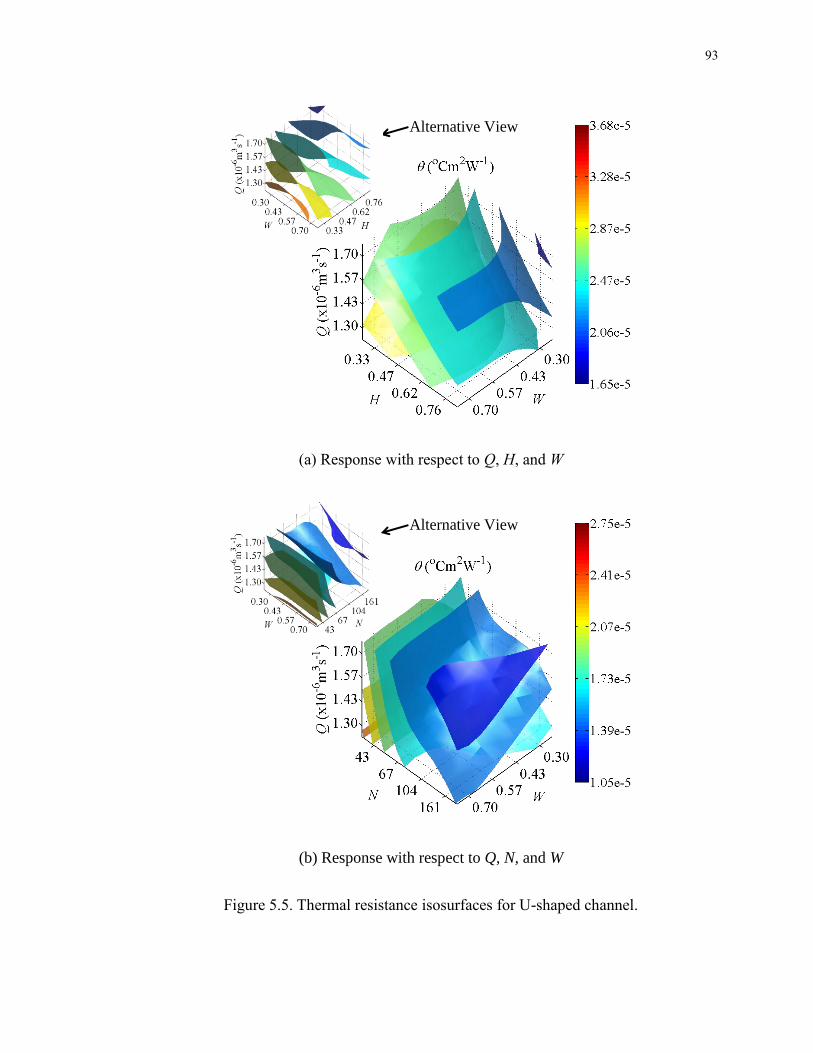
93



Figure 5.5. Thermal resistance isosurfaces for U-shaped channel.

Alternative View

Alternative View

94

The pressure drops for the U-shaped channel models are shown in Figure 5.6. The

alternative views are used for better visualizations of the isosurfaces while the colorbars

are used in the scale of double logarithms of . In the U-shaped designs, the trade-off

of enhancement of the thermal resistance is the increment of the pressure drop. Though

the trends of pressure drops in the U-shaped designs are similar to the straight designs,

the maximum in Figure 5.6(a), is higher than the straight design in

Figure 5.3 (a), ; furthermore, the maximum in Figure 5.6 (b),

8 , is further greater than the one in Figure 5.3 (b), 7 . The additional

pressure drop for the U-shaped channel is primarily the result of secondary flow which is

happened at the bended area.

Lastly, the responses of maximum temperatures, shown in Figure 5.7, are nonlinear

associated with . Furthermore, the maximum in the subfigure (a) is around 10ºC

higher than the straight channel design in Fig.5.4 (a). Therefore, it is important to find

the optimal designs which have allowable maximum temperatures to avoid the

malfunctions of the electronic devices.

95



Figure 5.6. Pressure drop isosurfaces for U-shaped channel.

Alternative View

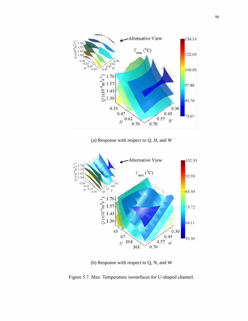
96



Figure 5.7. Max. Temperature isosurfaces for U-shaped channel.

Alternative View

97

5.5 Optimization problems

In this section, the response surfaces presented previously are used to formulate the

optimization problems for both the straight and U-shaped microchannel heat sink designs.

In order to get a better thermal performance with a reasonable pumping power

requirement, the thermal resistance and pressure drop should be minimized

simultaneously. The multi-objective optimization formulations are presented as well as

the effects of physical constraints.

5.5.1 Example 1 for straight channel model

The first example is a multi-objective formulation using the weighted-sum method (Deb,

2001):

, ,

6 3 -1

, , 1 , ,

. . 1.23 1.77 ( 10 m s )

0.25 0.84

0.23 0.77

0 1

Q H WMin w Q H W w P Q H W

s t Q

H

W

w

( 5 . 9 )

where the thermal resistance and pressure drop, shown in Figures 5.2(a) and 5.3 (a)

respectively, are minimized simultaneously with respect to considering

constant . The design variables are bounded in the intervals chosen from the

interiors of the sampling spaces. The optimization problem listed in equation 5.9 is

solved by the optimization toolbox in Matlab® with various weighting parameters, i.e.

. The optimal solutions vary with respect to and the

trade-off behavior between both objectives is presented by the Pareto frontier in Figure

5.8. The Pareto frontier not only provides a set of optimal solutions which satisfy the

98

multi-objective problem in equation 5.9 but also offers more flexibility for design

engineers than single-objective formulations.

When , the optimal solution is found at [ ] [ ]

and the minimum pressure drop is obtained; furthermore, the thermal

resistance is 5 . On the other hand, the minimum thermal

resistance 5 but higher pressure drop 5

are found when ; accordingly, the optimal reaches the upper bound

and is found at the lower bound 0.23. For each value of , is found at the

upper bound 0.84 indicating that maximum channel height provides the best heat transfer

performance.

The problem listed in equation 5.9 is furthermore studied with the considerations of the

following physical constraints:

o

1

5

2

3

: , , 90 ( C)

: , , 2.1 10 (Pa)

: , , 400 (μm)

m

c

g T Q H W

g P Q H W

g H Q H W

(5.10)

First of all, the maximum temperature, shown in Figure 5.4 (a), is controlled under 90 C

to prevent the malfunction of the electronic chips. According the performance curve of

Parker miniature diaphragm pump (Data Sheet of Miniature Diaphragm Pumps from

Parker Hannifin Corp), the pressure drop cannot exceed 5 in order to deliver

the flow rate and keep the pumping power in the acceptable ranges. As noted previously,

99

the channel height cannot be larger than due to the fabrication limitations. The

Pareto frontier under the constraints equation 5.10 is also shown in Figure 5.8.

The physical constraints narrow the design spaces and the optimal solutions are found on

the active constraint for each value of . Instead of reaching the upper limit of H in

the unconstrained problem (Equation 5.9), the optimal is found on the third

constraint; therefore, the constant is considered in the next optimization

problem with respect to . Furthermore, more conservative designs with higher

thermal resistances and pressures drops are found when considering the physical

constraints (Equation 5.10). For example, the optimal objectives are [ ] [

5 ] for and equal [ 5 5] for . More detailed

information about the optimal solutions is listed in table 5.3.

Figure 5.8. Pareto frontiers of example 1.

100

5.5.2 Example 2 for straight channel model

The second example first presents the unconstrained multi-objective problem

investigating the effects of channel numbers:

, ,

6 3 -1

, , 1 , ,

. . 1.23 1.77 ( 10 m s )

70 402

0.23 0.77

0 1

Q N WMin w Q N W w P Q N W

s t Q

N

W

w

(5.11)

which considers constant . The thermal resistance and pressure drop, shown in

Figures 5.2 (b) and 5.3 (b) respectively, are minimized simultaneously following the

optimization settings in Example 1. Furthermore, the optimization problem considering

the following physical constraints is investigated.

o

1

5

2

: , , 90 ( C)

: , , 2.1 10 (Pa)

mg T Q N W

g P Q N W

(5 .12 )

The Pareto frontiers for the unconstrained and constrained problems are shown in Figure

5.9.

As a result, the optimal solutions for both cases are identical when ≤ ≤ . For

≥ , the solutions [ ] [ ] reach the limit state of

2g for the constrained problems and the objectives are [ ] [

5 5]. On the other hand, is as low as at for the

unconstrained formulation; in this case, the channel number reaches the upper limit, i.e.

101

. It is as expected that maximum channel number produces largest surface area

for heat transfer resulting lowest thermal resistance; however, the highest pressure drop

is found. More detailed information about the optimal solutions is listed

in Table 5.4


5.5.3 Example 3 for U-shape channel model

For the U-shaped microchannel heat sink designs, the multi-objective formulations

follow the Equation 5.9 and physical constraints in Equation 5.10 are also studied. The

optimization settings follow the Example 1. The Pareto frontiers for both unconstrained

and constrained formulations are shown in Figure 5.10. The detailed information of the

optimal solutions is given in Table 5.5. Similar to Example 1, the design spaces become

smaller and more conservative designs are found when physical constraints are

102

considered. For both constrained and unconstrained formulations, the optimal thermal

resistances of the U-shaped designs, enhanced by the circulations of fluids in the curved

geometries of microchannels, are lower than the straight designs when .

However, both the thermal resistances and pressures drops in the U-shaped designs are

relatively higher than the straight designs in the other cases.


5.5.4 Example 4 for U-shaped Channel model

In order to study the effects of channel numbers, the multi-objective formulations in

equation 5.11 with and without the physical constraints (equation 5.12) are investigated

while is bounded by [35, 201] for the U-shaped designs. Following the same

optimization settings, the resultant Pareto frontiers and optimal solutions are shown in

Figure 5.11 and Table 5.6 respectively. In the cases of ≤ ≤ , identical results

103

are found for both unconstrained and constrained problems; otherwise, more conservative

designs are found in the constrained formulations. Compared with the straight

microchannel designs, lower thermal resistances in the U-shaped designs are found at

≤ for both unconstrained and constrained formulations. Furthermore, the pressure

drops in U-shaped designs are lower than straight designs when ≥ for

unconstrained formulations and ≥ for constrained ones. The optimal results

presented in this paper provide a comprehensive guideline for the selections of the

geometries of microchannels, the experimental parameters, and the weighting coefficients

in the optimization formulations.


Two different configurations of multiple microchannel heat sinks, including the straight

and U-shaped channel designs, have been studied. The models have been designed with

104

respect to the experimental and geometrical parameters and studied by the numerical

simulations. The simulation data have been validated by comparing with the experimental

results. Various responses to represent the influences of flow rates and geometrical

variables to the heat transfer performances have been parametrically modeled and studied.

For both straight and U-shaped microchannel designs, the optimization problems have

been formulated to minimize the thermal resistances and pressure drops simultaneously.

The Pareto frontiers have been found and presented to demonstrate the trade-off

behaviors between the multiple objective functions. Furthermore, the optimization

problems have been studied with the considerations of the physical constraints. In the

constrained formulations, the feasible design spaces were narrowed and more

conservative optimal solutions have been found.

Table 5.3. Optimal solutions in example 1.

w

Unconstrained

[ ] [ ]

0 [ ] [ 5 ]

0.25 [ ] [ 5 ]

0.5 [ ] [ 5 ]

0.75 [ ] [ 5 ]

1 [ ] [ 5 5]

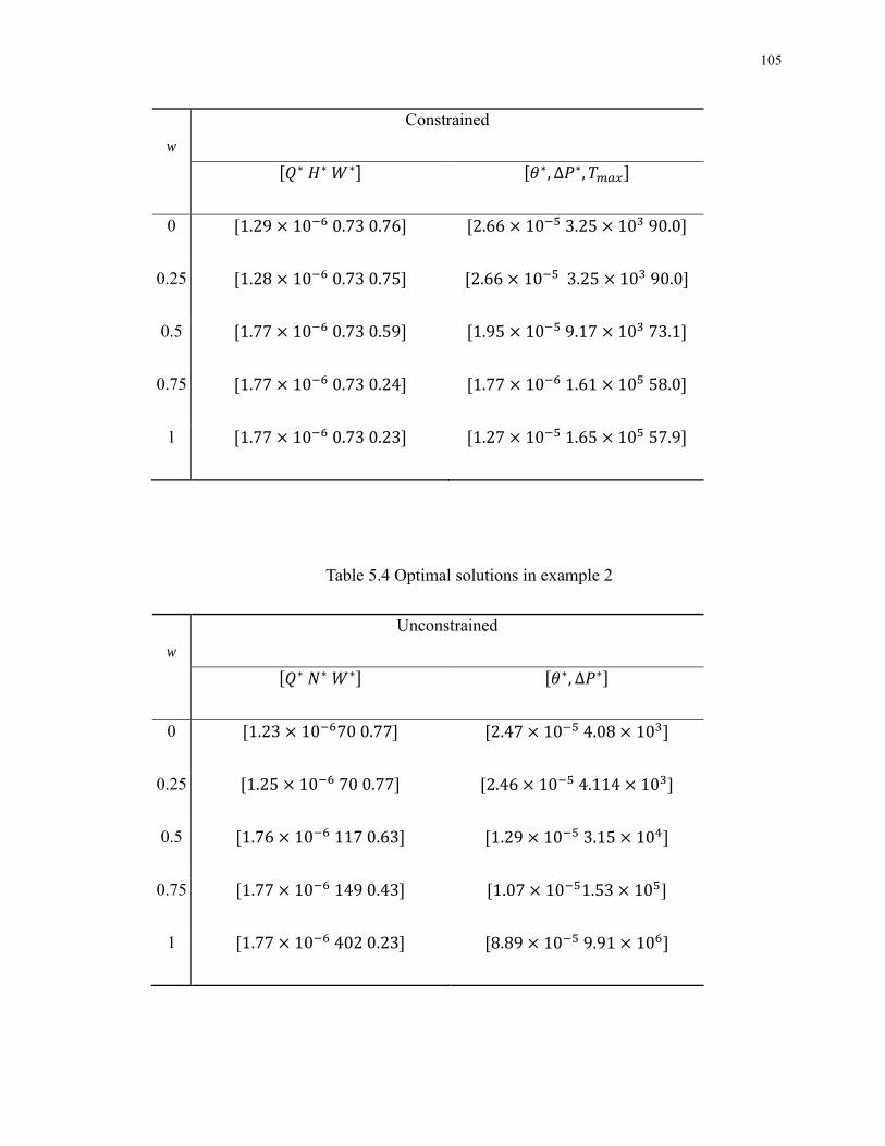
105

w

Constrained

[ ] [ ]

0 [ ] [ 5 ]

0.25 [ ] [ 5 ]

0.5 [ ] [ 5 ]

0.75 [ ] [ 5 ]

1 [ ] [ 5 5 ]

Table 5.4 Optimal solutions in example 2

w

Unconstrained

[ ] [ ]

0 [ ] [ 5 ]

0.25 [ ] [ 5 ]

0.5 [ ] [ 5 ]

0.75 [ ] [ 5 5]

1 [ ] [ 5 ]

106

w

Constrained

[ ] [ ]

0 [ ] [ 5 ]

0.25 [ ] [ 5 ]

0.5 [ ] [ 5 ]

0.75 [ ] [ 5 5 ]

1 [ ] [ 5 5 ]


w

Unconstrained

[ ] [ ]

0 [ ] [ 5 ]

0.25 [ ] [ 5 ]

0.5 [ ] [ 5 ]

0.75 [ ] [ 5 ]

1 [ ] [ 5 5]

107

w

Constrained

[ ] [ ]

0 [ ] [ 5 ]

0.25 [ ] [ 5 ]

0.5 [ ] [ 5 ]

0.75 [ [ ]

1 [ [ 5 5 ]


w

Unconstrained

[ ] [ ]

0 [ ] [ 5 ]

0.25 [ ] [ 5 ]

0.5 [ ] [ 5 ]

0.75 [ ] [ 5 5]

1 [ ] [ 5 ]

108

w

Constrained

[ ] [ ]

0 [ ] [ 5 ]

0.25 [ ] [ 5 ]

0.5 [ ] [ 5 ]

0.75 [ ] [ 5 5

1 [ ] [ 5 5 ]

It has been shown that the optimal experimental and geometrical parameters for the

minimum thermal resistances and pressure drops vary with respect to the preferences

from the designers. The detailed investigations presented in this paper not only provide a

comprehensive understanding of the influences of the design variables to the heat transfer

performances in both the straight and U-shaped microchannel models but also offer a

useful guideline for the selections of design parameters in the heat sink designs.

Furthermore, the developed strategies are useful for not only understanding the

fundamental heat transfer and fluid flow characteristics in the multiple microchannel

designs but also providing quantitative inputs for the processes of design and

optimization. Accordingly, the designs of multiple microchannel heat transfer systems

can be accomplished.

109

Chapter 6 Data Center Thermal Management

The purpose of this chapter is to build a numerical model to investigate the cooling

system for data centers. The temperature distribution and flow distribution at both steady

state and transient state will be studied. The objective of the model is to control the

temperature in the data center at an allowable range, as well as reduce the energy and cost

for the cooling system.

6.1 Computer room air conditioning units (CRAC) and cooling system

Microchips with high heat dissipation results in significant cooling challenges at the data

center facility level. The power density is in a range of 2-20kW/rack today. In a typical

data center, the power consumption on cooling and thermal management is as much as 54%

of the total power consumption. For a 10 MW facility, this would lead to a cost of up to

$3.9M annually assuming an energy price of $0.1 per kWh. Therefore, the thermal

management is one of the most important and challenging tasks for data center and

computer room managers.

There are two classes of thermal management policies for data centers: those that manage

temperature under normal operation and those that manage thermal emergencies. The

objective of normal operation thermal management is to reduce cooling cost. On the other

110

hand, a large increase in load that causes temperatures to rise quickly can be considered a

thermal emergency. The main objective for managing thermal emergencies is to control

temperatures while avoiding unnecessary performance degradation. In this chapter, both

thermal management policies will be studied.

The air distribution within a data center has a major impact on the temperature

distribution of the equipment located in the rooms. In some data centers, the cold air

enters the data center from the ceiling through diffusers, and exits the room via vents on

the sides of the room. Most of the data centers use the hot aisle/cold aisle layout, which is

designed to supply cold air through a raise floor. CRACs are used to pump the cooling air

into the plenum underneath the data center room. There are perforated tiles on the floor

that are used to replace solid tiles and allow air to enter the above floor space. The aisles

with perforated tiles are cold aisles. The aisles without the cold air delivery are hot aisles.

The raised floor data center is popular because of its flexibility. The floor tiles are

designed to be removable. If the layout arrangement of the server racks is changed, the

corresponding perforated tile locations can be changed so that the cold air can be

delivered to where the hot rack is located.

111

6.2 Model setup

6.2.1 The physical model layout

A physical model based on the configuration of actual data center including the under

floor plenum, server rack, CRACs, perforated tiles is created as shown in figure 6.1. The

cooling system is a typical today’s cooling system. The data center model consists of 6

CRAC units and 16 electronic racks (each 1m×1m×2m tall). The overall dimension of the

data center is 7m× 8m×3m. The under-floor plenum height is 0.5m. Each rack is

assumed to contain 24 servers, and the dimension of each server is 0.43m×

0.22m×0.046m (17in×8.5in×1.8in). Each rack has a power of 10 kW when fully utilized.

(a) 3D sketch of the Data Center

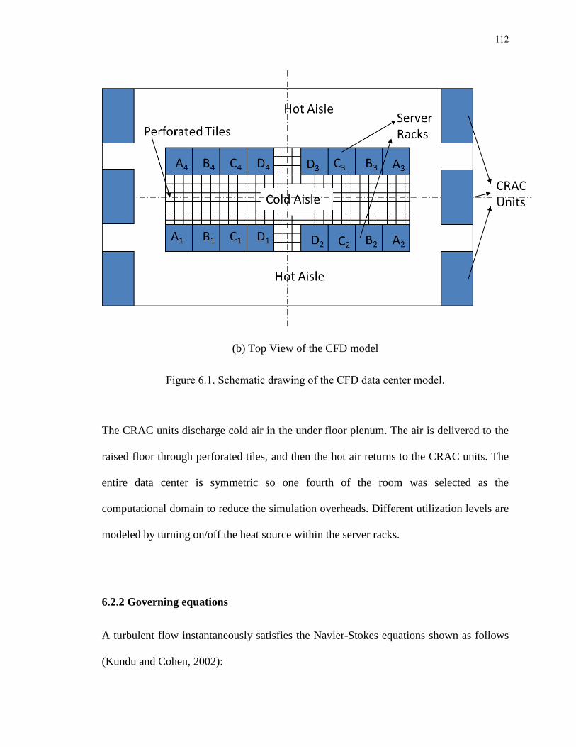
112

(b) Top View of the CFD model

Figure 6.1. Schematic drawing of the CFD data center model.

The CRAC units discharge cold air in the under floor plenum. The air is delivered to the

raised floor through perforated tiles, and then the hot air returns to the CRAC units. The

entire data center is symmetric so one fourth of the room was selected as the

computational domain to reduce the simulation overheads. Different utilization levels are

modeled by turning on/off the heat source within the server racks.

6.2.2 Governing equations

A turbulent flow instantaneously satisfies the Navier-Stokes equations shown as follows

(Kundu and Cohen, 2002):

113

0i

i

u

x

(6.1)

2

0 3[1 ( )]i i ij i

i i j j

u u p uu g T T

t x x x x

(6.2)

2

j

i j j

T T Tu

t x x x

(6.3)

However, it is a challenge to predict the flow in detail since there are different scales to

be resolved. The averaged equations are used to find to mean velocity and temperature of

a turbulence flow. The simplest “complete models” of turbulence are the two equation

models in which the solution of two separate transport equations allows the turbulent

velocity and length scales to be independently determined.

The turbulence kinetic energy and its rate of dissipation are obtained from the

following transport equations:

( ) ( ) [( ) ]ti k b M

i j k j

u G G Yt x x x

(6.4)

and

2

1 3 2( ) ( ) [( ) ] ( )ti k b

i j j

u C G C G Ct x x x k

(6.5)

where kG represents the generation of turbulence kinetic energy due to the mean velocity

gradient, calculated as:

114

' ' j

k i j

j

uG u u

x

(6.6)

bG is turbulence kinetic energy due to buoyancy. For ideal gas calculated as described:

Prb i

t i

G gx

(6.7)

MY represents the contribution of the fluctuating dilatation in compressible turbulence to

the overall dissipation rate:

22MY

a

(6.8)

In this study, the air is treated as incompressible flow, so this term is zero.

1C , 2C

,3C

are constants, k and

t are the turbulent Prandtl numbers for and ,

respectively. The corresponding values are 1.44, 1.92, 0.09, 1.0 and 1.3. Ansys Fluent

12.0 turbulent k-epsilon model was applied with standard wall functions was applied to

solve the equations listed above. The server rack is simplified as porous media with heat

source. The perforated tiles were treated as one dimensional porous jump boundary

condition. The pressure drop across the perforated tiles is expressed as:

2(0.5 )p K V (6.9)

where V is the velocity entering the perforated tile, and K is the flow resistance factor.

It was calculated by the equations given by Idelchik (1986):

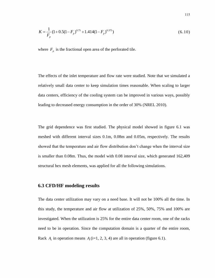
115

0.75 0.3751(1 0.5(1 ) 1.414(1 ) )p p

p

K F FF

(6.10)

where pF is the fractional open area of the perforated tile.

The effects of the inlet temperature and flow rate were studied. Note that we simulated a

relatively small data center to keep simulation times reasonable. When scaling to larger

data centers, efficiency of the cooling system can be improved in various ways, possibly

leading to decreased energy consumption in the order of 30% (NREL 2010).

The grid dependence was first studied. The physical model showed in figure 6.1 was

meshed with different interval sizes 0.1m, 0.08m and 0.05m, respectively. The results

showed that the temperature and air flow distribution don’t change when the interval size

is smaller than 0.08m. Thus, the model with 0.08 interval size, which generated 162,409

structural hex mesh elements, was applied for all the following simulations.

6.3 CFD/HF modeling results

The data center utilization may vary on a need base. It will not be 100% all the time. In

this study, the temperature and air flow at utilization of 25%, 50%, 75% and 100% are

investigated. When the utilization is 25% for the entire data center room, one of the racks

need to be in operation. Since the computation domain is a quarter of the entire room,

Rack 1A in operation means

iA (i=1, 2, 3, 4) are all in operation (figure 6.1).

116

(a)

(b)

(c)

(d)

Figure 6.2. Temperature distribution in the data center with 25% utilization.

racks are operating (b) racks are operating (c) Streamlines with operating (d)

Streamlines with operating.

Figure 6.2 shows the temperature distribution in the data center room with different racks

in operation. The CRAC inlet temperature is 20 ºC, and the flow rate for both cases is

3350CFM. When rack D is in operation (figure 6.2a), the maximum room temperature is

117

higher than the case that has the same utilization but with rack A in operation. This is

because rack D is further away from the air outlet, the hot air needs to travel longer time

in the room. Moreover, more vortexes are generated as it goes toward the outlet as shown

in figure 6.2c.

On the other hand, if rack A is operating, the hot air travels a shorter distance and the

CRAC system runs more efficiently, and the temperature distribution in the room ismore

uniformly distributed. Hence, in the following study, rack A will be operating when the

utilization is 25%.

(a)

(b)

(c)

(d)

Figure 6.3. Temperature distribution in the data center with 50% untilization.

118

(a) racks are operating, flow rate 4650CFM (b) racks are operating, flow

rate 5650CFM (c) racks are operating, flow rate 4650CFM (d) racks are

operating, flow rate 4650CFM

As the utilization increases to 50%, a higher flow rate is required to keep the tempeature

below a certain value. ASHRAE suggests that for most data centers, the high side

ambient temperature limit is 27°C, with an allowable limit of 32°C. Some data centers

are designed to work at warmer temperature between 27 to 32°C to save energy on

cooling, and some data centers are designed to operate at lower temperature for the better

performance of the equipment. In this study, we choose 30°C as the upper limit

temperature for the data center room. The CRAC system flow rate will be adjusted to

keep the maximum temperature under 30°C. The available flow rates are chosen from

Liebert Delux system/3, including 3350, 4650, 5650, 8400, 10200, 15200CFM. As shown

in figure 6.3a, when racks are operating, since the maximum temperature exceeds

30°C, the top of the racks and the CRAC outlet are the high temperature zones. The flow

rate is inscrease to 5650CFM to control the tempreature as shown in figure 6.3b. For 50%

utilization, the best case that meets the temperature requirement and saves energy is to

turn on rack with CRAC flow rate 4650CFM. The corresponding temperature

distribution is shown in figure 6.3d.

119

(a)

(b)

Figure 6.4. Streamlines for utilization 50%, are operating.

(a) velocity magnitude (b) temperature distrubtion

Base on our previous observation, it is beneficial for the temperature control and saving

energy to have rack A operating. When the utilization is increased, other racks will be

turned on accordingly. When the utilization is increased to 50%, the combination of

is the worst senario. This is because all the racks are further from the CRAC

outlet, and they are located between and racks, which block the air flow path and

lead to more local circulations before the hot air goes to the outside (figure 6.4). racks

are also in the middle comparing with rack, but they are closer to the outlet.

When the utilization is increase to 75%, if rack are operating, the flow rate has

to increase from 10200 to 12000 CFM to maintain the room temperature under 30°C

(figure 6.5 (a) and (b)). The combination of racks is the best case for 75%

120

utilization (figure 6.5(c)). When the utilization is 100%, the steady state temperature

distribution is shown in figure 6.5(d).

(c) 75% untilization

(d) 75% untilization

(e) 75% untilization

(f) 100% untilization

Figure 6.5. Temperature distribution with untilization 75% and 100%.

(a) racks are operating, flow rate 10200CFM (b) racks are operating,

flow rate 12000CFM (c) racks are operating, flow rate 10200CFM (d)

utilization 100%, all racks are operating, flow rate 12000CFM

121

The results from CFD/HF simulation can provide guidence for the data center operators

to choose the parameters that fit their own situations according to the heat load and the

capacity of the CRAC units and chillers.

6.4 Energy consumption

When the data center load is fixed, the total cooling energy consumed by the data center

is the sum of the work done by the CRAC and chiller. There are two main settings which

affect the cooling system’s energy consumption: the CRAC fan speed which determines

the air flow rate through the data center, and whether the chiller is turned on. Given an

outside temperature and a data center utilization level, the cooling system can be

designed to adjust the CRAC fan speed and chiller on/off setting to ensure not only the

operation reliability, but also to operate the data center in the most energy-efficient

manner.

The work done by CRAC fan is usually a linear function of the air flow rate, which can

be calculated as:

2.7CRAC inW V (6.11)

The chiller work is calculated by:

/chillerW Q COP (6.12)

122

The coefficient of performance(COP) of chiller-CRAC loop is a function of CRAC

supply temperature. The COP as a function of CRAC inlet temperature is applied in this

study:

2

s0.0068 0.0008 0.458sCOP T T ( 6 . 1 3 )

The higher the COP is, the less energy the chiller consumes.

If the outside temperature is sufficiently low, then the CRACs take the cold air from the

outside and discharge the hot air to the ambient. The chiller will be turned off in this case

to save energy. If the outside temperature is too high, then CRACs will need to circulate

the hot air through the chiller for cooling and send the cold air into the data center. In the

following section, total cooling energy consumption of the same data center at two

different locations will be presented and one can easily see that the cooling energy

consumption can change significantly throughout the day. Figures 6.6 to 6.8 are examples

to show the energy consumption corresponding to different boundary conditions.

Figure 6.6 shows the total energy consumption by the fan and chiller for different loads

during winter time in Seattle. Since the outside temperature is low enough, the chiller is

turned off. Hence, the energy consumed by chiller is zeros. Similarly, figure 6.7 shows

that the energy consumption for fan only during winter time in Princeton. Note that from

the equation 6.10 and 6.11, for the same amount of air flow, the chiller will consume

123

much more energy than the fan. Hence, the energy consumption during winter will be

reduced significantly.

124

Figure 6.6. The impact of outside temperature on energy consumption (Janurary, Seattle).

126

Figure 6.7. The impact of outside temperature on energy consumption (Janurary,

Princeton).

When the outside temperature is high, as shown in figure 6.8, simply increasing the flow

rate will not be able to maitain the low room temperature. In this case, the chiller needs to

be turned on to cool the air temperature down. When the load is 25%, with the lowest

127

available flow rate, the data center room temperature can be maintained below 30°C if

the CRAC supply temperature is at 24°C. During one day period showing in figure 6.8,

the chiller needs to be on if the outside temperature is higher than 24°C. The energy

consumed by the chiller takes from 30.4% to 72.4% of the total energy consumption.

128

Figure 6.8. The impact of outside temperature on energy consumption (August,

Princeton).

As the load is increased to 50%, the required CRAC supply temperature is at 20°C to

keep the data center room temperature below 30°C with air flow rate 5650CFM . The

chiller needs to be turned on all the time, and the total energy consumption is greatly

increased because of the work done by the chiller. For example, if the outside

temperature is 30.6°C, the chiller spends 75.2% of the total energy.

129

The energy consumption apparently does not vary linearly with the load increasement.

When the load is increased from 50% to 75%, with the same CRAC supply temperature,

the total energy consumption is increased about 49%. As the load keeps increasing to 100%

from 75%, the total energy consumption is only increased by 22%. Therefore, if one large

data center A has the same capacity as four small same-sized data centers , A is probably

consumes less energy than the sumb of the four B data centers. It is more enconomical to

build one large data center with high load capacity compared to several smaller ones.

The significant variability of cooling energy consumption versus temperautre and load

presents an interesting opportunity for dynamic load distribution to either minimize enrgy

consumption and/or cost. If a service is replicated across two data centers, one in

Northern California and one in Georgia, during the hottest and coolest periods of the day,

it might make sense to direct load to Georgia because the cooling energy consumed is

similar but the energy price might be lower in Georgia. On the other hand, when it is hot

in Georgia but cool in Northern California, it might be beneficial to direct more load to

Northern California because the cooling energy consumption will be much less.

While it makes sense to explore dynamic load distribution because of variable electricity

prices as well as cooling(Le. et al 2011), note that transient cooling effects need to be

carefully considered, which will be discussed in the next section.

130

6.5 Transient effects and pre-cooling

ASHRAE (2008) suggests that the recommended environment range of 18 to 27oC with

an allowable range from 15 to 32 oC for most data centers. Most data centers are running

with high temperature environment to minimize the cost. If there is a sudden load

increase, the cooling systems need a quick response and the CRAC systems have to be

able the handle the sudden change. For example, assume the CRAC system was on

standby mode, and ambient air was cold enough so it went through a bypass and served

directly to the under floor plenum room. When the load is suddenly increased, and a

lower supply temperature is required, the CRAC is switched to running mode with the

chiller turned on; it will experience a transient ramping period before it can completely

cool down the air.

There are two ways to decide the time for the CRAC system to become fully functional

numerically. One is to have the entire CRAC system details included in the CFD model

and monitor the time needed when the air flow coming out of the CRAC reaches the

required temperature. This might be more accurate, but will be very time consuming and

requires the detail drawing, dimension as well as materials of the CRAC system. The

other way is to use the lumped system analysis. It is relatively easy and simple. Moreover,

for the data center cooling system, it is preferable to have this number be conservative.

The time that is needed for the CRAC system and the air flow to reach the supply

temperature criterion (20ºC in this case) is estimated as follows:

131

exp( ) exp( )i

T T t t

T T RC

(6.14)

Where is the time constant,

p

s

c V

hA

(6.15)

Some assumptions and parameters are obtained by using the Liebert Delux system/3 (A

frame coil) shown in table 6.1. Based on the numbers obtained from the lumped system

analysis, the average response time for the CRAC system is assumed to be 20 minutes in

the following study.

Table 6.1. Response time for different flow rate.

Standard Air Volume-

CFM 3350 4650 5650 8400 10200 12000 15200

Weight-lbs (kg)-Deluxe

System/3

1455

(660)

1675

(760)

1690

(767)

2110

(957)

2280

(1034 )

2345

(1064)

2500

(1134)

Face Area-Sq. ft. (m2) 14.2

(1.32)

14.2

(1.32)

14.2

(1.32)

22.2

(2.06)

22.2

(2.06)

22.2

(2.06)

29.38

(2.73)

Rows of Coil 3 3 4 4 4 4 4

Time Constant (min) 14 17 13 10 11 11 9

Response time (to reach

80% of the required

temp) (min)

24 27 21 16 18 18 15

132

Different cooling responses (scenarios) for sudden load change occurring at t=0s were

listed in table 6.2. Each scenario is a sequence of different actions taken, which include

increasing the air flow, turning on the chiller or the combination of the two.

The initial conditions for all the scenarios are the same: the utilization was increased from

25% to 75% instantaneously. The chiller was off before the change and the flow rate was

3350 CFM. Since very little heat is lost from the system, if the cooling system settings

remain the same, the temperature will ramp up to 42ºC (the maximum temperature will

exceed 30 ºC in less than 5 minutes) with nearly all of the heat contributing to raise the

temperature as shown in figure 6.10 scenario 1. When the cooling level is increased, the

temperature rise will slowly decrease until a steady state temperature is again reached.

For scenario 2, the flow rate remained the same as the chiller was turned on right away at

t=0s, however, it will need about 20 minutes to respond. The initial response of scenario

2 is the same as scenario 1, except that the steady state temperature is lower as expected.

Table 6.2. Potential Responses of Cooling System to Sudden Large Load Increase.

Scenario 1 2 3 4 5

Time(min) t<20 t>20 t<20 t>20 t<20 t>20

Flow Rate (CFM) 3350 3350 10200 3350 10200 10200

Chiller OFF ON OFF ON ON

Flow go through

Chiller or not No No Yes No No Yes No Yes

133

Table 6.2(continued)

Scenario 6

Time

(min) t<5 5<T<10 t>10

Flow Rate (CFM) 3350 5650 10200

Chiller OFF

Flow go through Chiller or not No


Scenario 7

Time

(min) t<5 5<T<10 10<T<15 t>15

Flow Rate (CFM) 3350 5650 10200 15200

Chiller OFF

Flow go through Chiller or not No


Scenario 8

Time(min) t<5 5<T<10 10<T<15 t>15

Flow Rate (CFM) 3350 5650 10200 10200

Chiller OFF ON

Flow go through Chiller or not No Yes

134


Scenario 9

Time

(min) t<5 5<T<10 10<T<15 15<T<35 t>35

Flow Rate (CFM) 3350 5650 10200 10200 10200

Chiller OFF ON ON

Flow go through Chiller or not No Yes

Assuming that a maximum allowable operating temperature is 30ºC and the outside

temperature is 23 ºC, the only responses that eventually lead to a stable temperature under

30ºC are those that use the chiller. For example, scenario 3, which aggressively increases

the flow rate, stabilized the temperature at above 30ºC. Scenario 7, which ultimately uses

a larger flow rate than scenario 3, but increases the flow rate more conservatively is not

beneficial, allowing the temperature to rise over 32ºC before settling to a stable

temperature slightly above 30ºC.

t=8 min

t=16 min

135

t=25 min

t=33 min

t=41 min

t=58 min

Figure 6.9. Transient temperature distribution in the data center for scenario 2.

Furthermore, note that for scenario 4, 5 and 8, even though temperatures are either high

above the allowable temperature (scenario 4), or slightly higher than the allowable

temperature (scenario 5 and 8) as the load changed initially, the steady state temperature

of all the three scenarios are under 30ºC. Apparently, it is not sufficient to turn on the

chiller when the load change is observed. This will put the equipment under high risk and

may cause a break down because of the high temperature.

136

Figure 6.10. Temperature vs. time for different scenarios.

To prevent the overheating caused by the response time required by CRAC systems, pre-

cooling is proposed (Le. et al 2011). This part of the study is a collaboration with

researchers (Kien Le, Thu D. Nguyen, and Ricardo Bianchini) from the Department of

Computer Science here at Rutgers. If the arriving jobs exceed the capacity of current

cooling system settings and may cause overheating problem, they will be delayed or sent

to other data centers. The front-end can ask the data center to pre-cool (by turning on the

chiller early) in preparation for receiving load.

0 20 40 60 8025

30

35

40

Time (min)

Tem

per

atu

are(

oC

)

S1

S2

S3

S4

S5

S6

S7

S8

S9

137

(a) Scenario 4 with pre-cooling by 5 to 20 minutes

(b) Scenario 5 with pre-cooling by 5 to 20 minutes

0 20 40 60 80

25

30

35

40

Time (min)

Tem

per

atu

are(

oC

)

S4

Precooling 5 min

Precooling10 min

Precooling15 min

Precooling 20 min

0 20 40 60 80

25

30

35

40

Time (min)

Tem

per

atuar

e( o

C )

S5

Precooling 5 min

Precooling 10 min

Precooling 15 min

Precooling 20 min

138

(c) Scenario 8 with pre-cooling by 5 to 20 minutes

Figure 6.11. Temperature in the data center vs. different cooling responses.

The pre-cooling time depends on the cooling scenario setting. As shown in figure 6.12(a),

for scenario 4, even with 20 minutes pre-cooling, the temperature will still rise to 32ºC.

Scenario 5 (figure 6.11b), which immediately increases the flow rate as the chiller is

turned on, only needs to pre-cool for 5 minutes before the load change. For scenario

8(figure 6.11c), if you increase the flow rate gradually and meanwhile pre-cool for 10

minutes or longer, the temperature is controlled under 30ºC. It is unnecessary to pre-cool

the data center for 20 minutes for scenario 8.

0 20 40 60 80

25

30

35

40

Time (min)

Tem

per

atuar

e( o

C )

S8

Precooling 5 min

Precooling 10 min

Precooling 15 min

Precooling 20 min

139

Chapter 7 Conclusion

This chapter reviews the major conclusions of the dissertation. Electronic cooling

problems were investigated at both large scale and micro scale. The main results and

contributions of current study are listed below:

i. Comprehensive experimental and numerical study of microchannel heat sink

An experimental and numerical combined approach was applied to study the thermal and

fluid performance of microchannel heat sinks. Silicon microchannel heat sinks was

designed and fabricated. An experimental test facility was built and the data measurement

instruments were calibrated with a temperature measurement uncertainty within ±0.5

Multi-microchannel heat sinks of different geometries (straight, bended and branched

channels) were studied with varying flow rates and heat fluxes. The components that

contribute to the thermal resistance were identified and pressure drop was studied

including the inlet and outlet loses, developing flow losses, and frictional flow losses.

Numerical models were built for all heat sink devices experimentally tested and good

agreements between numerical and experimental results were discovered with disparity

within 4%. Vortices, secondary flow with mixing, and axial temperature gradient

enlargement were discovered as the flow changes direction in the bended and branched

channels through numerical simulation. Heat transfer is proven to be enhanced with

140

bended and branched channels, but with the trade-off of a higher pressure loss that

requires extra pumping power.

ii. Transient study

The transient heat transfer behavior of the multi-microchannel heat sinks with different

configurations (Straight channel, U-shaped channel and serpentine channel) was studied.

The experimental results suggested that the U-shaped channel heat sinks response faster

and remove heat more quickly compared with the straight channel and serpentine channel

heat sinks. The serpentine channel required more time to reach steady state compared

with straight channel. As the flow rate increased, the difference between the two

configurations became smaller. Varying heat flux had less impact on the response time

than varying flow rate. The response time results obtained from this study can be used as

one of the parameters to evaluate the thermal performance of heat sinks.

iii. Design and optimization

The optimization problems focused on two different designs: the straight and U-shaped

multi-microchannel heat sinks. The multi-objective optimization problems were

formulated and studied with and without physical constraints. For each example given in

this study, 125 sampling points were investigated. Various responses were generated

through parametric modeling of these data points to study the influence of flow rates and

geometrical variables to the thermal performances. The Pareto frontiers were found and

presented to demonstrate the trade-offs between the multi-objective functions. In the

141

constrained formulations, the feasible design spaces were narrowed and more

conservative optimal solutions were found. The developed strategies are useful not only

to understand the fundamental heat transfer and fluid flow characteristics in the multi-

microchannel designs, but also to provide quantitative inputs for the processes of design

and optimization.

iv. Data center cooling system

A detailed model of raised floor data center cooling system was developed. The cooling

power demand as a function of the data center load and outside temperature was obtained

with the maximum allowable temperature constraint. Since the energy consumption

varies significantly with outside temperature and the data center loads change

corresponding to dynamic load migration. The transient cooling effect corresponding to

an abrupt, large change in data center loads was investigated. The results suggested that

the pre-cooling before load increase is necessary in order to prevent overheating.

Different pre-cooling scenarios with different cooling demands were analyzed.

Future work

1. The enhancement in heat transfer due to the combination of different geometries can

be investigated. Combine different simple elements, such as L-bend, 90 bends, U-bends

Y-shaped channels and straight channels together to form a new heat sink design.

142

2. Study the enhancement of heat transfer with nano-particles with high conductivity

mixed in liquid. Understand the underlying physics of the effectiveness of the presence of

nano-particles.

3. Capture the local hot spot in the microchannel heat sink with fluorescence microscope,

and improve the thermal uniformity.

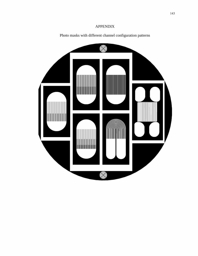
143

APPENDIX

Photo masks with different channel configuration patterns

145

BIBLIOGRAPHY

ASHRAE, 2008, “Environmental Guidelines for Datacom Equipment,” American

Society of Heating, Refrigeration, and Air-Conditioning Engineers

L. Deb, 2001, “Multi-Objective Optimization Using Evolutionary Algorithms of Wiley-

Interscience Series in Systems and Optimization”, John Wiley & Sons, LTD, Chichester,

England, pp. 50-57.

D. Abts, M. R. Marty, P. M. Wells, P. Klausler, and H. Liu, 2010, “Energy proportional

datacenter networks”, In ISCA 2010, pp338-347

V.K. Dwivedi, R. Gopal, S. Ahmad, 2000, “Fabrication of very smooth walls and

bottoms of silicon microchannels for heat dissipation of semiconductor devices”

Microelectronic Journal, Vol 31, pp405-410

A.G. Fedorov and R. Viskanta, 2000, “Three-dimensional Conjugate Heat Transfer in the

Microchannel heat sink for electronic packaging”, International Journal of Heat and Mass

Transfer, Vol. 43, pp. 399-415.

A. J. Ghajar and L. M. Tam, 1995, “Experimental Thermal and Fluid Science”, 10, pp

287-297

Guidelines for Evaluating and Expressing The Uncertainty of NIST Measurement Results,

1994, NIST Technical Note 1297.

S. Greenberg, E. Mills and B. Tschudi, etc. 2006, “Best Practices for Data Centers:

Lessons Learned from Benchmarking 22 Data Centers”, ACEEE Summer Study on

Energy Efficiency in Buildings.

T.M. Harms, M.J. Kazmierczak, and F.M. Gerner, 1999, “Developing Convective Heat

Transfer in Deep Rectangular Microchannels”, International Journal of Heat and Fluid

Flow, 210, 149-157.

146

A. Husain, K.Y. Kim, 2007, “Design optimization of microchannel for micro electronic

cooling”, The Fifth International Conference on Nanochannels, Microchannels and

Minichannels,. ICNMM2007-30053.

T. Harirchian, S.V. Garimella, 2008, “Microchannel size effects on local flow boiling

heat transfer to a dielectric fluid”, International Journal of Heat and Mass Transfer, Vol.

51 pp. 3724-3735.

I.E. Idelchik, 1986, Handbook of Hydraulic Resistance, 2nd ed., Harper & Row, New

York

International Technology Roadmap for Semiconductors (2008 update)

Y. Jaluria, 1998 , “Design and Optimization of Thermal System”.

R. C. Joy and E. S. Schlig, 1970, “Thermal Properties of Very Fast Transistors,” IEEE

Transactions on Electron Devices, Vol. ED-17, No.8, pp. 586-594

S. G. Kandlikar, 2003, “Microchannel and Minichannel-History, Terminology,

Classification and Current Research Needs” Paper No. ICMM 2003-1000 First

International Conference on Microchannels and Minichannels 2003, April 24-25,

Rochester. NY

K. C., Karki, A. Radmehr,and S. V. Patankar, 2003, “Use of Computational Fluid

Dynamics for Calculating Flow Rates Through Perforated Tiles in Raised-Floor Data

Centers,” International Journal of Heating, Ventilation, Air-Conditioning, and

Refrigeration Research, 9(2):153-166.

P. K. Kundu, and I. M Cohen, 2002: Fluid Mechanics. 2nd ed. Elsevier Academic.

K. Le, J. Zhang, J. Meng, R. Bianchini, T. D. Nguyen, Y. Jaluria, 2011, “Reducing

Electricity Cost Through Virtual Machine Placement in High Performance Computing

Clouds”, Proceedings of Super Computing (SC11)

147

J. Li, G. P. Peterson, P. Cheng, 2004, “Three dimensional analysis of heat transfer in a

micro-heat sink with single phase flow”. International Journal of Heat and Mass Transfer,

47 4215-4231.

Z. Li, X. Huai, Y. Tao and H. Chen, 2007, “Effects of thermal property variations on the

liquid flow and heat transfer in microchannel heat sinks”, Applied. Thermal Engineering.

27 (2007), pp. 2803–2814.

P. T. Lin, H. C. Gea, and Y. Jaluria, 2010, "Systematic Strategy for Modeling and

Optimization of Thermal Systems with Design Uncertainties". Frontiers in Heat and

Mass Transfer, 1, Paper number 013003.

G.M. Mala, D. Li, C. Werner, H.J. Jacobasch, and Y.B Ning, 1997, “Flow Characteristics

of Water through Microchannels Between Two Parallel Plates with Electrokinetic Effects

International Journal of Heat and Fluid Flow, 18, 489-496.

G. Maranzan, I. Perry, and D. Maillet, 2004, “Mini-and Micro-channels: Influence of

axial conduction in the walls" International Journal of Heat and Mass Transfer, Vol.47,

pp. 3993-4004.

NREL, 2010, “Best Practices Guide for Energy-Efficient Data Center Design,” National

Renewable Energy Laboratory (NREL), U.S. Department of Energy

I. Papautsky, J. Brazzle, T. Ammel, and A.B. Frazier, 1999, “Laminar Fluid Behavior in

Microchannels Using Micropolar Fluid Theory”, Sensors and Actuators, 73, 101-108.

Parker Hannifin Corp., "Data Sheet of Miniature Diaphragm Pumps: LTC Series

650mLPM Free Flow Mini Pumps (liquids)". See also URL http://www.parker.com/

precisionfluidics.

M. Patterson, “The effect of Data Center Temperature on Energy Efficiency”, Thermal

and Thermomechanical Phenomena in Electronic Systems, 2008, pp1167-1174.

K. E. Petersen, 1982, “Silicon as a mechanical Material”, Proceedings of the IEEE, Vol.

70. No.5 pp. 420-457

148

T. Sato, 1967, “Spectral Emissivity of Silicon”, Jpn. J. Appl. Phys. 6. Pp.339-347

R. Schmidt, 2004 “Raised-Floor Data Center: Perforated Tile Flow Rates For various Tile

Layouts”, 2004, Inter Society Conference on Thermal Phenomena “.

R. K. Shah, A. L. London, 1978, ‘Laminor Flow Froced Convection in Ducts’, Academic

Press, INC

P. Sharath, C. Rao, M.M. Rahman, and H.M Soliman, 2006, “Numerical Simulation of

Steady-State Conjugate Heat Transfer in a Circular Microtube inside a Rectangular

Substrate”, Numerical Heat Transfer, Part A, Vol.49, pp. 635-654, 2006.

M. E. Steinke, S. G. Kandikar et al, 2006, “Development of An experimental facility for

investigating single phase liquid flow in microchannels”, Heat Transfer Engineering, 27

(4):pp. 41-52.

W. Tschudi, P. Sreedharan, T. Xu, D. Coup, P. Roggensack, 2003, “Data Centers and

Energy Use” paper No.162 American Council for an Energy-Efficient Economy report.

C.P. Tso, and S.P. Mahulikar, , 1998, “The Use of the Brinkman Number for Single

Phase Forced Convective Heat Transfer in Microchannels”, International Journal of Heat

and Mass Transfer, 41, 12, 1759-1769.

D. B. Tuckerman, and R.F.W. Pease, 1981, “High Performance Heat Sinking for VLSI,

IEEE Electronic Device” Lett. EDL_2 126-129

D.B. Tuckerman, 1984, “Heat-Transfer Microstructures for Integrated Circuits, ” Ph. D.

Thesis, Stanford University, Stanford, CA

Y. Wang, P. Jackson, T. Phaneuf, 2009, “Flow structure in a U-shaped Channel”, Journal

of Thermophysics and Heat Transfer, Vol.23 no.1 (106-119).

149

X. J. Wei, Y. K. Joshi, 2004, “Stacked microchannel heat sinks for liquid cooling of

microelectronic components”, Journal of Electronic Packaging 126, 60

C. L. Wiginton, C. Dalton, “Incompressible laminar flow in the entrance region of a

rectangular duct”. Journal of Applied Mechanics. 37, 854-359

R. Xiong, J. Chung, 2007, “Flow characteristics of water in straight and serpentine micro-

channels with miter bends”, Experimental Thermal and Fluid Science 31, 805-812.

L. Zhang, J. Koo, L. Jiang, M. Asheghi, K, Goodson, J. Santiago, T. Kenny, 2002,

“Measurements and Modeling of Two-phase Flow in Microchannels With Nearly

Constant Heat Flux Boundary Conditions”

H.Y. Zhang, D. Pinjala, T.N. Wong, K.C. Toh and Y.K. Joshi, 2005, “Single-phase liquid

cooled microchannel heat sink for electronic packages”, Applied. Thermal Engineering.

25 pp. 1472–1487.

X. Zhang, J. VanGilder, M, Iyengar, R. Schmidt, “Effect of Rack Modeling Detail of the

Numerical Results of a Data Center Test Cell”. Thermal and Thermomechanical

Phenomena in Electronic Systems, 2008. THERM 200831, pp1183-1190

cooling of electronic system: jingru zhang a …

Documents