cooperative robot control and concurrent … · cooperative robot control and concurrent ......
TRANSCRIPT

1
Cooperative Robot Control and ConcurrentSynchronization of Lagrangian Systems
Soon-Jo Chung, Member, IEEE, and Jean-Jacques Slotine
Abstract—Concurrent synchronization is a regime where di-verse groups of fully synchronized dynamic systems stably coex-ist. We study global exponential synchronization and concurrentsynchronization in the context of Lagrangian systems control.In a network constructed by adding diffusive couplings torobot manipulators or mobile robots, a decentralized trackingcontrol law globally exponentially synchronizes an arbitrarynumber of robots, and represents a generalization of the averageconsensus problem. Exact nonlinear stability guarantees andsynchronization conditions are derived by contraction analysis.The proposed decentralized strategy is further extended toadaptive synchronization and partial-state coupling.
I. INTRODUCTION
Distributed and decentralized synchronization phenomenaof large dynamic groups are areas of intense research. In thisarticle, synchronization is defined as a complete match of allconfiguration variables of each dynamic system such that x1 =x2 = · · · = xp and p denotes the number of sub-systems in thenetwork. While such a definition directly concerns the angularposition synchronization problem, this paper also addressesthe synchronization of biased variables with application to thetranslational position coordination problem. In the latter case,synchronization corresponds to y1 = y2 = · · · = yp where yi,1 ≤ i ≤ p connotes a vector of biased variables constructedfrom the configuration vector xi such that yi(t) = xi(t) +bi(t) and the separation vector bi(t) is independent of thedynamics. Furthermore, we construct complex robot networkswhere multiple groups of fully synchronized elements coexist.Such concurrent synchronization seems pervasive in biology,and in particular in the brain where multiple rhythms coexistand neurons can exhibit many qualitatively different types ofoscillations [32].
The objective of this paper is to establish a unified syn-chronization framework that can achieve both the synchro-nization of the configuration variables of the robots and thestable tracking of a common desired trajectory. Althoughan uncoupled trajectory tracking control law, in the absenceof external disturbances, would achieve synchronization to acommon desired trajectory, non-identical disturbances justifythe mutual synchronization of the system variables. On theother hand, the synchronization to the average of initialconditions is not sufficient for multi-robot or multi-vehiclesystems where a desired trajectory is explicitly given. For
Assistant Professor of Aerospace Engineering, Iowa State University, Ames,IA 50011, E-mail: [email protected].
Professor of Mechanical Engineering & Information Sciences, Professorof Brain & Cognitive Sciences, Massachusetts Institute of Technology, Cam-bridge, MA 02319, E-mail: [email protected].
example, a large swarm of robots can first synchronize theirattitudes and positions to form a certain formation pattern,then track the common desired trajectory to accomplish thegiven mission. In production processes, such as manufacturingand automotive applications, where high flexibility, manipu-lability, and maneuverability cannot be achieved by a singlesystem [36], there has been widespread interest in cooperativeschemes for multiple robot manipulators that track a prede-fined trajectory. A stellar formation flight interferometer [8],[9] is another example where precision control of relativespacecraft motions is indispensable. The proposed synchro-nization tracking control law can be implemented for suchpurposes, where a common desired trajectory can be explicitlygiven. The proposed strategy can achieve more efficient androbust performance through local interactions, especially inthe presence of non-identical external disturbances. Further,we generalize the proposed control law such that multipledynamic systems can synchronize themselves from arbitraryinitial conditions without the need for a common referencetrajectory. As a result, other potential applications includeoscillation synchronization of robotic locomotion [33], [37],and tele-manipulation of robots [3], [27].
The main contributions of this work can be stated as follows.• Concurrent synchronization that exploits the multiple
time scale behaviors from two types of inputs (a referencetrajectory and local couplings) permits construction of acomplex time-varying network comprised of numerousheterogeneous systems.
• In contrast with prior work on consensus and flockingproblems using graphs, the proposed strategy primarilydeals with dynamic networks consisting of nonlineartime-varying dynamics.
• We use contraction analysis [24], [45] as our main nonlin-ear stability tool, thereby deriving exact and global resultswith exponential convergence, as opposed to asymptoticconvergence of prior work.
• The proposed control laws are of a decentralized formrequiring only local velocity/position coupling feedbackfor global exponential convergence, thereby facilitatingimplementation in real systems.
• The theory is generalized and extended to multi-robotsystems with non-identical dynamics, linear couplingcontrol, partial state coupling, uni-directional coupling,and adaptive control.
A. Comparison with Related WorkThe consensus problems on graph [28] and the coordination
of multi-agent systems [15], [23], [29], [30] are closely
arX
iv:0
711.
1709
v4 [
mat
h.O
C]
18
Nov
200
8

2
related with the synchronization problem. In particular, theuse of graph theory and Laplacian produced many interestingresults [15], [20], [23], [26], [28], [34], [35]. However, thesynchronization to the average of initial conditions mightnot be directly applicable to multi-robot and multi-vehiclesystems, where a desired trajectory is explicitly defined. Arecent work [34] studied the consensus problem with a time-varying reference state, based on a single integrator model. Inessence, the aforementioned work mainly deals with simpledynamic models such as linear systems and single or doubleintegrator models without nonlinearly coupled inertia matrices.In contrast, we aim at addressing highly nonlinear systems(e.g. helicopters, attitude dynamics of spacecraft, walkingrobots, and manipulator robots). As shall be seen later, theproof of the synchronization for network systems that possessnonlinearly coupled inertia matrices is more involved. Thispaper focuses on such dynamic networks consisting of highlynonlinear systems.
One notable work [36] introduced a nonlinear trackingcontrol law that synchronized multiple robot manipulators inorder to track a common desired trajectory. Due to its all-to-allcoupling requirement, the number of variables to be estimatedincreases with the number of robots to be synchronized, whichimposes a significant communication burden. Additionally, thefeedback of estimated acceleration errors requires unnecessaryinformation and complexity. Thus, a method to eliminateboth the all-to-all coupling and the feedback of the accelera-tion terms is explored in this paper. Another nice approachto the synchronization of robot networks is to exploit thepassivity of the input-output dynamics [3], [4]. Its propertyof robustness to time delays is particularly attractive, whilerobot dynamics are passive only with velocity outputs unlesscomposite variables are employed. In addition, the mutualsynchronization problem, which not only synchronizes thesub-members but also enforces them to follow a commonreference trajectory, is not addressed. In particular, it shallbe shown that our proposed control law generalizes the robotcontrol law presented in [4], while our convergence result isstronger (exponential). One recent work [14] used the passivityproperty for the path-following system to synchronize the pathvariables. The passive decomposition [19], [20] describes astrategy of decoupling into the internal group formation shapeand the total group maneuver. Due to its dependency on acentralized control architecture, the decoupling is not generallyensured under the decentralized control. [20] considers lineardouble integrator models. Another work [11] proposed a nicecontrol framework for controlling and coordinating a groupof nonholonomic mobile robots, although the exact synchro-nization of individual vehicles was not pursued. One recentwork [31] presented a framework called particles with coupledoscillator dynamics so that collective spatial patterns emerge.Our recent work [9] also discussed more complex spacecraftdynamics to achieve the phase synchronization of spiral orcircular translational trajectories in three dimensions as wellas the synchronization of rotational dynamics. Also, it isimportant to note that the adaptive synchronization of multiplerobotic manipulators in a single local coupling configurationwas studied in [43], [44].
The proposed synchronization framework using contractionanalysis, first reported in [6], has a clear advantage in its broadapplications to a larger class of identical or nonidentical non-linear systems even with complex coupling geometry includinguni-directional couplings and partial degrees-of-freedom cou-plings, non-passive input-output, and time delays [7], [46],while ensuring a simple decentralized coupling control law(see Figure 1 for network structures permitted here). Theproofs and new results from [6] are expanded in this paper.In particular, concurrent synchronization that exploits twodifferent types of inputs has not been studied in the literature.
B. Organization
Section II describes modeling of robots based on theLagrangian formulation, and summarizes the key stabilitytheorems. While Section III presents the main control lawand its tracking stability, the proof of exponential synchro-nization is more involved and treated separately in SectionIV. The remainder of the paper further highlights the uniquecontributions of this work. Section V elucidates the concurrentsynchronization of complex networks and the leader-followerproblem. The main idea of this paper is extended to linearProportional-Derivative (PD) couplings, and limited partial-state couplings in Section VI. Key simulation results are alsopresented in Section VI.
II. MODELING AND NONLINEAR STABILITY TOOLS FORMULTI-ROBOT NETWORKS
A. Lagrangian Systems
This paper is devoted to the use of the Lagrangian for-mulation for its simplicity in dealing with complex systemsinvolving multiple dynamics. The equations of motion fora robot with multiple joints (qi ∈ Rn) can be derived byexploiting the Euler-Lagrange equations:
Li =12qT
i Mi(qi)qi−Vi,d
dt
∂Li(qi, qi)∂qi
− ∂Li(qi, qi)∂qi
= τi
(1)where i, (1 ≤ i ≤ p) denotes the index of robots or dynamicsystems comprising a network, and p is the total number ofthe individual elements. Equation (1) can be represented as
Mi(qi)qi + Ci(qi, qi)qi + gi(qi) = τi (2)
where gi(qi) = ∂Vi
qi, and, τi is a generalized force or torque
acting on the i-th robot.Note that we define Ci(qi, qi) such that (Mi − 2Ci) is
skew-symmetric [38], and this property plays a central role inour stability analysis using contraction theory [7].
The following key assumptions are used throughout thispaper. Since the main applications of the present paper includefully actuated robot manipulators and spacecraft [9], the robotsystem in (2) is fully actuated. In other words, the number ofcontrol inputs is equal to the dimension of their configurationmanifold (= n). The mass-inertia matrix M(q) is assumed tobe uniformly positive definite, for all positions q in the robotworkspace [38].

3
B. Contraction Analysis for Global and Exponential Stability
(1) Modular Stability Analysis: Although one popular methodfor modular stability analysis is to exploit the passivity formal-ism [38], we use contraction theory [24], [32], [39], [45] asan alternative tool for analyzing modular stability of couplednonlinear systems. In particular, contraction analysis has moregeneral and intuitive combination properties (e.g., hierarchies)than the passivity method, since it involves a state-space ratherthan an input-output method.(2) Differential State-State Analysis: Lyapunov’s linearizationmethod indicates that the local stability of the nonlinear systemcan be analyzed using its differential approximation. What isnew in contraction theory is that a differential stability analysiscan be made exact, thereby yielding global results on the time-varying nonlinear system.(3) Stronger Stability Results (Exponential and Global): Fora robot dynamic model in (2) and a time-varying trackingcontrol law, the straightforward use of Barbalat’s lemma orLaSalle-Yoshizawa theorem [18] yields asymptotic conver-gence results. While global exponential stability can be provenby using a Lyapunov function with a cross-term and additionalconstraints [1], [2], [17], such a method is ad hoc, as comparedto contraction theory. While exact exponential convergencemight not be achievable in real systems due to the modelingerrors, we believe that finding an explicit convergence ratewith exponential stability, if possible, is important due to itssuperior tracking performance and property of robustness withrespect to perturbations (e.g., see p. 339–350 in [17]).
A brief review of the results from [24], [39], [45] ispresented in this section. Note that contraction theory is ageneralization of the classical Krasovskii’s theorem [38], andthat approaches closely related to contraction, although notbased on differential analysis, can be traced back to [10], [13]and even to [22].
Consider a smooth nonlinear system
x(t) = f(x(t),u(x, t), t) (3)
where x(t) ∈ Rn, and f : Rn × Rm × R+ → Rn. A virtualdisplacement, δx is defined as an infinitesimal displacementat a fixed time– a common supposition in the calculus ofvariations.
Theorem 1: For the system in (3), if there exists a uniformlypositive definite metric,
M(x, t) = Θ(x, t)T Θ(x, t) (4)
where Θ is some smooth coordinate transformation of thevirtual displacement, δz = Θδx, such that the associatedgeneralized Jacobian, F is uniformly negative definite, i.e.,∃λ > 0 such that
F =(
Θ(x, t) + Θ(x, t)∂f∂x
)Θ(x, t)−1 ≤ −λI, (5)
then all system trajectories converge globally to a single tra-jectory exponentially fast regardless of the initial conditions,with a global exponential convergence rate of the largesteigenvalues of the symmetric part of F.
Such a system is said to be contracting. The proof is given in[24]. Equivalently, the system is contracting if ∃λ > 0 suchthat
M +(∂f∂x
)T
M + M∂f∂x≤ −2λM (6)
Equation (6) is useful for the stability proof of a Lagrangiansystem, since the inertia matrix M(q) of the robot dynamicsin (2) can be chosen as the metric M in (6).
The key advantage of contraction analysis is its superiorcombination property as follows.
C. Contraction of Coupled Systems
The following theorems are used to derive stability andsynchronization of coupled Lagrangian systems.
Theorem 2: Hierarchical combination [39]. Consider twocontracting systems, of possibly different dimensions and met-rics, and connect them in series, leading to a smooth virtualdynamics of the form
d
dt
(δz1
δz2
)=(
F11 0F21 F22
)(δz1
δz2
)Then, the combined system is contracting if F21 is bounded.
Proof: see [7], [39], [40].Theorem 3: Partial contraction [45]. Consider a nonlinear
system of the form x = f(x,x, t) and assume that the auxiliarysystem y = f(y,x, t) is contracting with respect to y. If aparticular solution of the auxiliary y-system verifies a specificsmooth property, then all trajectories of the original x-systemverify this property exponentially. The original system is saidto be partially contracting.
Proof: See [45] for the virtual observer-like y system.Theorem 4: Synchronization [45]. Consider two coupled
systems. If the dynamics equations verify
x1 − f(x1, t) = x2 − f(x2, t)
where the function f(x, t) is contracting in an input-independent metric, then x1 and x2 will converge to eachother exponentially, regardless of the initial conditions. Math-ematically, stable concurrent synchronization corresponds toconvergence to a flow-invariant linear subspace of the globalstate space [32].
Proof: This can be proven by constructing the virtualsystem y− f(y, t) = u(t) and using Theorem 3 (see [45]).
Remark 1: Whereas Theorem 2 can be proven for differentmetrics, Theorem 4 requires the same metric (e.g., inertiamatrix) among the coupled systems. Hence, Theorem 4 cannotbe directly applied to coupled Lagrangian systems. This isone of the motivations of the current paper, and elucidated inSection IV.
III. CONTROL LAW AND ITS TRACKING STABILITY
A tracking controller introduced in this section achieves notonly global exponential synchronization of the configurationvariables, but also global exponential convergence to thedesired trajectory.

4
211
54 3
4
21 2
3
(a) with bi-directional couplings
4
1
4 3
121
223
5
(b) heterogeneous robots
2
1
4
21
3 31
5 4
2
3
(c) with uni-directional couplings
2
1
3 4
6
5
4
21
3
(d) with uni-directional and bi-directional couplings
4 3
21
8 7
65
2
1
3
4
7
5
6
(e) unbalanced graphs with feedback hierarchies
5
3
21
6 4
9
10
8
7
1
2
3
(f) inline configuration
Fig. 1. Network structures permitted in this paper. Networks in (a-d) areon balanced graphs, and each element has the same number of neighbors(i.e, regular graph). More complex structures, such as the unbalanced graphsshown in (e), can be constructed by concurrent synchronization presented inSection V. The solid lines indicate the local couplings, whereas the dash linesindicate the reference input commands.
A. Proposed Synchronization Control Strategy
Let us first consider the robot networks shown in Fig. 1(a-d). The following control law, adopted from the single robotcontrol law in [38], is proposed for the i-th robot in a networkcomprised of p robots (p ≥ 3).
τi =M(qi)qi,r + C(qi, qi)qi,r + g(qi) (7)
−K1(t)(qi − qi,r) +m∑
j∈Ni(t)
2m
K2(t)(qj − qj,r)
which also permits the uni-directional couplings shown inFigures 1 (c) and (d). Note that m, which is the same for eachrobot, is the number of its neighbors that send the couplingsignals to the i-th member, and the constant or time-varyingset Ni(t) consists of such neighbors. This generalized formwill be discussed again in Section V.
Equation (7) reduces to the following tracking controllaw for a two-way-ring symmetric structure, as shown inFigure 1(a)
τi =M(qi)qi,r + C(qi, qi)qi,r + g(qi)−K1(t)(qi − qi,r)+ K2(t)(qi−1 − qi−1,r) + K2(t)(qi+1 − qi+1,r) (8)
where a uniformly positive definite matrix K1(t) ∈ Rn×n
is a feedback gain for the i-th robot, and another uniformlypositive definite matrix K2(t) ∈ Rn×n is a coupling gain withthe adjacent members (i− 1 and i+ 1). While (8) constructsa closed graph (e.g., ring), an inline configuration is alsopermitted since the first and last robot can simply connect theK2(t) gain from itself (see Fig. 1(f) and Section V-A). Theabove control law can also be applied to a network consistingof p non-identical robots (Figure 1(b)), as shall be seen inSection V-B.
While the common desired time-varying trajectory (or thevirtual leader dynamics) is denoted by qd(t), the referencevelocity vector, qi,r is given by shifting the common desiredvelocity qd with the position error:
qi,r = qd −Λqi = qd −Λ(qi − qd) (9)
where Λ is a positive diagonal matrix.In contrast with [36], the proposed control law requires onlythe local coupling feedback of the most adjacent robots (i− 1and i + 1) for exponential convergence (see Figure 1). Notethat the last (p-th) robot is connected with the first robot toform a ring network as suggested in [45]. Moreover, estimatesof q are no longer required.
The closed-loop dynamics using (2) and (8) become
M(qi)si +C(qi, qi)si +K1si−K2si−1−K2si+1 = 0 (10)
where si denotes the composite variable si = qi − qi,r.
B. Modified Laplacian
Let us define the following p× p block square matrices:
[LpA,B] =
A B 0 ··· BB A B ··· 0...
. . . . . ....
0 B A BB ··· 0 B A
p×p
, [UpA] =
A A ··· AA A ··· A...
.... . .
...A A ··· A
p×p
For a ring structure, defined from the controller in (8), [LpA,B]
has only three nonzero matrix elements in each row (i.e.,A,B,B). Then, we can write the closed-loop dynamics in(10) in the following block matrix form
[M]x + [C]x +([Lp
K1,−K2] + [Up
K2])
x = [UpK2
]x (11)
where [M] = diag (M(q1), · · · ,M(qp)),[C] = diag (C(q1, q1), · · · ,C(qp, qp)), x =
(sT1 , · · · , sT
p
)T.
Definition [LpK1,−K2
] can be viewed as the modified Lapla-cian of the network in the context of graph theory. In otherwords, [Lp
K1,−K2] indicates the connectivity with adjacent
systems as well as the strength of the coupling by K2. Notethat [Lp
K1,−K2] can be time-varying due to time-varying K1
and K2, or due to the switching topology, Ni(t) in (7).
Remark 2: The network graphs illustrated in Figure 1(a-d) are balanced since the in-degree of each node is equalto the out-degree [28]. The additional requirement for thestability analysis in this section is that the robots shouldbe on a regular graph, where each member has the samenumber of neighbors. While this paper permits popular localcoupling configurations [9], [15] from regular graphs, we willshow that the assumption of a regular balanced graph can berelaxed in Section V. In particular, unbalanced or non-regulargraphs due to feedback hierarchies, as shown in Figure 1(e),can be employed by concurrent synchronization discussed inSection V.
Remark 3: It should be noted that the matrix [LpK1,−K2
]is different from the standard Laplacian found in [28]. Bydefinition, every row sum of the Laplacian matrix on abalanced graph is zero. Hence, such Laplacian matrix alwayshas a zero eigenvalue corresponding to a right eigenvector,
5
1 = (1, 1, · · · , 1)T . In contrast, a strictly positive definite[Lp
K1,−K2] is required for exponential tracking convergence
for the proposed control law in this paper. In other words,unless otherwise noted, [Lp
K1,−K2] is assumed to have no zero
eigenvalue. For example, the block matrix for p = 4 becomes
[L4K1,−K2
] =
[+K1 −K2 0 −K2−K2 +K1 −K2 0
0 −K2 +K1 −K2−K2 0 −K2 +K1
](12)
which is positive definite for K1 − 2K2 > 0. This conditionis also true ∀p, p ≥ 3.
C. Tracking Stability Analysis
The following condition should be true for exponentialtracking convergence to the common desired trajectory qd(t).
Theorem 5: If [LpK1,−K2
] is uniformly positive definite:
[LpK1,−K2
] > 0, ∀t (13)
then every robot follows the desired trajectory qd(t) exponen-tially fast from any initial condition.
Proof: We can cancel out the [UpK2
] matrix term in (11)to obtain
[M]x + [C]x + [LpK1,−K2
]x = 0. (14)
Equation (14) corresponds to a conventional tracking problemwith a block diagonal matrix of nonlinearly coupled inertiamatrices, [M]. We use contraction theory to prove that xtends to zero exponentially and globally with [Lp
K1,−K2] > 0.
Consider the virtual system of y obtained by replacing x withy in (14).
[M]y + [C]y + [LpK1,−K2
]y = 0 (15)
This virtual y system has two particular solutions: x =(sT
1 , · · · , sTp )T and 0. The squared-length analysis with respect
to the positive-definite metric [M] yields
d
dt
(δyT [M]δy
)= 2δyT [M]δy + δyT [M]δy (16)
= −2δyT([C]δy + [Lp
K1,−K2]δy)
+ δyT [M]δy
= −2δyT [LpK1,−K2
]δy
where we used the skew-symmetric property of [M]− 2[C].Accordingly, [Lp
K1,−K2] > 0 will make the system contract-
ing (δy → 0), thus all solutions of y converge to a singletrajectory globally and exponentially fast (Theorems 1 and3). This in turn indicates that the composite variable of eachrobot tends to zero exponentially (si → 0). By definition ofsi = qi − qd + Λ(qi − qd), this show global exponentialconvergence of qi to the common reference trajectory qd(t)(see also Theorem 2).
Given K1 > 0,K2 > 0, it can be shown that a sufficientcondition for the positive-definiteness of [Lp
K1,−K2] is K1 −
K2 > 0 for p = 2, and K1 − 2K2 for p ≥ 3.The next question to be addressed is how to guarantee the
synchronization of the individual dynamics.
IV. SYNCHRONIZATION WITH/WITHOUT TRACKING
We prove the exponential synchronization of multiple La-grangian systems in this section. First, we describe the diffi-culties inherent in proving the synchronization of Lagrangiansystems in Section IV-A. We then present the synchronizationproof in Sections IV-C. We also show that our method is moregeneral than prior work by reducing our control law to thestandard synchronization problem without trajectory trackingin Section IV-D. The adaptive synchronization is presented inSection IV-E.
A. Challenges with Nonlinear Inertia Matrix
The difficulties associated with nonlinear time-varying in-ertia matrices can be easily demonstrated with the followingtwo-robot example. The closed-loop dynamics of two identicalrobots from (10) becomes
M(q1)s1 + C(q1, q1)s1 + (K1 + K2)s1 = u(t)M(q2)s2 + C(q2, q2)s2 + (K1 + K2)s2 = u(t)
(17)
Note that u(t) = K2(s1 + s2) and that si, i = 1, 2 is thecomposite variable defined in (10).
Direct application of synchronization (Theorem 4) appearselusive since we have to prove that (17) are contracting inthe same metric while preserving the input symmetry [32].Hence, this can be viewed as a higher order contractionproblem [25]. For example, multiplying (17) by M−1 breaksthe input symmetry: i.e., M−1(q1)u(t) 6= M−1(q2)u(t). Inessence, M(q1) 6= M(q2) makes this problem intractable ingeneral.
Instead, assume that M(q) becomes a constant matrix,thereby making C(q, q) zero. Then, we can easily prove s1
and s2 tend to each other from
Ms1 + (K1 + K2)s1 = u(t), Ms2 + (K1 + K2)s2 = u(t)(18)
The following virtual y-system with the common input u(t)
My + (K1 + K2)y = u(t) (19)
is partially contracting with K1 + K2 > 0 (see Theorem 3).Hence, its particular solutions s1 and s2 tend to each otherexponentially fast according to the synchronization theorem(Theorem 4). Without loss of generality, this result can easilybe extended to arbitrarily large networks. The synchronizationof a large network with a constant metric, as seen in (18), isalready discussed in [45] using contraction analysis.
We now turn to a more difficult problem focused on thesynchronization of two robots with non-constant nonlinearmetrics (M(q1) 6= M(q2)).
B. Contraction with Multiple Time Scales
In this section, we show that we can render the systemsynchronized first, then follow the common trajectory bytuning the gains properly. This indicates that there exist twodifferent time scales in the closed-loop systems constructedwith the proposed controllers. This multi-time-scale behaviorwill be exploited in the subsequent sections.
6
Recall the closed-loop dynamics given in (14). Since[Lp
K1,−K2] is a real symmetric matrix, we can perform the
spectral decomposition [5]. This is a special case of the con-current synchronization [32] that corresponds to convergenceto a flow invariant subspace (the eigenspace).
[LpK1,−K2
] = V[D]VT (20)
where [D] is a block diagonal matrix, and the square matrixV is composed of the orthonormal eigenvectors such thatVT V = VVT = Ipn, since the symmetry of [Lp
K1,−K2] gives
rise to real eigenvalues and orthonormal eigenvectors [42].Pre-multiplying (14) by VT and setting VT x = z result in(
VT [M]V)z +
(VT [C]V
)z + [D]z = 0 (21)
Then, we can develop the squared-length analysis, as in(16). This follows from the fact that
(VT [M]V
)is always
symmetric positive definite due to a symmetric positive defi-nite [M].
Since the modified Laplacian [LpK1,−K2
] represents a reg-ular graph, where each member has the same number ofneighbors (= 2 for p ≥ 3),
[1] =1√p[In, In, · · · , In]T (22)
is the pn× n block column matrix of eigenvectors associatedwith the eigenvalues λ(K1 − 2K2) for p ≥ 3. Note that In
denotes the n× n identity matrix, and the [1] matrix consistsof p matrices of In. The eigenvector matrix [1] represents thecommon reference trajectory tracking state.
We can define a pn× (p− 1)n matrix Vsync that consistsof the orthonormal eigenvectors other than [1] such that
VT V =(
[1]T
VTsync
)([1] Vsync
)(23)
=[
[1]T [1] [1]T Vsync
VTsync[1] VT
syncVsync
]=[
In 0n×(p−1)n
0(p−1)n×n I(p−1)n
]where we used the orthogonality between [1] and Vsync.
Hence, the block diagonal matrix [D], which represents theeigenvalues of [Lp
K1,−K2], can be partitioned from (20)
[D] = VT [LpK1,−K2
]V
=[
[1]T [LpK1,−K2
][1] [1]T [LpK1,−K2
]Vsync
VTsync[L
pK1,−K2
][1] VTsync[L
pK1,−K2
]Vsync
]=[
D1 0n×(p−1)n
0(p−1)n×n D2
](24)
It should be emphasized that D1, which equals K1 − 2K2
for p ≥ 3, represents the tracking gain, while D2 correspondsto the synchronization gain. We can choose the diagonalcontrol gain matrices K1 and K2 such that
D2 = VTsync[L
pK1,−K2
]Vsync > D1 = [1]T [LpK1,−K2
][1],
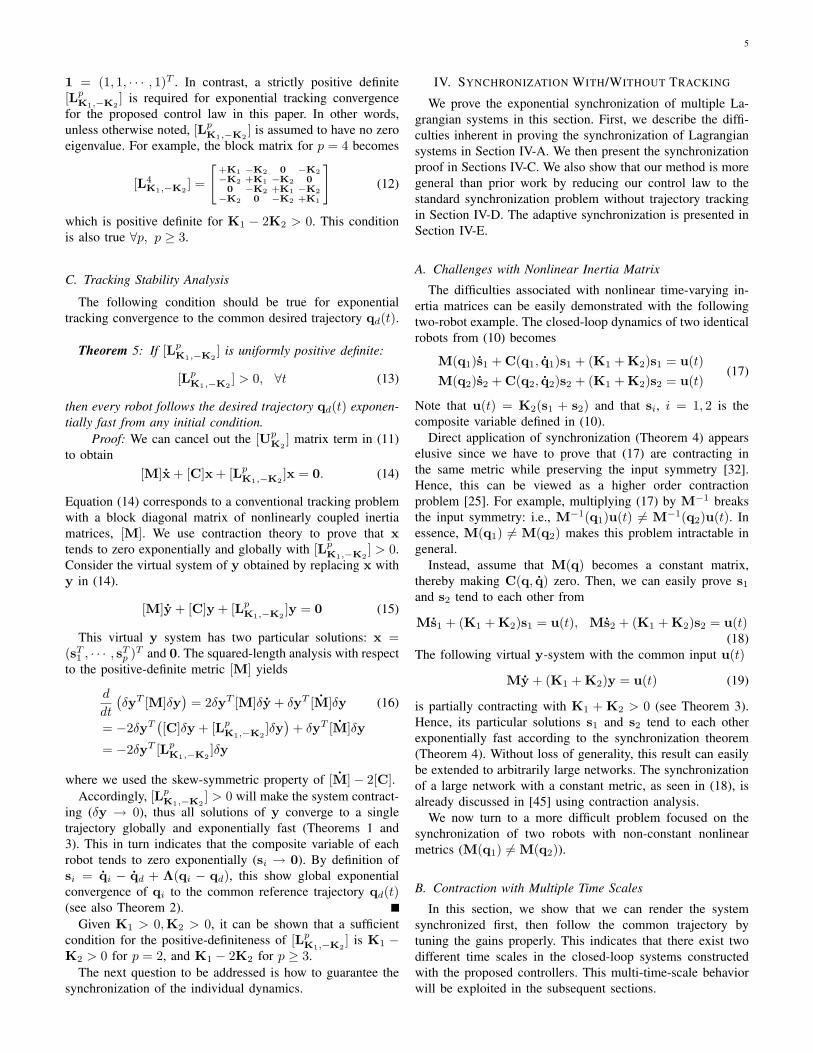
thereby ensuring that the robots synchronize faster than theyfollow the common desired trajectory.This multi timescale behavior is graphically illustrated inFigure 2. The figure depicts that s1 and s2 synchronize first,then they converge to the desired trajectory while stayingtogether. This observation motivates separation of the twodifferent time scales, namely D1 for tracking and D2 forsynchronization.
S1S2
S1=S2
S1=S2=0
synchronization
tracking
Fig. 2. Multiple timescales of synchronization (faster) and tracking (slower).The dashed line indicates the desired trajectory, and arrows indicate increasingtime. The drawing is conceptual, since strictly speaking s1 and s2 synchronizeexponentially.
C. Stability Analysis of Exponential Synchronization
Using the results from the previous sections, we present themain theorem on synchronization.
Theorem 6: Assume that the conditions in Theorem 5 aretrue, so that the individual dynamics are exponentially trackingthe common desired trajectory. A swarm of p robots synchro-nizes exponentially from any initial conditions if ∃ diagonalmatrices K1 > 0, K2 > 0, Λ > 0 such that
D2 = VTsync[L
pK1,−K2
]Vsync > 0, ∀t (25)
Proof: Consider the virtual system of y from (21):(VT [M]V
)y +
(VT [C]V
)y + [D]y = 0, (26)
This has y = VT x and y = 0 as particular solutions, whichcan be written in terms of y =
(yT
t ,yTs
)T:(
yt = [1]T xys = VT
syncx
)and
(yt = 0ys = 0
)(27)
For [D] > 0, we can show that the above virtual system iscontracting (i.e., δy→ 0 globally and exponentially). We takethe symmetric positive definite block matrix VT [M]V as ourcontraction metric.
Performing the squared-length analysis with respect to thismetric yields
d
dtδyT
(VT [M]V
)δy = −2δyT
((VT [C]V
)δy + [D]δy
)+ δyT
(VT [M]V
)δy = −2δyT [D]δy (28)
where we used the skew-symmetric property of(VT [M]V
)−
2(VT [C]V
).
The above equation can be rewritten in terms of twodifferent time scales
d
dt
(δyt
δys
)T [ [1]T [M][1] [1]T [M]Vsync
VTsync[M][1] VT
sync[M]Vsync
](δyt
δys
)(29)
= −2(δyt
δys
)T [D1 00 D2
](δyt
δys
)If D1 > 0 and D2 > 0, the combined virtual system in
(26) is contracting. In other words, δy→ 0 exponentially fast.This in turn implies that all solutions of y tend to the singletrajectory. In particular, the tracking (δyt → 0) is associatedwith D1, and synchronization (δys → 0) is associated withD2.

7
As a result, [1]T x = 1/√p(s1 + · · ·+sp) and VT
syncx from(27) tend to zero exponentially. Note that s1, · · · , sp → 0 hasalready been proven with D1 > 0 for Theorem 5, which is asufficient condition to make the sum of the composite variablesalso tend to zero (i.e., [1]T x→ 0). What is new in this sectionis the synchronization VT
syncx → 0 and its convergence ratewith D2 > 0.
It is straightforward to show that VTsyncx → 0 and Λ >
0 also hierarchically make q1, · · · ,qp synchronize globallyexponentially fast (see Theorem 2). This can be verified bythe following contracting dynamics constructed from (10)
VTsync{q}+
(VT
sync[Λ]Vsync
)VT
sync{q} = VTsyncx→ 0
(30)where {q} = (qT
1 , · · · ,qTp )T . Note that the orthonormal
vectors Vsync canceled the common input term qd + Λqd.Also, [Λ] is a block diagonal matrix of Λ > 0, thereby yieldingVT
sync[Λ][1] = 0 from
VsyncVTsync{q}+ [1][1]T {q} = {q} (31)
Consequently, VTsync{q} → 0 implies the synchronization
of the original state variable qi, i = 1, · · · , p. This also impliesthat the diagonal terms of the metric, VT
sync[M][1], tend tozero exponentially, thereby eliminating the coupling of theinertia term VT [M]V in (28–29). This completes the proofof Theorem 6.
Remark 4: We assume here that qd(t) is identical for eachmember. If qd(t) were different for each dynamics, si → sj
would imply the synchronization of qi − qj to the differenceof the desired trajectories, which would be useful to constructphase synchronization of oscillatory trajectories (e.g., see [9],[32]).
We can use Theorem 6 without finding Vsync as follows.Corollary 1: The following condition, in lieu of (25), veri-
fies Theorem 6.
[LpK1,−K2
] + [UpK2
] > 0, ∀t (32)
Proof: The block matrix [UpK2
] also has [1] as its eigen-vector. We multiply [Ksync] = [Lp
K1,−K2] + [Up
K2] by its
orthonormal eigenvectors other than [1]:
[Ksync]Vsync = [LpK1,−K2
]Vsync = VsyncD2 (33)
which shows that Vsync also represents the orthonormaleigenvectors of [Ksync] = [Lp
K1,−K2] + [Up
K2]. In other
words, D2 corresponds to the eigenvalues of [Ksync]. Theremaining eigenvalue of [Ksync] that is associated with [1] isK1 +(p−2)K2, which is greater than the tracking eigenvalueD1 = K1−2K2 for p ≥ 3. Hence, the synchronization occurswith [Lp
K1,−K2] + [U2
K2] > 0.
Theorem 6 and Corollary 1 correspond to synchronizationwith stable tracking. As shall be seen in Section V-B, multipledynamics need not be identical to achieve stable synchroniza-tion. It is useful to note that the above condition correspondsto K1 + K2 > 0 for two-robot and three-robot networks(p = 2, 3).
Remark 5: Robust Synchronization. By extending [24], wecan show that coupled contracting dynamics have the prop-erty of robustness to bounded disturbances [7]. It should be
emphasized that exponential stability of contraction analysisfacilitates such a perturbation analysis. In general, the proofof robustness with asymptotic convergence is more involved,or even leads to instability with respect to a certain class ofperturbations (see p. 350 in [17]).
In the next section, we show that a network of multiplerobots can synchronize even without stable tracking.
D. Synchronization Without a Common Reference Trajectory
We now turn into the more standard synchronization prob-lem where the tracking gain is zero (D1 = K1−2K2 = 0 forp ≥ 3), which fails the exponential tracking stability conditionin Theorem 5. In this case, the modified Laplacian [Lp
K1,−K2]
reduces to the standard weighted Laplacian whose row sum iszero. For synchronization to the weighted average of the initialconditions, we do not require the common desired trajectoryqd, and qd can simply be set to zero as follows:
qi,r = −Λqi, si = qi + Λqi (34)
In other words, our control strategy represents a moregeneralized framework for the synchronization of multipleLagrangian systems.
Theorem 7: Suppose that the individual tracking dynamicsare indifferent. Hence, the conditions in Theorem 5 are nottrue. Nevertheless, a swarm of p identical robots asymptot-ically synchronize from any initial conditions if ∃ diagonalmatrices K1 > 0, K2 such that
[LpK1,−K2
] + [UpK2
] > 0, ∀t (35)
For indifferent tracking, a common desired trajectory qd(t) isno longer required.
Proof: The combined virtual system per se is then semi-contracting (see [24]) since the squared-length analysis in (28-29) yields the negative semi-definite matrix:
V = −2(δyt
δys
)T [0 00 D2
](δyt
δys
)≤ 0 (36)
While δyt, representing the tracking dynamics, remains in afinite ball due to D1 = 0, δys tends to zero asymptoticallydue to D2 > 0. This result can be proven as follows. Notethat V = −4δyT
s D2δys. V is uniformly continuous since abounded δys from (26) leads to a bounded V . Due to V ≤ 0,the use of Barbalat’s lemma [38] verifies that V → 0 as t→∞. This implies that δys tends to zero asymptotically fast.As a result, VT
syncx tends to zero asymptotically. From thehierarchical combination discussed in (30), this also impliesVT
sync{q} → 0. This completes the proof of Theorem 7 withindifferent tracking.
This will eventually decouple the metric matrix with Λ > 0,as seen in (29), since VT
sync[M][1] tends to zero simultane-ously as VT
sync{q} → 0. As a result, when M(qi)−M(qj)is sufficiently close to zero, the convergence of δys → 0 turnsexponential.
Remark 6: Fast Inhibition. The dynamics of a large net-work with semi-contracting stability as in (36) can be instan-taneously transformed to contracting dynamics by the additionof a single inhibitory coupling link. In other words, a single
8
inhibitory link will also make δyt → 0. For instance, we canadd a single inhibitory link between two arbitrary elements aand b while we keep the rest of the elements the same: [45]
τa =M(qa)qar + C(qa, qa)qar + g(qa)− 2K2sa + K2sa−1 + K2sa+1 −K(sa + sb) (37)
τb =M(qb)qbr + C(qb, qb)qbr + g(qb)− 2K2sb + K2sb−1 + K2sb+1 −K(sa + sb)
where 2K2 is substituted for K1, and K > 0.Hence, we can straightforwardly show that [Lp
K1,−K2] is
now strictly positive definite, in contrast with the originalsemi-contracting system. As a result, the closed-loop systemis contracting, resulting in si → 0 and qi → 0 from (34).This fast inhibition is useful to rapidly destroy unwantedsynchronized oscillation of robots.
E. Adaptive Synchronization
We present the adaptive version of the proposed controllaw that adapts to the unknown parametric uncertainties ofthe robot dynamic models. Consider the following adaptivecontrol law [16], [38], [39] that has the same local couplingstructure as the proposed control law in (8):
τi = Mi(qi)qi,r + Ci(qi, qi)qi,r + gi(qi)−K1si (38)+ K2si−1 + K2si+1 = Yiai −K1si + K2si−1 + K2si+1
where si = qi − qi,r. Also, the parameter estimate ai for thei-th member is updated by the correlation integral
˙ai = −ΓYTi si (39)
where Γ is a symmetric positive definite matrix. Hence, theclosed-loop system for a network comprised of p non-identicalrobots can be written as[
[M] 00 [Γ−1]
](x{ ˙a}
)+[[C] 00 0
](x{a}
)(40)
+[[Lp
K1,−K2] −[Y]
[Y]T 0
](x{a}
)= 0
where [M] and [C] are the block diagonal matrices ofMi(qi) and Ci(qi, qi), i = 1, · · · , p, as defined in (11).The additional block diagonal matrices are defined from(39) such that [Γ−1] = diag(Γ−1,Γ−1 · · · ,Γ−1)p, [Y] =diag(Y1,Y2, · · · ,Yp). Also, x = (sT
1 , sT2 , · · · , sT
p )T , and{a} = (aT
1 , aT2 , · · · , aT
p )T where ai denotes an error of theparameter estimate such that ai = ai − ai. Note that ai is aconstant vector of the true parameter values for the i-th robot,resulting in ˙ai = ˙ai. If each robot is identical, ai = a for1 ≤ i ≤ p.
Theorem 8: The adaptive synchronization law in (38) glob-ally asymptotically synchronizes the states of multiple dynam-ics in the presence of parametric model uncertainties if thecondition (35) holds.
Proof: Similar to Section IV-C, applying the spectraltransformation, using the augmented Va = diag (V, Ipn) and
VT [LpK1,−K2
]V = [D], to (40) leads to the following virtualsystem of (yT
1 ,yT2 )T [16], [39][
VT [M]V 00 [Γ−1]
](y1
y2
)+[VT [C]V 0
0 0
](y1
y2
)(41)
+[
[D] −VT [Y][Y]T V 0
](y1
y2
)= 0
The virtual system has two particular solutions:y1 = VT x, y2 = {a}, and y1 = 0, y2 = 0The virtual length analysis indicates that (41) is semi-contracting by the negative semi-definite Jacobian with [D] >0:
dV
dt= −2
(δy1
δy2
)T [[D] 00 0
](δy1
δy2
)(42)
Using Barbalat’s lemma (see Section IV-D), it is straightfor-ward to show that δy1 tends asymptotically to zero from anyinitial condition. Also, [D] can be decomposed to the trackingand synchronization gains, and the rest of the proof followsTheorems 6 and 7. Consequently, the adaptive synchronizationlaw in (38) synchronizes the states of multiple dynamics in thepresence of parametric model uncertainties.
While the synchronization of the estimates of the physicalparameters (δy2 → 0) is not automatically guaranteed due tothe semi-contracting stability, the additional condition of thepersistency of excitation [38] leads to the convergence of a tozero. Results of the simulation are presented in Section VII-C.
F. Examples
For the case of a two-robot network, we can easily verify
z = VT x =(
[1]T
VTsync
)x =
[1√2I 1√
2I
1√2I − 1√
2I
](s1
s2
),
D1 = K1 −K2, D2 = K1 + K2 (43)
If K1 + K2 > K1 −K2 > 0, the rate of the virtual lengthV in (28) is uniformly negative definite:
V = −2(δyt
δys
)T [K1 −K2 00 K1 + K2
](δyt
δys
)< 0.
Consequently, the combined virtual system in (26) is contract-ing. As a result, s1 + s2 → 0 and s1 → s2 exponentially. Itis straightforward to show that s1 → s2 also hierarchicallymakes q1 tend to q2 exponentially as in (30).
The results hold for arbitrarily large networks as well. Forexample, a network of three robots has the following V, whosecolumns are orthonormal eigenvectors of [Lp=3
K1,−K2]:
V =[[1] Vsync
]=
[ 1√3I − 2√
6I 0
1√3I 1√
6I − 1√
2I
1√3I 1√
6I 1√
2I
]The block diagonal matrix [D] is also computed asdiag (K1 − 2K2,K1 + K2,K1 + K2).
For a four-robot network p = 4 (see Figure 1(a)), [D] =diag (K1 − 2K2,K1 + 2K2,K1,K1), and
V =12
I I 0 −√
2I
I −I −√
2I 0
I I 0√
2I
I −I√
2I 0

9
By inspecting the associated eigenvectors, we can notice thatK1 represents the synchronization gain associated with thesynchronization of diagonal members (q1 = q3,q2 = q4),while K1 +2K2 represents the synchronization gain of directcouplings (e.g., q1 = q2,q3 = q4). This is a percolationeffect discussed in [32]. The percolation effect can be exploitedin order to prove the synchronization to the large unknowninvariant set (e.g., VT
syncx = 0 from a large network) byverifying the synchronization to a known, not necessarilyinvariant, subset of the global flow-invariant set [12].
V. CONCURRENT SYNCHRONIZATION OFHETEROGENEOUS GROUPS ON UNBALANCED GRAPHS
We further generalize the proposed synchronization frame-work in the context of the concurrent synchronization of mul-tiple heterogeneous networks and leader-follower networks,which permit construction of complex network structures.
A. Inline Configuration and Uni-Directional Digraph
We can also consider the inline configuration shown inFig. 1(f), when maintaining a ring structure is not feasiblepossibly due to communication problems.
Corollary 2: All the previous theorems hold for networkstructures on inline configuration, if the first and last robotadjust the proposed control law in (8) as
τi = M(qi)qi,r+C(qi, qi)qi,r+g(qi)−(K1−K2)si+K2sj
(44)where i = 1 or i = p, and j is the index for its sole neighbor.
Proof: We can show that the modified Laplacian[Lp
K1,−K2] constructed from both (8) and (44) is symmetric
and still has [1] as its eigenvector associated its eigenvalueD1 = K1 − 2K2. Then the proofs of the theorems easilyfollow.
Let us now consider the generalized control law in (7),which permits regular digraphs, as shown in Figures 1(c) and(d). The modified Laplacian matrix [Lp
K1,−K2] defined from
(7) might have two or more than three nonzero elements ineach row. Further, it is no longer symmetric.
Corollary 3: All the previous theorems are valid for regulargraphs with uni-directional couplings or both uni-directionaland bi-directional couplings.
Proof: It is straightforward to verify that the sym-metric matrix [Lp
K1,−K2] + [Lp
K1,−K2]T has the same
number of nonzero elements at each row (i.e., reg-ular). Hence, we can conclude that all the previousproofs still hold. For example, the synchronization occurswhen VT
sync
([Lp
K1,−K2] + [Lp
K1,−K2]T)
Vsync > 0 while
[1]T([Lp
K1,−K2] + [Lp
K1,−K2]T)
[1] determines the stabilityand convergence rate of the trajectory tracking.
B. Synchronization of Heterogeneous Robots
Consider the proposed control law for a network comprisedof heterogeneous dynamics as follows:
τi = Mi(qi)qi,r + Ci(qi, qi)qi,r + gi(qi) (45)−K1(qi − qi,r) + K2(qi−1 − qi−1,r) + K2(qi+1 − qi+1,r)
Leader
2nd Network
1st
Network
Fig. 3. Concurrent synchronization between two different groups. The desiredtrajectory inputs are denoted by the dashed-lines whereas the solid linesindicate mutual diffusive couplings. The independent leader sends the samedesired trajectory input to the first network group. If we view the dashed-linesas edges of the graph, the network is on an unbalanced graph.
where Mi, Ci, and gi(qi) represent the i-th robot dynamics,which can be different from robot to robot. Each robot has thesame number of configuration variables (qi ∈ Rn).
Corollary 4: The proposed tracking and synchronizationcontrol law in (8) can easily be applied to a network consistingof heterogeneous robots in (2) if the stable tracking conditionin Theorem 6 is true.
Proof: The M and C matrix notations used in theprevious sections can be interpreted as M(q1) → M1(q1)and M(q2) → M2(q2) with M1(·) 6= M2(·) (the samefor the C matrices). Hence, the assumption of non-identicaldynamics does not alter the proof of exponential tracking inTheorem 5 and stable synchronization in Theorem 6. However,the synchronization with indifferent tracking (Theorem 7) isno longer true for non-identical robots since VT
syncx = 0 isnot a flow-invariant manifold, and q1 = q2 does not cancelthe off-diagonal terms 1/2 [M1(q1)−M2(q2)] in the metricmatrix VT [M]V.
C. Concurrent Synchronization of Heterogeneous Groups
We present a new method of achieving the concurrentsynchronization of multiple heterogeneous networks in thissection. Such a method can be used to apply the mainresults in the previous sections to more complex networks, asshown in Figure 1(e). The networks in the figure are neitherregular nor balanced due to the reference input couplings.In [32], concurrent synchronization is defined as a regimewhere the ensemble of dynamical elements is divided intomultiple groups of fully synchronized elements, but elementsfrom different groups are not necessarily synchronized and canexhibit entirely different dynamics.
As discussed in the previous sections, we pay particularattention to the fact that there exist two different time scalesof the proposed synchronization tracking control law. Inparticular, one rate is associated with the trajectory tracking(D1), while the other represents the convergence rate of thesynchronization (D2). This implies that there are two differentinputs to the system, namely, the common reference trajectoryqd(t) and the diffusive couplings with the adjacent members.Accordingly, we exploit a desired trajectory qd(t) to createmultiple combinations of different dynamics groups.

10
For instance, Figure 3 represents the concurrent synchro-nization of two different dynamic networks. The first network,consisting of four heterogeneous robots, has the diffusivecoupling structure proposed by the tracking control law in (8).The independent leader sends a desired trajectory commandqd(t) to each member of the first network. Note that thedimension of the leader dynamics need not be equal to thatof the first network, since a signal from the leader can bepre-conditioned. With an appropriate selection of gains, eachdynamics in the first network synchronize while exponentiallyfollowing the leader. Therefore, the proposed scheme can beinterpreted in the context of the leader-follower problem ([15],[21], [47]).
The second network consists of three heterogeneous dynam-ics, also different from those of the first group. Each elementreceives a different desired trajectory input from the adjacentelement of the first network. Again, the desired trajectory inputfor the second group can be pre-conditioned from the firstnetwork, resulting in
q2d(t) = f(q1, t) (46)
where q1 is the state vector of the member in the first networkthat sends in the desired command and f is a differentiablenonlinear function of q1. As a result, the dynamics of the twonetworks can be entirely different (i.e., q1 ∈ Rm, q2 ∈ Rn,and m 6= n). Note that q2d, needed for the proposed controllaw in (7), can be obtained from a nonlinear observer [38].The concurrent synchronization between the first and secondnetworks can be proven as follows.
Corollary 5: Consider the network structures that are un-balanced (i.e., the in-degrees are not equal to the out-degrees)due to the directional reference input connections amongthe regular balanced graphs, shown as the dashed lines inFigures 1(e) and 3. The robots on such graphs globallyexponentially synchronize if the individual groups synchronizefrom Theorems 5 and 6.
Proof: For the example shown in Figure 3, once thefirst network synchronizes, the second network also ends upreceiving the same desired trajectory to follow, while theyinteract to synchronize exponentially fast. Accordingly, wecan achieve concurrent synchronization between two differentnetwork groups. The proof of Theorem 6 holds until (30),where now the desired trajectory inputs are different for eachrobot. Then, we can conclude that the robots in the secondnetwork synchronize, if the desired reference inputs q2d,i,1 ≤ i ≤ p, sent from the first network, synchronize:
VTsync{q2}+
(VT
sync[Λ]Vsync
)VT
sync{q2} (47)
−(VT
sync[rT1 , · · · , rT
p ]T → 0)
= VTsyncx2 → 0
where ri = q2d,i + Λq2d,i, and x2 is the vector of thecomposite variables (si) of the second network. If the firstnetwork synchronizes, the reference trajectory term vanishes(VT
sync[rT1 , · · · , rT
p ]T → 0), thereby ensuring the synchroniza-tion of the second network (i.e., VT
sync{q2} → 0). This can beextended to arbitrarily large groups of synchronized dynamicsby appropriately assigning the desired trajectory inputs andthe diffusive couplings.
Remark 7: The previous example in Figure 3 and Corol-lary 5 can be interpreted in terms of feedback hierarchies(see Theorem 2). The first network in the figure providesfeedforward commands to the second network, but does notreceive any command from the second network. Note thatthe dynamics at each level can be very different, in order toconstruct a dynamic concurrent combination of heterogeneousnetworks. Since the feedforward inputs can be appropriatelyscaled and conditioned, the dimensions between hierarchicallayers can also be very different. For example, the dynamicshigher in the hierarchy need not be oscillators, but couldbe systems with multiple equilibria (e.g., x = −∇V , withlocal minima in V [39]), with synchronization correspond-ing to convergence toward a common minimum. Concurrentsynchronization discussed in this section can be exploited toconstruct a large complex network consisting of heterogeneousdynamics such as robots, ground vehicles, and unmannedaerial vehicles.
VI. EXTENSIONS
Let us further extend the proposed control law.
A. Synchronization of Robots Using Linear PD Control
One may consider the following Proportional and Derivative(PD) coupling control law for two identical robots from (2)with p = 2,
τ1 = −K1(q1 + Λq1) + K2(q2 + Λq2)τ2 = −K1(q2 + Λq2) + K2(q1 + Λq1)
(48)
where qi = qi − qd and the bounded reference position qd
has zero velocity such that ˙qi = qi.For simplicity, the gravity term in (2) is assumed to be zero orcanceled by a feed-forward control law. Then, the closed-loopdynamics satisfy
M(q1)q1 + C(q1, q1)q1 + Kq1 + KΛq1 = u(t)M(q2)q2 + C(q2, q2)q2 + Kq2 + KΛq2 = u(t)
(49)
where K = K1 + K2 and u(t) = K2(q1 + q2) + K2Λ(q1 +q2).
Similar to Section IV-C, we can perform a spectral decom-position:(VT [M]V
)VT x +
(VT [C]V
)VT x (50)
+(VT [Lp
K1,−K2]V)
VT x +(VT [Lp
K1Λ,−K2Λ]V)
VT x = 0
Using the following Lyapunov function, it is straightforwardto show that this PD coupling control law drives the systemto the desired rest state qd globally and asymptotically whiletending to the synchronized flow-invariant manifold:
V =12
(qp
qm
)T [M1+M22
M1−M22
M1−M22
M1+M22
](qp
qm
)(51)
+12
(qp
qm
)T [(K1 −K2)Λ 00 (K1 + K2)Λ
](qp
qm
)

11
where M1 = M(q1), M2 = M(q2), VT x =(
qp
qm
)=
1√2
(q1 + q2
q1 − q2
), qp = 1√
2(q1 + q2).
The rate of V can be computed as
dV
dt= −
(qp
qm
)T [K1 −K2 00 K1 + K2
](qp
qm
)≤ 0 (52)
which implies that V is negative semi-definite with K1+K2 >0 and K1 −K2 > 0.
By invoking LaSalle’s invariant set theorem [38], we canconclude that qp, qp, qm, and qm tend to zero with globaland asymptotic convergence. This implies that q1 and q2 willfollow qd while q1 and q2 synchronize asymptotically fromany initial condition. This can be extended to arbitrarily largenetworks as shown in Figure 1.
Note that if Λ = 0, the PD coupling control law in (48)reduces to velocity coupling
τ1 = −K1q1 + K2q2, τ2 = −K1q2 + K2q1 (53)
This velocity coupling control can also be derived from theexponential tracking control law in (8) by setting qd = 0,qd = 0, and Λ = 0. Therefore, the proof of the linear PDsynchronization with Λ = 0 is the same as Section IV-Cwhereas the convergence rate is now exponential comparedwith the asymptotic convergence of the PD control. On theother hand, we can find that positions do not synchronize inthe absence of the gravity term even though the velocitiessynchronize exponentially fast.
B. Synchronization with Limited Communication Bandwidth
We now consider multiple dynamics with partially coupledjoints (or partially coupled variables). For example, we canassume that only the lower joint is coupled in a two-robotsystem having two joint variables with q = (x1, x2)T for(i = 1, j = 2) or (i = 2, j = 1):
τi = M(qi)qi,r + C(qi, qi)qi,r + g(qi)−K1si
+ K2
( ˙x1
0
)qj
+ K2Λ(x1
0
)qj
(54)
Nevertheless, Theorems 5 and 6 are true with diagonalmatrices, K1, K2 and Λ, which can be verified by writingthe closed-loop system as in (17):
M(q1)s1 + C(q1, q1)s1 + (K1 + K2P)s1 = u(t) (55)M(q2)s2 + C(q2, q2)s2 + (K1 + K2P)s2 = u(t)
u(t) = K2P(s1 + s2), P = diag(1, 0)
It is straightforward to prove that Theorems 5 and 6 stillhold. This is because (K1 + K2P) and (K1 − K2P) arestill uniformly positive definite, enabling exponential synchro-nization and exponential convergence to the desired trajectory,respectively. Hence, we did not break any assumption in theproof of Theorem 6. This partial-state coupling also works forthe semi-contracting case with (34), as presented in SectionIV-D. While the coupled variables synchronize to the weightedaverage of the initial conditions, the uncoupled variablessynchronize to zero.
C. Synchronization with Time-Delays
The results may be extended to time-delayed couplings (seealso [4]). Consider for instance the two-robot dynamics (17),which becomes
M(q1)s1 + C(q1, q1)s1 + (K1 −K2)s1 = τ21
M(q2)s2 + C(q2, q2)s2 + (K1 −K2)s2 = τ12
τ21 = K2(s2(t− T )− s1(t)) (56)τ12 = K2(s1(t− T )− s2(t))
where the constant T > 0 denotes the communication delaybetween the two robots, and s(t − T ) = q(t − T ) + Λq(t −T )− (qd(t) + Λqd(t)).
Theorem 9: The robots in (56) synchronize globally asymp-totically ∀T > 0 under the assumptions of Theorem 6.
Proof: Similar to [40], [46], consider the differentiallength
V = δzT(VT [M]V
)δz +
∫ t
t−T
δzT (ε)[
K2 00 K2
]δz(ε)dε
(57)Using (56) shows that V is negative semi-definite,
V =− 2δzT[
K1−K2 00 K1−K2
]δz (58)
− δτT21K
−12 δτ21 − δτT
12K−12 δτ12
Note that K1 + K2 > K1 −K2 > 0 implies K2 > 0.Also, V is bounded. By Barbalat’s lemma, V tends to
zero globally asymptotically, which in turn implies δz →0, δτ21 → 0, δτ12 → 0. Hence, the solutions converge to asingle trajectory asymptotically. Since s1(t− T ) = s2(t− T )is a particular solution of (56), q1(t) and q2(t) globallyasymptotically synchronize regardless of T .
D. A Perspective on Model Reduction by Synchronization
Another benefit of exponential synchronization is its impli-cation for model reduction [8]. Exponential synchronization ofmultiple nonlinear dynamics allows us to reduce the dimen-sionality of the stability analysis of a large network. As notedearlier, the synchronization rate (D2) is faster than the trackingrate (D1). Assuming that the dynamics are synchronized, theaugmented dynamics in (14) reduces to
M(q)s + C(q, q)s + (K1 − 2K2)s = 0 (59)
where q = q1 = · · · = qp, and D1 = K1 − 2K2 is replacedby K1 −K2 for p = 2.This implies that once components of a network are shownto synchronize, we can regard them as a single dynamics ofreduced dimension, which simplifies any additional stabilityor perturbation analysis.
VII. SIMULATION RESULTS
A. Tracking Synchronization of Four Robots
Even though the local coupling structure of (7) and (8) hasbeen emphasized, the difference from all-to-all coupling is notevident in a network comprised of less than four members(p ≤ 3). To illustrate the effectiveness of the proposed schemefor a robot network with p ≥ 4, a network of four identical

12
0 1 2 3 4 5 6 7 8.5
1
.5
0
.5
1
.5
2
s[m]
Robot 1
Robot 2
Robot 3
Robot 4
(a) Simulation result.
0 5 10 15 20 25 30 35 40
−0.4
−0.2
0
0.2
0.4
s [m
]
Tracking errors of four−robot network
0 5 10 15 20 25 30 35−1.5
−1
−0.5
0
Join
t 1 [r
ad]
Robot1Robot2Robot3Robot4
0 5 10 15 20 25 30 35 40
0
0.5
1
1.5
2
time [s]
Join
t 2 [r
ad]
(b) Tracking error of each robot
Fig. 4. Synchronization of a four-robot network
3-DOF robots is considered here (see Fig 1(a)). The dynamicsmodeling of the 3-DOF robot is based upon the double invertedpendulum robot on a cart (see Fig. 4(a)), and each joint isassumed to be frictionless. The physical parameters of eachrobot are given in [7].
The simulation result is presented in Figure 4. The fouridentical robots, initially at some arbitrary initial condi-tions, are driven to synchronize as well as to track thetime-varying desired trajectory: sd(t) = 0.2t, θ1d(t) =cos(0.02πt), θ2d(t) = π/4(1− cos(0.08πt)). For the controlgains in the control law (8), we used K1 = 5I, K2 = 2I, andΛ = 5I. According to Theorems 5 and 6, the tracking gainK1 − 2K2 is smaller than the corresponding synchronizationgains K1+2K2 and K1. Figure 4(b) shows the tracking errorsof the four robots. We can see that the robots synchronizeexponentially fast from arbitrary initial conditions, and thissynchronization occurs faster than the exponential convergenceof tracking errors. Such a result can be useful to rapidlyachieve a collective motion of multiple robots in the presenceof external disturbances. If K1 = 2K2 instead, we can easilyshow that the robots synchronize with global exponentialconvergence, although the tracking errors will not tend to zero.
B. Simulation of Concurrent Synchronization for Ten Robots
Let us consider three heterogeneous networks connectedby feedback hierarchies shown in Fig. 5(a). If we view the
5
3
21
6 4
9
10
8
7
2
1
3
(a) Three networks connected by feedback hierarchies.
0 5 10 15 20 25 30 35 40−0.6−0.4−0.2
00.20.4
s [m
]
Tracking errors of ten−robot network
0 5 10 15 20 25 30 35 40−1.5
−1
−0.50
Join
t 1 [r
ad]
0 5 10 15 20 25 30 35 40
0
1
2
time [s]
Join
t 2 [r
ad]
(b) Tracking error of each robot
Fig. 5. Synchronization of ten robots on three heterogeneous networks
reference trajectory inputs (dashed lines in the figure) asedges of the graph, as discussed in Section V, this graph isunbalanced. The first network (robot 1 through 4) is identicalto the network of four 3-DOF robots in the previous section.All the physical parameters of the second network (robot 5through 7) are twice larger than those of the first networkwhile those of the third network are 1.5 times larger. Also,note that the third network is on an inline configuration byconnecting the second feedback gain K2 of the control law in(8) back to itself. All the previous theorems still hold for suchan inline configuration (see Corollary 2). As seen in Fig. 5(b),the first, second, and third network individually synchronizerobots within each network from arbitrary initial conditions.The first and second network also follow the reference trajec-tory command from the adjacent members. For the referencetrajectory commands, we assume that we can send the positionand velocity values (qd, qd). Then, qd is estimated by a highpass filter. Eventually, all the robots exponentially synchronizeand then follow the desired trajectory staying together. Thisconcurrent synchronization can be used to construct a complexand large-scale dynamic network consisting of an arbitrarynumber of heterogeneous robots and networks.
C. Simulation of Adaptive Synchronization
We assess the effectiveness of the proposed adaptive syn-chronization control law presented in Section IV-E. Considera two-robot network, comprised of the two-link manipulatorrobots given in page 396 of [38]. The desired trajectory forthe first joint is θ1d(t) = sinπt and for the second joint isθ2d(t) = 2(1 − cos 0.6πt). The initial parameter estimatesfor both robots are defined as a(0) = (3, 1, 1, 1)T , andΓ = diag(0.03, 0.05, 0.1, 0.3). Figure 6(a) shows the synchro-nization of the two robots with stable tracking by K1 = 20I,K2 = 15I, and Λ = 10I. Hence, the synchronization gain

13
K1 + K2 is larger than the tracking gain K1 − K2. Notethat the synchronization of the tracking errors implies thesynchronization of the state variables (i.e., joint 1 and joint2). As discussed before, the synchronization occurs faster thanthe tracking. This simulation result indicates that the proposedadaptive control law can be used to synchronize motions ofrobots with unknown physical parameters.
In contrast, Figure 6(b) shows the synchronization withindifferent tracking by the gains of K1 = K2 = 20I andΛ = 10I. The tracking dynamics then have zero gain (indif-ferent). So the two robots synchronize asymptotically, whilethe tracking errors remain within a finite ball. In both cases(Figs. 6(a) and (b)), the proposed adaptive control law ensuresneither the asymptotic convergence nor the synchronization ofthe physical parameter estimates ai, unless the persistency ofexcitation condition is met. Nevertheless, the robots synchro-nize asymptotically from any initial condition in the presenceof such parametric uncertainty. This adaptive version makesthe proposed synchronization framework more practical. Itshould also be obvious to readers that the proposed control lawcan be straightforwardly extended to robust adaptive controlschemes based on sliding control [38].
VIII. CONCLUSIONS
We have presented the new synchronization tracking controllaw that can be directly applied to cooperative control ofmulti-robot systems and oscillation synchronization in roboticmanipulation and locomotion. We have also shown that com-plex dynamic networks can be constructed by exploitingconcurrent synchronization such that multiple groups of fullysynchronized elements coexist. The proposed decentralizedcontrol law, which requires only local coupling feedback forglobal exponential convergence, eliminates both the all-to-allcoupling and the feedback of the acceleration terms, therebyreducing communication burdens and complexity. Further-more, in contrast with prior work which used simple singleor double integrator models, the proposed method permitshighly nonlinear systems. Providing exact nonlinear stabilityresults constitutes one of the main contributions of this paper;global and exponential stability of the closed-loop system hasbeen derived by using contraction theory. Contraction analysis,overcoming a local result of Lyapunov’s indirect method,yields global results based on differential stability analysis.While we have focused on the mutual synchronization prob-lem where synchronization and trajectory tracking take placesimultaneously, the proposed method has also been shown tobe a generalization of the average consensus problem that doesnot address trajectory tracking. It has been emphasized thatthere exist multiple time scales in the closed-loop systems:the faster convergence rates represents the transient boundarylayer dynamics of synchronization while the slower rate deter-mines how fast the synchronized systems track the commonreference trajectory. Exponential synchronization with a fasterconvergence rate enables reduction of multiple dynamics intoa simpler form, thereby simplifying the stability analysis.
Simulation results show the effectiveness of the proposedcontrol strategy. The proposed bi-directional coupling has
0 5 10 15 20 25
−1
−0.5
0
0.5
time[s]
Tra
ckin
g E
rror
[rad
]
Synchronization with Asymptotic Tracking
0 5 10 15 20 25−6
−4
−2
0
2
4
time[s]
Par
amet
er E
stim
ates
#1:θ1 #1:θ2 #2:θ1 #2:θ2
#1: a1 a2 a3 a4 #2:a1 a2 a3 a4
(a) with asymptotically stable tracking
0 5 10 15 20 25
−1
−0.5
0
0.5
time[s]
Tra
ckin
g E
rror
[rad
]
Synchronization with Indifferent Tracking
0 5 10 15 20 25−6
−4
−2
0
2
4
6
time[s]
Par
amet
er E
stim
ates
#1:θ1 #1:θ2 #2:θ1 #2:θ2
#1: a1 a2 a3 a4 #2:a1 a2 a3 a4
(b) with indifferent tracking
Fig. 6. Adaptive synchronization of two two-link manipulator robots
also been generalized to permit partial-state coupling anduni-directional coupling. Further extensions to proportional-derivative coupling, adaptive synchronization, time-varyingnetwork topology, and concurrent synchronization of multipleheterogeneous networks on unbalanced graphs exemplify thebenefit of the proposed approach based on contraction theory.
ACKNOWLEDGEMENTS
This paper benefited from constructive comments from theassociate editor, anonymous reviewers, Dr. Keehong Seo, andProf. David W. Miller at MIT.
REFERENCES
[1] S. Arimoto, F. Miyasaki, H. G. Lee, and S. Kawamura, “Revival ofLyapunovs direct method in robot control and design,” in Proc. AmericanControl Conf., Atlanta, GA, June 1988, pp. 1764–1769.
[2] S. Arimoto, Control Theory of Nonlinear Mechanical Systems: APassivity-based and circuit-theoretic approach, Oxford University Press,Oxford, UK, 1996.
[3] N. Chopra and M. W. Spong, “On synchronization of networked passivesystems with time delays and application to bilateral teleoperation,”Proceedings of the SCIE Annual Conference, Okayama, Japan, August8-10, 2005, pp. 3424-3429.
14
[4] N. Chopra and M. W. Spong, “Passivity-based control of multi-agentsystems,” in Advances in Robot Control: From everyday physics tohuman-like movements, Sadao Kawamura and Mikhail Svinin, Editors,Springer-Verlag, Berlin, 2006, pp. 107–134.
[5] F. Chung, Spectral Graph Theory, Number 92 in CBMS RegionalConference Series in Mathematics, American Mathematical Society,1997.
[6] S.-J. Chung and J.-J. E. Slotine, “Cooperative robot control and synchro-nization of Lagrangian systems,” Proc. 46th IEEE Conf. on Decision andControl, New Orleans, LA, Dec. 2007, pp. 2504–2509.
[7] S.-J. Chung, “Nonlinear control and synchronization of multiple La-grangian systems with application to tethered formation flight space-craft,” Doctor of Science Thesis, Dept. of Aeronautics and Astronautics,Massachusetts Inst. of Technology, Cambridge MA, 2007.
[8] S.-J. Chung, J.-J. E. Slotine, and D. W. Miller, “Nonlinear modelreduction and decentralized control of tethered formation flight,” Journalof Guidance, Control, and Dynamics, Vol. 30, No. 2, pp. 390–400,March–April 2007.
[9] S.-J. Chung, U. Ahsun, and J.-J. E. Slotine, “Application of synchro-nization to formation flying spacecraft: Lagrangian approach,” acceptedfor publication, Journal of Guidance, Control and Dynamics, to bepublished.
[10] B. P. Demidovich, “Dissipativity of a nonlinear system of differentialequations,” ser. matematika mehanika, part I N.6, pp. 19–27; part IIN.1, pp.3–8 Vestnik Moscow State University, 1962.
[11] R. Fierro, P. Song, A. Das, and V. Kumar, “Cooperative control of robotformations,” in Cooperative Control and Optimization: Series on AppliedOptimization, Kluwer Academic Press, pp. 79–93, 2002.
[12] L. Gerard and J.-J. E. Slotine, “Neuronal networks and controlledsymmetries, a generic framework,” arXiv:q-bio/0612049v2 [q-bio.NC].
[13] P. Hartmann, Ordinary Differential Equations John Wiley & Sons, NewYork, 1964.
[14] I.-A. F. Ihle, M. Arcak, and T. I. fossen, “Passivity-based designs forsynchronized path-following,” Automatica, Vol. 43, No. 9, pp. 1508–1518, 2007.
[15] A. Jadbabaie, J. Lin, and A. S. Morse, “Coordination of groups ofmobile autonomous agents using nearest neighbor rules,” IEEE Trans.on Automatic Control, Vol. 48, No. 6, pp. 988–1001, June 2003.
[16] J. Jouffroy and J.-J. E. Slotine, “Methodological remarks on contractiontheory,” IEEE Conf. on Decision and Control, Atlantis, Paradise Island,Bahamas, 2004.
[17] H. K. Khalil, Nonlinear Systems, 3rd Ed.,Prentice Hall, Upper SaddleRiver, NJ, 2002, pp. 339–350.
[18] K. Krstic, I. Kanellakopoulos, and P. Kokotovic, Nonlinear and Adaptivecontrol Design, John Wiley and Sons, New York, NY, 1995, pp. 21–29.
[19] D. Lee and P. Y. Li, “Formation and maneuver control of multiplespacecraft,” Proc. of the 2003 American Control Conf., Vol. 1, June2003, pp. 278–283.
[20] D. Lee and M. W. Spong, “Stable flocking of multiple inertial agentson balanced graph,” Proc. of the 2006 American Control Conf., Vol. 52,June 2006, pp. 1469–1475.
[21] N. E. Leonard and E. Fiorelli, “Virtual leaders, artificial potentials andcoordinated control of groups,” Proc. 40th IEEE Conf. on Decision andControl, 2001, pp. 2968–2973.
[22] D. C. Lewis, “Metric properties of differential equations,” AmericanJournal of Mathematics, Vol. 71, pp. 294–312, 1949.
[23] Z. Lin, M. Broucke, and B. Francis, “Local control strategies for groupsof mobile autonomous agents,” IEEE Trans. on Automatic Control, Vol.49, No. 4, pp. 622–629, Apr. 2004.
[24] W. Lohmiller and J.-J. E. Slotine, “On contraction analysis for nonlinearsystems,” Automatica, Vol. 34, No. 6, pp. 683-696, 1998.
[25] W. Lohmiller and J.-J. E. Slotine, “High-order nonlinear contractionanalysis,” MIT Nonlinear Systems Laboratory (NSL) Report, NSL-050901.
[26] M. Mesbahi and F. Y. Hadaegh, ”Formation flying of multiple spacecraftvia graphs, matrix inequalities, and switching,” Journal of Guidance,Control, and Dynamics, Vol. 24, No. 2, pp. 369–377, 2001.
[27] G. Niemeyer and J.-J. E. Slotine, “Telemanipulation with time delays,”Int. J. of Robotics Research, Vol. 23, No. 9, pp. 873–890, 2004.
[28] R. Olfati-Saber and R. M. Murray, “Consensus problems in networksof agents with switching topology and time-delays,” IEEE Trans. onAutomatic Control, Vol. 49, No. 9, pp. 1520–1533, Sep. 2004.
[29] P. Ogren, M. Egerstedt, and X. Hu, “A control Lyapunov functionapproach to multiagent coordination,” IEEE Trans. on Robotics andAutomation, Vol. 18, No. 5, pp. 847–851, Oct. 2002.
[30] P. Ogren, E. Fiorelli, and N. E. Leonard, “Cooperative control ofmobile sensor networks: adaptive gradient climbing in a distributedenvironment,” IEEE Trans. on Automatic Control, Vol. 49, No. 8, pp.1292–1302, 2004.
[31] D. A. Paley, N. E. Leonard, R. Sepulchre, D. Grunbaum, and J. K.Parrish, “Oscillator models and collective motion: spatial patterns in thedynamics of engineered and biological networks,” IEEE Control SystemsMagazine, Vol. 27, No. 4, pp. 89–105, August, 2007
[32] Q.-C. Pham and J.-J. E. Slotine, “Stable concurrent synchronization indynamic system networks,” Neural Networks, Vol. 20, No. 1, pp. 62–77,2007.
[33] A. Pitti, M. Lungarella, and Y. Kuniyoshi, “Synchronization: adaptivemechanism linking internal and external dynamics,” Proc. of the 6th Int.Workshop on Epigenetic Robotics, Paris, France, Sept. 2006.
[34] W. Ren, “Multi-vehicle consensus with a time-varying reference state,”Systems & Control Letters, Vol. 56, No. 7-8, pp. 474–483, July, 2007.
[35] W. Ren, R. W. Beard, and E. Atkins, “Information consensus inmultivehicle cooperative control: collective group behavior through localinteraction,” IEEE Control Systems Magazine, Vol. 27, No. 2, pp. 71–82,April, 2007.
[36] A. Rodriguez-Angeles and H. Nijmeijer, “Mutual synchronization ofrobots via estimated sate feedback: a cooperative approach,” IEEE Trans.on Control Systems Technology, Vol. 12, No. 4, pp. 542–554, July 2004.
[37] K. Seo, S.-J. Chung, and J.-J. E. Slotine, “CPG-based control of a turtle-like underwater vehicle,” Proc. of the Robotics: Science and Systems(RSS), Switzerland, June 2008.
[38] J.-J. E. Slotine and W. Li, Applied Nonlinear Control, Prentice Hall,.New Jersey, 1991.
[39] J.-J. E. Slotine, “Modular stability tools for distributed computation andcontrol,” Int. J. Adaptive Control and Signal Processing, Vol. 17, No.6, pp. 397–416, 2003.
[40] J.-J. E. Slotine and W. Lohmiller, “Modularity, evolution, and the bindingproblem: a view from stability theory,” Neural Networks, Vol. 14, No.2, pp. 137–145, 2001.
[41] J.-J. E. Slotine, W. Wang, and K. El Rifai, “Synchronization in networksof nonlinearly coupled continuous and hybrid oscillators,” Proc. ofthe 6th International Symposium on Mathematical Theory of Networksand Systems (MTNS 2004), Katholieke Universiteit Leuven, Leuven,Netherlands, Jul. 5–9, 2004.
[42] G. Strang, Introduction to Applied Mathematics, Wellesley-CambridgePress, Wellesey, MA, 1986.
[43] D. Sun and J. K. Mills, “Adaptive synchronized control for coordinationof multi-robot assembly tasks,” IEEE Trans. on Robotics and Automa-tion, Vol. 18, No. 4, pp 498–510, Aug. 2002.
[44] D. Sun, L. Ren, J. K. Mills, and C. Wang, “A synchronous trackingcontrol of parallel manipulators using cross-coupling approach,” Int. J.of Robotics Research, Vol. 25, No. 11, pp. 1137–1147, Nov. 2006.
[45] W. Wang and J.-J. E. Slotine, “On partial contraction analysis forcoupled nonlinear oscillators,” Biological Cybernetics, Vol. 92, No. 1,pp. 38-53, 2005.
[46] W. Wang and J.-J. E. Slotine, “Contraction analysis of time-delayedcommunications and group cooperation,” IEEE Trans. on AutomaticControl, Vol. 51, No. 4, pp. 712–717, Apr. 2006.
[47] W. Wang and J.-J. E. Slotine, “A theoretical study of different leaderroles in networks,” IEEE Trans. on Automatic Control, Vol. 51, No. 7,pp. 1156–1161, 2006.