coplanar air launch with gravity-turn launch trajectories
TRANSCRIPT

AI
AP
COPLANAR AIR LAUNCH WITH GRAVITY-TURN
LAUNCH TRAJECTORIES
THESIS
David W. Callaway, 1st Lieutenant, USAF
AFIT/GAE/ENY/04-M04
DEPARTMENT OF THE AIR FORCE AIR UNIVERSITY
R FORCE INSTITUTE OF TECHNOLOGY
Wright-Patterson Air Force Base, Ohio
PROVED FOR PUBLIC RELEASE; DISTRIBUTION UNLIMITED.

The views expressed in this thesis are those of the author and do not reflect the official
policy or position of the United States Air Force, Department of Defense, or the United
States Government.

AFIT/GAE/ENY/04-M04
COPLANAR AIR LAUNCH WITH GRAVITY-TURN
LAUNCH TRAJECTORIES
THESIS
Presented to the Faculty
Department of Aeronautics and Astronautics
Graduate School of Engineering and Management
Air Force Institute of Technology
Air University
Air Education and Training Command
In Partial Fulfillment of the Requirements for the
Degree of Master of Science in Aeronautical Engineeering
David W. Callaway, B.S.
First Lieutenant, USAF
March 2004
APPROVED FOR PUBLIC RELEASE; DISTRIBUTION UNLIMITED
AFIT/GAE/ENY/04-M04
COPLANAR AIR LAUNCH WITH GRAVITY-TURN
LAUNCH TRAJECTORIES
David W. Callaway, B.S. First Lieutenant, USAF
Approved:
//SIGNED/ _________________________________ ____________ Dr. William E. Wiesel date Thesis Advisor
//SIGNED/ _________________________________ ____________ Dr. Steven G. Tragesser date Committee Member
//SIGNED/ _________________________________ ____________ Dr. Donald L. Kunz date Committee Member

AFIT/GAE/ENY/04-M04
Abstract
The purpose of this study was to determine the feasibility of launching a vehicle
based on the Boeing AirLaunch System in a coplanar, direct to rendezvous trajectory
with gravity-turn. The focus of the research was to model the launch trajectory and
determine the ability to reach different coplanar orbits. The launch trajectory was
modeled using two-dimensional equations of motion and a boundary value problem was
posed and solved for the gravity-turn trajectory. Trajectories were then created in an
attempt to reach different altitudes through coasting and transfer orbits. Finally a specific
orbital altitude was chosen and the trajectories were analyzed to find the most efficient
route to the target orbit for fuel and time.
iv

Acknowledgements
I would like to thank my thesis advisor, Dr. William Wiesel, for his time, patience
and support in this research effort. By sharing his knowledge, humor, and interests with
me, he made the thesis process much more enjoyable. I would like to thank my fellow
students, Dennis McNabb, Chris Blackwell, and Brian Lutz. Without their help in some
way or form, I would not have reached this point. Finally, I’d like to thank my family
and closest friends (there are too many to name here); but without whose support,
friendships and guidance, I would not be where I am today.
v

Table of Contents
Page
Abstract ............................................................................................................................ iv
Acknowledgements ............................................................................................................v
LIST OF FIGURES....................................................................................................... viii
LIST OF TABLES........................................................................................................... ix
I. INTRODUCTION..........................................................................................................1
1.1 Motivation............................................................................................................1
1.2 Overview....................................................................................................................2
1.3 Vehicle Background ..................................................................................................3
II. MODELING THE TRAJECTORY...........................................................................6
2.1 Literature Search........................................................................................................6
2.2 Reference Frames.................................................................................................6
2.3 State Variables and Equations of Motion ..................................................................9
2.3 Hohmann Transfer .............................................................................................14
vi

Page
III. ALGORITHMS........................................................................................................17
3.1 Introduction.............................................................................................................17
3.2 Initial Launch Trajectory .........................................................................................18
3.3 Extrapolation to Zero Flight Path Angle at Burn Out..............................................23
IV. RESULTS AND DISCUSSION...............................................................................26
4.1 Introduction..............................................................................................................26
4.2 Initial Results ...........................................................................................................26
4.3 Vehicle Coasting......................................................................................................27
4.4 Hohmann Transfer Results ......................................................................................41
V. CONCLUSIONS AND RECOMMENDATIONS...................................................44
5.1 Conclusions..............................................................................................................44
5.2 Recommendations....................................................................................................45
APPENDIX A: Code Summary.....................................................................................47
APPENDIX B: M-Files....................................................................................................53
Bibliography.....................................................................................................................63
Vita ....................................................................................................................................64
vii

LIST OF FIGURES
Page
Figure 1: 2-D Reference Frame .......................................................................................... 7
Figure 2: Reference frame with flight path angle .............................................................. 8
Figure 3: Diagram of Forces Acting on the Vehicle......................................................... 10
Figure 4: Hohmann Transfer between two orbits (Wiesel, 1989:74) .............................. 15
Figure 5: Altitude vs Downrange Distance for Initial γo of 89.5o .................................... 21
Figure 6: Altitude vs Gamma γ for γo of 89.5o .................................................................. 22
Figure 7: Altitude vs Distance for γo of 88.5o ................................................................... 23
Figure 8: Altitude vs Flight Path Angle γο for γo of 88.5o................................................. 24
Figure 9: Launch trajectory for case 2 ............................................................................. 29
Figure 10: Launch trajectory for case 3 ............................................................................ 30
Figure 11: Launch trajectory for case 4 ........................................................................... 31
Figure 12: Launch trajectory of case 5 with second stage coast of 60 seconds............... 33
Figure 13: Launch trajectory of case 5 with a second stage coast of 90 seconds ............. 34
Figure 14: Launch trajectory of case 5 with a second stage coast of 120 seconds ........... 35
Figure 15: Launch trajectory of case 6 ............................................................................ 36
Figure 16: Launch trajectory with case 7.......................................................................... 37
Figure 17: Launch trajectory of case 8 ............................................................................ 39
viii

LIST OF TABLES
Page
Table 1: Castor 120 Specifications (“Castor 120”, 2003).................................................. 4
Table 2: Star-92 Specifications.......................................................................................... 5
Table 3: Final conditions of case 1 .................................................................................. 27
Table 4: Final conditions of case 2 .................................................................................. 28
Table 5: Final conditions for case 3................................................................................. 30
Table 6: Final conditions after case 4 .............................................................................. 32
Table 7: Final conditions of case 6 .................................................................................. 36
Table 8: Final conditions after case 7 .............................................................................. 38
Table 9: Final conditions of case 8 ................................................................................... 39
Table 10: Case 9 results for Hohmann transfer ................................................................ 41
Table 11: Case 10 results for Hohmann transfer ............................................................. 42
ix

COPLANAR AIR LAUNCH WITH GRAVITY-TURN
LAUNCH TRAJECTORIES
I. INTRODUCTION
1.1 Motivation
The goal for this research was to investigate launching a vehicle direct to rendezvous
with an orbiting satellite using a gravity-turn trajectory. Current launch platforms use
launch windows for mission planning. This practice launches the vehicle into the desired
orbital plane as it passes overhead. Once on orbit, the vehicle then has to play catch up
with the target. In some cases the catch up period can take up to three days. The launch
windows themselves are very restrictive and sometimes offer limited time for a
successful launch. The trade off for this restrictive schedule is a savings in fuel and
energy and provides maximum payload to orbit.
Currently the Air Force is investigating concepts to provide rapid, responsive access
to space. Several new designs attempt to achieve these concepts through different means.
One such possible design is air launch. An air launch system would be capable of flying
to a desired point for launch, thus giving the ability to reach launch points at the user’s
discretion. The desired capability of rapid access to space with the ability to launch
direct to rendezvous would offer a range of options such as re-supply, emergency repair,

constellation regeneration, satellite protection and many other opportunities desired by
the modern military.
Gravity-turn trajectories are also an item of current interest. Launch vehicles must
maintain a zero angle of attack during launch through the atmosphere due to structural
strength. Even a small angle of attack can mean structural failure for the vehicle. In a
gravity-turn trajectory, the vehicle takes advantage of the force of Earth’s gravity in order
to rotate from vertical to a horizontal flight orientation tangential to its orbit. This allows
the vehicle to conserve fuel and the mass of extra engines. In a gravity-turn, roll and
angle of attack are maintained at zero, so that no lift is generated. Space launch vehicles
are made to be very strong along their longitudinal axis, however are very weak along the
lateral axis. If lift is generated the vehicle will more than likely disintegrate. To avoid
this, the vehicle’s computer will compensate to keep the angle of attack and roll zeroed
out while letting the earth’s gravity-turn the vehicle. The vehicle is given a very small
nudge from the vertical to begin the process. During this time a small amount of lift will
be created, so the process is begun shortly after launch when the vehicle’s speed is very
slow. It cannot be done from the initial launch position as the vehicle does not have
enough momentum and will simply fall over. Like generating lift at speed, this is a very
bad situation for a rocket to find itself.
1.2 Overview
The rest of this chapter is devoted to discussing the Boeing AirLaunch vehicle
used as the basis for the research. Chapter 2 describes setting up the trajectory problem
2

and introduces the derivation of the equations of motion and Hohmann transfer. The
computer algorithms used in the research are discussed in Chapter 3. Results of the
gravity-turn trajectory analysis are presented in Chapter 4. Chapter 5 then finishes with
the conclusions and recommendations.
1.3 Vehicle Background
One of the most desired capabilities of current space launch is the ability to
launch on demand into a first pass orbit. Current systems such as Expendable Launch
Vehicles (ELVs) and the Shuttle Launch System (SLS) are based on timetables,
schedules, and launch windows. These systems require months and possibly years of
planning and executing for a launch. The only launch on demand systems currently
operating is that of Orbital Sciences of Dulles, Va. In Orbital’s system a Pegasus launch
vehicle is carried aloft on a Lockheed L-1011 and flown to a specific point along the
launch corridor. The Pegasus can lift small payloads of 1,000 lb into orbit. Boeing’s
proposed AirLaunch System is an attempt to support payloads on the order of 15,000 lb.
The system will be carried on the back of a Boeing 747-400F freighter and have the
ability to operate from any 10,000 to 12,000 foot runway. (Wilson, 2001:43-46)
The Boeing 747-400F would then carry the launch vehicle to a specific launch
altitude and position. With an in-flight refueling capability, practically any launch point
can be reached. AirLaunch’s wings and tail assembly will provide the vehicle with glide
ability so that a safe distance can be achieved between separation from the aircraft and
engine ignition. Approximately five seconds after ignition the vehicle would jettison its
wings and tail for the launch. It should be noted that the discussion on operations from
3

Boeing does not give a great amount of detail on the length of the pull up, or the lateral
acceleration tolerable by the vehicle. For the purposes of this research, it is assumed that
the vehicle can reach a vertical attitude safely at 20,000 feet and a velocity of 300 mph.
("Phantom Works”, 2003)
Boeing’s AirLaunch System is the basis of the vehicle used in this research. The
launch vehicle of AirLaunch will consist of 3 stages plus payload. The first two stages
are Thiokol Castor 120’s with the third stage made up of a Thiokol Star-92. Castor 120’s
are off the shelf solid rocket motors with specifications shown in Table 1.
Table 1: Castor 120 Specifications (“Castor 120”, 2003)
Length 347 in 881.38 cm
Diameter 93 in 236.22 cm
Propellant Weight 107,137 lbm 48,596.526 kg
Total Weight 116,159 lbm 52,688.836 kg
Average Thrust 370,990 lbf 1,650,245.737 N
Specific Impulse 280 sec 280 sec
Burn Time 82 sec 82 sec
Thiokol Star-92’s solid rockets are not currently released, and no information was
available from Thiokol or Boeing. Therefore, specifications were assumed from known
solid rocket motor performance and limitations. The ratio of structure mass to payload
mass was also assumed to be similar to those of the Castor 120’s. A mass flow half that
of the Castor 120 was used to produce the burn times and average thrust. For the mass of
4

the third stage, the given total vehicle weight was used minus the known payload mass
and the masses of the first two stages. The specifications used for the Star-92 stage is
given in Table 2.
Table 2: Star-92 Specifications
Propellant Weight 25,177.853 kg
Total Weight 27,298.096 kg
Average Thrust 813,932.545 N
Specific Impulse 280 sec
Burn Time 84 sec
The major motivation to use the Boeing AirLaunch System as the basis for this
research was for the capabilities of air launch. The focus of the research was to look into
the feasibility of a gravity-turn launch trajectory into a direct to rendezvous orbit for the
Air Force’s Space Maneuvering Vehicle (SMV). To achieve this goal with launch on
demand, a movable launch pad or air launch was preferred. Boeing’s AirLaunch is the
closest feasible vehicle in achieving the ability to launch on demand in the payload class
of the SMV of 7,500 lb (3,000 kg).
5

II. MODELING THE TRAJECTORY
2.1 Literature Search
A search of current literature produced articles on the Boeing AirLaunch System
(ALS). This information included stage types, total weight of the vehicle, specifications
on the first and second stage engines, and some operational information. The ALS is
piggy backed aloft on a Boeing 747. The operations of this carrier craft were discussed,
allowing types of air fields capable of deploying from, and an in flight refueling
capability giving the carrier aircraft a virtual unlimited range. The vehicle can then be
flown to a launch point as necessary. However, no trajectory profiles were discussed in
the research.
2.2 Reference Frames
The frame decided upon for this research was simplified to the downrange distance
measured in the x-direction and altitude measured in the y-direction. As seen in Figure 1,
the H axis is oriented to point away from the center of the Earth, and the frame rotates
such that H-axis remains pointed away from the center of the Earth. The X-axis is
defined as shown perpendicular to the H-axis in the direction of movement.
6

Figure 1: 2-D Reference Frame
This rotation is dependent on the horizontal velocity of the frame, such that:
3
^
(R )
.hi
e
X hH
ω = −+
(2-1)
Where is the radius of the Earth, and H is the altitude of the vehicle. Re
.X is the
velocity in the X-axis, and would be represented by the plane coming out of the paper.
The rotation is negative as it is opposite of the standard right-handed notation (Wiesel,
1989:19).
^
3h
7
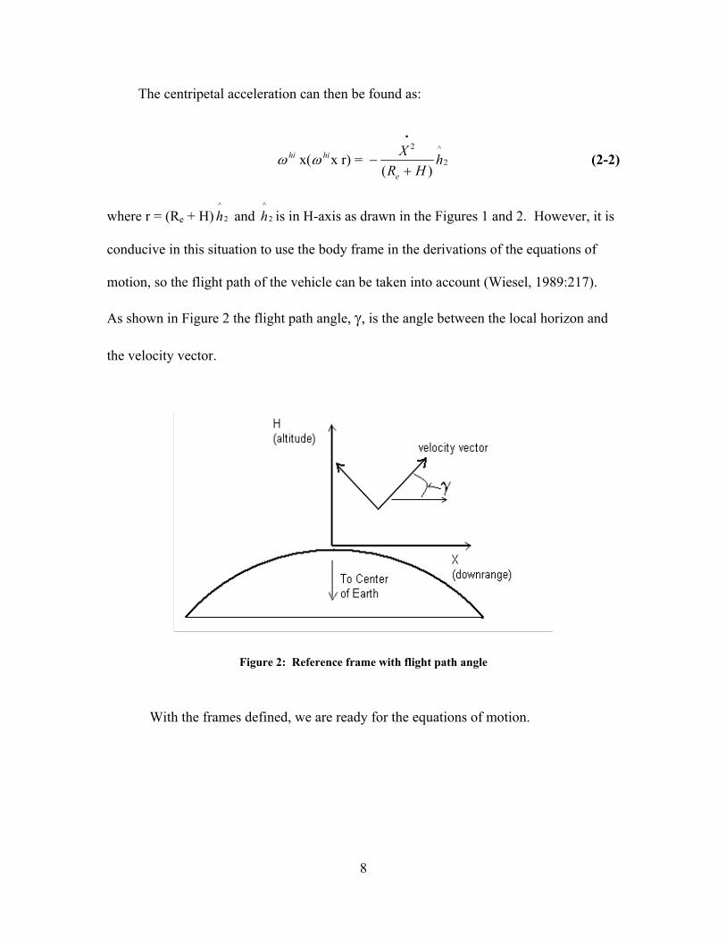
The centripetal acceleration can then be found as:
2 ^
2x x r) = ( )
.hi hi
e
X hR H
ω ω( −+
(2-2)
where r = (Re + H) and is in H-axis as drawn in the Figures 1 and 2. However, it is
conducive in this situation to use the body frame in the derivations of the equations of
motion, so the flight path of the vehicle can be taken into account (Wiesel, 1989:217).
As shown in Figure 2 the flight path angle, γ, is the angle between the local horizon and
the velocity vector.
^
2h^
2h
Figure 2: Reference frame with flight path angle
With the frames defined, we are ready for the equations of motion.
8

2.3 State Variables and Equations of Motion
The development of the equations of motion here is a modified form of those
presented in (Wiesel, 1989: 216-219). First, the state space vector must be defined. The
five elements used for this research are:
m – mass of the vehicle
H – altitude of the vehicle
X – distance downrange of the vehicle
V – velocity of the vehicle
γ − flight path angle of the vehicle
With the state vector defined, the equations of motion can be developed further.
Using Figure 3 as a reference, we can make some observations. First, the vehicle stays
on the H axis, therefore the vertical acceleration is and the downrange acceleration is
represented as
H&&
X&& . By geometry, the following equations can be produced:
cosdX Vdt
γ= (2-3)
sindH Vdt
γ= (2-4)
9

Figure 3: Diagram of Forces Acting on the Vehicle
As mentioned in the previous section, it is more conducive to use the body frame
instead of resolving into the vertical and horizontal frames. By doing so, the
accelerations of the vehicle can be summed up into acceleration along and transverse to
the vehicle’s axis. Considering that V is the velocity of the vehicle, and γ is the flight
path angle measured counterclockwise from the horizon, then dVdt
is the acceleration
produced along the axis of the vehicle, and dVdtγ is the acceleration transverse to the
vehicle’s axis.
Now, using Newton’s Second Law:
F ma=∑ (2-5)
10

We can then proceed to sum the forces of the vehicle. Again referencing Figure 3, we
find the forces acting on the vehicle are Thrust (T), Drag (D), gravity (mg), and
centripetal acceleration (2-2). Rotating the gravity and centripetal accelerations by the
flight path angle of the vehicle and summing the forces along the axis of the vehicle then
gives:
2
sin sin( )
.
e
m XF ma T D mgR H
γ γ= = − − ++∑ (2-6)
simplifying to:
2
( )( )
.
e
dV m Xm T D mgdt R H
sinγ= − − −+ (2-7)
Then similarly, summing the forces transverse to the axis of the vehicle produces:
2
cos cos( )
.
e
m XF ma mgR H
γ γ= = − ++∑ (2-8)
which then simplifies to:
2
( )( )
.
e
d m XmV mgdt R Hγ cosγ= − −
+ (2-9)
11

To find the mass flow rate of the vehicle the following equation was required:
. Tm
g Io sp= − (2-10)
where T is thrust, Isp is the specific impulse of the engine, and go is gravitational
acceleration at sea level. For the third stage, equation (2-10) holds true, however it does
not do so for the first and second stages. As the exact specifications are available for this
solid rocket motor, a double check reveals that with a burn time of 82 seconds, the mass
flow provided by (2-10) results in a total fuel burn that is greater than the actual available
fuel. Therefore, in the first two stages, the mass flow is determined by:
.
total mass of fuel
mburn time
= (2-11)
While it is most likely true that there is still some fuel left before the stage is jettisoned
and the fuel is probably not burned at a constant rate, this provides a reasonable model.
12

Therefore, to form the scalar equations of motion for the system, we gather the equations:
cosdX Vdt
γ=
sindH Vdt
γ=
2
(( )
.
e
dV m Xm T D mgdt R H
)sinγ= − − −+ (2-12)
2
( )( )
.
e
d m XmV mgdt R Hγ cosγ= − −
+
. Tm
g Io sp= −
In general, the equations of motion for non-linear time-dependent systems is
written:
(2-13) .
( , , )X f x u t=
Given x represents the state variables, u is representative of the control variables and t
represents time (Sears, 1997:14-15). This form is used by MATLAB, which is discussed
in the following chapter.
13
2.3 Hohmann Transfer
As will be discussed in Chapter 4, several options are available for achieving orbit.
One possible augmentation to the launch is the addition of a transfer orbit to insert the
vehicle into the proper orbit. The Hohmann Transfer is the most efficient use of available
fuel with the disadvantage of being the longest transfer available in terms of time.
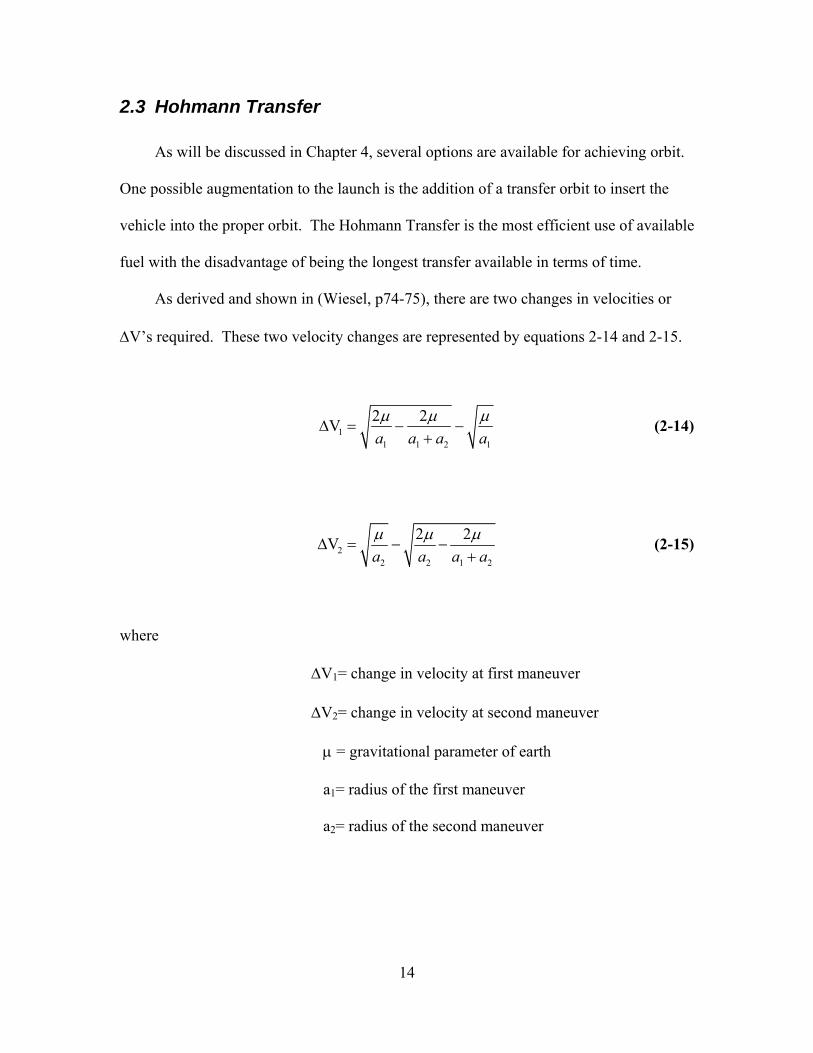
As derived and shown in (Wiesel, p74-75), there are two changes in velocities or
∆V’s required. These two velocity changes are represented by equations 2-14 and 2-15.
11 1 2
2 2Va a a a1
µ µ µ∆ = − −
+ (2-14)
22 2 1
2 2Va a a a2
µ µ µ∆ = − −
+ (2-15)
where
∆V1= change in velocity at first maneuver
∆V2= change in velocity at second maneuver
µ = gravitational parameter of earth
a1= radius of the first maneuver
a2= radius of the second maneuver
14

The gravitational parameter of earth (µ) is defined as 3.98601 x 10⁵ km3/s2 (Wiesel,
1989:323). A physical relationship between the variables in equations 2-14 and 2-15 can
best be seen in Figure 4 below:
Figure 4: Hohmann Transfer between two orbits (Wiesel, 1989:74)
15

Also of interest is the time of flight of the transfer orbit. A Hohmann transfer is basically
half of an elliptical orbit. So as seen in (Wiesel, 1989:75) the time between maneuvers is
given as:
3at π
µ∆ = (2-16)
where
1 2
2a aa +
= (2-17)
µ = 3.98601 x 10⁵ km3/s2
The time between maneuvers is especially of interest for mission planning.
16

III. ALGORITHMS
3.1 Introduction
In previous chapters the vehicle and equations of motion were discussed and
developed. In this chapter we discuss the algorithms used in the computer programs to
model the launch trajectories of the vehicle. Examples of the m-files can be found in
Appendix B. Before the algorithms can be truly discussed, the assumptions for this
problem need to be stated.
1. Drag is being neglected, i.e. D=0.
2. Vehicle specifications are as stated previously.
3. Third stage assumptions are accurate.
4. The vehicle has pitched to the full vertical position without expenditure of fuel
at launch.
5. The vehicle begins with a 300 mile per hour velocity at 20,000 feet.
6. The derivations and assumptions stated in the preceding chapters are assumed
correct.
The programs were written in the following units:
Mass = kilograms (kg)
Time = seconds (s)
Distance = meters (m)
Velocity = meters/second (m/s)
17
With the above assumptions, computer programs were written to solve the
boundary value problem for the gravity-turn equations of motion. These programs were
written in MATLAB 6.5 Student Edition and are commonly referred to as m-files in this
research. The entire trajectory profile boundary value problem was broken into three
parts. Each section represents a stage, as there is a discontinuity at the separation points.
Each program consists of two m-files. The first file, INITIALCOND provides initial
conditions and the initial state vector. The MATLAB command ODE45 then calls upon
the second m-file, LAUNCHEOMS in this case, that contains the equations of motion.
The routine continues for a set time period providing an output file of the state vector at
each time step. The following stage’s m-file then reads the last previous state vector and
runs an almost identical algorithm, the major changes being the initial conditions and in
the case of the third stage, the thrust. The end result is an output file with final
conditions in mass, altitude, downrange distance, velocity, and flight path angle of the
vehicle. The output file also contains the state vector at each of the iterations, providing
data for manipulation to be presented in the following chapter. Other programs were
used, but will be discussed later in the chapter. The purpose of these algorithms
ultimately is to find the altitude, velocity, and initial flight path angle that will provide a
zero flight path angle at burn out.
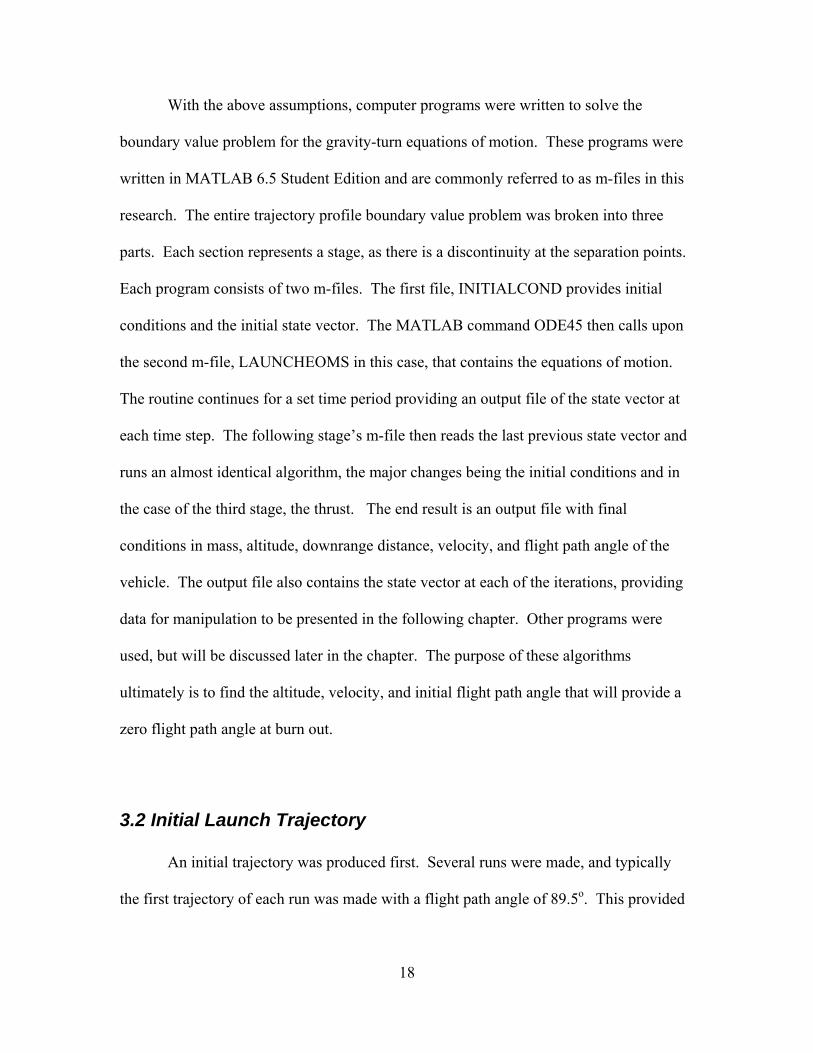
3.2 Initial Launch Trajectory An initial trajectory was produced first. Several runs were made, and typically
the first trajectory of each run was made with a flight path angle of 89.5o. This provided
18

a reference trajectory for each run. Obviously an initial flight path angle of 90o would
not be useful as there would not be a gravity-turn trajectory. The idea of gravity-turn is
that the vehicle would be in a vertical orientation, and then nudged over a small amount
so that the center of mass of the vehicle is no longer along the vertical axis, providing a
force from gravity that will be used to turn the vehicle.
The first program, INITIALCOND, is an m-file with a section noted for the initial
conditions. This file would provide the following:
• Initial 5 values of the state vector
• Time step and final time
• Prepare the output file to receive information
• Call on the second m-file through the ODE45 command
The second m-file for INITIALCOND would be LAUNCHEOMS. In
LAUNCHEOMS, the equations of motion are written in terms of the initial state vector.
The two files then work through the time period, which in this case is designated by the
burn time of the rocket motor of 82 seconds, to produce a final state vector for the stage.
The information is output to a text file at each time step so that the data can later be
examined and plotted.
At the end of INITIALCOND’s run, the vehicle has expended its first stage and
jettisons the dead weight. This produces a discontinuity in the change of mass that
dictates the need to write separate programs for each of the stages. The second program
is SECONDSTAGE and is paired with SECONDEOMS. The program SECONDSTAGE
is virtually identical to INITIALCOND except that it calls on a new initial mass, and then
calls on the last line of INITIALCOND’s output for the remainder of the initial state
19

vector. Then SECONDSTAGE calls SECONDEOMS, which again runs through the
equations of motion provided before. SECONDEOMS is identical to LAUNCHEOMS
except in the variables assigned to the state vector. The variables were named differently
to provide easier access for data manipulation. At the end of SECONDSTAGE, again
there is a discontinuity in mass from jettison of the second stage dead weight. Also note
that the third stage has a different thrust, mass flow rate, and burn time. Therefore
THIRDSTAGE is very similar to its predecessors but has very different values. It also
calls on the last vector provided by SECONDSTAGE. The output from THIRDSTAGE
is then provided in the output file, where a five-column matrix is given. Each stage has
it’s own text file for easier differentiation of the data. Of primary interest in the results
for this research is the final flight path angle. Two graphs would be plotted using the m-
file, PLOTFILE. The first graph would plot altitude vs. downrange distance, which in
essence is a modeling of the actual flight path of the vehicle as shown in Figure 4. The
second graph (Figure 5) plots altitude vs. flight path angle, which provides a graphical
means to observe the behavior of the vehicle’s attitude. With an initial reference
trajectory provided, we’re ready to extrapolate to the desired point of a zero degree flight
path angle at burn out.
20

Figure 5: Altitude vs Downrange Distance for Initial γo of 89.5o
21

Figure 6: Altitude vs Gamma γ for γo of 89.5o
22

3.3 Extrapolation to Zero Flight Path Angle at Burn Out
The goal here is to find the correct initial conditions that provide for a zero degree
flight path angle at burnout. To do this, a second trajectory is found using the same
procedure as for the initial trajectory above. However, this trajectory begins with an
angle of 88.5o as it’s initial flight path angle γο. After running the m-files through with
this initial condition, a second trajectory is formed as shown in Figures 7 and 8 below.
Figure 7: Altitude vs Distance for γo of 88.5o
23

Figure 8: Altitude vs Flight Path Angle γο for γo of 88.5o
As shown in these charts, the final γ is not equal to zero. Here another m-file
routine called NEWGAMMA is applied. This program requires values to be input into
the file directly. The initial flight path angles, γo, and the final angles, γf, from both runs
are input here. The program then runs a simple formula to find the next γo:
new old old
oo o
ff
γγ γ γγ
∆= −
∆ (3-1)
24
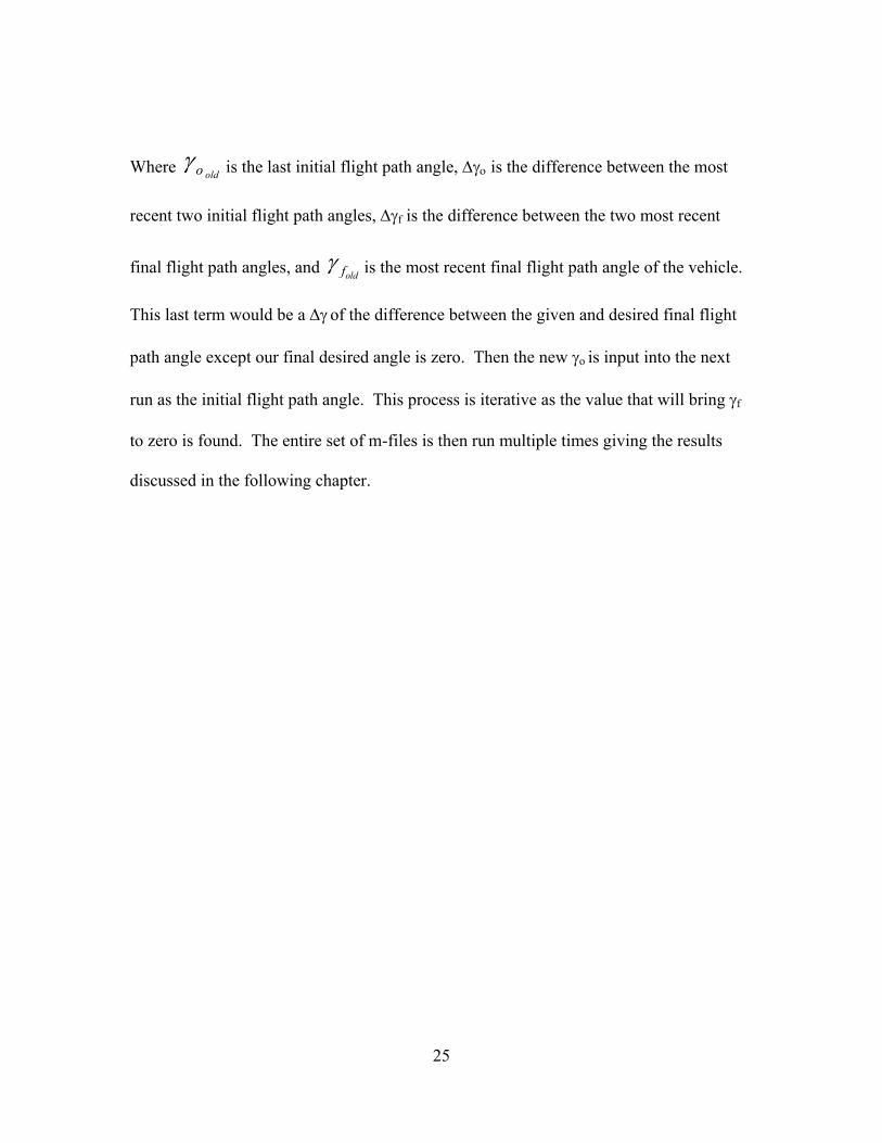
Where oldoγ is the last initial flight path angle, ∆γο is the difference between the most
recent two initial flight path angles, ∆γf is the difference between the two most recent
final flight path angles, and oldfγ is the most recent final flight path angle of the vehicle.
This last term would be a ∆γ of the difference between the given and desired final flight
path angle except our final desired angle is zero. Then the new γo is input into the next
run as the initial flight path angle. This process is iterative as the value that will bring γf
to zero is found. The entire set of m-files is then run multiple times giving the results
discussed in the following chapter.
25

IV. RESULTS AND DISCUSSION
4.1 Introduction
This chapter presents the results found in the gravity-turn trajectory modeling of
the Boeing AirLaunch based vehicle. The only payload considered in this research was
the Space Maneuver Vehicle (SMV) that is currently in development for the Air Force.
This is considered to be approximately 3,000 kg (7,500 lb) of payload mass. With the
vehicle described in previous chapters as the launch vehicle, the gravity-turn m-files can
now be run.
4.2 Initial Results
Since the engines are solid rocket motors, they are not capable of throttling by
design. This provides that there is no capability for changing thrust during the burn
sequences. Intuition should prove that given these facts this method has a fixed altitude
at which the final flight path angle γf goes to zero. Using the procedures described in the
previous chapter, the first runs were found to go to zero at the state described in Table 3.
This run is referred to as case 1 for the remainder of this thesis.
26

Table 3: Final conditions of case 1 Initial Flight Path Angle γo 87.51904o
Altitude 81433.5009 meters
Downrange Distance 504090.589 meters
Velocity 7344.29656 m/s
As can be seen in Table 3, the final altitude is only 81.4 kilometers. It is
immediately obvious that this is not high enough to be in low earth orbit. For this
research, an orbit of 250 kilometers was chosen as the target altitude. Several ideas were
approached to alter the final altitude. Since the vehicle is powered by solid rocket
motors, there is no capability for variation of thrust or burn time. One possibility,
therefore, is to look into coasting the vehicle between stages in order to gain a higher
altitude.
4.3 Vehicle Coasting
In order to reach higher orbit altitudes, coasting the vehicle was investigated. This
involves waiting between stages before igniting the next stage. After the previous stage
has burned out, it will be jettisoned and the vehicle will then continue on for a specified
amount of time under no thrust. This is referred to as coasting as the vehicle is under no
power. By coasting, the vehicle will continue to gain altitude while conserving fuel and
can therefore get to higher altitudes. To insert coasting, m-files were created that ran the
equations of motion without thrust or mass flow. Similar to the routines described above,
27

the initial flight path angle had to be varied until a final flight path angle of zero was
attained. Several runs were attempted while varying the coast times between stage
ignitions. As discussed before, drag is assumed to be negligible, which could cause
differences in real world scenarios. The results varied as presented in the remainder of
this section.
The first cases attempted were made while keeping the coast times consistent with
each other. In case 2, only a five second coast was considered. As seen in Figure 9 and
Table 4 this showed that only a small change was attained. Obviously a much larger
coast time is needed.
Table 4: Final conditions of case 2 Initial Flight Path Angle γo 87.88o
Altitude 86441.6828 meters
Downrange Distance 505497.292 meters
Velocity 7263.80507 m/s
28

Figure 9: Launch trajectory for case 2
From case 2, a jump to a coast of thirty-five seconds between stages was
performed in case 3 to see how large a difference could be found. As seen in Figure 10
and Table 5, a much higher altitude is reached than the previous runs. However, an
altitude of 121 km is still fairly low for an orbit.
29

Figure 10: Launch trajectory for case 3
Table 5: Final conditions for case 3 Initial Flight Path Angle γo 89.57o
Altitude 121398.648 meters
Downrange Distance 464387.699 meters
Velocity 6644.82810 m/s
30

In case 4, a coast time of sixty seconds between stages was investigated. This
however had some serious problems as seen in Figure 11 and Table 6. It was found that
the flight path did not converge to zero for this coast time, and the vehicle would impact
the surface during the second stage burn. This is obviously a bad thing to happen to the
launch vehicle.
Figure 11: Launch trajectory for case 4
31

Table 6: Final conditions after case 4
Initial Flight Path Angle γo 89.9o
Altitude -70583.0107 meters
Downrange Distance 26483.1574 meters
Velocity 3.24739556 m/s
After several experimental runs, it was determined that a coast time larger than
approximately 50 seconds during the first coast caused the vehicle’s flight path angle to
degrade too quickly. The decision was then made to confine the first coast time to 50
seconds or less. Then the second coast times were varied to attain higher altitudes. In
case 5, the first coast stage was set to 40 seconds and then run with second coast times of
60 seconds, 90 seconds and 120 seconds which are represented in Figures 12, 13, and 14,
respectively. These figures give a representation of possible altitudes to reach, as all
altitudes between them are capable of being achieved through modification of the coast
times. Also note the large difference in altitudes between the different coast times. This
gives evidence that the vehicle has feasibility to reach more reasonable orbital altitudes.
32

Figure 12: Launch trajectory of case 5 with second stage coast of 60 seconds
33

Figure 13: Launch trajectory of case 5 with a second stage coast of 90 seconds
34

Figure 14: Launch trajectory of case 5 with a second stage coast of 120 seconds
The highest altitude achieved through the case 5 trajectories was approximately
237 km. This is much closer to the more desirable orbits. Attempts to reach higher orbits
with case 5’s first coast were unproductive. So to achieve slightly higher altitudes in case
6, the first coast time was extended to 50 seconds and the second coast stage time was set
35

at 120 seconds. This second stage coast time gave the highest altitude previously, and is
therefore a logical starting place. The results of case 6 are shown in Figure 15 and Table
7 below.
Figure 15: Launch trajectory of case 6
Table 7: Final conditions of case 6
Initial Flight Path Angle γo 89.98o
Altitude 228092.170 meters
Velocity 5450.60642 m/s
36

As seen in Figure 14 and Table 7, the altitude reached is actually less than that of
the highest achievable in case 5. After several iterations, a second coast stage of 160
seconds chosen for case 7. The trajectory and final conditions of case 7 are given in
Figure 16 and Table 8, respectively.
Figure 16: Launch trajectory with case 7
37

Table 8: Final conditions after case 7 Initial Flight Path Angle γo 89.9975o
Altitude 262427.963 meters
Velocity 4584.99328 m/s
As seen in Table 8, the vehicle is finally above 250 km in altitude. Now that
decent altitudes are capable of being reached, the vehicle was then set up to achieve a
certain altitude.
For case 8, a goal was set for a 250 km orbit. A trajectory was then found that
would approach 250 km as the flight path angle came to zero and then the vehicle was
allowed to keep a zero flight path angle and accelerate in the orbit. The results of case 8
produce the trajectory and final conditions shown in Figure 17 and Table 9 below.
38
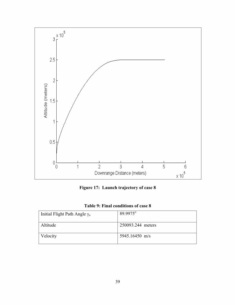
Figure 17: Launch trajectory of case 8
Table 9: Final conditions of case 8
Initial Flight Path Angle γo 89.9975o
Altitude 250093.244 meters
Velocity 5945.16450 m/s
39

Of interest to the research at this point is the velocity needed to maintain a
circular orbit. This velocity is governed by the equation:
cvrµ
= (4-1)
where µ is the gravitational parameter of the local earth system, and is given as
3.98601x10⁵ km3/s2, and r = (Re + H), with Re given as 6378.135 km. Assuming an
altitude (H) of 250 km, it is found that the velocity required to maintain this circular orbit
is approximately 7.754 km/s. Given the final velocity shown in Table 9 of 5.945 km/s, it
is obvious that the vehicle will not remain in this orbit. So an addition of velocity is
required to maintain the desired orbit. As previously stated, the payload of the Boeing
AirLaunch System for this research is assumed to be the Space Maneuvering Vehicle
(SMV). The SMV is still in development, however by design it will be capable of 3200
m/s of additional velocity commonly referred to as ∆V (“Space Maneuver Vehicle Fact
Sheet”: 2004). For the purpose of reaching the desired orbital velocity, it is assumed that
the SMV will be used to produce the required ∆V of 1809 m/s, which is well within its
capabilities. Assuming the SMV accelerates at the same rate that the third stage did,
about 100 m/s2, this will add approximately 18 seconds to the launch time. This gives the
time from ignition to on orbit as approximately 429 seconds or 7.15 minutes.
40

4.4 Hohmann Transfer Results
Another possibility for orbital insertion is a transfer orbit into the desired plane.
Since this vehicle has a limited amount of fuel available to it, a Hohmann transfer is the
best choice to make the transfer when time to orbit is not an issue. As discussed in
Chapter 2, the Hohmann transfer consists of two changes in velocity to first put the
vehicle onto an elliptical orbit and then another to place the orbiter into the desired orbit.
For the first consideration, case 1 was taken as the launch trajectory and a 250 km
orbit again was chosen as the target. This investigation is here dubbed case 9. First, the
vehicle at the end of case 1 is at approximately 81.43 km and traveling at 7.344 km/s. In
order to take advantage of equations 2-14 and 2-15, the vehicle must first be accelerated
to the correct velocity to maintain the given orbit. This can be found using equation 4-1
and determining the difference in velocities. Equations 2-14 and 2-15 can then be used to
determine the ∆V’s required for the transfer, and equation 2-16 is used to find the time of
flight of the vehicle. The results are shown below in Table 10.
Table 10: Case 9 results for Hohmann transfer
∆V required for inner orbit 0.511 km/s
∆V1 for the Hohmann transfer 0.0504 km/s
∆V2 for the Hohmann transfer 0.0501 km/s
Total ∆V required 0.6115 km/s
Time of flight, ∆t 2634.09 s or 43.9 minutes
41

With a total ∆V required of 0.6115 km/s, this maneuver is well within the range
of the SMV’s capability of a 3.2 km/s ∆V. This shows an excellent possibility for
launching to orbit.
In case 10, the vehicle is assumed to be at the end of case 6. At an altitude of
approximately 228.092 km and velocity of 5.45 km/s, the ∆V’s required to achieve a 250
km orbit are shown in Table 11.
Table 11: Case 10 results for Hohmann transfer
∆V required for inner orbit 2.3177 km/s
∆V1 for the Hohmann transfer 0.00643 km/s
∆V2 for the Hohmann transfer 0.00642 km/s
Total ∆V required 2.3305 km/s
Time of flight, ∆t 2678.49 s or 44.6 min
The results of case 10 are still within the range of the available ∆V of the SMV,
however, case 9 is a much more efficient profile. Interestingly this poses an unexpected
scenario. The initial launch trajectory posed in case 1 barely reaches the altitude of 80
km but is far more efficient using a Hohmann transfer than coasting is, as displayed in
case 8. Also of interest here is that the higher trajectories reached by coasting have a
higher total ∆V than the trajectory that has no coasting. This is primarily due to the fact
that as the vehicle coasts it is slowing down due to gravity losses while the launch
trajectory without coasting provides a velocity very near the orbital velocity needed.
42
The results shown in this chapter demonstrate that the vehicle represented in this
research is capable of reaching a prescribed altitude through a gravity-turn trajectory with
supplementation. Surprising to this researcher, the initial launch augmented with a
Hohmann transfer is the most fuel efficient of the cases investigated. Using the
capability of an air launch platform, this vehicle is capable of intercepting the proper
orbit of a target and launching at such a time that at engines cut off, the target is
alongside. For a fuel-efficient attempt, the vehicle could rendezvous at the end of the
Hohmann transfer, and for a faster intercept the vehicle can use coasting to achieve the
proper orbital altitude and use the SMV to accelerate into the orbital plane, as was shown
in case 8. The following chapter discusses this as well as recommendations for future
investigation.
43
V. CONCLUSIONS AND RECOMMENDATIONS
5.1 Conclusions
The goal of this research was to evaluate the feasibility of a coplanar, gravity-turn
launch trajectory using a vehicle based heavily upon the Boeing AirLaunch System. The
results from the previous chapter demonstrate that the vehicle described in this research is
capable of reaching reasonable altitudes in low earth orbit with modifications to its
trajectory through coasting and transfer orbits. Since the payload of the vehicle can be
considered in essence a fourth stage, there are a considerable number of options that can
be used to achieve a desired orbit. This research limited these options to coasting and
Hohmann transfers.
Since the vehicle can be positioned literally anywhere in the world, the launch
scenarios investigated are quite possible. With actual information on the third stage and
the Space Maneuver Vehicle (SMV), calculations of a direct to rendezvous launch is
possible. This would simply require determining the correct launch time as dictated by
the target vehicle. The mission could be completed in however long it would take the
Boeing 747 launch vehicle to arrive at the proper location.
This research provides an interesting and insightful look at gravity-turn launch
trajectories and the use of solid rocket motors in a responsive launch situation. It shows
that with coasting and transfer orbits, most low earth orbits are attainable, and direct to
rendezvous is feasible. As an interesting development, it also demonstrated that the most
efficient launch was to a lower altitude followed by a Hohmann transfer to the desired
44

altitude. The tradeoff here of course is time to rendezvous at the correct orbit. Case 8
achieves engines off on orbit at just over 7 minutes, where as case 9 reaches the target
orbit at approximately 48 minutes after engine ignition.
5.2 Recommendations
The most obvious next step for this system is to find actual specifications for the
third stage and SMV. This may greatly affect the system if actual specifications are
much greater or less than the assumed values. Also of interest is to add drag into the
equation. The introduction of drag will primarily affect the first stage and possibly the
first coasting stage. Another point of interest would be to reproduce the equations of
motion in the three dimensional earth centered reference frame. With the three-
dimensional models, a launch to rendezvous can be examined in depth for the purposes of
mission planning.
As the field of space launch continues to evolve, the desirable capabilities of
launch on demand and direct to rendezvous launch will become more and more feasible
in reality. Platforms like the Boeing AirLaunch System are not too far into the future.
Orbital already operates a much smaller payload class on a similar platform called
Pegasus. The results of this thesis offer an insight into the possible next evolution of this
developing technology. The ability of launching directly to rendezvous has significant
advantages in civilian and military aspects as well as peacetime and wartime missions.
45

The portability of an air launch system allows the concept of reaching virtually any
orbital plane desirable. The research presented here poses some interesting possibilities
for this type of technology in the future.
46

APPENDIX A: Code Summary
FIRSTCOASTEOM
TYPE: Subroutine m-file
PURPOSE: This routine provides the equations of motion to iterate through the first
coasting stage conditions. This file provides the changes in the state
variables per time.
INPUTS: State vector
OUTPUTS: State vector
CALLS: None
AUTHOR: David W. Callaway
FIRSTSTAGECOAST
TYPE: Main Program m-file
PURPOSE: This program solves a boundary value problem for the gravity-turn
trajectory of the first coasting stage.
INPUTS: Final state vector from first stage burn and new initial mass
OUTPUTS: Final state vector after coasting
CALLS: FIRSTCOASTEOM
INITIALCOND
AUTHOR: David W. Callaway
47

INITIALCOND
TYPE: Main Program m-file
PURPOSE: This program solves a boundary value problem for the gravity-turn trajectory of the first stage burning.
INPUTS: Initial state vector
OUTPUTS: Final state vector for first stage
CALLS: LAUNCHEOMS
AUTHOR: David W. Callaway
LAUNCHEOMS
TYPE: Subroutine m-file
PURPOSE: This routine provides the equations of motion to iterate through the first stage burn conditions. This file provides the changes in the state variables per time.
INPUTS: State vector
OUTPUTS: State vector
CALLS: None
AUTHOR: David W. Callaway
48

NEWGAMMA
TYPE: Main Program m-file
PURPOSE: This program determines the change in final flight path angle per change in initial flight path angle. It then finds the new initial flight path angle for the next iteration.
INPUTS: Initial flight path angles from the two previous iterations Final flight path angles from the two previous iterations
OUTPUTS: Initial flight path angle
CALLS: None
AUTHOR: David W. Callaway
PLOTFILE
TYPE: Main Program m-file
PURPOSE: This program calls the iterated state vectors from all stages of the launch and plots them for data analysis.
INPUTS: All Iterations of state vectors
OUTPUTS: Downrange distance vs. Altitude plot Flight path angle vs. Altitude plot
CALLS: output from: INITIALCOND
FIRSTSTAGECOAST SECONDSTAGE SECONDSTAGECOAST THIRDSTAGE AUTHOR: David W. Callaway
49

SECONDCOASTEOMS
TYPE: Subroutine m-file
PURPOSE: This routine provides the equations of motion to iterate through the second coasting stage conditions. This file provides the changes in the state variables per time.
INPUTS: State vector
OUTPUTS: State vector
CALLS: None
AUTHOR: David W. Callaway
SECONDEOMS
TYPE: Subroutine m-file
PURPOSE: This routine provides the equations of motion to iterate through the second stage burn conditions. This file provides the changes in the state variables per time.
INPUTS: State vector
OUTPUTS: State vector
CALLS: None
AUTHOR: David W. Callaway
50

SECONDSTAGE
TYPE: Main Program m-file
PURPOSE: This program solves a boundary value problem for the gravity-turn trajectory of the second stage burning.
INPUTS: Final state vector of either first stage or first coasting stage, dependent
on case. OUTPUTS: Final state vector for second stage
CALLS: SECONDEOMS
AUTHOR: David W. Callaway
SECONDSTAGECOAST
TYPE: Main Program m-file
PURPOSE: This program solves a boundary value problem for the gravity-turn trajectory of the second coasting stage.
INPUTS: Final state vector of second stage
OUTPUTS: Final state vector for second coasting stage
CALLS: SECONDCOASTEOMS
AUTHOR: David W. Callaway
51
THIRDEOMS
TYPE: Subroutine m-file
PURPOSE: This routine provides the equations of motion to iterate through the third stage burn conditions. This file provides the changes in the state variables per time.
INPUTS: State vector
OUTPUTS: State vector
CALLS: None
AUTHOR: David W. Callaway
THIRDSTAGE
TYPE: Main Program m-file
PURPOSE: This program solves a boundary value problem for the gravity-turn trajectory of the third stage burning.
INPUTS: Final state vector of second stage or second coasting stage, dependent on
case OUTPUTS: Final state vector for third stage
CALLS: THIRDEOMS
AUTHOR: David W. Callaway
52

APPENDIX B: M-Files
The m-files presented here are from case 7. It should be noted that they are
provided here in alphabetical order; however, they must be run from the same file in the
order INITIALCOND, FIRSTSTAGECOAST, SECONDSTAGE,
SECONDSTAGECOAST, THIRDSTAGE, and PLOTFILE.
FIRSTCOASTEOM
% eoms for firststage coast %LT Callaway, Thesis %Trajectory model function [ycdot]=firstcoasteom(t,yc) global mdot T Re ge tstep %EOM's for 2-D launch %y0=[mnot Hnot Xnot Vnot gammanot}; %change in mass mdot ycdot(1,1)=0; %change in altitude Hdot ycdot(2,1)=yc(4)*sin(yc(5)); %change in horizontal distance Xdot ycdot(3,1)=yc(4)*cos(yc(5)); %change in Velocity ycdot(4,1)=(1/yc(1))*(T-(yc(1)*ge-yc(1)*((yc(4)*cos(yc(5)))^2)/(Re+yc(2)))*sin(yc(5))); %change in gamma ycdot(5,1)=-(1/yc(1))*(1/yc(4))*(yc(1)*ge-yc(1)*((yc(4)*cos(yc(5)))^2)/(Re+yc(2)))*cos(yc(5));
53

FIRSTSTAGECOAST % coast stage 1 %LT Callaway, Thesis %Trajectory model %Intial Conditions: close all file=fopen('C:\thesis\withcoast\firststagecoast.txt','w+'); fprintf(file,'mass \t \t \t altitude \t \t \t X \t \t \t V \t \t \t gamma \n'); global mdot T Re ge tstep %Times tstep=1; %sec tfinal=50; %sec % Constants -------------------------- T=0; %Thrust in N mdot=0; %mass flow is considered constant (kg/s); Re=6378135; %Radius of earth in meters; ge=9.81; %gravity g; %%%%%%%%%%%%%%%%%%%%%%%%%%%%%%%%%%%%%%%%%%% % Initial Conditions mnot=83388.874893; %total mass - first stage %%%%%%%%%%%%%%%%%%%%%%%%%%%%%%%%%%%%%%%%%%% % yyy0=[mnot Hnot Xnot Vnot gammanot]; yc0=[mnot y(83,2) y(83,3) y(83,4) y(83,5)]; % Integrate the equations of motion options = odeset('RelTol',1e-7,'AbsTol',1e-10*ones(1,5)); [t,yc] = ODE45('firstcoasteom',0:tstep:tfinal,yc0,options); out=[yc(:,2) yc(:,3) yc(:,4) yc(:,5)]; fprintf(file,'%2.8e \t %2.8e \t %2.8e \t %2.8e \n',out'); % fprintf(file,'%2.8e \t %2.8e \t %2.8e \t %2.8e \t %2.8e \n',yc'); fclose(file);
54

INITIALCOND %LT Callaway, Thesis %Trajectory model %Intial Conditions: clear close all file=fopen('C:\thesis\withcoast\firststage.txt','w+'); fprintf(file,'mass \t \t \t altitude \t \t \t X \t \t \t V \t \t \t gamma \n'); global mdot T Re ge tstep %Times tstep=1; %sec tfinal=82; %sec % Constants -------------------------- T=1650245.73705; %Thrust in N mdot=592.64056; %mass flow is considered constant (kg/s); Re=6378135; %Radius of earth in meters; ge=9.81; %gravity g; %%%%%%%%%%%%%%%%%%%%%%%%%%%%%%%%%%%%%%%%%%% % Initial Conditions mnot=136077.711; %total mass in kg gammanot=89.9975*pi/180; %gamma must be in radians; Vnot=134.112; %Initial velocity 300 mph, but in meters/sec: Hnot=6096; %Initial Altitude... 20kft...in meters Xnot=0; %Initial X position %%%%%%%%%%%%%%%%%%%%%%%%%%%%%%%%%%%%%%%%%%% y0=[mnot Hnot Xnot Vnot gammanot]; % Integrate the equations of motion options = odeset('RelTol',1e-7,'AbsTol',1e-10*ones(1,5)); [t,y] = ODE45('launcheoms',0:tstep:tfinal,y0,options); out=[y(:,2) y(:,3) y(:,4) y(:,5)]; fprintf(file,'%2.8e \t %2.8e \t %2.8e \t %2.8e \n',out'); %fprintf(file,'%2.8e \t %2.8e \t %2.8e \t %2.8e \t %2.8e \n',y'); fclose(file);
55

LAUNCHEOMS % Launcheoms for first stage % LT Callaway, Thesis %Trajectory model function [ydot]=launcheoms(t,y) global mdot T Re ge tstep %EOM's for 2-D launch %y0=[mnot Hnot Xnot Vnot gammanot}; %change in mass mdot ydot(1,1)=-592.64056; %change in altitude Hdot ydot(2,1)=y(4)*sin(y(5)); %change in horizontal distance Xdot ydot(3,1)=y(4)*cos(y(5)); %change in Velocity ydot(4,1)=(1/y(1))*(T-(y(1)*ge-y(1)*((y(4)*cos(y(5)))^2)/(Re+y(2)))*sin(y(5))); %change in gamma ydot(5,1)=-(1/y(1))*(1/y(4))*(y(1)*ge-y(1)*((y(4)*cos(y(5)))^2)/(Re+y(2)))*cos(y(5)); NEWGAMMA %dgamma/dgammanot program %dgamma= old gamma - new gamma gammao=5.25671725e-001; gamman=1.15971452e-002; dgamma=gammao-gamman %radians % dgammanot= |new gamma - previous gamma| gammanotnew=89.78; gammanotold=89.9; dgammanot=gammanotold-gammanotnew %degrees deltagammanot=(dgammanot)*(gamman)/(dgamma) %degrees newgammanot=gammanotnew-deltagammanot
56

PLOTFILE hold on; %plotting altitude vs X plot(y(:,3),y(:,2)); plot(yc(:,3),yc(:,2)); plot(yy(:,3),yy(:,2)); plot(ycc(:,3),ycc(:,2)); plot(yyy(:,3),yyy(:,2)); %plotting altitude vs gamma % plot(y(:,5),y(:,2)); % plot(yc(:,5),yc(:,2)); % plot(yy(:,5),yy(:,2)); % plot(ycc(:,5),ycc(:,2)); % plot(yyy(:,5),yyy(:,2)); SECONDCOASTEOMS % eoms for second stage coast function [yccdot]=secondcoasteoms(t,ycc) global mdot T Re ge tstep %EOM's for 2-D launch %y0=[mnot Hnot Xnot Vnot gammanot}; %change in mass mdot yccdot(1,1)=0; %change in altitude Hdot yccdot(2,1)=ycc(4)*sin(ycc(5)); %change in horizontal distance Xdot yccdot(3,1)=ycc(4)*cos(ycc(5)); %change in Velocity yccdot(4,1)=(1/ycc(1))*(T-(ycc(1)*ge-ycc(1)*((ycc(4)*cos(ycc(5)))^2)/(Re+ycc(2)))*sin(ycc(5))); %change in gamma yccdot(5,1)=-(1/ycc(1))*(1/ycc(4))*(ycc(1)*ge-ycc(1)*((ycc(4)*cos(ycc(5)))^2)/(Re+ycc(2)))*cos(ycc(5));
57

SECONDEOMS % Launcheoms for second stage function [yydot]=secondeoms(t,yy) global mdot T Re ge tstep %EOM's for 2-D launch %y0=[mnot Hnot Xnot Vnot gammanot}; %change in mass mdot yydot(1,1)=-592.64056; %change in altitude Hdot yydot(2,1)=yy(4)*sin(yy(5)); %change in horizontal distance Xdot yydot(3,1)=yy(4)*cos(yy(5)); %change in Velocity yydot(4,1)=(1/yy(1))*(T-(yy(1)*ge-yy(1)*((yy(4)*cos(yy(5)))^2)/(Re+yy(2)))*sin(yy(5))); %change in gamma yydot(5,1)=-(1/yy(1))*(1/yy(4))*(yy(1)*ge-yy(1)*((yy(4)*cos(yy(5)))^2)/(Re+yy(2)))*cos(yy(5));
58

SECONDSTAGE % SECOND STAGE INIITIAL CONDITIONS %Intial Conditions: close all file=fopen('C:\thesis\withcoast\secondstage.txt','w+'); fprintf(file,'mass \t \t \t altitude \t \t \t X \t \t \t V \t \t \t gamma \n'); global mdot T Re ge tstep %Times tstep=1; %sec tfinal=82; %sec % Constants -------------------------- T=1650245.73705; %Thrust in N mdot=592.64056; %mass flow is considered constant (kg/s); Re=6378135; %Radius of earth in meters; ge=9.81; %gravity g; %%%%%%%%%%%%%%%%%%%%%%%%%%%%%%%%%%%%%%%%%%% % Initial Conditions mnot=83388.874893; %total mass - first stage mass in kg % gammanot=1.36707253; %gamma must be in radians; % Vnot=564.206512; %Velocity from end of 1st stage, but in meters/sec: % Hnot=30732.3097; %Altitude from previous run % Xnot=2685.21896; %Initial X position %%%%%%%%%%%%%%%%%%%%%%%%%%%%%%%%%%%%%%%%%%% % yy0=[mnot Hnot Xnot Vnot gammanot]; yy0=[mnot yc(51,2) yc(51,3) yc(51,4) yc(51,5)]; % Integrate the equations of motion options = odeset('RelTol',1e-7,'AbsTol',1e-10*ones(1,5)); [t,yy] = ODE45('secondeoms',0:tstep:tfinal,yy0,options); out=[yy(:,2) yy(:,3) yy(:,4) yy(:,5)]; fprintf(file,'%2.8e \t %2.8e \t %2.8e \t %2.8e \n',out'); %fprintf(file,'%2.8e \t %2.8e \t %2.8e \t %2.8e \t %2.8e \n',yy'); fclose(file);
59

SECONDSTAGECOAST % coast stage 2 %LT Callaway, Thesis %Trajectory model %Intial Conditions: close all file=fopen('C:\thesis\withcoast\secondstagecoast.txt','w+'); fprintf(file,'mass \t \t \t altitude \t \t \t X \t \t \t V \t \t \t gamma \n'); global mdot T Re ge tstep %Times tstep=1; %sec tfinal=160; %sec % Constants -------------------------- T=0; %Thrust in N mdot=0; %mass flow is considered constant (kg/s); Re=6378135; %Radius of earth in meters; ge=9.81; %gravity g; %%%%%%%%%%%%%%%%%%%%%%%%%%%%%%%%%%%%%%%%%%% % Initial Conditions mnot=30700.027786; %total mass - stages 1 and 2 %%%%%%%%%%%%%%%%%%%%%%%%%%%%%%%%%%%%%%%%%%% % yyy0=[mnot Hnot Xnot Vnot gammanot]; ycc0=[mnot yy(83,2) yy(83,3) yy(83,4) yy(83,5)]; % Integrate the equations of motion options = odeset('RelTol',1e-7,'AbsTol',1e-10*ones(1,5)); [t,ycc] = ODE45('secondcoasteoms',0:tstep:tfinal,ycc0,options); out=[ycc(:,2) ycc(:,3) ycc(:,4) ycc(:,5)]; fprintf(file,'%2.8e \t %2.8e \t %2.8e \t %2.8e \n',out'); % fprintf(file,'%2.8e \t %2.8e \t %2.8e \t %2.8e \t %2.8e \n',ycc'); fclose(file);
60
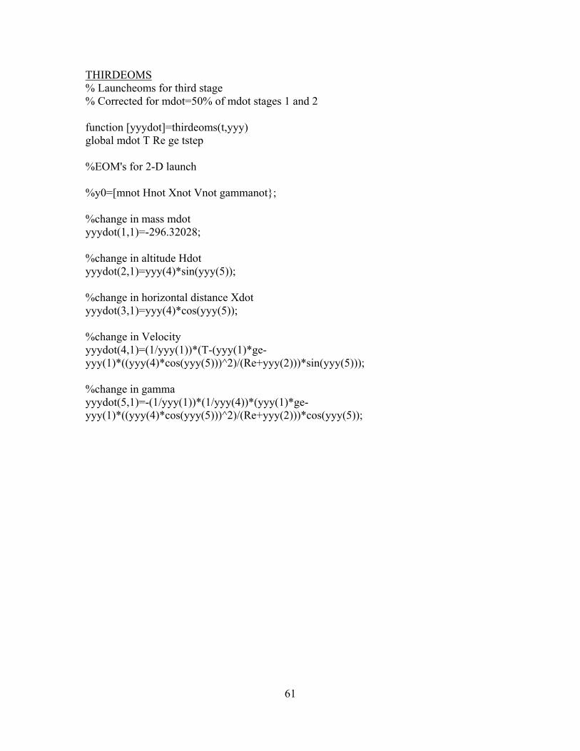
THIRDEOMS % Launcheoms for third stage % Corrected for mdot=50% of mdot stages 1 and 2 function [yyydot]=thirdeoms(t,yyy) global mdot T Re ge tstep %EOM's for 2-D launch %y0=[mnot Hnot Xnot Vnot gammanot}; %change in mass mdot yyydot(1,1)=-296.32028; %change in altitude Hdot yyydot(2,1)=yyy(4)*sin(yyy(5)); %change in horizontal distance Xdot yyydot(3,1)=yyy(4)*cos(yyy(5)); %change in Velocity yyydot(4,1)=(1/yyy(1))*(T-(yyy(1)*ge-yyy(1)*((yyy(4)*cos(yyy(5)))^2)/(Re+yyy(2)))*sin(yyy(5))); %change in gamma yyydot(5,1)=-(1/yyy(1))*(1/yyy(4))*(yyy(1)*ge-yyy(1)*((yyy(4)*cos(yyy(5)))^2)/(Re+yyy(2)))*cos(yyy(5));
61

THIRDSTAGE % Third STAGE INIITIAL CONDITIONS %Intial Conditions: close all file=fopen('C:\thesis\withcoast\thirdstage.txt','w+'); fprintf(file,'mass \t \t \t altitude \t \t \t X \t \t \t V \t \t \t gamma \n'); global mdot T Re ge tstep %Times tstep=1; %sec tfinal=84; %sec rounded down from 84.9 seconds % Constants -------------------------- T=813932.5451; %Thrust in N mdot=592.64056; %mass flow is considered constant (kg/s); Re=6378135; %Radius of earth in meters; ge=9.81; %gravity g; %%%%%%%%%%%%%%%%%%%%%%%%%%%%%%%%%%%%%%%%%%% % Initial Conditions mnot=30700.027786; %total mass - first stage mass in kg % gammanot=1.13822111; %gamma must be in radians; % Vnot=2241.82678; %Velocity from end of 2nd stage, in meters/sec: % Hnot=124507.332; %Altitude from previous run % Xnot=37516.3229; %Initial X position third stage %%%%%%%%%%%%%%%%%%%%%%%%%%%%%%%%%%%%%%%%%%% % yyy0=[mnot Hnot Xnot Vnot gammanot]; yyy0=[mnot ycc(161,2) ycc(161,3) ycc(161,4) ycc(161,5)]; % Integrate the equations of motion options = odeset('RelTol',1e-7,'AbsTol',1e-10*ones(1,5)); [t,yyy] = ODE45('thirdeoms',0:tstep:tfinal,yyy0,options); out=[yyy(:,2) yyy(:,3) yyy(:,4) yyy(:,5)]; fprintf(file,'%2.8e \t %2.8e \t %2.8e \t %2.8e \n',out'); % fprintf(file,'%2.8e \t %2.8e \t %2.8e \t %2.8e \t %2.8e \n',yyy'); fclose(file);
62

Bibliography
“Castor 120.” Online Thiokol product fact sheets. n. pag. http://www.thiokol.com/castor2.htm. 23 November 2003.
“Phantom Works AirLaunch System (ALS).” Boeing project home page. n. pag.
http://www.boeing.com/phantom/als.html. 23 November 2003. Platt, Michael H. Full Lyapunov Exponent Placement in Reentry Trajectories. MS
Thesis, AFIT/GA/ENY/95D-03. School of Engineering, Air Force Institute of Technology (AU), Wright-Patterson AFB, OH, December 1995 (AD-A303109).
Sears, Gregory B. Optimal Non-Coplanar Launch to Quick Rendezvous. MS Thesis,
AFIT/GSO/ENY/97D-03, School of Engineering, Air Force Institute of Technology (AU), Wright-Patterson AFB, OH, December 1997 (AD-A335740).
“Space Maneuver Vehicle Fact Sheet.” Online fact sheets. n. pag.
http://www.vs.afrl.af.mil/Factsheets/smv.html. 12 February 2004. Wiesel, William E. Spaceflight Dynamics. New York: McGraw-Hill, Inc.,1989. Wilson, J.R. “AirLaunch on demand.” Aerospace America. 43-46 (January 2001).
63

Vita
Lieutenant David “Walker” Callaway was born in Harlingen, Texas. He graduated in
1995 from La Feria high School, La Feria, TX, and attended Embry-Riddle Aeronautical
University, Daytona Beach, Florida, on an Air Force R.O.T.C. Scholarship. He received
his Bachelor of Science in Engineering Physics with a minor in Mathematics in April
2000. Upon graduation, he was commissioned a Second Lieutenant in the U.S. Air Force
and reported to Davis-Monthan AFB, Tucson, AZ, where he served as assistant to the
squadron executive officer of the 41st ECS. Lt. Callaway entered Undergraduate Flight
Training at Laughlin AFB, Del Rio, TX in November 2000. After injury to an ear due to
flying, Lt Callaway was medically grounded and reassigned to Wright-Patterson AFB,
Dayton, OH, where he performed the duties of project engineer for the Space Operations
Vehicle Integrating Concept Office, AFRL/VAS. He entered the School of Engineering,
Air Force Institute of Technology, in June of 2002. His next assignment is at AFRL/VA,
Wright-Patterson AFB, Dayton, Ohio.
64

REPORT DOCUMENTATION PAGE Form Approved OMB No. 074-0188
The public reporting burden for this collection of information is estimated to average 1 hour per response, including the time for reviewing instructions, searching existing data sources, gathering and maintaining the data needed, and completing and reviewing the collection of information. Send comments regarding this burden estimate or any other aspect of the collection of information, including suggestions for reducing this burden to Department of Defense, Washington Headquarters Services, Directorate for Information Operations and Reports (0704-0188), 1215 Jefferson Davis Highway, Suite 1204, Arlington, VA 22202-4302. Respondents should be aware that notwithstanding any other provision of law, no person shall be subject to an penalty for failing to comply with a collection of information if it does not display a currently valid OMB control number. PLEASE DO NOT RETURN YOUR FORM TO THE ABOVE ADDRESS. 1. REPORT DATE (DD-MM-YYYY) 23 Mar 04
2. REPORT TYPE Master’s Thesis
3. DATES COVERED (From – To) June 2003 – March 2004
5a. CONTRACT NUMBER
5b. GRANT NUMBER
4. TITLE AND SUBTITLE
COPLANAR AIR LAUNCH WITH GRAVITY-TURN LAUNCH TRAJECTORIES
5c. PROGRAM ELEMENT NUMBER
5d. PROJECT NUMBER If funded, enter ENR # 5e. TASK NUMBER
6. AUTHOR(S) Callaway, David W., 1st Lieutenant, USAF 5f. WORK UNIT NUMBER
7. PERFORMING ORGANIZATION NAMES(S) AND ADDRESS(S) Air Force Institute of Technology Graduate School of Engineering and Management (AFIT/EN) 2950 Hobson Way WPAFB OH 45433-7765
8. PERFORMING ORGANIZATION REPORT NUMBER AFIT/GAE/ENY/04-M04
10. SPONSOR/MONITOR’S ACRONYM(S) AFRL/VACD
9. SPONSORING/MONITORING AGENCY NAME(S) AND ADDRESS(ES) AFRL/VACD Thomas Jacobs 2180 8th St B145 R202 WPAFB, OH 45433-7505
11. SPONSOR/MONITOR’S REPORT NUMBER(S)
12. DISTRIBUTION/AVAILABILITY STATEMENT APPROVED FOR PUBLIC RELEASE; DISTRIBUTION UNLIMITED.
13. SUPPLEMENTARY NOTES 14. ABSTRACT The purpose of this study was to determine the feasibility of launching a vehicle based on the Boeing AirLaunch System in a coplanar, direct to rendezvous trajectory with gravity-turn. The focus of the research was to model the launch trajectory and determine the ability to reach different coplanar orbits. The launch trajectory was modeled using two-dimensional equations of motion and a boundary value problem was posed and solved for the gravity-turn trajectory. Trajectories were then created in an attempt to reach different altitudes through coasting and transfer orbits. Finally a specific orbital altitude was chosen and the trajectories were analyzed to find the most efficient route to the target orbit for fuel and time. 15. SUBJECT TERMS Gravity-turn, Launch Trajectory, Boeing AirLaunch, Air Launch, Hohmann Transfer, Launch, Rendezvous, Boundary Value Problem, Launch, Trajectory, Coplanar, Coasting
16. SECURITY CLASSIFICATION OF:
19a. NAME OF RESPONSIBLE PERSON Dr. William E. Wiesel, AFIT/ENY
REPORT U
ABSTRACT U
c. THIS PAGE U
17. LIMITATION OF ABSTRACT UU
18. NUMBER OF PAGES 75 19b. TELEPHONE NUMBER (Include area code)
(937) 255-6565, ext 4312; e-mail: [email protected]
Standard Form 298 (Rev: 8-98) Prescribed by ANSI Std. Z39-18