copyright mcgraw-hill/irwin, 2002 chapter 23: pure competition

Copyright McGraw-Hill/Irwin, 2002

Chapter 23:

Pure Competition


Very large number of firms, standardized product, new firms can enter or exit from the industry very easily

FOUR MARKET MODELS

Pure Competition


One firm is the sole seller of a product, entry of additional producers is blocked, produces a unique product, it makes no effort to differentiate its product.

PureCompetition

FOUR MARKET MODELS

Pure Monopoly


PureCompetition

PureMonopoly

FOUR MARKET MODELS

Imperfect Competition


Relatively large number of sellers, producing different products, widespread non-price competition, product differentiation.

PureCompetition

PureMonopoly

FOUR MARKET MODELS

Monopolistic Competition


Few sellers of an identical product, each is affected by decisions of others.

PureCompetition

PureMonopoly

MonopolisticCompetition

FOUR MARKET MODELS

Oligopoly


Perfect Competition

1. Very large numbers

Very large number of independently acting sellers (e.g. farm products, stock market, foreign exchange market.

2. Standardized product

Identical or homogeneous product. As long as the price is the same, consumers will be indifferent about which seller they buy the product from


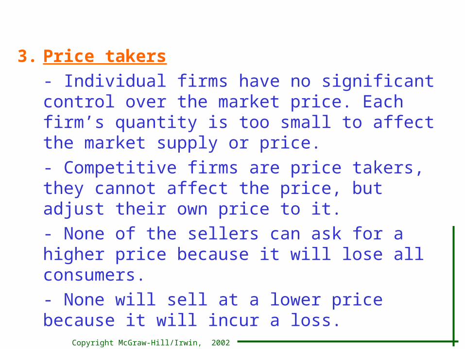
3. Price takers

- Individual firms have no significant control over the market price. Each firm’s quantity is too small to affect the market supply or price.

- Competitive firms are price takers, they cannot affect the price, but adjust their own price to it.

- None of the sellers can ask for a higher price because it will lose all consumers.

- None will sell at a lower price because it will incur a loss.


4. Free entry and exit• New firms can freely enter and existing firms can

freely leave the market.• No significant legal, technological, financial, or other

obstacles prohibit new firms from selling their output in the market.

Relevance of pure competition• Pure competition is rare.• It is highly relevant, we can learn much about markets

by studying the pure competition model. • It is meaningful as a starting point for discussing price

and output determination.• Useful to compare with other markets with regard to

efficiency, price and output.


RevenueTotal Revenue (TR)• Equals the price times the quantity (TR=P x Q).• Total revenue increases by a constant amount for each

unit sold. Average Revenue (AR)• Revenue per unit sold (AR = TR/Q).• The firm’s demand schedule is its revenue schedule. • Price and average revenue are the same (P=AR).Marginal Revenue (MR)• The change in total revenue due to the change in the

quantity sold by one unit (MR = ΔTR/ Δ Q). • Marginal revenue is constant because price is constant.• Marginal revenue equals the price.


Note

Only in a competitive market:

Price = Average revenue = Marginal revenue


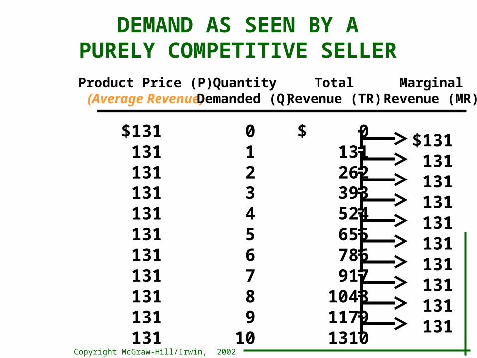
$131 0 $ 0

Product Price (P)(Average Revenue)

TotalRevenue (TR)

MarginalRevenue (MR)

QuantityDemanded (Q)

DEMAND AS SEEN BY APURELY COMPETITIVE SELLER


$131 131

0 1

$ 0131

$131


TotalRevenue (TR)




]


$131 131131

0 1 2

$ 0131262

$131131


TotalRevenue (TR)




]]


$131 131131131

0 1 23

$ 0131262393

$131131131


TotalRevenue (TR)




]]]


$131 131131131131

0 1 234

$ 0131262393524

$131131131131


TotalRevenue (TR)




]]]]


$131 131131131131131131131131131131

0 1 23456789

10

$ 0131262393524655786917

104811791310

$131131131131131131131131131131


TotalRevenue (TR)




]]]]]]]]]]


Perfectly elastic demand

• A firm cannot obtain a higher price by restricting its output, nor does it need to lower its price to increase its sales volume.

• Demand curve faced by the individual competitive firm is perfectly elastic at the market price

• Note that competitive market demand curve is a downward sloping curve.


DEMAND, MARGINAL REVENUE, AND TOTALREVENUE IN PURE COMPETITION

TR

D = MR

1 2 3 4 5 6 7 8 9 10

1179

1048

917

786

655

524

393

262

131

0

Pri

ce

an

d r

ev

enu

e

Quantity Demanded (sold)


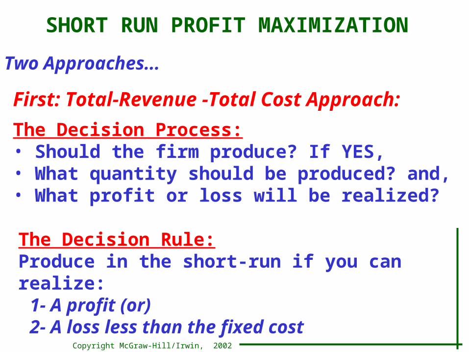
SHORT RUN PROFIT MAXIMIZATION

Two Approaches...

First: Total-Revenue -Total Cost Approach:

The Decision Rule:Produce in the short-run if you can realize:

1- A profit (or)2- A loss less than the fixed cost

The Decision Process:• Should the firm produce? If YES,• What quantity should be produced? and,• What profit or loss will be realized?


TotalCost

0 1 23456789

10

TotalProduct

TotalFixedCost

TotalVariable

CostTotal

Revenue Profit

$ 100 100 100100100100100100100100100

$ 090

170240300370450540649780930

$ 100190270340400470550640749880

1030

Price: $131

- $100- 59

- 8+ 53

+ 124+ 185+ 236+ 277+ 299+ 299+ 280

TOTAL REVENUE-TOTAL COST APPROACH

$ 0131262393524655786917

104811791310

Can you see the

profit maxim

ization?


TotalCost

0 1 23456789

10

TotalProduct

TotalFixedCost

TotalVariable

CostTotal

Revenue Profit

$ 100 100 100100100100100100100100100

$ 090

170240300370450540649780930

$ 100190270340400470550640749880

1030

Price: $131

- $100- 59

- 8+ 53

+ 124+ 185+ 236+ 277+ 299+ 299+ 280


$ 0131262393524655786917

104811791310

Graphing Total

Cost & Revenue


$1,8001,7001,6001,5001,4001,3001,2001,1001,000 900 800 700 600 500 400 300 200 100 0

To

tal r

eve

nu

e a

nd

to

tal c

ost

TotalRevenue

TotalCost

MaximumEconomic

Profits$299

Break-Even Point(Normal Profit)

Break-Even Point(Normal Profit)

1 2 3 4 5 6 7 8 9 10 11 12 13 14



SHORT RUN PROFIT MAXIMIZATIONTwo Approaches...

First: Total-Revenue -Total Cost Approach

Three Characteristics:• The rule applies only if producing is preferred to

shutting down (otherwise the firm will shut down)

• Rule applies to all markets• Rule can be restated as: P=MC

Second Approach:Marginal-Revenue Marginal-Cost Approach

MR = MC Rule


MR = MC rule

In the short run, the firm will maximize profit or

minimize losses by producing the output at which

marginal revenue equals marginal cost.


AverageTotalCost

0 1 23456789

10

TotalProduct

AverageFixedCost

AverageVariable

Cost

Price =MarginalRevenue

TotalEconomicProfit/Loss

$100.00

50.00 33.3325.0020.0016.6714.2912.5011.1110.00

$90.0085.0080.0075.0074.0075.0077.1481.2586.6793.00

$190.00135.00113.33100.00

94.0091.6791.4393.7597.78

103.00

- $100- 59

- 8+ 53

+ 124+ 185+ 236+ 277+ 299+ 299+ 280

MARGINAL REVENUE-MARGINAL COST APPROACH

$ 131131131131131131131131131131

MarginalCost

90807060708090

110131150

Thesame profitmaximizing

result!


AverageTotalCost

0 1 23456789

10

TotalProduct

AverageFixedCost

AverageVariable

Cost

Price =MarginalRevenue

TotalEconomicProfit/Loss

$100.00

50.00 33.3325.0020.0016.6714.2912.5011.1110.00

$90.0085.0080.0075.0074.0075.0077.1481.2586.6793.00

$190.00135.00113.33100.00

94.0091.6791.4393.7597.78

103.00

- $100- 59

- 8+ 53

+ 124+ 185+ 236+ 277+ 299+ 299+ 280


$ 131131131131131131131131131131

MarginalCost

90807060708090

110131150


Two Ways to Calculate Profit

First: Calculate total profit

TR = P x Q

TC = ATC x Q

Π = TR – TC

Second: calculate profit per unitΠ /Q = TR/Q – TC/QΠ /Q = P (or AR) – ATC Π = (Π /Q) x Q


$200

150

100

50

0

Co

st a

nd

Rev

enu

e

1 2 3 4 5 6 7 8 9 10

MC

MR

AVCATC

Economic Profit

$131.00

$97.78


Profit Maximization Position


$200

150

100

50

0

Co

st a

nd

Rev

enu

e

1 2 3 4 5 6 7 8 9 10

MC

MR

AVCATC

Economic Profit

$131.00

$97.78


MR = MCOptimumSolution

Profit Maximization Position


The MR=MC rule still applies

If the price is lowered from $131 to $81

…But the MR = MC point changes

Note: π = π per unit x Q


Loss Minimization Position


$200

150

100

50

0

Co

st a

nd

Rev

enu

e

1 2 3 4 5 6 7 8 9 10

MC

MRAVCATC

Economic Loss

$81.00$91.67


Loss Minimization Position


$200

150

100

50

0

Co

st a

nd

Rev

enu

e

1 2 3 4 5 6 7 8 9 10

MC

MR

AVCATC

$71.00

Short-Run Shut Down Point

Minimum AVCis the Shut-Down

Point



Marginal Cost & Short-Run Supply

PriceQuantitySupplied

Maximum Profit (+)Or Minimum Loss (-)

Observe the impact upon profitability as price is changed

$151 131 111 91 81 71 61

10987600

$+480+299

+138 -3

-64 -100 -100



Co

st a

nd

Rev

enu

e, (

do

llar

s) MC

MR1

AVC

ATC

Quantity Supplied

MR2

MR3

MR4

MR5

P1

P2

P3

P4

P5

Q2 Q3 Q4 Q5


Do notProduce –

Below AVC



Co

st a

nd

Rev

enu

e, (

do

llar

s)MC

MR1

Quantity Supplied

MR2

MR3

MR4

MR5

P1

P2

P3

P4

P5

Q2 Q3 Q4 Q5

Marginal Cost & Short-Run SupplyYields theShort-Run

Supply Curve

Supply

NoProductionBelow AVC




AVC2

MC2

Higher Costs Move theSupply Curve to the LeftC

ost

an

d R

even

ue,

(d

oll

ars)

MC1

AVC1

Quantity Supplied

S1

S2




AVC2

MC2

Lower Costs Movethe Supply Curve

to the Right

Co

st a

nd

Rev

enu

e, (

do

llar

s)MC1

AVC1

Quantity Supplied

S1

S2



P

Q

S=MC

AVC

ATC

8

D

P

Q8000

D

S= MC’s

IndustryFirm(price taker)

EconomicProfit

$111$111

SHORT RUN COMPETITIVE EQUILIBRIUMThe Competitive Firm “Takes” its Price from the Industry Equilibrium


P

Q

S=MC

AVC

ATC

8

D

P

Q8000

D

S= MC’s


EconomicProfit

$111$111

SHORT RUN COMPETITIVE EQUILIBRIUMThe Competitive Firm “Takes” it’s Price from the Industry Equilibrium


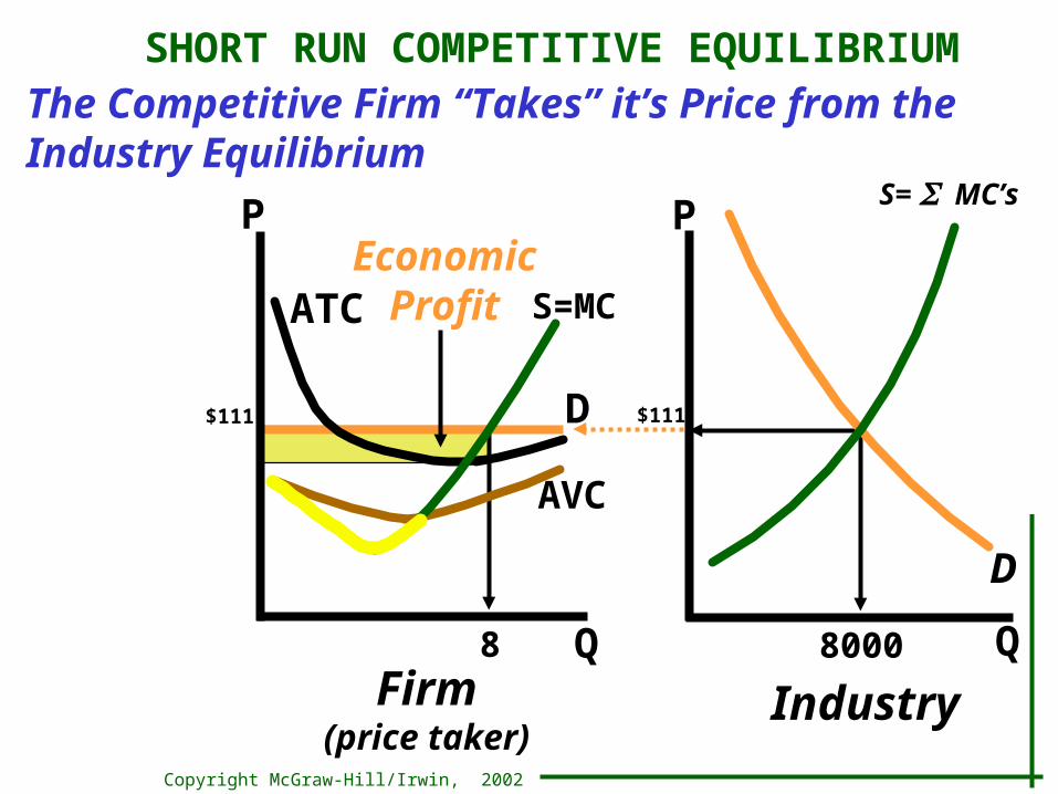
PROFIT MAXIMIZATION IN THE LONG-RUN

Assumptions...• Entry and Exit Only: the only long run adjustment is the entry and exit of firms. • Identical Costs: all firms in the industry have identical cost curves.• Constant-Cost Industry: entry and exit does not affect resource prices.

Goal...Price = Minimum ATC

Zero Economic Profit Model


Temporary Profits and the Reestablishment Of Long-Run Equilibrium

S1

MCATC

P

Q100

P

Q100,000


$60

50

40

$60

50

40


MR

D1


An increase in demand increases profits…

MR

D1

MCATC

P

Q100

P

Q100,000


$60

50

40

$60

50

40


D2

EconomicProfits

S1


New Competitors increase supply and lower Prices decrease economic profits

MR

D1

MCATC

P

Q100

P

Q100,000


$60

50

40

$60

50

40


D2

Zero EconomicProfits

S1

S2


Decreases in demand, Losses and the Reestablishment of Long-Run Equilibrium

S1

MCATC

P

Q100

P

Q100,000


$60

50

40

$60

50

40


D1

MR


A decrease in demand creates losses…

MR

D1

MCATC

P

Q100

P

Q100,000


$60

50

40

$60

50

40


D2

EconomicLosses

S1


MR

D1

MCATC

P

Q100

P

Q100,000


$60

50

40

$60

50

40


D2

Return to ZeroEconomic Profits

S1

S3

Competitors with losses decrease supply and prices return to zero economic profits


LONG-RUN SUPPLY IN ACONSTANT COST INDUSTRY

Constant Cost Industry

Perfectly Elastic Long-Run Supply: entry and exit will set the price back to its original level

Graphically...


P

Q

=$50 S

D1

Z1

Q1

D2

Z2

Q2Q3

D3

Z3

100,000 110,00090,000

LONG-RUN SUPPLY IN ACONSTANT COST INDUSTRY

P1

P2

P3


P

Q

$555045

S

D1

Y1

Q1

D2

Y2

Q2Q3

D3

Y3

100,000 110,00090,000

LONG-RUN SUPPLY IN ANINCREASING COST INDUSTRY

P1

P2

P3


P

Q

$555045

S

D1

Y1

Q1

D2

Y2

Q2Q3

D3

Y3

100,000 110,00090,000

P1

P2

P3

LONG-RUN SUPPLY IN ANINCREASING COST INDUSTRY


P MR

Q

MCATC

Quantity

Pri

ce

Price = MC = Minimum ATC(normal profit)

LONG-RUN EQUILIBRIUM FOR A COMPETITIVE FIRM


PURE COMPETITION AND EFFICIENCY

Productive Efficiency: Price = Minimum ATC

Allocative Efficiency: Price = MC

Underallocation: Price > MC

Overallocation: Price < MC

Resources are efficiently allocated

Under pure competition

copyright mcgraw-hill/irwin, 2002 chapter 23: pure competition

Documents