This is an electronic reprint of the original article.This reprint may differ from the original in pagination and typographic detail.

Powered by TCPDF (www.tcpdf.org)

This material is protected by copyright and other intellectual property rights, and duplication or sale of all or part of any of the repository collections is not permitted, except that material may be duplicated by you for your research use or educational purposes in electronic or print form. You must obtain permission for any other use. Electronic or print copies may not be offered, whether for sale or otherwise to anyone who is not an authorised user.

Susi, T.; Kaukonen, M.; Havu, P.; Ljungberg, M.P.; Ayala, P.; Kauppinen, E.I.Core level binding energies of functionalized and defective graphene

Published in:Beilstein Journal of Nanotechnology

DOI:10.3762/bjnano.5.12

Published: 01/01/2014

Document VersionPublisher's PDF, also known as Version of record

Published under the following license:CC BY

Please cite the original version:Susi, T., Kaukonen, M., Havu, P., Ljungberg, M. P., Ayala, P., & Kauppinen, E. I. (2014). Core level bindingenergies of functionalized and defective graphene. Beilstein Journal of Nanotechnology, 5, 121-132.https://doi.org/10.3762/bjnano.5.12

121

Core level binding energies of functionalizedand defective graphene

Toma Susi*1,2, Markus Kaukonen1,3, Paula Havu1,4, Mathias P. Ljungberg5,Paola Ayala2 and Esko I. Kauppinen1

Full Research Paper Open Access

Address:1Department of Applied Physics, Aalto University School of Science,PO Box 15100, FI-00076 Aalto, Finland, 2University of Vienna,Faculty of Physics, Strudlhofgasse 4, A-1090 Vienna, Austria),3Present address: Helsingin matematiikkalukio, Kuusikkotie 3, 00630Helsinki, Finland, 4Present address: Suomen ympäristökeskus,Mechelininkatu 34a, 00260 Helsinki, Finland and 5LOMA, UniversitéBordeaux 1, 351 Cours de la Libération, 33405 Talence, France

Email:Toma Susi* - toma.susi@iki.fi

* Corresponding author

Keywords:core level; defects; density functional theory; graphene; X-rayphotoelectron spectroscopy

Beilstein J. Nanotechnol. 2014, 5, 121–132.doi:10.3762/bjnano.5.12

Received: 15 October 2013Accepted: 17 January 2014Published: 03 February 2014

This article is part of the Thematic Series "Physics, chemistry and biologyof functional nanostructures II".

Guest Editor: A. S. Sidorenko

© 2014 Susi et al; licensee Beilstein-Institut.License and terms: see end of document.

AbstractX-ray photoelectron spectroscopy (XPS) is a widely used tool for studying the chemical composition of materials and it is a stan-

dard technique in surface science and technology. XPS is particularly useful for characterizing nanostructures such as carbon nano-

materials due to their reduced dimensionality. In order to assign the measured binding energies to specific bonding environments,

reference energy values need to be known. Experimental measurements of the core level signals of the elements present in novel

materials such as graphene have often been compared to values measured for molecules, or calculated for finite clusters. Here we

have calculated core level binding energies for variously functionalized or defected graphene by delta Kohn–Sham total energy

differences in the real-space grid-based projector-augmented wave density functional theory code (GPAW). To accurately model

extended systems, we applied periodic boundary conditions in large unit cells to avoid computational artifacts. In select cases, we

compared the results to all-electron calculations using an ab initio molecular simulations (FHI-aims) code. We calculated the carbon

and oxygen 1s core level binding energies for oxygen and hydrogen functionalities such as graphane-like hydrogenation, and

epoxide, hydroxide and carboxylic functional groups. In all cases, we considered binding energy contributions arising from carbon

atoms up to the third nearest neighbor from the functional group, and plotted C 1s line shapes by using experimentally realistic

broadenings. Furthermore, we simulated the simplest atomic defects, namely single and double vacancies and the

Stone–Thrower–Wales defect. Finally, we studied modifications of a reactive single vacancy with O and H functionalities, and

compared the calculated values to data found in the literature.

121

Beilstein J. Nanotechnol. 2014, 5, 121–132.

122

IntroductionX-ray photoelectron spectroscopy (XPS) is commonly used to

identify the relative amounts of chemical elements in a sample,

and it can provide information about their chemical states, i.e.,

bonding. Although the method is not local, XPS is able to

discern specific atomic defects if they are numerous enough

and, furthermore, provide essential statistical information on

their concentrations. Typically, XPS has been limited to surface

characterization because of the limited escape depth of

photoemitted electrons. However, for low-dimensional carbon

nanomaterials such as graphene or carbon nanotubes, the escape

depth exceeds the size of the system, and this makes XPS in

practice a convenient bulk characterization tool.

In order to interpret the binding energies measured by XPS, a

reference to which such energies can be compared is needed.

Density functional theory (DFT) calculations can be employed

to provide such a reference, especially when measurements of

known molecular systems are not sufficient. However, because

of the computational cost of treating core levels accurately,

most calculations up to date have considered either non-peri-

odic (cluster-type) systems or small unit cells. This has made

the simulation of extended defects challenging and subject to

questionable approximations, and possibly even spurious

image–image interaction or finite size effects. Furthermore,

the electronic structure of molecular models such as

coronenes differs significantly from graphene, which can be an

issue.

A prominent recent example of the value of XPS for studying

graphene is in chemical functionalization, in which the pristine

structure is modified by a known covalent adsorbate or a substi-

tution. Besides substitutional doping, which we will not discuss

here, the functionalization of graphene by, e.g., hydrogenation

[1,2] and oxygenation [3,4] has been a topic of intense research.

These treatments result in –H, –O, or –OH groups bonded to the

carbon atoms, the orbital hybridization of which is changed

from sp2 to sp3. This can lead to a band gap opening [3] and

other interesting features [5]. To study such functional groups,

along with intrinsic defects, is also vital for the spectroscopic

analysis of reduced graphene oxide [6,7], which in turn is a

promising avenue to the mass production of graphene.

Several intrinsic defects are relevant for graphene. Of these, the

simplest are single (SV) and double vacancies (DV), along with

the Stone–Thrower–Wales (STW) bond rotation. All of these

have been directly observed [8] in aberration-corrected trans-

mission electron microscopes (TEM). More extended defects

(such as the 555-777 and the 5555-6-7777 double vacancy

defects [9]) have also been seen, but are likely to be beam-

induced. In any case, locally they do not present very different

bonding environments, and thus their XPS signatures are

unlikely to differ significantly from the simpler cases.

The single vacancy is different from the DV (called V2(5-8-5)

by Banhart et al. [9]) and the STW (SW(555-777) [9]) as by

necessity it presents dangling bonds. The removal of a single

carbon atom from a graphene lattice leaves the three neigh-

boring atoms with a single dangling bond each, which can be

called an unreconstructed single vacancy (uSV). As this is

energetically unfavorable, two of the atoms tend to form a

bond between themselves and reconstruct to close a pentagon

[8] in the Jahn–Teller distortion [10]. We will call this a recon-

structed single vacancy, or simply SV (V1(5-9) [9]). However,

the remaining single carbon atom still cannot satisfy its

chemically reactive dangling bond, as has been directly

observed by scanning tunneling microscopy (STM) in high

vacuum [11].

To address these important systems, and the potential short-

comings of previous studies, we have calculated graphene core

level binding energies by using density functional theory imple-

mented with real-space grid-based projector-augmented waves

in the GPAW code [12]. We applied periodic boundary condi-

tions in large unit cells to avoid spurious image interaction

effects. Furthermore, we benchmarked select results against all-

electron calculations with the FHI-aims code [13] to ensure that

the projector-augmented waves in GPAW described the core

levels of these systems accurately.

In addition to pristine graphene, we studied hydrogen (-H),

dihydrogen (2 –H), graphane-like dihydrogen (2 –Hopp, i.e., two

neighboring H adatoms on opposite sides of the graphene sheet

[2]) hydroxide (–OH), oxygen (=O), dioxygen (–2O), epoxide

(>O, [3,4]), and carboxylic (–COOH, [14]) functional groups.

The defect structures we studied were the single vacancy (SV),

double vacancy (DV) and the Stone–Thrower–Wales (STW)

defects. Several modifications of the SV site were considered as

well, as the dangling bond constitutes a reactive site for the

absorption of molecules from the environment. As the absorp-

tion of more electronegative atoms can have a large impact on

the C 1s binding energy of the neighboring carbon atom, the

following adsorbates were considered: hydrogen (SV–H),

ketone (SV=O), annulene (SV–O–, [15]), ketone + annulene

(SV=O+–O–), diketone (SV=2O, possibly relevant for oxygen

splitting [16]), hydroxide (SV–OH), and carboxylic

(SV–COOH) groups.

We found that the projector-augmented results were in excel-

lent agreement with all-electron calculations. In almost all

cases, in which data was available, a good agreement for the

Beilstein J. Nanotechnol. 2014, 5, 121–132.

123

Figure 1: a) The 9 × 9 graphene computational unit cell. Cropped relaxed structures of the b) reconstructed single vacancy (SV), c) the doublevacancy (DV), and d) the Stone–Thrower–Wales (STW) defect.

C 1s levels with experimental values reported in the literature

was also found [4,17-20]. As a further refinement, we consid-

ered binding energy contributions arising from up to third

nearest neighbors to the functional group or defect, and plotted

the resulting line shapes by using experimentally realistic

broadenings. In the case of the O 1s level, the line-shape varia-

tions of graphene have not been extensively examined in

experimental reports, which makes the comparison of the calcu-

lated O 1s values to literature data problematic. This is why we

have focused our discussion on the C 1s energies. With this

caveat, core-hole calculations with the GPAW code are a con-

venient and valuable tool for simulating the core level binding

energies of graphene systems.

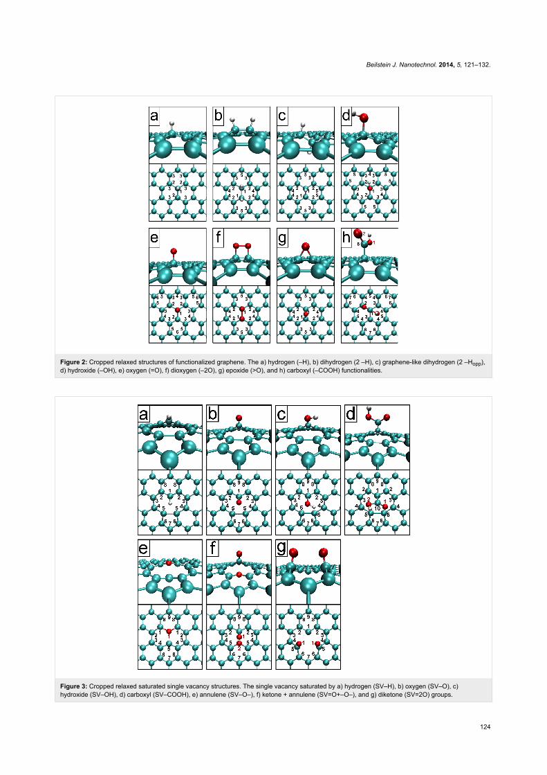
ResultsRelaxed structuresThe relaxed structures are shown in Figure 1, Figure 2, and

Figure 3. Note that all systems were allowed to relax with no

constraints, which induced a slight curvature into some of the

structures to compensate for the strain induced by the local

defects. The unreconstructed single vacancy spontaneously

reconstructed during the geometry relaxation, by closing a

pentagonal carbon ring. The bond lengths and angles of the

relaxed structures match closely to what has been reported in

the literature [3,4,9,14,16]. The Arabic numerals denote the

target atoms of the core-hole calculations discussed below.

Formation energiesThe formation energies of the defects were calculated according

to Equation 1, found in section “Computational details“ below

along with the chemical potentials chosen for the missing

carbon atoms and the added functional groups. The formation

energy of the STW defect was calculated to be 4.99 eV, in

perfect agreement with previous studies [2]. The values for the

single (7.21 eV) and double vacancies (7.01 eV) are marginally

lower than previously reported, which could be attributed to the

unconstrained structural relaxation allowed here. Following

Banhart et al. [9], it should be noted that the formation energy

per atom is much lower for the double vacancy.

The formation energies of the saturated vacancy structures were

calculated with respect to the bare single vacancy. The hydro-

Beilstein J. Nanotechnol. 2014, 5, 121–132.

124

Figure 2: Cropped relaxed structures of functionalized graphene. The a) hydrogen (–H), b) dihydrogen (2 –H), c) graphene-like dihydrogen (2 –Hopp),d) hydroxide (–OH), e) oxygen (=O), f) dioxygen (–2O), g) epoxide (>O), and h) carboxyl (–COOH) functionalities.

Figure 3: Cropped relaxed saturated single vacancy structures. The single vacancy saturated by a) hydrogen (SV–H), b) oxygen (SV–O), c)hydroxide (SV–OH), d) carboxyl (SV–COOH), e) annulene (SV–O–), f) ketone + annulene (SV=O+–O–), and g) diketone (SV=2O) groups.

Beilstein J. Nanotechnol. 2014, 5, 121–132.

125

genated SV had a formation energy of −2.46 eV due to the satu-

ration of the dangling bond. The lowest formation energies were

obtained for the oxygen-saturated structures, with the ketone-

saturated (SV=O) vacancy at −4.01 eV, the diketone (=2O) at

−4.91 eV, the annulene-bridged vacancy (SV-O-) at –4.00 eV,

and finally, the annulene plus ketone vacancy structure

(SV=O + -O-), which had by far the lowest value at −8.65 eV.

In agreement with a previous calculation, which used a cluster

model [14], the carboxyl-saturated vacancy (SV-COOH) has a

formation energy −1.62 eV compared to the SV, or 3.12 eV

compared to the pristine structure.

The formation energies of the functional groups without vacan-

cies are 1.45 eV for the -H adatom (in good agreement with a

previous calculation [21]), 1.70 eV for 2 -H, 2.30 eV for the

-OH, 1.20 eV for the =O, 0.74 eV for adjacent =O adatoms, and

2.07 eV for the carboxylic group -COOH. The epoxide group

>O had a remarkably low formation energy of 0.3 eV, in line

with the thermally reversible oxidation recently observed exper-

imentally by Hossain and co-workers [4].

Core level binding energiesThe core level binding energies were calculated according to the

delta Kohn–Sham total energy differences method [22,23] as

detailed in section “Computational details”. The calculated core

level binding energies for the pristine and defected graphene are

shown in Table 1, for functionalized graphene in Table 2, and

for the saturated vacancy configurations in Table 3. C(*)

denotes a carbon atom far away from the defect (“bulk”), and

“*” in the column “# of atoms” denotes that the number of such

atoms depends on the defect concentration. For each configur-

ation, we calculated the C 1s binding energies (and O 1s, where

applicable) for up to third nearest neighbor C atoms from the

defect to capture the significant shifts while keeping the compu-

tational effort manageable. Target atoms are denoted by Arabic

numerals in Figures 1–3 with the same numeral denoting

multiple equivalent atoms, and the number of atoms of each

type is noted in Tables 1–3.

For the all-electron FHI-aims calculations, we considered the

pristine, SV, -H, and 2 -Hopp configurations. Although the C 1s

energy of pristine graphene had a slightly different absolute

value with FHI-aims (283.69 eV vs 283.61 eV), the all-electron

calculations gave binding energy shifts within 10 meV of the

GPAW results. This demonstrates that the use projector-

augmented waves in the GPAW calculations is not a significant

source of error.

Line shapesTo help interpret the calculated core level binding energies

shown in Tables 1–3, we plotted line shapes for each configur-

Table 1: Calculation results for the pristine and defected graphenestructures. The columns show: system identifier; formation energy ofthe defect; target atom of the calculation (see Figure 1); number oftarget atoms; calculated 1s binding energy; C 1s BE shift with respectto the calculated C 1s energy of pristine graphene.

ID Eform(eV)

atom # ofatoms

C 1s BE(eV)

BE shift(eV)

gra 0 C (*) * 283.61 0.00

SV 7.21 C (*) * 283.32 −0.29C (1) 1 281.21 −2.40C (2) 2 282.97 −0.64C (3) 2 282.87 −0.74C (4) 2 283.55 −0.06C (5) 2 283.24 −0.37C (6) 2 292.91 −0.70C (7) 1 282.51 −1.10C (8) 2 282.97 −0.64

DV 7.02 C (*) * 283.39 −0.22C (1) 4 283.27 −0.34C (2) 4 282.79 −0.82C (3) 4 283.58 −0.03C (4) 2 282.43 −1.18C (5) 4 283.53 −0.08C (6) 4 283.21 −0.40C (7) 2 283.12 −0.49

S-W 4.99 C (*) * 283.61 0.00C (1) 2 283.10 −0.51C (2) 4 283.16 −0.45C (3) 4 283.83 0.22C (4) 4 282.67 −0.94C (5) 2 283.70 0.09C (6) 4 283.27 −0.34

Table 2: Calculation results for the functionalized graphene structures.The columns show: system identifier; formation energy of the defect;target atom of the calculation (see Figure 2); number of target atoms;calculated 1s binding energy; C 1s BE shift with respect to the calcu-lated C 1s energy of pristine graphene or the O 1s BE shift withrespect to the calculated O 1s energy of epoxide/hydroxide functionalgroups, where applicable.

ID Eform(eV)

atom # ofatoms

1s BE(eV)

BE shift(eV)

gra 0 C (*) * 283.61 0.00

-H 1.45 C (*) * 283.39 −0.22C (1) 1 284.10 0.49C (2) 3 282.78 −0.83C (3) 6 283.35 −0.26

2 -H 1.69 C (*) * 283.59 −0.02

Beilstein J. Nanotechnol. 2014, 5, 121–132.

126

Table 2: Calculation results for the functionalized graphene structures.The columns show: system identifier; formation energy of the defect;target atom of the calculation (see Figure 2); number of target atoms;calculated 1s binding energy; C 1s BE shift with respect to the calcu-lated C 1s energy of pristine graphene or the O 1s BE shift withrespect to the calculated O 1s energy of epoxide/hydroxide functionalgroups, where applicable. (continued)

C (1) 2 284.55 0.94C (2) 4 283.19 −0.42C (3) 4 283.58 −0.03C (4) 4 283.55 −0.05C (5) 2 283.31 −0.30

2 -Hopp 1.30 C (*) * 283.59 −0.02C (1) 2 284.36 0.75C (2) 4 283.16 −0.45C (3) 4 283.60 −0.01C (4) 4 283.53 −0.08C (5) 2 283.31 −0.30

-OH 2.30 C (*) * 283.38 −0.23C (1) 1 284.81 1.20C (2) 3 282.35 −1.26C (3) 6 282.91 −0.70C (4) 3 282.83 −0.78C (5) 6 283.29 −0.02

O 1 530.11 0.00

=O 1.20 C (*) * 283.38 −0.23C (1) 1 283.93 0.32C (2) 3 282.35 −1.25C (3) 6 282.91 −0.70C (4) 3 282.83 −0.78C (5) 6 283.14 −0.47C (6) 3 283.16 −0.45

O 1 526.36 −3.75

-2O 0.74 C (*) * 283.53 −0.08C (1) 2 285.16 1.55C (2) 4 283.00 −0.61C (3) 4 283.44 −0.17C (4) 4 283.45 −0.16C (5) 2 282.83 −0.78

O 2 530.29 0.18

>O 0.29 C (*) * 283.57 −0.04C (1) 2 285.13 1.52C (2) 4 283.16 −0.45C (3) 4 283.56 −0.05C (4) 4 283.55 −0.07C (5) 2 283.30 −0.31

O 1 530.11 0.00

-COOH 2.07 C (*) * 283.34 −0.27C (1) 1 284.43 0.81C (2) 1 282.67 −0.94

Table 2: Calculation results for the functionalized graphene structures.The columns show: system identifier; formation energy of the defect;target atom of the calculation (see Figure 2); number of target atoms;calculated 1s binding energy; C 1s BE shift with respect to the calcu-lated C 1s energy of pristine graphene or the O 1s BE shift withrespect to the calculated O 1s energy of epoxide/hydroxide functionalgroups, where applicable. (continued)

C (3) 2 282.77 −0.84C (4) 6 283.21 −0.40C (5) 3 282.89 −0.72C (6) 6 282.26 −0.35C (7) 3 283.36 −0.25C (8) 1 286.07 2.46O (1) 1 532.82 2.71O (2) 1 530.50 0.39

Table 3: Calculation results for the saturated single vacancy struc-tures. The columns show: system identifier; formation energy of thedefect; target atom of the calculation (see Figure 3); number of targetatoms; calculated 1s binding energy; C 1s BE shift with respect to thecalculated C 1s energy of pristine graphene or the O 1s BE shift withrespect to the calculated O 1s energy of epoxide/hydroxide functionalgroups, where applicable.

ID Eform(eV)

atom # ofatoms

1s BE(eV)

BE shift(eV)

SVa 0 — — — —

SV-H −2.46 C (*) * 283.30 −0.31C (1) 1 282.11 −1.50C (2) 2 283.00 −0.61C (3) 2 282.96 −0.65C (4) 2 283.65 0.04C (5) 2 283.24 −0.37C (6) 2 282.78 −0.83C (7) 1 282.37 −0.24C (8) 2 283.09 −0.52

SV=O −4.01 C (*) * 283.47 −0.14C (1) 1 284.27 0.65C (2) 2 282.64 −0.97C (3) 2 283.27 −0.34C (4) 2 283.65 0.04C (5) 2 283.42 −0.19C (6) 2 283.01 −0.60C (7) 1 282.60 −1.01C (8) 2 283.26 −0.35C (9) 1 283.05 −0.56

O 2 528.88 −1.23

SV-OH −1.53 C (*) * 283.35 −0.26C (1) 1 284.03 0.42C (2) 2 282.98 −0.63C (3) 2 283.03 −0.58

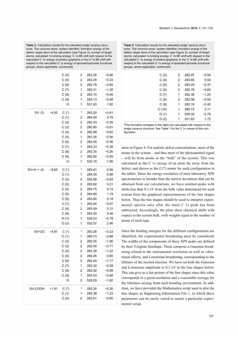
Beilstein J. Nanotechnol. 2014, 5, 121–132.

127

Table 3: Calculation results for the saturated single vacancy struc-tures. The columns show: system identifier; formation energy of thedefect; target atom of the calculation (see Figure 3); number of targetatoms; calculated 1s binding energy; C 1s BE shift with respect to thecalculated C 1s energy of pristine graphene or the O 1s BE shift withrespect to the calculated O 1s energy of epoxide/hydroxide functionalgroups, where applicable. (continued)

C (4) 2 283.55 −0.06C (5) 2 283.28 −0.33C (6) 2 282.79 −0.82C (7) 1 282.41 −1.20C (8) 2 283.15 −0.46C (9) 1 283.13 −0.48

O 1 531.93 1.82

SV -O- −4.00 C (*) * 283.20 −0.41C (1) 2 284.40 0.79C (2) 2 283.33 −0.28C (3) 2 282.80 −0.81C (4) 2 282.99 −0.62C (5) 1 281.25 −2.06C (6) 2 283.05 −0.56C (7) 1 283.23 −0.38C (8) 2 283.35 −0.26C (9) 1 282.92 −0.59

O 1 532.10 1.99

SV=O + -O- −8.65 C (*) * 283.61 0.00C (1) 1 284.59 0.98C (2) 2 282.98 −0.63C (3) 2 283.62 0.01C (4) 2 283.75 0.14C (5) 2 284.89 1.19C (6) 2 283.80 0.19C (7) 1 283.54 −0.07C (8) 2 283.49 0.12C (9) 1 283.25 0.36O (1) 1 529.23 −0.78O (2) 1 532.57 2.46

SV=2O −4.91 C (*) * 283.28 −0.33C (1) 1 280.73 −2.88C (2) 2 282.55 −1.06C (3) 2 282.90 −0.71C (4) 2 282.39 −1.22C (5) 2 284.26 0.65C (6) 2 282.44 −1.17C (7) 1 283.32 −0.29C (8) 2 282.92 −0.69C (9) 1 283.03 −0.58

O 2 528.29 −1.82

SV-COOH −1.61 C (*) * 283.35 −0.26C (1) 1 282.38 −1.23C (2) 2 283.01 −0.60

Table 3: Calculation results for the saturated single vacancy struc-tures. The columns show: system identifier; formation energy of thedefect; target atom of the calculation (see Figure 3); number of targetatoms; calculated 1s binding energy; C 1s BE shift with respect to thecalculated C 1s energy of pristine graphene or the O 1s BE shift withrespect to the calculated O 1s energy of epoxide/hydroxide functionalgroups, where applicable. (continued)

C (3) 2 282.97 −0.64C (4) 2 283.65 0.04C (5) 2 283.24 −0.37C (6) 2 282.79 −0.82C (7) 1 282.36 −1.25C (8) 2 283.08 −0.53C (9) 1 283.19 −0.42

C (10) 1 285.72 2.11O (1) 1 529.32 −0.79O (2) 1 531.83 1.72

aThe formation energies in this table are calculated with respect to thesingle vacancy structure. See Table 1 for the C 1s values of this con-figuration.

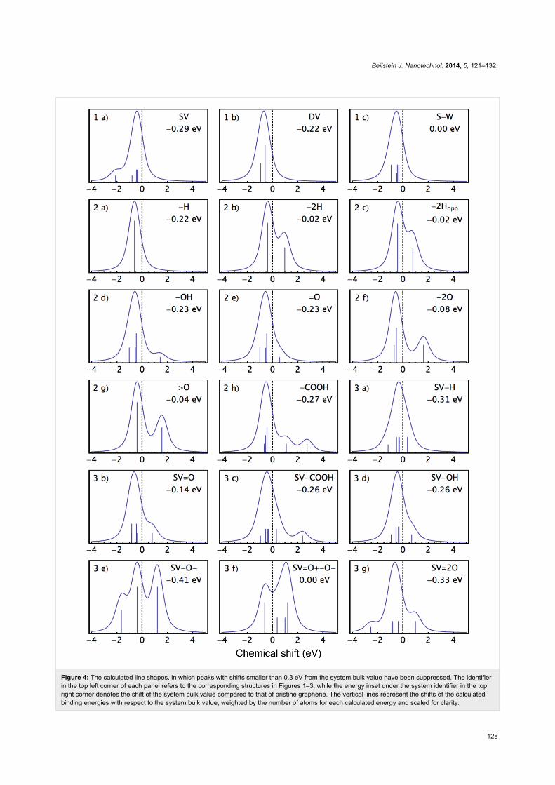
ation in Figure 4. For realistic defect concentrations, most of the

atoms in the system – and thus most of the photoemitted signal

– will be from atoms in the “bulk” of the system. This was

calculated as the C 1s energy of an atom far away from the

defect, and shown as the C(*) atoms for each configuration in

the tables. Since the energy resolution of most laboratory XPS

spectrometers is broader than the narrow deviations that can be

obtained from our calculations, we have omitted peaks with

shifts less than 0.3 eV from the bulk value determined for each

system from the graphical representations of the line shapes

below. Thus the line shapes should be used to interpret experi-

mental spectra only after the main C 1s peak has been

subtracted. Accordingly, the plots show chemical shifts with

respect to the system bulk, with weights equal to the number of

atoms of each type.

Once the binding energies for the different configurations are

identified, the experimental broadening must be considered.

The widths of the components of these XPS peaks are defined

by their Voigtian lineshape. These comprise a Gaussian broad-

ening related to the instrumental resolution as well as vibra-

tional effects, and Lorentzian broadening, corresponding to the

lifetime of the excited electron. We have set both the Gaussian

and Lorentzian amplitude to 0.3 eV in the line shapes below.

This can give us a fair picture of the line shapes since this value

corresponds to a good resolution and a reasonable average for

the lifetimes arising from each bonding environment. In add-

ition, we have provided the Mathematica script used to plot the

line shapes as Supporting Information File 1, in which these

parameters can be easily varied to match a particular experi-

mental setup.

Beilstein J. Nanotechnol. 2014, 5, 121–132.

128

Figure 4: The calculated line shapes, in which peaks with shifts smaller than 0.3 eV from the system bulk value have been suppressed. The identifierin the top left corner of each panel refers to the corresponding structures in Figures 1–3, while the energy inset under the system identifier in the topright corner denotes the shift of the system bulk value compared to that of pristine graphene. The vertical lines represent the shifts of the calculatedbinding energies with respect to the system bulk value, weighted by the number of atoms for each calculated energy and scaled for clarity.

Beilstein J. Nanotechnol. 2014, 5, 121–132.

129

DiscussionThe value of the carbon 1s core level binding energy of graphite

is commonly cited to be at 284.4 eV [18,24]. In the case of

graphene, however, this value varies according to the substrate,

on which graphene is placed or grown. Some authors have

measured the C 1s of epitaxial monolayered graphene at a

slightly higher value of 284.8 eV, but attribute this to a charge

transfer from the SiC substrate [25]. A similar shift has been

observed for the Dirac point in this system by angle-resolved

photoemission spectroscopy [26]. Other authors have measured

the C 1s at 284.15 eV [27] on Ir(111) and 284.2 eV on Au-inter-

calated Ni(111) [28], but again, charge transfer very likely

contributes to the results. Since no conclusive XPS data on free-

standing monolayered graphene is available so far, we have

chosen to use 284.4 eV as the reference value for the graphene

C 1s binding energy.

Looking at the calculated C 1s value of pristine graphene in Ta-

ble 1, we can see that the computational method underestimates

the binding energy by 0.8 eV. As mentioned above, the absolute

values for the DFT energies will depend on the functional that

was used. Errors on the order of 1 eV compared to the experi-

mental values are typical [23]. A common practice to compare

simulations to experiments is to rigidly shift the calculated

values to match a well-known experimental value, which allows

the prediction of core level binding energies for atomic configu-

rations that are not known experimentally. Thus the experimen-

tally meaningful values are the shifts of the C 1s energy with

respect to the graphene bulk value, which are shown as the last

column of Tables 1–3. However, it should be noted that the

C 1s values for bulk atoms in certain configurations differ from

the pristine graphene value by up to 0.4 eV. This shift depends

on the computational unit cell size and would certainly be

affected by the presence of a substrate. We have thus chosen to

list the absolute shifts with respect to the pristine value in

Tables 1–3, but use the shifted bulk values in the graphical

representations of the line shapes shown above.

First, we must note that the C 1s energies calculated for the

intrinsic defects (SV, DV and STW) are lower than the pristine

graphene energy. This is only rarely seen in experiments,

perhaps because of the spontaneous saturation of such sites

under ambient conditions, as suggested by the negative forma-

tion energies of the saturated SV structures (Table 3). Speranza

et al. [18] measured such negative shifts for irradiated graphite,

and speculated that a component shifted by −0.5 eV could be

due to an imbalance of electric charge around vacancies.

Barinov et al. [17] explicitly calculated the dangling bond atom

in the SV to have a downshift of −1.1 eV, while the two atoms

in the pentagon have shifts of −0.7 eV. Our calculations give

corresponding values of −2.4 and −0.37 eV. However, several

other atoms surrounding the vacancy present shifts of around

−0.7 eV. The binding energies for the DV and the STW defects

present similar downshifts from the pristine value as in the SV

case, but not quite as large.

The calculated values for the functionalized graphene systems

can be found in Table 2. The C 1s value of the carbon atoms

bonded to oxygen in the epoxide configuration (>O) is 1.5 eV

higher than the pristine graphene value, in excellent agreement

with Barinov et al., who calculated a shift of 1.6 eV [17]

(although it should be noted that the experimental shift reported

by Hossain et al. is slightly higher at 1.8 eV [4]). However,

atoms 2 and 5 present negative shifts of −0.45 and −0.31 eV,

respectively, contributing to the overall signature of these

groups. For functionalities without vacancies, commonly

accepted shifts in the literature [19,20] are 1.3–1.7 eV for a

carbon bonded to -OH, 2.5–3.0 eV to =O, and 4.0–4.5 eV to

-COOH. Looking at the values in Table 1, we find 1.2 eV for

-OH, only 0.32 eV for =O, and 2.5 eV for -COOH. We note that

the reference for =O actually comes from benzoquinone, which

has =O functionalities at neighboring sites of the benzene ring.

Thus we also considered a -2O functionality with oxygen atoms

bonded to two adjacent carbon atoms. This gave a C 1s energy

shift of 1.6 eV, which is closer to the literature value. However,

it should be noted that the systems considered in the references

above are different than those considered here, and thus one

should not expect a perfect agreement. Looking at Table 2, we

see that even when the C atom bonded to the functional group

presents a positive shift, this is invariably compensated by nega-

tive shifts on neighboring carbons.

The calculated values for the saturated vacancy systems can be

found in Table 3. For a single vacancy saturated with oxygen

(SV-O), we found a shift of 0.67 eV (smaller than a reported

value of 1.4 eV [17]). For the dangling bond atom in the

hydroxyl group saturated vacancy (SV-OH) the C 1s is shifted

by 0.42 eV, but the carbon atom at the other side of the vacancy

close to the H presents a downshift of −0.29 eV, which is small

but could still be experimentally observable. The carboxylic

group presents large shifts of −1.23 eV for the dangling bond

atom, and +2.11 eV for the carbon bonded to the two oxygens.

However, considering the relatively high formation energies of

the latter two structures, it should be noted that they might not

represent stable ground state configurations. The diketone-satu-

rated vacancy (SV=2O) shows a very large downshift of

−2.88 eV for the dangling bond atom, and upshifts of 0.65 eV

for the atoms bonded to the oxygens. The most stable ketone +

annulene saturation presents large upshifts of 0.98 eV for the C

bonded to the ketone O and 1.19 eV for the two C bonded to the

annulene bridge O. However, atoms 2 also have moderate

downshifts of −0.63 eV, complicating the peak signature.

Beilstein J. Nanotechnol. 2014, 5, 121–132.

130

Comparing equivalent functional groups with and without the

vacancy, we see that the presence of the vacancy lowers the

calculated C 1s energies of the carbon atom that is attached to

the functional group significantly. This is likely due to the

effect of the missing electron in the pz orbital of the vacancy.

Concerning the oxygen 1s core level binding energies, we chose

in Table 1 to use the calculated binding energy shared by the

hydroxide and epoxide functional groups as the reference with

which to compare the other O 1s values. For comparing our

calculations to experimental values, we will discuss the epoxide

configuration, since good recent data from Hossain et al. [4] is

available. In their well-characterized graphene samples func-

tionalized with oxygen atoms convincingly in the epoxide con-

figuration, they observed an O 1s peak at 531.9 eV. Looking at

Table 1, we calculated this value to be of 530.11 eV. Thus there

is a difference of 1.8 eV corresponding to a relative error of

around 0.3%, the same as for C 1s. Since the absolute computa-

tional error for the O 1s energies is different than for the C 1s

energies we cannot use the same shift for the two, and we have

much less information about the correct O 1s values in our par-

ticular case. However, the relative shifts between our calculated

O 1s values are expected to be accurate and useful if an experi-

mental baseline can be established in a specific study.

ConclusionWe have calculated the core level binding energies of both pris-

tine and defective monolayered graphene functionalized with

oxygen- and hydrogen-based adsorbates in a large and periodic

unit cell. We have shown that the use of the projector-

augmented wave method does not introduce significant errors in

the treatment of the core electrons compared to all-electron

calculations. The computationally efficient and scalable GPAW

code is thus well suited for calculating core level binding

energy shifts for graphene-based systems. However, higher

levels of theory or more advanced functionals could certainly

improve the absolute energy values. Because good agreement

was obtained with experimental data found in the literature as

far as it was available, we envisage that the calculations

presented here will be especially useful for predicting the X-ray

photoelectron spectroscopy signatures for novel structures for

which such data is not available.

Computational detailsDensity functional theory was used as implemented

in the GPAW simulation package [12]. The projector-

augmented wave method [29] was used with frozen core elec-

trons, and exchange and correlation was estimated by the

Perdew–Burke–Ernzerhof (PBE) generalized gradient approxi-

mation [30]. Periodic boundary conditions were applied with a

Monkhorst–Pack [31] k-point mesh up to 5 × 5 × 1 k-points.

Convergence checksFirst, the pristine graphene lattice distance a0 and the GPAW

grid spacing parameter h were carefully converged with respect

to the total energy. The converged parameters were a0 =

2.443 Å and h = 0.19 Å. Next, the carbon 1s core level binding

energy (using total energy differences) of a carbon atom in

graphene was converged with respect to the unit cell size. The

use of a sufficiently large unit cell is important to avoid

spurious interactions with periodic images of the core hole. The

maximum unit cell size for which the core-hole calculation

could be completed with the available computational resources

was 11 × 11. However, the C 1s energy was fully converged

already for a 9 × 9 unit cell (a total of 162 atoms) when

employing 3 × 3 × 1 k-points in the calculation. This conver-

gence was checked to be valid also for more extended defects.

A vacuum distance of 8 Å in the direction perpendicular to the

graphene plane was sufficient to ensure convergence in all

cases, including the highly non-planar -COOH functional

group. All structures were allowed to fully relax so that the

maximum forces reached less than 0.01 eV/atom. The all-elec-

tron projected density of states of the pristine graphene system

reproduced all of the expected features of graphene, including

the Dirac cones and the semi-metallic nature of a graphene

monolayer. Similarly for FHI-aims, the convergence of both the

total energies and the studied core level binding energies with

respect to the computational parameters was ensured.

Formation energiesThe formation energies Eform of the various configurations were

calculated as

(1)

where Egra is the total energy of pristine graphene (for func-

tional groups and vacancies) or the total energy of graphene

with a single vacancy (for saturated single vacancies), Edef is

the total energy of the system with a defect, E(C) is the energy

for each of the n removed carbon atoms (equal to Egra/N, where

N is the number of atoms; in this case 162), and Eads is the

energy of the adsorbants.

The energies of missing carbon atoms were calculated as the

energy of the pristine graphene sheet divided by the number of

atoms, 1492.312 eV / 162 = 9.212 eV. The energies of added

hydrogen and oxygen atoms were determined with respect to

the chemical potentials of H2 and O2 molecules, which we

calculated at 6.755 eV / 2 = 3.377 eV for hydrogen, and

9.137 eV / 2 = 4.569 eV for oxygen. For the COOH functionali-

ties, we calculated the energy of a HCOOH molecule in vacuum

by using the same unit cell and parameters as in the graphene

Beilstein J. Nanotechnol. 2014, 5, 121–132.

131

calculations [14], which yielded an energy of 30.213 eV, and

subtracted half the H2 molecule energy. In order to calculate the

formation energies of the OH functionalities, we used EOH =

EH2O − EH2/2 [32], with the energy of the H2O molecule calcu-

lated to be 14.336 eV.

GPAW core-hole calculationThe total energy of a system before photoemission is a sum of

the energy of the X-ray photon, hν, and the energy of the target

system in its initial state, Ei. After the photoemission, the total

energy is equal to the kinetic energy of the emitted photelec-

tron, Ek, plus that of the ionized system in its final state, Ef. We

thus have hν + Ei = Ek + Ef. The binding energy, Eb, of the 1s

electron is given by the difference between the energies of the

X-ray photon and the emitted photelectron: Eb = hν − Ek, which

leads to Eb = Ef − Ei, the difference between final and initial

energies of the target system.

For the DFT calculations, we used the real-space grid-based

projector-augmented wave (GPAW) code [12]. Recently, core-

hole calculations that utilize a delta Kohn–Sham (∆K–S) total

energy differences method were implemented into GPAW by

Ljungberg et al. [22,23], and into SIESTA by García-Gil et al.

[33]. The core-hole setup (similar to a pseudo-potential) is

created by using a spin-paired atomic calculation with the occu-

pation of the core orbital decreased by one and held fixed. This

setup is used to replace the target atom in a system of interest in

the calculation. To obtain correct exchange–correlation effects,

the 1s core spin densities are scaled to make the hole confined

to spin up, which is an approximation that works very well for

the case of small atomic number elements such as carbon and

oxygen with only one core state, but requiring a spin-polarized

calculation for the system of interest. A similar methodology,

however employing pseudo-potentials [17], was previously

used to study oxidized graphene.

The energy of the core level excitation was determined in the

∆K–S procedure, in which the total energy difference between

the ground state and the first core ionized state is calculated.

The core electron is removed from the 1s state and introduced

into the valence band to ensure the neutrality of the unit cell.

For metallic systems this is a very reasonable approach since

the screening of the core hole is very efficient and the extra

electron would be introduced at the Fermi level; however, for

systems with large band gaps, this procedure could lead to large

errors. Although the energy will depend on the exchange–corre-

lation functional being used, the method should give consistent

results for all atoms of the same kind. Since the C 1s level of

graphite is well known experimentally, a rigid shift of the calcu-

lated energy scale to match it for the pristine defect-free system

is applied to all C 1s energies calculated, which allows for a

comparison of the results to experimental measurements. For O

1s, no unambiguous reference energy is present in all samples

that could be used to shift the calculated O 1s energies.

FHI-aims all-electron calculationsFinally, to confirm that the use of the projectors did not intro-

duce errors in the treatment of the core level energies, we

performed additional calculations for selected systems using the

all-electron code FHI-aims [13], also with the PBE functional,

and compared the C 1s energy values to the corresponding

GPAW calculation. The core level energies were calculated by

comparing the relaxed total energies of a system with or without

a core hole – described by an explicitly empty 1s core orbital in

the case of FHI-aims – on an atom of interest.

Supporting InformationSupporting Information File 1Mathematica script used for plotting the line shapes shown

in Figure 4.

[http://www.beilstein-journals.org/bjnano/content/

supplementary/2190-4286-5-12-S1.zip]

AcknowledgementsWe thank Jani Kotakoski, Jussi Enkovaara, Arkady Krashenin-

nikov, Duncan Mowbray and Georgina Ruiz-Soria for helpful

discussions.. T.S. was supported by the Austrian Science Fund

(FWF) through grant M 1497-N19, by the Finnish Cultural

Foundation, and by the Walter Ahlström Foundation. Generous

computational resources from CSC–IT Center for Science in

Espoo, Finland are gratefully acknowledged.

References1. Elias, D. C.; Nair, R. R.; Mohiuddin, T. M. G.; Morozov, S. V.; Blake, P.;

Halsall, M. P.; Ferrari, A. C.; Boukhvalov, D. W.; Katsnelson, M. I.;Geim, A. K.; Novoselov, K. S. Science 2009, 323, 610–613.doi:10.1126/science.1167130

2. Sofo, J. O.; Chaudhari, A. S.; Barber, G. D. Phys. Rev. B 2007, 75,153401. doi:10.1103/PhysRevB.75.153401

3. Leconte, N.; Moser, J.; Ordejon, P.; Tao, H.; Lherbier, A. I.;Bachtold, A.; Alsina, F.; Sotomayor Torres, C. M.; Charlier, J.-C.;Roche, S. ACS Nano 2010, 4, 4033–4038. doi:10.1021/nn100537z

4. Hossain, M. Z.; Johns, J. E.; Bevan, K. H.; Karmel, H. J.; Liang, Y. T.;Yoshimoto, S.; Mukai, K.; Koitaya, T.; Yoshinobu, J.; Kawai, M.;Lear, A. M.; Kesmodel, L. L.; Tait, S. L.; Hersam, M. C. Nat. Chem.2012, 4, 305–309. doi:10.1038/nchem.1269

5. Leconte, N.; Soriano, D.; Roche, S.; Ordejon, P.; Charlier, J.-C.;Palacios, J. J. ACS Nano 2011, 5, 3987–3992. doi:10.1021/nn200558d

6. Wei, Z.; Wang, D.; Kim, S.; Kim, S.-Y.; Hu, Y.; Yakes, M. K.;Laracuente, A. R.; Dai, Z.; Marder, S. R.; Berger, C.; King, W. P.;de Heer, W. A.; Sheehan, P. E.; Riedo, E. Science 2010, 328,1373–1376. doi:10.1126/science.1188119

Beilstein J. Nanotechnol. 2014, 5, 121–132.

132

7. Gómez-Navarro, C.; Meyer, J. C.; Sundaram, R. S.; Chuvilin, A.;Kurasch, S.; Burghard, M.; Kern, K.; Kaiser, U. Nano Lett. 2010, 10,1144–1148. doi:10.1021/nl9031617

8. Meyer, J. C.; Kisielowski, C.; Erni, R.; Rossell, M. D.; Crommie, M. F.;Zettl, A. Nano Lett. 2008, 8, 3582–3586. doi:10.1021/nl801386m

9. Banhart, F.; Kotakoski, J.; Krasheninnikov, A. V. ACS Nano 2011, 5,26–41. doi:10.1021/nn102598m

10. El-Barbary, A. A.; Telling, R. H.; Ewels, C. P.; Heggie, M. I.;Briddon, P. R. Phys. Rev. B 2003, 68, 144107.doi:10.1103/PhysRevB.68.144107

11. Ugeda, M. M.; Brihuega, I.; Guinea, F.; Gómez-Rodríguez, J. M.Phys. Rev. Lett. 2010, 104, 096804.doi:10.1103/PhysRevLett.104.096804

12. Mortensen, J. J.; Hansen, L. B.; Jacobsen, K. W. Phys. Rev. B 2005,71, 035109. doi:10.1103/PhysRevB.71.035109

13. Blum, V.; Gehrke, R.; Hanke, F.; Havu, P.; Havu, V.; Ren, X.;Reuter, K.; Scheffler, M. Comput. Phys. Commun. 2009, 180,2175–2196. doi:10.1016/j.cpc.2009.06.022

14. Al-Aqtash, N.; Vasiliev, I. J. Phys. Chem. C 2009, 113, 12970–12975.doi:10.1021/jp902280f

15. Felten, A.; Bittencourt, C.; Pireaux, J. J.; Van Lier, G.; Charlier, J. C.J. Appl. Phys. 2005, 98, 074308. doi:10.1063/1.2071455

16. Allouche, A.; Ferro, Y. Carbon 2006, 44, 3320–3327.doi:10.1016/j.carbon.2006.06.014

17. Barinov, A.; Malcioglu, O. B.; Fabris, S.; Sun, T.; Gregoratti, L.;Dalmiglio, M.; Kiskinova, M. J. Phys. Chem. C 2009, 113, 9009–9013.doi:10.1021/jp902051d

18. Speranza, G.; Minati, L.; Anderle, M. J. Appl. Phys. 2007, 102, 043504.doi:10.1063/1.2769332

19. Yumitori, S. J. Mater. Sci. 2000, 35, 139–146.doi:10.1023/A:1004761103919

20. Sherwood, P. M. A. J. Electron Spectrosc. Relat. Phenom. 1996, 81,319–342. doi:10.1016/0368-2048(95)02529-4

21. Boukhvalov, D. W.; Katsnelson, M. I.; Lichtenstein, A. I. Phys. Rev. B2008, 77, 035427. doi:10.1103/PhysRevB.77.035427

22. Ljungberg, M. P. Theoretical modeling of X-ray and vibrationalspectroscopies applied to liquid water and surface adsorbates. Ph.D.Thesis, Department of Physics, Stockholm University, Stockholm,2010.

23. Ljungberg, M. P.; Mortensen, J. J.; Pettersson, L. G. M.J. Electron Spectrosc. Relat. Phenom. 2011, 184, 427–439.doi:10.1016/j.elspec.2011.05.004

24. Emtsev, K. V.; Speck, F.; Seyller, T.; Ley, L.; Riley, J. D. Phys. Rev. B2008, 77, 155303. doi:10.1103/PhysRevB.77.155303

25. Hibino, H.; Kageshima, H.; Nagase, M. J. Phys. D: Appl. Phys. 2010,43, 374005. doi:10.1088/0022-3727/43/37/374005

26. Zhou, S. Y.; Gweon, G. H.; Fedorov, A. V.; First, P. N.; de Heer, W. A.;Lee, D. H.; Guinea, F.; Castro Neto, A. H.; Lanzara, A. Nat. Mater.2007, 6, 770–775. doi:10.1038/nmat2003

27. Lizzit, S.; Zampieri, G.; Petaccia, L.; Larciprete, R.; Lacovig, P.;Rienks, E. D. L.; Bihlmayer, G.; Baraldi, A.; Hofmann, P. Nat. Phys.2010, 6, 345–349. doi:10.1038/nphys1615

28. Haberer, D.; Giusca, C. E.; Wang, Y.; Sachdev, H.; Fedorov, A. V.;Farjam, M.; Jafari, S. A.; Vyalikh, D. V.; Usachov, D.; Liu, X.;Treske, U.; Grobosch, M.; Vilkov, O.; Adamchuk, V. K.; Irle, S.;Silva, S. R. P.; Knupfer, M.; Büchner, B.; Grüneis, A. Adv. Mater. 2011,23, 4497–4503. doi:10.1002/adma.201102019

29. Blöchl, P. E. Phys. Rev. B 1994, 50, 17953–17979.doi:10.1103/PhysRevB.50.17953

30. Perdew, J. P.; Burke, K.; Ernzerhof, M. Phys. Rev. Lett. 1996, 77,3865–3868. doi:10.1103/PhysRevLett.77.3865

31. Monkhorst, H. J.; Pack, J. D. Phys. Rev. B 1976, 13, 5188–5192.doi:10.1103/PhysRevB.13.5188

32. Boukhvalov, D. W.; Katsnelson, M. I. J. Am. Chem. Soc. 2008, 130,10697–10701. doi:10.1021/ja8021686

33. García-Gil, S.; García, A.; Ordejón, P. Eur. Phys. J. B 2012, 85, 239.doi:10.1140/epjb/e2012-30334-5

License and TermsThis is an Open Access article under the terms of the

Creative Commons Attribution License

(http://creativecommons.org/licenses/by/2.0), which

permits unrestricted use, distribution, and reproduction in

any medium, provided the original work is properly cited.

The license is subject to the Beilstein Journal of

Nanotechnology terms and conditions:

(http://www.beilstein-journals.org/bjnano)

The definitive version of this article is the electronic one

which can be found at:

doi:10.3762/bjnano.5.12