corporate investment and analyst pressure

Corporate Investment and Analyst Pressure

Job Market Paper

October 31, 2007

Sébastien Michenaud*

Abstract

This paper empirically investigates whether executives alter capital budgeting decisions to

meet or exceed analysts’ earnings per share (EPS) consensus forecasts. I find that (i) firms reduce

investment when analyst pressure to increase EPS is high and that (ii) firms increase their likelihood

to meet or beat analyst EPS consensus forecasts by reducing investment. Investment has a direct

impact on EPS through depreciation expenses and collateral costs. The observed reduction in

investment to meet forecast targets occurs primarily within firms with better investment

opportunities. This pattern is consistent with the passing up of valuable investment opportunities in

response to analyst pressure.

*HEC School of Management, Paris, 1 rue de la Libération, 78351 Jouy en Josas, Cedex, France, and Swiss Finance

Institute, University of Lugano, Via G. Buffi 13, 6904 Lugano, Switzerland.

Email: [email protected].

I am especially indebted to François Degeorge, and Ulrich Hege, my advisors, for their support and guidance, and to

François Derrien, and René Stulz for detailed comments and suggestions. I would also like to thank Darwin Choi,

Marina Druz, Thierry Foucault, Francesco Franzoni, Thomas Jeanjean, Frédéric Palomino, Frans de Roon, David

Thesmar and seminar participants at HEC School of Management, the 6th Swiss Doctoral Workshop in Finance in

Gerzensee, the EFM 2007 “Merton Miller” doctoral seminar in Vienna, and the EFA 2007 doctoral seminar in

Ljubljana for helpful comments and suggestions. All errors are my own. Financial support from NCCR-FINRISK is

gratefully acknowledged.

1

This paper explores alterations to capital budgeting decisions to meet or beat financial analysts’

earnings forecasts. Meeting or beating analysts’ earnings per share (EPS) forecasts is important to

managers, as any failure to do so results in large negative abnormal returns (Skinner and Sloan

(2002), Kinney, Burgstahler, and Martin (2002)). As a result, many U.S. companies misrepresent

financial information or manage analysts’ expectations downwards to meet or exceed analysts’ EPS

forecasts. For example, Degeorge, Patel, and Zeckhauser (1999) find that the distribution of

earnings forecast errors exhibits patterns strongly suggestive of earnings or expectations

management to reach earnings targets set by analysts.

Earnings or expectations management, however, may only be the tip of the iceberg. Jensen and

Fuller (2002) argue that the “expectations game” that is prevalent in the U.S. induces CEOs to take

short-term oriented business decisions that are costly for the firms and their shareholders.

According to the authors, managers all too often conform to excessively aggressive analysts’ EPS

forecasts, and accept external expectations as targets to achieve. As a result, firms often take value-

destroying business decisions, e.g. bad investment or mergers and acquisitions, for the sole sake of

meeting or exceeding aggressive external expectations. While Jensen and Fuller (2002) only

support their conjecture with casual evidence, Graham, Harvey, and Rajgopal (2005) find, in a

survey of 401 U.S. CFOs, that a majority of CFOs admit to adhere to such practices. They find that

55% of the CFOs in the survey declare themselves ready to “delay starting a new project even if it

entails a small sacrifice in value” to meet their desired short-term earnings target.

In this paper, I empirically investigate whether managers alter corporate budgeting decisions to

meet or beat analysts’ consensus EPS forecasts. To do so, I test the hypotheses that firms under high

analyst pressure to increase EPS reduce investment, and that firms that reduce investment increase

their probability of meeting or beating the analysts’ EPS consensus forecast. I find strong evidence

consistent with both hypotheses.

To measure the pressure exerted by analysts on management, I build proxies using two

different strategies. In a first step, I measure the level of EPS growth expected by analysts at the

2

start of the year to get “raw” analyst pressure proxies. I use the former variables to define measures

of “abnormal” level of analysts’ EPS expected growth, controlling for firm characteristics, firm past

performance and expected EPS growth in the industry.

I use an unbalanced panel of U.S. firms covered by analysts over the period 1981-2005 using

data from the merged CRSP-Compustat Industrial database and I/B/E/S. I test two different

econometric specifications corresponding to the two hypotheses presented above. The first

specification is a capital investment model where I regress corporate investment on proxies for

analyst pressure, and a number of standard controls in the investment literature. In addition to

investment opportunities, contemporaneous cash flows, and financial constraints, I also control for

stock price misvaluation, analyst coverage, firm size, firm risk, and the firm’s past profitability. The

second specification is a fixed effects logit model where I regress a dummy for non-negative

earnings surprises on corporate investment, and a number of standard controls in the earnings

surprises literature. I control for macroeconomic, industry, and firm specific shocks, earnings

management, past performance, firm size, firm risk, news arrival, and uncertainty in the forecasting

environment.

The results of this analysis support the above hypotheses and are economically important.

Firms that face high analyst pressure at the start of the year decrease their investment by 2% to 7%

relative to median capital expenditures over time. In addition, firms that reduce capital expenditures

by one standard deviation increase the probability of meeting or beating analysts’ consensus

forecasts by twice as much as when they increase accruals by one standard deviation. The latter

result suggests that capital budgeting decisions may be more effective than accounting

manipulations to create positive EPS surprises.

The investment behavior I find rests on two main mechanisms: (i) corporate investment has a

direct impact on a firm’s earnings through increased depreciation and costs. I find that a reduction

in investment by one (within-firm) standard deviation results in an estimated increase of 50% in

mean net income through the depreciation channel. In addition, an increase in investment is also

3

associated with increased collateral costs, e.g. leases, labor, and advertising expenses. (ii) Analysts

fail to anticipate the impact that the reduction (increase) in investment has on EPS. In my dataset, I

find that they do not properly use the available investment data from previous periods, i.e. previous

quarters or previous fiscal year, to forecast EPS in the subsequent period.

To address endogeneity concerns about the negative correlation between investment and

earnings surprises, I investigate an alternative explanation: analysts might be too pessimistic about

firms experiencing a negative shock that simultaneously impacts investment. Earnings surprises

would then occur more often when investment is reduced, but would not be caused by investment

reduction. This negative shock might be caused by an economic downturn, or by a managerial

decision to cut all costs (e.g. firm restructuring). Such negative shock should be captured by large

downward analyst forecast revisions during the fiscal year, as analysts update their forecasts when

bad news is disclosed or anticipated. Furthermore, Chaney, Hogan, and Jeter (1999) find that

analysts revise forecasts downwards after restructuring decisions are announced. I find that bad

news firm-year observations do not drive the negative correlation between investment and earnings

surprises, as this correlation remains robust to the inclusion of an interaction term between

corporate investment and proxies for bad news arrival in the year. Furthermore, the negative

correlation between investment and earnings surprises is also robust to the exclusion of all bad-

news firm-year observations in my sample. These results are consistent with the earnings surprise

literature that finds that analysts underreact to bad news arrival during the contemporaneous year

(Elliott, Philbrick and Weidman (1995)), in the previous year (Easterwood and Nutt (1999)), and to

restructuring news (Chaney, Hogan, and Jeter (1999)).

Finally, to rule out concerns about the direction of causality between investment and earnings

surprises, I use quarterly data from I/B/E/S and Compustat, and find that meeting or beating

consensus forecasts in the last quarter of a fiscal year is negatively correlated with investments in

previous periods. Earnings surprises for the year are also negatively correlated with investment in

the previous fiscal year.

4

An interesting question is whether the reduction in investment induced by managers’ fixation

on consensus forecasts is beneficial or detrimental to shareholders. It will be beneficial to

shareholders if the observed reduction in investment corresponds to a reduction in overinvestment

(e.g. empire building, pet projects). Conversely, it will be detrimental to the shareholders if this

reduction in investment corresponds to an increase in the underinvestment problem, i.e. if it results

in the passing up of valuable investment opportunities. To address this issue, I rank firms by the

size of their investment opportunity set, as proxied by the firms’ Tobin’s Q. I find that firms with

average to good investment opportunities that decrease investment are more likely to beat

consensus forecasts than firms with bad investment opportunities. In addition, firms with better

investment opportunities decrease (increase) their investment more when they are under high (low)

analyst pressure to increase EPS.

Why do managers use such costly earnings management device relative to alternative

instruments? Surprisingly, I find that CEOs use investment to manage earnings on a regular basis,

not necessarily when other earnings management tools have been exhausted. Furthermore, I find no

difference in the use of investment as an earnings management device between the early and late

years of my sample period, suggesting that the recourse to investment is not the consequence of the

recent increased scrutiny on financial accounts. I argue that widespread investment management,

despite its apparent large costs, may be explained by the additional advantages that it offers to

managers. An outsider cannot observe the investment opportunities that have been given up or

postponed to inflate EPS, whereas the outsider can more easily observe accruals management or

expectations management ex-post. Managers may reduce the risks of earnings management

practices being publicly exposed when they reduce investment; they also avoid any litigation risk

associated with such illicit practices. Information asymmetries may be a key reason why investment

manipulation seems to be so widely used to create earnings surprises.

This paper contributes to the literature in several respects. First, it adds to the large existing

investment literature by pointing to the adverse influence financial analysts’ forecasting activity

5

may have on investment decisions. Stein (1989) claims that fully efficient stock markets may

induce managers to select low-NPV projects with high short-term returns over high-NPV projects

with long-term returns. In contrast, I find that financial analysts’ pressure induces changes in the

level of corporate investment, a cruder, but perhaps more striking behavior than the author suggests.

Second, this work adds to the recent corporate finance literature linking financial analysts’ coverage

with firms’ corporate finance decisions. Chang, Dasgupta and Hilary (2006) and Doukas, Kim and

Pantzalis (2006) study the influence of analyst coverage on financing and investment decisions,

while Li and Zhao (2006) document the analysts’ impact on dividend policy. These studies

conclude that analysts reduce information asymmetry between managers and the stock market, and

that analysts have a beneficial influence, in the sense that they lessen financial constraints on firms.

On the other hand, Doukas et al. (2006) argue that excess analyst coverage results in

overinvestment. In contrast, I find results consistent with analysts exerting adverse short-term

pressure, and inducing underinvestment. Third, this paper adds to the large existing earnings

surprises literature by pointing to a new variable through which managers create non-negative

earnings surprises. The literature had previously identified accruals management (Brown (2001)),

discretionary expenses management (through R&D (Bushee (1998)), swaps (Faulkender and

Chernenko (2006)), and pension accounting and investment management (Bergstresser, Desai, and

Rauh (2006))), sales management (Roychowdhury (2006)), and forecasts management (Matsumoto

(2002)) as levers through which firms surprise the stock market. To the best of my knowledge, the

finance or accounting literature has never previously considered investment in fixed assets as an

earnings management tool. Penman and Zhang (2002) recognize the impact investment has on

earnings, but they do not consider investment as an earnings management device1. Finally, this

work supports the survey findings of Graham, Harvey, and Rajgopal (2005), in which managers

recognize they are willing to reduce investment to meet their desired earnings benchmarks. As the

authors rightfully acknowledge, findings from their survey can only represent “beliefs” from the

1 The authors find that decreases (increases) in investment increase (decrease) earnings, and that changes in investment

policy decrease the quality of earnings as a predictor of future stock market returns.

6

surveyed CFOs. This paper suggests that these beliefs actually translate in observable investment

reduction, and that managers do succeed in creating earnings surprises when they reduce

investment.

The paper is organized as follows: section I develops the main working hypotheses and the

corresponding empirical strategies, and section II briefly describes the data and variables.

Section III presents the main empirical results, while section IV discusses robustness checks and

additional tests. Section V concludes.

I. Hypotheses and Methodology

A. Hypothesis development

I rely on three arguments to justify my working hypotheses. (i) Corporate investment has a

direct impact on a firm’s earnings, (ii) managers care about the EPS forecast threshold, and (iii)

analysts do not properly take into account the effect of investment on EPS when they forecast it.

There are two reasons why corporate investment has a direct impact on a firm’s earnings. The

first reason is that, for most classes of investment, investment projects produce little in the way of

earnings in the year they are initiated. Consider a firm that plans to start new operations, e.g. a plant

or a retail store. Revenues generated from the plant or store will materialize in later periods, because

it takes time to generate sales early in the project life. On the other hand, investment projects are

usually associated with a ramp-up phase during which costs that appear in the income statements

need to be incurred immediately. In a plant or a retail store project, managers need to hire and train

new workers of the plant or store; they also need to lease, not purchase, some of the equipment and

property required for the project. In addition, managers may want to promote the new products

manufactured or the retail store, generating advertising expenses. The following excerpt from the

2006 Apple 10K report illustrates the above discussion. In this example, an increase in capital

expenditures related to an aggressive strategy of retail stores development leads to additional costs

that the company needs to incur immediately.

7

“Through September 30, 2006, the Company had opened 165 retail stores. The Company’s

retail initiative has required substantial investment in equipment and leasehold

improvements, information systems, inventory, and personnel.”

“[…] A relatively high proportion of the Retail segment’s costs are fixed because of

personnel costs, depreciation of store construction costs, and lease expenses.”

Apple 10K report, September 2006

The above excerpt suggests that investment in fixed assets generates several collateral cash

expenses: labor, advertising, leases expenses; but it also involves depreciation costs. Depreciation is

a non-cash cost that depends directly on the level of past and contemporaneous investment in fixed

assets. Capitalized fixed assets that have not been fully depreciated still generate depreciation

expenses up until the end of their depreciation period, their assumed useful economic life. The

assumed economic life is based on strict accounting conventions for each class of asset, yet

managers generally have some flexibility with respect to this choice. Capital expenditures generate

depreciation expenses in the same fiscal year, generally in proportion to the number of months

separating the date of purchase from the fiscal year end date2. Section IV.B. empirically investigates

the economic impact that such a direct effect has on net income. The depreciation effect on earnings

appears to be economically large and significant, suggesting that altering investment decisions has a

large impact on EPS.

Managers who launch new projects may not generate large immediate revenues while they may

increase their firm’s cost base. Therefore, investing in such projects could put at risk the firm’s

ability to meet or beat the financial analysts’ EPS forecasts for the period considered, and probably

also for later periods. If meeting financial analysts’ consensus forecasts is important to the CEO,

and if she further faces the risk of missing the consensus EPS forecast as a result of launching the

project, she may well be tempted to either postpone the investment to a later period, or to cancel it

2 The influence of corporate investment on depreciation expenses depends on several factors, like the depreciation

method that is used (straight-line, or accelerated depreciation), the class of fixed assets that have been acquired, the

estimated salvage value of the assets at the end of the useful life, and various other exemptions and options left at the

discretion of managers.

8

altogether. The assumptions described in this hypothetical store or plant project are supported by

findings from Graham, Harvey, and Rajgopal (2005) in a survey of 401 U.S. firms’ financial

executives. The authors find that 55% of interviewed CFOs are ready to postpone investment in the

interest of meeting a desired earnings target, and that another 80% are ready to decrease

discretionary spending such as R&D, advertising and maintenance expenses with the same

objective in mind. Managers also seem less keen to use accounting manipulations within “Generally

Accepted Accounting Principles” than outright value-destroying decisions in order to attain

earnings benchmark. The authors interpret this finding by arguing that managers may be unwilling

to disclose such practices in the context of the post-Enron scandal. I will later propose a different

interpretation based on similar findings over the period ranging from 1981 to 2005. Furthermore,

Penman and Zhang (2002) find that decreases (increases) in investment create higher (lower)

earnings when firms adopt conservative accounting methods.

The second argument is that earnings are an important metric to managers, and that they care

about them. Graham, Harvey, and Rajgopal (2005) report that CFOs overwhelmingly consider EPS

as the most important metric for firm performance, despite the strong emphasis of cash flow in the

academic finance literature. Over 50% rank earnings as the most important measure reported to

outsiders, against 12% for free cash flows, and 12% for cash flows from operations. Managers

perceive that the stock market will heavily penalize their firm’s stock price should they fail to reach

certain EPS thresholds. Skinner and Sloan (2002), and Kinney, Burgstahler, and Martin (2002) find

that firms that fail to meet analysts’ forecasts suffer large negative price reactions. According to

Graham, Harvey, and Rajgopal (2005), CFOs believe that meeting such earnings benchmarks helps

build the credibility with the stock market and the external reputation of the management.

Based on these two arguments, I test the hypothesis that managers respond to analyst pressure

exerted early in the fiscal year.

Hypothesis H1 (Analyst Pressure Hypothesis): Firms under high analyst pressure to

increase EPS reduce investment.

9

Firms facing high analyst pressure are firms that start the fiscal year with an analysts’ EPS

consensus forecast that is too high relative to a “normal” level. To determine a “normal” level, I

establish the EPS growth predicted by forecast EPS growth in the same industry, the firm’s past

performance and firm characteristics.

Implicitly, in H1, I assume that analysts provide a cue to managers that creating positive

earnings surprises at the end of the year is going to be difficult. High analyst pressure should be, or

should be believed by managers to be, negatively correlated with positive EPS surprises. However,

testing H1 does not answer whether or not the managers’ response to increased analyst pressure is

justified. Do managers actually influence earnings surprises by reducing investment?

To address this issue, I need a third argument that analysts do not anticipate the increase in

earnings due to the cancellation or the postponement of project investments. Indeed, for investment

cancellations or postponements to have any effect on earnings surprises, and not just on earnings,

analysts must not fully anticipate the increase in earnings caused by investment decisions. This will

happen either if financial analysts are not able to observe the investment decisions, an unlikely

proposition, or if they do not fully capture their effects on EPS. Empirically, I find that analysts do

not incorporate past periods of investment in forecasting EPS for subsequent periods: past

investment is negatively correlated with EPS surprises in subsequent periods (see section III.D.).

Based on this explanation, I propose to test the following hypothesis:

Hypothesis H2 (Investment Manipulation Hypothesis): Firms that reduce investment

increase their likelihood to meet or beat analysts’ EPS consensus forecasts.

B. Empirical Strategies

To test Hypothesis H1, which states that firms will respond to excessive forecast EPS growth

by cutting investment, I use standard investment specification equations on unbalanced panels. I

regress Capital expenditures on the Analyst pressure variable, and standard controls in the

investment literature. I use firm fixed effects to control for time-invariant firm heterogeneity, as in

previous corporate investment studies (Baker, Stein and Wurgler, 2003, and Chen, Goldstein and

10

Jiang, 2007). I also add year fixed effects to the specification and, following Petersen (2007),

I allow for within-firm autocorrelation and heteroskedasticity of the standard errors. The

corresponding baseline equation, in which subscripts i and t respectively represent the firm and the

fiscal year, is as follows:

Capital expendituresit = t + i + . Analyst pressureit + μ.CONTROLSit + .CONTROLSit 1 + it

(1)

This specification allows me to measure the effects of the Analyst pressure variables exerted

early in the year on the investment policy for the fiscal year. According to Hypothesis H1, I expect

to be negative. Note that, the Analyst pressure variable and other RHS variables are measured

early in year t (or before that) while investment decisions are taken throughout the same fiscal year.

To test Hypothesis H2, I use a panel logit specification. I regress a dummy variable for meeting

or beating the analysts’ consensus forecast on corporate investment and various standard control

variables used in the literature. I take advantage of the dataset’s panel structure to control for the

unobserved time-invariant firm heterogeneity, running all logit regressions with firm fixed effects. I

also add year fixed effects to control for time-variant unobserved heterogeneity. Wooldridge (2002,

p. 491) argues that the logit panel regression with fixed effects is the least restrictive specification

for binary response models with panel data. It does not make any assumption about the relationship

between the unobserved heterogeneity and the independent variables, contrary to random effects

specifications3. The baseline equation for this specification is presented below:

Pr(Non negative EPS surpriseit = 1) = ( t + i+ . Capital expendituresit+ .CONTROLSit + .CONTROLSit 1 + it ) (2)

where Non-negative EPS surpriseit is a dummy variable equal to one if the reported EPS for the

fiscal year t of firm i is larger than or equal to the last median EPS analyst forecast, and equal to

zero otherwise, (.) is the logistic cumulative distribution function, is the column coefficient

3 I do not use probit panel regressions with fixed effects because they suffer from inconsistent parameters estimation

(Wooldridge, 2002, p.484). Probit panel regressions with random effects, like the logit with random effects models,

suffer from the assumption of independence between the unobserved effects and independent variables and the

normality assumption on the unobserved effects, “strong assumptions” according to Wooldridge (2002, p.485).

11

vector, is the error term, and X is the sample observations matrix. If Hypothesis H2 is true, the

coefficient on will be negative. I allow for within-firm autocorrelation, with standard errors

clustered at the firm level, and also allow standard errors to be heteroskedastic.

This specification is potentially subject to endogeneity problems. I discuss and address this

issue in section III.D.

II. Data and Variables

I construct the dataset from three main sources. The sample consists of U.S. firms listed in the

merged Center for Research on Security Prices (CRSP) - Compustat Industrial Annual database4 at

any point in time between 1981 and 2005. I exclude financial services firms (SIC code 6000-6900),

regulated utilities (SIC code 4900), firms with book values smaller than $10 million, and firms with

no analyst coverage (i.e. not present in the I/B/E/S Historical Summary Files). I winsorize all

variables except Firm Age and Analysts at the first and ninety-ninth percentile. This helps mitigate

the impact of outliers and measurement errors in the data.

I obtain data on analyst coverage, EPS consensus forecasts, and EPS realizations from the

I/B/E/S Historical Summary Files. I use the I/B/E/S files that are unadjusted for stock splits: these

files are free of the important rounding errors first identified by Diether, Malloy and Scherbina

(2002) in the I/B/E/S adjusted files5. The unadjusted-for-stock-splits I/B/E/S files require additional

processing to properly account for stock splits between the date the consensus EPS forecast is

recorded and the EPS announcement date. I follow the procedure recommended in WRDS by

Robinson and Glushkov (2006).

The full sample includes 65,221 firm-year observations for an average of 2,609 observations

per year from 1981 to 2005. Before looking in details at the empirical strategy, I turn to the

4 I also use the CRSP – Compustat Industrial Quarterly database that I merge with the main database to obtain quarterly

data for all firm-fiscal year observations, when available. 5 Such errors would introduce measurement errors for earnings surprises: firms may be wrongly classified as generating

non-negative earnings surprises when they are actually creating negative earnings surprises.

12

construction of the main variables used in the baseline analysis. I describe control variables in more

details below.

Measures of Analyst Pressure

I construct four measures of the level of analyst pressure exerted on managers. These variables

measure the level of analysts’ expected increase in EPS. They measure whether managers face high

or low EPS forecasts at the start of the year relative to EPS in the previous year. I use two different

approaches to construct these proxies. First, I use two raw measures of the analysts’ expected EPS

growth at the start of the year. The first raw measure is the level of increase (or decrease) in EPS

that is forecast by analysts relative to last year’s realized EPS. I use the first forecast issued after the

announcement date of the last year’s EPS. This measure, Forecast EPS change1, is scaled by stock

prices 90 to 120 days before last year’s EPS announcement6.

Forecast EPS change1 = (EPSt forecaststart of year t - actual EPSt-1)/Stock price t-1-90days

The second raw measure, Forecast EPS change2, is similar to the previous one in all respect,

except that it measures the forecast EPS change relative to the last analysts’ consensus EPS forecast

for the previous year, before the reporting of the actual EPS in the previous year:

Forecast EPS change2 = (EPSt forecaststart of year t - EPSt-1 forecastend of year t-1)/Stock price t-1-90days

[Insert table 1 about here]

In the second approach, I derive two alternative proxies from these raw measures, measuring

the abnormal level of analyst forecast increase. A potential problem with Forecast EPS change1

and Forecast EPS change2 is that they are correlated with past firm performance and firm

characteristics (see Table 1). Analysts tend to be optimistic about firms with low investment

opportunities and low past performance. Furthermore, analysts’ EPS forecasts are correlated across

industries. Analysts predict higher EPS increases for firms that, in the previous year, had low

Tobin’s Q, negative EPS, low cash flow, large financial constraints, low analyst coverage, high

6 Stock prices are taken from I/B/E/S to ensure consistency with the stock split adjustment process relative to EPS

forecasts and EPS realizations. They are recorded in I/B/E/S at the date when analysts’ median forecasts are recorded,

i.e. the Thursday that falls between the 14th and 20th of each month. Hence the 30 days variability in stock price date

relative to the 90 days prior to EPS reporting date.

13

forecast EPS increase in the same industry (at the 3 digit SIC code level), small size, negative

earnings surprises in the previous year, and for which analysts predict a turnaround, i.e. EPS was

negative in the previous year but is expected to be positive in the current year. To control for all

these effects and introduce two measures of the abnormal level of analyst forecast EPS increase, I

regress Forecast EPS change1 and Forecast EPS change2 on these variables. Table 1 presents the

results of these panel regressions in which the panel unit is the firm, and year fixed effects are

included7. When I take the residuals of these regressions, I obtain the within-firm Analyst Pressure1

and Analyst Pressure2 variables that measure abnormal pressure by analysts. By definition, Analyst

Pressure1 and Analyst Pressure2 are orthogonal to all the variables included in the panel

regression. They will be positive if the analysts’ forecast increase in EPS is high relative to past

firm performance, firm characteristics and industry prospects. Managers will thus face abnormally

high analyst consensus EPS forecast at the start of the year in that case. Conversely, Analyst

Pressure1 and Analyst Pressure2 will be negative if the analyst forecast increase in EPS is low

relative to past firm performance and characteristics. Managers will thus face abnormally low

analyst consensus EPS forecasts at the start of the year in that case. I expect these proxies to be

negatively correlated with investment, other things being equal (Hypothesis H1). Indeed, I posit that

analyst pressure is a cue that positive earnings surprises are less likely at the end of the year, unless

managerial actions, such as corporate investment reduction, are undertaken.

Analysts’ Consensus Forecast

I construct the variable Non-negative EPS surprise as a dummy variable that is equal to 1 if the

firm’s EPS is larger than or equal to the analysts’ consensus forecast and is equal to 0 otherwise. A

dichotomous variable makes sense in this analysis because managers care about meeting or beating

the threshold of the analysts’ EPS consensus forecast. The baseline analysts’ consensus forecast is

defined as follows. For each month before the reporting of the actual EPS, the I/B/E/S Historical

7 The R2 of these regressions are relatively high at 51% and 46% respectively, thus explaining a large portion of the

variation in the raw measures of expected EPS changes. All results are robust to the alternative use of simple OLS

regressions instead of panel regressions.

14

Summary Files provide a median of the analysts’ EPS forecasts for the fiscal year. I use the latest

median I/B/E/S EPS consensus forecasts before the current fiscal year report date. This measure of

the analysts’ EPS consensus forecast is common in the literature. Other authors use the latest

individual analysts’ EPS estimate before the reporting of the EPS. As a robustness check, I use this

alternative measure of EPS forecasts to define my positive earnings surprise variable and find

similar results.

Investment

I construct the main measure of corporate investment, Capital Expenditures, as capital

expenditures (Compustat item 128) scaled by beginning-of-the-year total assets (item 6)8. If CEOs

reduce investment to meet earnings forecasts, CEOs probably would like to hide this reduction in

investment from the financial community. They might manipulate their accounts, to conceal the fact

that they are investing less than what they should. Therefore, I am particularly concerned about

possible accounting manipulations by CEOs to hide distortions in their capital budgeting decisions.

To avoid such distortions being present in my variable of choice, I only use a cash measure of

investment that is less susceptible to accounting manipulations. I exclude measures of investment

such as capital expenditures plus research and development expenses, the baseline variable in Chen,

Goldstein, and Jiang (2007), because R&D is a noisier variable of investment, for which managers

have more accounting creativity leeway. R&D expenses have been shown in the literature to be

susceptible to accounting manipulation (see e.g. Bushee (1998)), and much flexibility is left to

managers to compute this expense9. Likewise, measures such as year-to-year changes in total assets

are also excluded from the analysis because they include all sorts of assets, including accruals.

Accruals have been shown to be an important vehicle for earnings management: an increase in

8 All the results still hold when investment is measured as ratio of lagged gross property plant and equipment (item 7). 9 In addition, the R&D expense item in Compustat mixes together acquired R&D (In-Process R&D, IPR&D), which is

often measured according to some estimate of its future value, with actual R&D expenditures for the year. The value of

acquired R&D and the write-off of such intangible assets have dramatically increased in the 1990s, leading to increased scrutiny by the SEC at the end of the decade. In a number of acquisitions, the acquirers have written off significant

portions of acquisition cost as IPR&D (e.g. when IBM purchased Lotus in 1995, it valued the acquired R&D at $1.800

billion. IBM’s total Compustat reported R&D increased from $3.382 billion in 1994 to $5.227 billion in 1995. Prior to

its acquisition, Lotus reported an R&D expenditure of only $256 million.)

15

accruals is positively correlated with firms meeting or beating analysts forecasts (e.g. Brown

(2001), Matsumoto (2002)).


All these variables and the main control variables used in the analysis are described in Table 2.

III. Corporate Investment, Analyst Pressure and Earnings Surprises

A. Summary Statistics

[Insert Table 3 about here]

[Insert figure 1 about here]

Table 3 reports the summary statistics for the whole sample of 65,221 firm-year observations.

Figure 1 Panel A exhibits the time series of the median Capital expenditures conditioning on

the earnings surprise at time t10. In year t the median investment ratios of firms with non-negative

EPS surprises at time t is only slightly larger than for firms that miss the consensus. But Panel B of

Figure 1 shows that these firms have much better investment opportunities, and as such, should

invest much more.

What is striking in this graph is the investment reversal pattern for firms that are above

analysts’ expectations at time t. They invest less than the other group of firms between year t-3 and

year t-1, while they invest much more from year t+1 to year t+3 and then invest less from year t+4

onwards.

This suggests that earnings surprises may contain information about the firms’ future prospects:

firms with positive earnings surprises tend to perform well afterwards, while firms with negative

surprises tend to perform less well. This is confirmed by Panel B of Figure 1 that exhibits the

evolution of lagged Tobin’s Q for the same cross-section of firms.

10 I also condition on the availability of the whole time series to get a complete time series for each firm-year

observation. The median Capital expenditures of each group (negative EPS surprise group or non-negative EPS surprise

group) is computed relative to the overall sample median, a percentage of Total Assets.

16

Panel B of Figure 1 is consistent with managers reducing investment to meet or beat analysts’

consensus forecasts. Managers may plan earnings surprises ahead by keeping investment levels

artificially low, and, afterwards, catch up postponed investments.

This investment pattern could also be explained by bad past economic conditions followed by

an unforeseen economic recovery in the year in which the firm exceeds analyst forecasts. It could

also suggest that earnings surprises occur in industries at certain points in time in the economic

cycles. Firms in industries that recover from previous sluggish market conditions could positively

surprise the market. Therefore, when I perform the multivariate analysis, I need to control for such

plausible explanations.

B. Do Firms Respond to Analyst Pressure by Reducing Investment?

I now move to the analysis of Hypothesis H1, the Analyst Pressure Hypothesis. It states that

firms facing high pressure from analysts, in the form of high EPS consensus forecasts at the start of

the year, invest less all else being equal. Table 4 reports the results from estimating equation (1) on

my sample of firms, using Capital expenditures as the dependent variable and the four proxies of

analyst pressure in all specifications.


Column 1, 4, 7 and 10 of Table 4 estimate a simple model with traditional controls in the

investment literature. All variables are defined in details in Table 2. Tobin’s Q controls for the

firm’s investment opportunity set, and is defined as in Baker, Stein and Wurgler (2003). In addition,

following Fazzari, Hubbard and Petersen (1988) who argue that corporate investment is sensitive to

the availability of internal funds, I include contemporaneous cash flow (Cash Flow) as control.

Chang, Dasgupta, and Hilary (2006), and Doukas, Kim, and Pantzalis (2006) find that analyst

coverage positively influences equity issues and investment. I include analyst coverage as control,

and define Analysts as the number of analysts issuing a fiscal year t-1 EPS forecast for the firm in

the I/B/E/S Historical Summary Files. I control for firm past performance, with Past profitability,

defined as last year’s return on assets, and firm size using the logarithm of lagged Total Assets.

17

Column 2, 5, 8 and 11 of Table 4 add a control for financials constraints, in the form of a

modified Kaplan and Zingales (1997) index, and an interaction term between this control and

lagged Tobin’s Q. These variables control for financially constrained firms investing less than

unconstrained firms (Kaplan and Zingales (1997)), and financially constrained firms having

corporate investment policies that are more sensitive to stock price variations (Baker, Stein, and

Wurgler (2003)). Constrained firms invest more when stock prices are high and less when stock

prices are low. I follow Baker, Stein, and Wurgler (2003) in constructing a modified version of the

index that excludes Tobin’s Q to avoid any spurious correlation in the specifications. The variable is

defined as follows:

Kaplan and Zingales (1997) index = -1.002 Cash Flow - 39.368 Dividends - 1.315Cash +

3.139 Leverage

All variables are lagged. Baker, Stein, and Wurgler (2003), Chen, Goldstein, and Jiang (2007)

use this index to capture the effects of financial constraints on corporate investment in a world of

costly external finance11. Lower values of the index capture firms with low financial constraints

whereas higher values of the index stand for highly financially constrained firms. I also add a proxy

for firm age, and a proxy for the tangibility of assets. Firms at early stages of their development are

expected to invest more than mature firms, while firms with a large proportion of tangible assets

may invest more than firms with intangible assets.

Finally, I add a control for stock price misvaluation in column 3, 6, 9 and 12. Indeed, as found

in Baker, Stein, and Wurgler (2003), firms invest more when overvalued, i.e. when they have low

future excess stock returns. Baker, Stein and Wurgler (2003)’s undervaluation is computed as the

difference between the three year firm’s cumulative stock return from year t+1 to year t+3 from

CRSP and the stock market three year cumulative return.

Overall, the coefficients of my analyst pressure proxies are negative and significant at the 1%

level in all specifications. Economically, the coefficients suggest that a one (within-firm) standard

11 The results remain robust to the use of an alternative measure of financial constraints as presented in Cleary (1999).

18

deviation in analyst pressure at the beginning of the year is associated with a reduction in

investment of 0.10% to 0.39% of total assets, depending on the econometric specification12. It

represents a decrease of 2% to 7% of median corporate investment or a decrease of 1% to 4% of

mean corporate investment13. Note that all the results concerning the analyst pressure proxies

remain at the same significance levels when I bootstrap the standard errors, therefore taking into

account that two of the analyst pressure variables are residuals from previous regressions. The signs

of coefficients on the control variables are as expected, and consistent with previous results from

the investment literature.

C. Do Firms Increase the Likelihood to Create Positive Earnings Surprises by Reducing

Investment?

I now test whether a reduction in investment results in a higher likelihood of meeting or beating

analysts’ consensus forecasts. According to Hypothesis H2, the Investment Manipulation

Hypothesis, I expect to find a negative correlation between corporate investment and positive

earnings surprises. Based on previous studies on earnings surprises, I include several control

variables in equation (2) to control for earnings management, macroeconomic, industry and firm

specific shocks, firm past performance, firm size, firm risk, news arrival and uncertainty in the

forecasting environment. Table 5 - Panel A presents the results of these regressions14.


Prior research documents that unexpected macroeconomic shocks affect earnings surprises

(O’Brien (1988)). Year-fixed effects provide control for general macroeconomic shocks in all

specifications.

12 The lowest estimated investment change corresponds to model 8 in Table 4 column 8, while the highest estimated

investment change corresponds to model 1 in Table 4 column 1. 13 The effect is symmetric for firms with negative analyst pressure and positive analyst pressure. In results not reported

here, I find that the coefficients on two variables that interact a dummy for firms with negative or positive analyst

pressure with variable Analyst pressure, are of opposite sign, both significantly different from zero, and the null

hypothesis that they are equal in absolute value cannot be rejected. 14 The number of firm-year observations is reduced relative to our full sample because the logit regression with fixed

effects does not use observations where the dependent variable for the firm observations, Non-negative EPS surprise,

are either all equal to 0 or all equal to 1. The reason being that these observations, 5,279 observations for 2,296 firms,

do not provide any estimation information.

19

Table 5 - Panel A, column 1 presents the results for a simple specification. In addition to

Capital expenditures, I include sales and cash flow to control for firm-specific shocks at the

revenue and costs level, the logarithm transformation of Analysts and of Total Assets to control for

the informational environment. Analysts follow large firms more intensively (Bhushan (1989)), and

large firms are under higher scrutiny by the investment community. In addition, earnings surprises

may be more difficult to create for firms followed by a large number of analysts. Indeed, Degeorge,

Ding, Jeanjean and Stolowy (2005) and Yu (2007) find that high analyst coverage reduces accruals

management among U.S. firms. I also include Past profitability to control for the recovery from bad

past economic conditions, as they could explain the earnings surprises, as discussed in section III.A.

I also include Changes in total accruals to control for earnings management. All variables are

computed as described in Table 2, except variable Changes in total accruals that I discuss in details

in the appendix.

Table 5 - Panel A, column 2 adds controls for the average earnings surprise level in the

industry. As discussed previously, the assumed negative correlation between earnings surprises and

investment could be explained by earnings surprises at the industry level. Firms in the same

industry could perform better than expected by analysts because of unexpected changes in the

industry economic cycle, and correlated forecasting errors at the industry level. More specifically,

investment could be negatively correlated with earnings surprises because analysts’ forecast errors

are correlated within industries that experience a downturn.

Table 5 - Panel A, column 3 adds a control for the dispersion of analysts forecasts, Standard

deviation of forecasts, a control for firms that post positive EPS at the end of the year, and a control

for revisions of consensus forecasts over the course of the fiscal year. Firms with high forecasting

uncertainty face analysts’ EPS consensus forecast that are easier to reach (Matsumoto (2002)). I

include a control using the median analyst consensus forecast standard deviation from the I/B/E/S

Historical Unadjusted Summary Files to avoid measurement errors (see Diether, Malloy, and

Scherbina (2002)). I include a dummy variable for firms that have posted positive EPS in the

20

contemporaneous year, following Degeorge, Patel, and Zeckhauser (1999) who find that meeting or

beating analysts’ expectations is less important for firms that incur losses. I also include a proxy for

positive news arrival by defining a dummy variable, Upwards consensus change, that is equal to 1

if the last analysts’ consensus forecast before EPS announcement is strictly larger than the first

consensus forecast after the previous fiscal year EPS announcement. Elliott, Philbrick and

Weidman (1995) find that analysts underreact to positive and negative news arriving during the

forecasting period. As a result, good news should be positively associated with positive earnings

surprises while bad news should be associated with negative earnings surprises.

Table 5 - Panel A, column 4 introduces additional controls for firm risk, as proxied by the log

transformation of firm age, and a control for value firms, proxied by the ratio of tangible assets to

total assets (Tangibles). Analysts are likely to forecast EPS with less accuracy for young firms than

for older firms. In addition, “glamour” firms are more likely to create earnings surprises than value

firms because they may have greater incentives to do so (Degeorge, Patel, and Zeckhauser (2007)).

Table 5 - Panel A, column 5 introduces a control for Analyst pressure. As argued earlier, high

analyst pressure to grow EPS may be a signal to CEOs that negative earnings surprises are more

likely.

Columns 1 to 4 of Table 5 show that the coefficients on investment are negative and significant

at the 1% level. Investing less (more) during the year increases (decreases) the likelihood of

meeting or beating analysts’ consensus forecasts. All coefficients from the control variables are as

expected, except Analyst that is not significant in columns 3 and 4, and firm size that is not

significant in columns 1 and 2.

Table 5 - Panel A, column 5 provides evidence that firms subject to abnormal analyst pressure

at the start of the year find it more difficult to create positive earnings surprises. The coefficient on

Analyst pressure is negative and significant at the 5% level. This result provides a logical link

between the two main hypotheses of this study. Managers of firms under high abnormal analyst

pressure receive cues that positive earnings surprises will be difficult to achieve in the coming fiscal

21

year. Therefore, they respond to the cue by reducing investment. This managerial response is

rational, since reducing investment increases the likelihood to attain or exceed analysts’ consensus

EPS forecasts.

The marginal effects of the specification presented in column 4 provide a rough estimation of

the relative contribution of each variable in the model on the probability to have non-negative

earnings surprises. Nevertheless, as pointed out by Wooldridge (2002), interpreting marginal effects

in a logit specification with fixed effect is problematic15. For the sake of completeness, I

nonetheless report them. For example, the marginal effect of a reduction by a one (within-firm)

standard deviation in Capital expenditures (6.46%) is approximately twice as large (-6.46%*-

0.178=1.15%) as the marginal effect of a one (within-firm) standard deviation in Changes in total

accruals (13.53%) (13.53%*0.043=0.58%). Although the magnitude of the marginal effect in itself

is difficult to evaluate, it is important to observe that we find such a strong effect of investment on

earnings surprises relative to what has been considered as the main discretionary lever to create

positive earnings surprises in the finance and accounting literature. This result suggests that

investment is a more efficient earnings management device than accruals.

In order to verify that a discretionary reduction in investment creates earnings surprises through

the depreciation channel, I perform the same regressions as the ones presented above, replacing

variable Capital expenditures with Depreciation. I present the results in Table 5 - Panel B. The

coefficients on Depreciation are negative and significant at the 1% level in all specifications except

the last one, where it is still significant at the 5% level. A reduction in depreciation expenses

increases the probability to create positive earnings surprises. Taken together, results from Table 5,

Panel A and B provide evidence that earnings surprises are influenced by capital budgeting

decisions through the depreciation channel.

15 Fixed effects logit regressions do not estimate the fixed effects parameters that are required to compute the marginal effect on the probability to meet or beat analysts’ consensus EPS forecasts. Therefore, I need to assume that the fixed

effects are equal to 0 and compute the marginal effects at the mean value of control variables. The assumption that the

fixed effects are zero on average is arbitrary because fixed effects logit regression estimation does not impose any

restriction on the mean value of the fixed effects.

22

D. Is Endogeneity Driving the Results?

The empirical tests of Hypothesis 2 are potentially subject to endogeneity problems.

Simultaneity bias may be a cause for concern as EPS and Capital expenditures are determined over

the same period. Therefore, Non-negative EPS surprise and Capital expenditures might be jointly

determined by an unobserved factor. I explore two causality links consistent with this potential

issue, and find that the indirect and direct empirical evidence does not support endogeneity driving

the results.

First, investment decisions could be jointly determined by a shock that also affects analysts’

prediction abilities in the same fiscal year. Analysts might be too pessimistic about firms

experiencing a negative shock that simultaneously negatively impacts investment decisions. But

existing studies do not support this interpretation. Easterwood and Nutt (1999) find that analysts

underreact to bad news and overreact to good news contained in the prior year’s performance.

Elliott, Philbrick, and Weidman (1995) find that analysts underreact to bad and good news within

the forecast year. These pieces of empirical evidence are consistent with bad news being associated

with less positive earnings surprises. They are therefore inconsistent with reduced investment, due

to bad news, being associated with positive earnings surprises.

Alternatively, investment decisions could be jointly determined by a negative shock that

positively affects the firms’ earnings in the same fiscal year. In this view, managers decide to

reduce costs at the same time as they reduce capital expenditures, e.g. for restructuring purposes.

Analysts would increase earnings forecasts insufficiently, and the probability of positive earnings

surprises would increase as a result, as these restructuring charges would be good news to the firm.

This line of argument too is inconsistent with the existing empirical evidence. Chaney, Hogan, and

Jeter (1999) find that analysts perceive restructuring news as bad news: they revise their EPS

forecasts downwards. Consistent with bad news resulting in less earnings surprises, Chaney, Hogan,

and Jeter (1999) also find that firms announcing restructuring charges are less likely to have

23

positive earnings surprises. As a result, one should not be too concerned about the simultaneity of

earnings surprises and lower investment due to the same restructuring decisions.

Based on the above discussion, endogeneity problems should not be too much of a concern, all

the more as I already control for bad news in some of the specifications. Nevertheless, I use two

different strategies to further strengthen results about Hypothesis H2.

First, I test whether bad news firm-year observations drive the negative correlation between

earnings surprises and investment. To test this hypothesis, I build a dummy variable – Bad news,

equal to 1 if the firm-year observation corresponds to bad news, and equal to 0 otherwise – that I

interact with capital expenditures. Bad news is a proxy for a negative shock affecting the firm in a a

given fiscal year. I classify firm-year observations as bad news if the forecast revision during the

fiscal year – the difference between the last EPS consensus forecast in the fiscal year minus the first

EPS forecast in the fiscal year, scaled by lagged stock price – is in the lowest quartile for the fiscal

year. Equation (4) introduces the new specification:

Pr(Non negative EPS surpriseit = 1) = ( t + i+ . Capital expendituresit+ . Capital expendituresit Badnewsit + . Badnewsit+ .CONTROLSit + .CONTROLSit 1 + it )

(3)

Under this new specification, I expect to remain significantly negative.


Table 6 presents the results. The negative correlation between Capital expenditures and Non-

negative EPS surprise is not driven by bad news firm-year observations, confirming that the

endogeneity issues discussed above do not drive the results. All coefficients on Capital

expenditures are negative and significant at the 1% level. The coefficient on Bad News is negative

and significant at the 1% level in columns 1 and 2, and becomes positive but insignificant in the last

two columns when the dummy variable Downwards consensus revisions is added to the list of

24

controls. The coefficient on the interaction term between Capital expenditures and Bad News is

positive but not significant16,17.

Second, to address concerns about the direction of causality, I use quarterly data from I/B/E/S

and Compustat to control for the timing of the investment decision relative to its effects on earnings

surprises. I then estimate the following model:

Pr(Non negative Q4 EPS surpriseit = 1) = ( t + i+ . Q(4 -k)Capital expendituresit+ .CONTROLSit + .CONTROLSit 1 + it ) (4)

in which Non-negative Q4 EPS surpriseit is a dummy variable equal to one if the firm meets or

beats the analysts’ EPS consensus forecast for the last quarter of fiscal year t, and is equal to zero

otherwise, and Q(4 - k) Capital Expenditures is capital expenditures in quarter 4-k, with 1 k 3

(I use capital expenditures from one the first three quarters). I report the results of this specification

and some other variants in Table 7.


Table 7, column 1 reports the results of a regression in which I regress Non-negative EPS

surprise, based on the consensus for the current fiscal year, on Lagged Capital Expenditures, capital

expenditures from the previous fiscal year. Table 7, columns 2 to 5 report the results of a regression

in which I regress Non-negative Q4 EPS surprise on Capital expenditures in the first semester in

column 2, and in the first, second and third quarters of the same fiscal year in column 3 to 5

respectively18.

The results remain robust to the above new specifications. Decreased (increased) investment in

early periods increases (decreases) the probability that a firm will create positive earnings surprises

16 Note that one cannot infer from the interaction term’s z-statistic that the interaction effect is significantly different

from zero, as argued in Ai and Norton (2003) and Powers (2005). I follow these authors and Norton, Wang and Ai

(2004) to check that the interaction effect is indeed not significantly different from zero, using the total marginal effects. 17 I also test model (4) in which Downwards consensus change is used instead of Bad news and find similar results. In

addition, discarding all Bad news firm-year observations from the sample and running fixed effects logit regressions

based on model (2) yields similar results: Capital expenditures is still significantly negatively correlated with Non-

negative EPS surprise at the 1% level with even more negative coefficients and higher z statistics. These results are not tabulated in the interest of space but are available from the author upon request. 18 Note that these variables are including total investment for the period considered only. I do not rescale these

investment variables on a yearly rate basis. As a result, firms invest approximately half of what is invested in a year in

the first semester, while in a quarter, firms invest about one fourth of what is invested in a year.

25

in the future. This result also confirms that analysts do not anticipate the effects of investment on

EPS. Quarterly capital expenditures data are publicly available data, so analysts, if they behave

rationally, should be able to adjust their forecasts to a change in investment level. Even more

surprising, capital expenditures in the previous fiscal year can positively predict earnings surprises

in the next fiscal year.

E. Is the Reduction in Investment Detrimental to Shareholders?

An interesting question is whether the reduction in investment induced by fixation on

consensus EPS forecasts corresponds to a reduction of overinvestment, or the passing up of

valuable investment opportunities. In the former case, the reduction in investment would be

beneficial to shareholders, while in the latter case it would be detrimental to shareholders.

It is not clear whether the average firm in the sample is (i) investing the right amount of money,

is (ii) underinvesting or (iii) overinvesting. Observing a reduction in investment can be interpreted

as underinvestment under hypothesis (i), or a worsening of the underinvestment problem under

hypothesis (ii). In these two cases, analysts adversely affect investment through increased

underinvestment. Conversely, under hypothesis (iii), the observed reduction in investment to create

earnings surprises can be interpreted as an improvement in the firms’ capital budgeting policy

through reduced overinvestment.

Recent empirical evidence provided by Bertrand and Mullainathan (2003) and Bøhren, Cooper,

and Priestley (2007) suggests that overinvestment is not the norm among U.S. firms. Managers

enjoy the “quiet life”: they tend to underinvest rather than overinvest. Bøhren, Cooper, and Priestley

(2007) find that firms where managers are more entrenched tend to invest less than firms in which

good governance protect shareholders against managerial discretion. Based on these results, one

would expect the reduction in investment found previously to lead to a negative effect.

To address this question in my sample, I investigate whether firms pass up valuable investment

opportunities. To do so, I rank firms based on their investment opportunity set and explore whether

firms with better investment opportunities drive the results.

26


Table 8, Panel A reports that firms with high Tobin’s Q, firms in the highest tercile, respond

even more to analyst pressure than other firms by reducing investment more. The interaction terms

between variable High Tobin’s Q and Analyst pressure1, and High Tobin’s Q and Analyst pressure2

are negative and significant at the 10% and 5% level respectively. On the other hand, the interaction

terms between High Tobin’s Q and Forecast EPS change1 and High Tobin’s Q and Forecast EPS

change2 are positive but not significant.

In addition, firms with good investment opportunities that decrease their investment increase

their likelihood of beating the consensus more than firms with bad investment opportunities (Table

8 Panel B). Firms in the lowest Tobin’s Q tercile, the firms that have the lowest investment

opportunities, do not create earnings surprises when reducing investment. Although the coefficient

on Capital expenditures is negative, it is not significant at conventional levels. On the other hand,

firms with the largest investment opportunities, firms in the highest Tobin’s Q tercile have a large

negative coefficient on Capital expenditures. It is significant at the 1% level and more negative than

the coefficient for firms in the second tercile. The significance level is also larger. This, again,

suggests that the reduction in investment related to consensus beating is not beneficial to the firms

in our sample.

These results are consistent with firms giving up or postponing profitable investment

opportunities to create positive earnings surprises.

Taken together, these results are surprising. Managers destroy value if they cancel a positive

NPV project to meet or beat short-term earnings targets. Likewise, postponing a positive NPV

project negatively affects the firm’s value because of the time value of money. In addition,

investment opportunities may have been abandoned to competitors for some time.

It is legitimate to ask why managers use costly investment manipulations when they have a

wide array of potentially less costly devices at their disposal to create positive earnings surprises. I

address this question in the next section.

27

F. Why Do Managers Use Such Costly Earnings Manipulation Strategy?

In this section, I argue that managers use investment as a tool to manage earnings on a large

scale, not necessarily as a last resort, when other alternative earnings management devices have

been exhausted. I provide empirical evidence consistent with this argument, and suggest that this

behavior may be due to the large information asymmetry benefits the investment manipulation

provides relative to standard earnings manipulation devices. I also argue, based on empirical

evidence, that managers maintain investment artificially low in order to create earnings reserves and

to be able to create positive earnings surprises at the end of the fiscal year. In addition, I find that

firms resort to investment manipulation equally often over the entire time-period of my sample,

suggesting that this form of earnings management is not the consequence of an increased scrutiny

on financial accounts by the regulation authorities or the stock market.

Matsumoto (2002) finds that managers use both earnings management and analysts’

expectations management to create positive earnings surprises. Earnings management is carried out

through accruals management. Managers increase the non-cash component of earnings to increase

EPS. Such manipulation is costly because managers have to decrease the non-cash components of

earnings in the future to make up for past increases, and because such action is potentially visible to

the careful investor. The former argument suggests that firms with high past increases in accruals

have less flexibility in managing earnings with discretionary accruals than firms with low past

increases in accruals. Therefore, there may be a “pecking order” of earnings management

instruments. Firms may have to resort to investment manipulation to create earnings surprises in

case they have exhausted less costly alternatives. I test this hypothesis by sorting firms based on the

level of their past Total Accruals as a percentage of Total Assets, and rank them by quartile. I then

construct a dummy variable equal to 1 if the firm-year observation falls into the top quartile, and

equal to 0 otherwise. I interact this variable with Analyst pressure in specification (1) and with

Capital expenditures in specification (2).


28

The results of these regressions are presented in Table 9 Panel A and B. They suggest that

firms do not resort more to investment reduction when they have less discretion in using accruals as

an earnings management instrument19. However, this result may also be due to the inability of my

selected variable to proxy for the inability to use other, supposedly less costly, earnings or

expectations management instruments.

In a traditional cost-benefits trade-off, firms are expected to resort to the least costly instrument

to create positive earnings surprises. A priori, one would expect managers to use other earnings

management devices, unless investment reduction offers other advantages. The additional

advantages of investment manipulation lie in the large information asymmetries concerning capital

budgeting decisions. Auditors and analysts cannot observe the set of investment opportunities that

have been given up or postponed by managers to create positive earnings surprises, whereas they

can readily observe earnings or expectations management ex-post, when carried out by managers.

These information asymmetries could be very valuable to managers if they want to avoid attracting

attention on such earnings management practices, or if they want to reduce the risk of a lawsuit.

Furthermore, as argued in section III.D., even analysts do not grasp the effect a reduction in

investment has on earnings surprises.

Therefore, by keeping investment low early on in an accounting period, managers create

earnings reserves (Penman and Zhang (2002)) that are useful in creating positive earnings surprises

towards the end of the accounting period; they also avoid arising suspicion regarding their current

investment policy relative to the recent past. This hypothesized strategy is consistent with the

pattern exhibited in Figure 1 over several fiscal years prior to the earnings surprise, and in Table 7

and Figure 2 during the fiscal year in which the positive earnings surprise is created. Indeed, Figure

1 suggests that firms keep investment at low levels during several fiscal years before the positive

earnings surprise. Table 7 suggests that earnings surprises are created by low investment in the first

quarters of the fiscal year. In addition, Figure 2 shows that firms with non-negative EPS surprise at

19 The results are robust to the use of various variables proxying for the past use “traditional” accounting instruments

earnings management such as the discretionary accruals management as in the modified Jones (1991) model.

29

the end of the fiscal year invest less in the first three quarters of the year than firms with negative

EPS surprise, whereas they invest more in the last quarter, i.e. when investment will not have a

large impact on the fiscal year EPS. An investment in fixed assets leads to depreciation costs in

proportion to the number of months separating the purchase date from the fiscal year end date.

Therefore, a one dollar investment in fixed assets in the last quarter of the fiscal year generates less

depreciation expenses than a one dollar investment in one of the first three quarters. This pattern of

quarterly investment is consistent with managers using investment defensively, in order to be able

to create positive earnings surprises at the end of the fiscal year.

Graham, Harvey, and Rajgopal (2005) report that managers declare that they resort less to

earnings management than outright value-destroying decisions – in the form of reduced

discretionary expenses and reduced investment – to attain the desired earnings benchmark. They

attribute this finding to the stigma attached to earnings management in the context of the post-Enron

and Worldcom accounting scandals, and managers’ unwillingness to confess such accounting

practices. I actually find that firms seem to generate earnings surprises through investment policy

equally often in the various decades of my sample (i.e. in the 1980s, 1990s and early 2000s)20.

Managers, however, use investment reductions in response to analyst pressure slightly more often in

the 1980s than in the 1990-2005 period. These findings suggest that investment manipulation is not

new to U.S. firms, and probably not the result of a recent increased scrutiny on accounting

management. Earnings surprises may have become more and more important recently (see e.g.

Degeorge, Patel, and Zeckhauser (2007)), yet the means to “artificially” create those earnings

surprises do not seem to have changed over this long time-period.

20 I do not tabulate the results in the interest of space. I run regressions of model (2) where I also interact dummy

variables for firm-year observations being in the 1980s, 1990s and 2000s with Capital expenditures. The marginal

interaction effect is not significant, following the methodology described in Powers (2005), Ai and Norton (2003) and

Norton Wang and Ai (2004) for interpreting interaction terms in logit regressions.

30

IV. Robustness Checks and Additional Tests

A. Robustness Checks

I perform several robustness checks relative to the previous choices of variables and

specifications.


First, I construct an alternative measure of analysts consensus forecast using the last forecast

reported by a sell-side analyst in the I/B/E/S Individual Detail files21 before the EPS reporting date.

This measure has been used in the earnings surprise literature as an alternative to the last median

EPS forecast in the I/B/E/S Individual Summary files on the grounds that it reflects more-up-to-date

information by analysts issuing forecasts in the vicinity of the reporting date. The use of such

variable makes sense in those analyses, because researchers are primarily interested in earnings

management that is decided right before the reporting date, through e.g. accruals management. In

our case, however, using the baseline consensus forecasts makes more sense as the investment

decisions by managers should be influenced less by the desire to meet or beat the very last analyst

EPS forecast, that is unknown yet. Indeed the investment decisions have been made already, and for

the most part have been reported in previous quarterly reports. Managers have no way to influence

the meeting or the beating of such late forecast through a reduction in investment. However, I use

this forecast variable to further strengthen the results that were found in previous regressions, and to

further argue that analysts do not seem to take into account the effect of investment reduction on

earnings surprises. The results of model (2) with this new variable as the dependent variable are

presented in Table 10. The coefficient on Capital expenditures is always negative in all

specifications of the model with a significance level of 1% and 5% in column 3 and 4 respectively.

The significance is slightly reduced relative to the main specification, especially in specifications

where fewer controls are included (column 1 and 2). Nevertheless, this reduced significance was

expected. Analysts issuing forecasts before the reporting date should incorporate more information

21 I again use the file with unadjusted data for stock splits, and adjust them using the procedure recommended by

WRDS in Robinson and Glushkov (2006).

31

about the effects corporate investment has on earnings. Still, they do not incorporate enough

information to cancel out the negative impact of investment on earnings surprises.

Second, I provide evidence that corporate investment is not correlated with surprises in sales,

thus further strengthening the argument that the negative correlation between earnings surprises and

investment is not spurious. I construct the variable Non-negative sales surprise as a dummy variable

equal to one if sales reported in the fiscal year are larger than or equal to the analysts’ sales

consensus forecast and equal to zero otherwise. I take the last median consensus forecast from the

I/B/E/S Summary files. Because sales forecast are scarcer in the I/B/E/S database22, the number of

observations available for our analysis drops from 65,221 for the period 1981 to 2005 to 17,895

firm-year observations for the period 1993 to 2005. In addition, because of the specific procedures

used in the fixed effects logit estimation and the various variable requirements, the number of firm

year-observations drops to numbers ranging from 10,562 to 11,793 firm-year observations,

depending on the specification. The number of observations should be large enough to obtain good

estimation from the logit firm-fixed effects regressions.


As expected, results reported in Table 11 show that there is no significant negative correlation

between sales surprises and investment. The coefficient on Capital expenditures is negative in all

specifications, but is not significant at any usual level. The z statistics are low, ranging from 0.51 to

1.08. Sales surprises are not negatively correlated with investment. This result is consistent with our

previous finding that investment creates surprises in costs, but not in revenues.

Furthermore, although I do not tabulate the results here in the interest of space, the previous

results remain robust to the inclusion of several additional controls in specifications (1) and (2).

As a robustness check, I include a control for expectations management as in Matsumoto

(2002), a control for blockholders as in Matsumoto (2002) and a control for the turnover in

institutional investor as in Gaspar, Massa, and Matos (2005). I do not find that firms with high

22 Data on sales forecasts and sales realizations have been collected from year 1993 onwards in I/B/E/S.

32

institutional investor turnover are more prone to decreasing investment to create earnings surprise.

All previous results remain robust to the introduction of these control variables, and statistical

significance remains at identical levels. Furthermore, I also find that the results are not driven by

firms with bad governance charters, based on measures proposed by Gompers, Ishii, and Metrick

(2003) or Bebchuk, Cohen, and Ferrell (2004). This result adds to the argument that the observed

reduction in investment does not solve an overinvestment problem.

In addition, I confirm that the negative correlation between Analyst pressure and Capital

Expenditures in specification (1) is not driven by firm-year observations with large investments in

past periods. Indeed, one could suspect that analysts forecast abnormally high EPS growth for firms

that have invested heavily in previous years. The high forecast growth would result from the large

expected profitability when the projects come to fruition. These firms would reduce investment in

subsequent years because these large investment projects are in place. Therefore, the pattern in past

investment would be the cause for the negative correlation between Analyst pressure and Capital

expenditures, and no direct causality would link these two variables. I test this alternative

explanation by running regressions of specification (1) when I take out all firm-year observations

that fall into the top quintile of lagged capital expenditures. The results are presented in Table 12.


The results are robust to this new sample of firms, suggesting that the negative correlation

between Analyst pressure and Capital Expenditures is not driven by firm-year observations with

large past investments.

I now turn to the presentation of evidence that corporate investment influences the firm’s cost

structure as postulated in the development of my hypotheses, and analyze its economic significance.

B. Is Corporate Investment Important for the Firm’s Costs and Depreciation?

To measure the economic influence a reduction in corporate investment has on net income

through the depreciation channel, I measure the average impact of a year-over-year change in

capital expenditures on the contemporaneous year-over-year change in depreciation. To do so, I run

33

panel regressions with firm and year fixed effects in which the dependent variable, the first

difference in depreciation scaled by lagged total assets, is regressed on the first difference in capital

expenditures scaled by lagged total assets.


The first column in Panel A of Table 13 presents the results of this regression. Results indicate

that a 1% increase in capital expenditures in year t results in a 0.066% increase in depreciation in

the same year (all variables are expressed as a percentage of total assets). On the other hand, in the

second column of the table, I find that a 1% increase in depreciation decreases net income by

approximately 1% of total asset. Taken together, these results indicate that a reduction in the first

difference in investment by one (within-firm) standard deviation (6.87%) would result in an

estimated increase of 50% in mean net income (6.87%*0.066*(-1.07)/0.98%), or an increase of

11% in median net income (6.87%*0.066*(-1.07)/4.5%). So, it appears that the direct effects of

corporate investment on net income through the depreciation channel are economically large.

The influence of corporate investment on earnings, however, goes beyond this direct channel.

Empirical support for the above assumptions is mixed on annual data and more convincing on

quarterly data. Panel B of Table 13 exhibits correlation coefficients between capital expenditures,

Selling General and Administrative (SG&A), depreciation, rental, advertising and labor expenses

on annual data for my sample of firms. Both contemporaneous and lagged capital expenditures are

significantly correlated with depreciation, and rental expenses, but not with advertising expenses or

labor expenses, and they are negatively correlated with SG&A.

I also use quarterly accounting data from the Compustat Quarterly Industrial database. This

database does not provide a detail of SG&A expenses, but it allows me to analyze the impact of

Lagged quarterly capital expenditures on Quarterly SG&A expenses beyond its impact on

Quarterly depreciation and amortization expenses. Panel C of Table 13 presents results of the panel

regression with firm and quarter-year fixed effects where quarterly SG&A expenses is regressed on

quarterly depreciation expenses and lagged quarterly capital expenditures plus a control for the

34

common scaling factor, the inverse of total assets. This regression suggests that lagged quarterly

capital expenditures are positively correlated with quarterly SG&A beyond their influence on

depreciation expenses. However, these results should be interpreted with caution, as they could be

driven by an unobserved factor that simultaneously influences investment and SG&A expenses. For

instance, a managerial decision to “cut all costs”, including investment, could be driving these

results, e.g. for restructuring purposes. Note, however, that the depreciation channel is important

enough in magnitude to explain alone the effect of investment on earnings surprises.

V. Conclusion

This paper presents evidence that analysts exert adverse short-term pressure on firms’

investment policy through their earnings per share (EPS) forecasts. Firms reduce investment when

analysts’ consensus EPS forecasts are high at the start of the year, and firms invest less to meet or

exceed analysts’ consensus EPS forecasts. The reduction in investment related to earnings surprises

and abnormal analyst pressure affects primarily firms with good investment opportunities. These

findings suggest that analysts may play a role in the managers’ myopia, as suggested in

Stein (1989). It is difficult, however, to conclude whether the negative impact analysts have on

corporate investment outweigh the benefits of analyst coverage on information asymmetry (Chen,

Dasgupta, and Hilary (2006), Li and Zhao (2006), and Doukas, Kim, and Pantzalis (2006)).

Analysts may relieve firms from financing constraints on investment in the long term. However,

they also seem to encourage underinvestment in the short term, in order to meet analysts’ consensus

EPS forecasts. To address this question, it could be interesting to investigate whether firms with

high (low) analyst pressure exhibit lower (higher) long-term abnormal stock returns. In addition,

although in this paper I exclusively focus on earnings, analyst pressure may take different forms in

different periods. Aghion and Stein (2007) suggest that the stock market may set managerial focus

on various performance metrics over time, e.g. growth or profitability. These shifts in focus could

induce corporate financial decision biases. These questions remain largely unexplored empirically.

35

References

Aghion, P. and J. C. Stein, 2007. “Growth vs. Margins: Destabilizing Consequences of Giving the Stock Market What It Wants,” Journal of Finance, forthcoming.

Ai, C., and E. C. Norton, 2003. “Interaction Terms in Logit and Probit Models,” Economics Letters,

80, 123-129. Baker, M., Stein, J. and J. Wurgler, 2003. “When Does the Market Matter? Stock Prices and the

Investment of Equity-Dependent Firms,” The Quarterly Journal of Economics, 118, 969-1006. Bebchuk, L., A. Cohen and A. Ferrell, 2004. “What Matters in Corporate Governance?” Harvard

Law School John M. Olin Center Discussion Paper No. 491 Available at SSRN: http://ssrn.com/abstract=593423

Bergstresser, D., Desai, M. and J. Rauh, 2006. “Earnings Manipulation, Pension Assumptions and

Managerial Investment Decisions,” Quarterly Journal of Economics 121(1), 157-195. Bertrand, M., and S. Mullainathan, 2003. “Enjoying the Quiet Life? Corporate governance and

managerial preferences,” The Journal of Political Economy, 111, 1043-1075. Bhushan, R., 1989. “Firm Characteristics and Analyst Following,” Journal of Accounting and

Economics, 11, 255-274. Bøhren, Ø., Cooper, I. and R. Priestley, 2007. “Corporate Governance and Real Investment

Decisions,” available at SSRN: http://ssrn.com/abstract=891060 Brown, L.D., 2001. “A Temporal Analysis of Earnings Surprises: Profits vs. Losses,” Journal of

Accounting Research, 39, 221-241. Bushee, B., 1998. “The influence of Institutional Investors on Myopic R&D Investment Behavior,”

Accounting Review, 73, 305-333. Chaney, P., Hogan C. and D. Jeter, 1999. “The Effect of Reporting Restructuring Charges on

Analysts’ Forecast Revisions and Errors,” Journal of Accounting and Economics, 27, 261-284. Chang X., Dasgupta S. and G. Hilary, 2006. “Analyst Coverage and Financing Decisions,” Journal

of Finance, 61, 3009-3048. Chen, Q., Goldstein, I., and W. Jiang, 2007. “Price Informativeness and Investment Sensitivity to

Stock Price,” Review of Financial Studies, 20, 619-650. Cleary, S., 1999. “The Relationship between Firm Investment and Financial Status,” Journal of

Finance, 54, 673-692. Dechow, P.M., Sloan, R.G and A.P Sweeney, 1995. “Detecting Earnings Management,” Accounting

Review, 70, 193-225. Degeorge, F., Ding, Y., Jeanjean, T. and R. Stolowy, 2005. “Can Analysts Curb Earnings

Management? International Evidence,” Working Paper HEC Paris.

36

Degeorge, F., Patel, J. and R. Zeckauser, 1999. “Earnings Management to Exceed Thresholds,” Journal of Business, 72, 1-33.

Degeorge, F., Patel, J. and R. Zeckauser, 2007. “Earnings Thresholds and Market Responses,”

Working Paper University of Lugano. Diether, K.B., Malloy, C.J. and A. Scherbina, 2002. “Differences of Opinion and the Cross Section

of Stock Returns,” Journal of Finance, 57, 2113-2141. Doukas, J.A., Kim, C. and C. Pantzalis, 2006. “Do Analysts Influence Corporate Financing and

Investment,” European Financial Management, forthcoming. Easterwood, J. C. and S. R. Nutt, 1999. “Inefficiency in Analysts’ Earnings Forecasts: Systematic

Misreaction or Systematic Optimism?” Journal of Finance, 54, 1777-1797. Elliott, J.A., D.R. Philbrick and C.I. Weidman, 1995. “Evidence from Archival Data on the Relation

Between Security Analysts’ Forecast Errors and Prior Forecast Revisions,” Contemporary

Accounting Research, 11, 919-938. Faulkender, M. and S. Chernenko, 2006. “Why are Firms Using Interest Rate Swaps to Time the

Yield Curve?” Working Paper. Fazzari, S.M., Hubbard, R.G. and B.C. Petersen, 1988. “Financing Constraints and Corporate

Investment,” Brookings Papers on Economic Activity, 141-195. Gaspar, J.M., Massa, M. and P. Matos, 2005. “Shareholder Investment Horizon and the Market for

Corporate Control,” Journal of Financial Economics, 76, 135-165. Gompers, P. A., Ishii, J. L. and A. Metrick, 2003. “Corporate Governance and Equity Prices,” The

Quarterly Journal of Economics, 118(1), 107-155. Graham J., Harvey C. and S. Rajgopal, 2005. “The Economic Implications of Corporate Financial

Reporting,” Journal of Accounting and Economics, 40, 3-73 Jensen, M.C., and J. Fuller, 2002. “Just Say No To Wall Street,” Journal of Applied Corporate

Finance, Vol. 14, 41-46. Jones, J., 1991. “Earnings Management During Import Relief Investigations,” Journal of

Accounting Research, 29, 194-228. Kaplan, S.N. and L. Zingales, 1997. “Do Investment-Cash Flow Sensitivities Provide useful

Measures of Financing Constraints?” Quarterly Journal of Economics, 112, 159-216. Kinney, W., D. Burgstahler and R. Martin, 2002. “The Materiality of Earnings Surprises,” Journal

of Accounting Research, 40, 1297-1329. Li, K. and X. Zhao, 2006. “Analyst Coverage and Dividend Policy,” Working Paper, University of

British Columbia. Matsumoto, D.A., 2002. “Management’s Incentives to Avoid Negative Earnings Surprises,” The

Accounting Review, 77, 483-514.

37

Norton, E.C., Wang, H. and C. Ai, 2004. “Computing Interaction Effects and Standard Errors in Logit and Probit Models,” The Stata Journal, 4, 154-167.

O’Brien, P.C., 1988. “Analysts Forecasts as Earnings Expectations,” Journal of Accounting and

Economics, 10, 53-83. Penman, S. H. and X.J. Zhang, 2002. “Accounting Conservatism, the Quality of Earnings, and

Stock Returns,” The Accounting Review, 77, 237-264. Petersen, M.A., 2007. “Estimating Standard Errors in Finance Panel Data Sets: Comparing

Approaches,” Working Paper, Kellogg School of Management, Northwestern University. Powers, E.A., 2005. “Interpreting Logit Regressions with Interaction Terms: an Application to the

Management Turnover Literature,” Journal of Corporate Finance, 11, 504-522. Robinson, D. and D. Glushkov, 2006. “A Note on IBES Unadjusted Data,” Wharton Research Data

Services. Roychowdhury, S., 2006. “Earnings Management Through Real Activities Manipulation,” Journal

of Accounting and Economics, 42, 335-370. Skinner, D. and R. Sloan, 2002. “Earnings Surprises, Growth Expectations, and Stock Returns or

Don’t Let an Earning Torpedo Sink your Portfolio,” Review of Accounting Studies, 7, 289-312. Stein, J., 1989. “Efficient Capital Markets, Inefficient Firms: a Model of Myopic Corporate

Behavior,” Quarterly Journal of Economics, 104, 655-669. Wooldridge, J.M., 2002. Econometric Analysis of Cross Section and Panel Data, MIT Press,

Cambridge, Massachussets. Yu, F., 2007. “Analyst Coverage and Earnings Management,” Journal of Financial Economics,

forthcoming.

38

Construction of the Changes in Total Accruals variable

Accruals management is an important variable through which firms create earnings surprises

(Brown (2001)). The accounting literature on earnings management has provided several methods to

measure earnings management (Dechow et al. (1995)). Accruals represent the non-cash component

of earnings. Earnings in year t are equal to the sum of cash flows and accruals in the same year:

Earningst = Cash flowt + Accrualst

If managers have discretion in deciding the level of accruals for a given year, then we want to

measure the discretionary part of accruals. The simplest such proxy for discretionary accruals has

been provided by De Angelo (1986) who uses Changes in Total Accruals as a proxy for the

discretionary accounting adjustments. For expositional clarity I rely on the simplest accruals

management proxy. Using the more sophisticated modified Jones (1991) model, following the

procedure described in Dechow et al. (1995), provides similar results for all my tests. Dechow et al.

(1995) find that this measure efficiently detects earnings management.

Changes in Total Accruals = Total accrualst - Total accrualst-1 = (DAt - DAt-1) – (NAt - NAt-1)

where DA is discretionary accruals and NA is normal accruals. If we assume that changes in normal

accruals are equal to zero on average, then changes in Total Accruals should reflect changes in

discretionary accruals. Following De Angelo (1986) and Dechow et al. (1995), I define Total

Accruals as follows: changes in current assets (item 4) minus changes in cash (item 1), minus

changes in current liabilities (item 5) plus current maturities of long term debt (item 44) plus changes

in income taxes payable (item 71) and I compute the difference between total accruals in year t and

total accruals in year t-1. There is one notable difference between my measure of total accruals and

the measure of accruals by the above authors. Because of the specific hypothesis I test, I exclude

depreciation expenses (item 14). Indeed, in my story, capital expenditures directly impact

depreciation expenses, and depreciation expenses will impact earnings to create earnings surprises.

Including depreciation expenses in the computation of Total Accruals could potentially reduce the

estimated effect of capital expenditures because of collinearity between these two variables. This

39

modification is made purely on logical grounds. In practical terms, I find that the inclusion of

depreciation in Total Accruals computations does not reduce the significance of my results on

Hypothesis H2, both for the De Angelo (1986) model and for the modified Jones (1991) model

presented in Dechow et al. (1995).

40

Table 1 - Construction of the Analyst Pressure Proxies

Analyst Pressure1 and Analyst Pressure2 are the residuals of the following two panel regressions with firm fixed effects.

The dependent variables are Forecast EPS change1 and Forecast EPS change2 respectively, the forecast change in EPS from last year’s realized EPS, normalized by lagged stock price, (EPS forecaststart of year t - actual EPSt-1)/Stock price t-1-

90days or the forecast change in EPS from last year’s forecast EPS (EPSt forecaststart of year t - EPSt-1 forecastend of year t-1)/Stock

price t-1-90days. Coefficient estimates appear in bold while t-statistics are displayed within brackets under each coefficient.

Standard errors adjust for heteroskedasticity and within correlation clustered by firm. Tobin’s Q is the beginning of the

year market-to-book ratio computed as the market value of equity plus book value of assets minus the book value of

equity minus balance sheet deferred taxes scaled by the value of book assets. Past Profitability is last year’s return on

assets, defined as operating income before depreciation divided by total assets. Cash Flow (t-1) is the sum of earnings

before extraordinary items, depreciation and amortization scaled by start-of-year Total Assets (multiplied by 100) in the

previous year. Positive EPS (t-1) is a dummy variable equal to 1 if last fiscal year’s EPS is equal or superior to zero.

Kaplan and Zingales (1997) index is a modified Kaplan and Zingales (1997) index of Financial Constraints, excluding

Tobin’s Q. Log (Analysts) is the logarithm of the number of analysts that made annual earnings forecasts any month over the 12 months previous fiscal-year period. Forecast EPS change in industry, is the average Forecast EPS change (1 or 2)

in the same industry (defined at the 3 digit SIC code level) excluding the firm-year observation. Log (Assets) is the

logarithm of the beginning-of-the-year Total Assets. Expected positive turnaround is a dummy variable equal to 1 if the

forecast EPS for fiscal year t is positive and the actual EPS in year t-1 is negative. Expected negative turnaround is a

dummy variable equal to 1 if the forecast EPS for fiscal year t is negative and the actual EPS in year t-1 is positive. Non-

negative EPS surprise (t-1) is a dummy variable equal to 1 if the firm posted earnings per share (EPS) at least equal to the

last analysts’ outstanding consensus EPS forecast before EPS announcement in the last fiscal year and equal to 0

otherwise. Year fixed effects are also included.

*, **, *** indicate a significance level of less than 10%, 5%, and 1% respectively

Forecast EPS change1 Forecast EPS change2

Tobin's Q -0.002*** -0.002***

(-3.64) (-4.51)

Past Profitability 0.029*** 0.005

(2.59) (0.66)

Positive EPS (t-1) -0.068*** -0.037***

(-13.59) (-9.49)

Cash Flow (t-1) -0.001*** -0.001***

(-8.04) (-7.44)

Kaplan and Zingales (1997) index 0.000*** 0.000***

(12.58) (13.50)

Log (Analysts) -0.005*** -0.005***

(-3.88) (-4.70)

Forecast EPS change in industry 0.106*** 0.160***

(6.47) (7.47)

Log (Assets) -0.009*** -0.010***

(-6.49) (-8.27)

Expected positive turnaround 0.039*** 0.029***

(7.91) (7.51)

Expected negative turnaround -0.064*** -0.068***

(-14.27) (-16.33)

Non-negative EPS surprise (t-1) -0.010*** 0.012***

(-11.71) (14.71)

Year-fixed effects Yes Yes

N obs 37,805 37,806

Adj. R2 0.51 0.46

Dependent variable

41

Table 2 – Definition of Main Variables

Forecast EPS

change1

Expected increase in EPS at the start of the year, measured as: (EPSt forecaststart of year t - actual EPSt-1)/Stock

price t-1-90days

Forecast EPS

change2

Expected increase in EPS at the start of the year, measured as: (EPSt forecaststart of year t - EPSt-1 forecastend of year

t-1)/Stock price t-1-90days

Analyst pressure1 Proxy for the level of analyst pressure at the beginning of the fiscal year. The variable is constructed as the residual of a firm and year fixed effects panel regression where Forecast EPS change1 is regressed against Past

profitability, lagged Above EPS consensus forecasts, Tobin’s Q, lagged Cash flow, Kaplan and Zingales (1997)

index, lagged Positive EPS, lagged log(Analysts), lagged log(Total Assets), and other specific variables (see section 3 page 12 and 13 and table 1 for details)

Analyst pressure2 Same as Analyst pressure1 except that Forecast EPS change1 is replaced by Forecast EPS change2

Capital expenditures Capital expenditures (Compustat item 128) scaled by start-of-year total assets (item 6)

Depreciation Depreciation and amortization (Compustat item 14) scaled by start-of-year total assets (item 6)

Total assets Start-of-year total assets (item 6) (in million USD)

Tobin’s Q Market value of equity (item 199 multiplied by item 25) plus book value of assets minus book value of equity minus deferred taxes (item 6 - item 60 - item 74), scaled by book value of total assets (item 6). Variable is lagged one year

Past profitability Ratio of operating income before depreciation and amortization (item 13) to start-of-year total assets. Variable

is lagged one year

Sales Sales (item 12) scaled by start-of-year total assets

Cash flow Net income before extraordinary items (item 18) + depreciation and amortization expenses (item 14) scaled by start-of-year total assets

Kaplan and Zingales

(1997) index

Start-of-year modified Kaplan-Zingales (1997) index of equity dependence (excluding Tobin’s Q): Kaplan and Zingales index (1997) index = -1.002*Cash Flow -39.368*Dividends -1.315*Cash

+3.139*Leverage

Dividends is Common stock dividends (item 21) + Preferred Stock dividends (item 19) scaled by start-of-year

total assets. Cash is item 1 scaled by start-of-year assets Leverage is long-term debt (item 9) plus debt in current liabilities (item 34) divided by total debt (item 9 + item 34) plus book value of common equity (item 216)

Firm age Number of years the company has been present in the Compustat Price Dividend and Earnings database

Positive EPS Dummy variable equal to 1 if the current fiscal year EPS (earnings per share) is equal or superior to zero

Analysts Maximum number of analysts that posted EPS forecasts any month during the fiscal year for the fiscal year-end. Variable is lagged one year

Non-negative EPS

surprise

Dummy variable equal to 1 when actual EPS is greater or equal to the last analysts’ consensus forecast published before EPS reporting date

Percentage non-

negative EPS

surprises in industry

Percentage of firms in the same industry (at 3 digit SIC code level) that posted actual EPS equal or strictly above last EPS analysts consensus forecasts (excluding the firm year observation)

Standard deviation of

forecasts

Dispersion of analysts’ forecasts measured as the median of monthly EPS consensus forecasts standard deviation over the fiscal year forecasting period

Upwards forecast

revisions

Dummy variable equal to 1 if the latest EPS consensus forecast before EPS announcement is strictly larger than the first EPS consensus forecast

Downwards forecast

revisions

Dummy variable equal to 1 if the latest EPS consensus forecast before EPS announcement is strictly smaller

than the first EPS consensus forecast

Positive EPS Dummy variable equal to 1 if the current fiscal year EPS is equal or superior to zero

Changes in total

accruals

Changes in total accruals from year t-1 to year t. Total accruals are defined as changes in current assets (item 4) minus changes in cash (item 1) minus changes in current liabilities (item 5) plus changes in current maturities of long term debt (item 44) plus changes in income taxes payable (item 71), all of these variables being scaled by beginning of the year total assets

Baker Stein and

Wurgler’s (2003)

undervaluation

Compounded cumulative excess return (stock market return for the firm minus the value weighted stock market return) computed from CRSP over fiscal year t+1 to year t+3, as in Baker, Stein and Wurgler (2003)

Bad News Dummy variable equal to 1 if the consensus analysts forecast revision (the difference between the last and the first median analyst consensus forecast for the fiscal year) scaled by lagged stock price is in the lowest quartile

42

Table 3 – Summary Statistics

Data are collected from the merged CRSP/Compustat Industrial database and I/B/E/S for the years 1981 to 2005, and exclude firms

not covered by analysts, financial services firms (SIC code 6000-6999), regulated utilities (SIC code 4900), and firms with book

value of equity smaller than $10 million. All variables are described in Table 2.

N Mean Median Std. Dev.

Capital expenditures 64,362 8.62 5.67 9.51

Total assets 65,221 1,415 181 4,963

Tobin’s Q 62,597 2.09 1.48 1.91

Past Profitability 54,931 12.78 15.00 20.64

Kaplan and Zingales (1997) index 54,673 20.97 20.17 131.26

Cash flow 64,998 5.41 9.46 21.25

Firm age 65,221 14.53 11 10.60

Analysts 62,750 7.59 5 7.50

Non-negative EPS surprise 63,791 0.57 1 0.50

Percentage non-negative EPS surprises in industry 63,122 0.57 0.58 0.18

Forecast EPS change1 41,181 0.04 0.01 0.10

Forecast EPS change2 41,201 0.03 0.01 0.07

Analyst Pressure1 37,805 0 0 0.07

Analyst Pressure2 37,806 0 0 0.05

Upwards forecast revisions 62,750 0.44 0 0.50

Changes in total accruals 54,865 -0.86 -0.34 14.18

Baker, Stein and Wurgler (2003)’s undervaluation 38,823 0.13 -0.17 1.26

Overall Sample

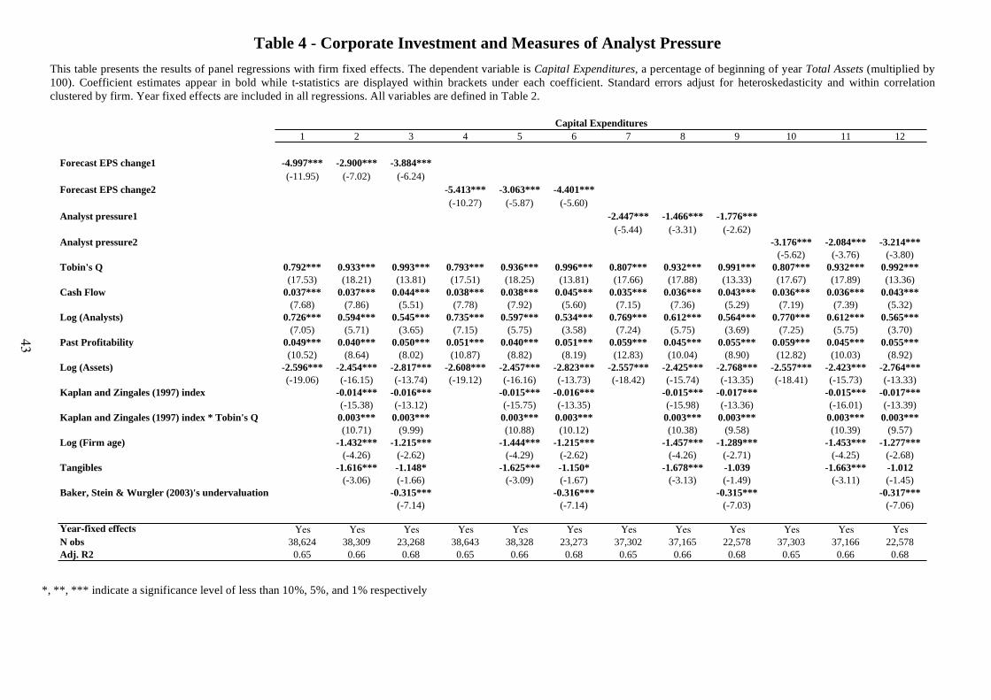
43

Table 4 - Corporate Investment and Measures of Analyst Pressure

This table presents the results of panel regressions with firm fixed effects. The dependent variable is Capital Expenditures, a percentage of beginning of year Total Assets (multiplied by

100). Coefficient estimates appear in bold while t-statistics are displayed within brackets under each coefficient. Standard errors adjust for heteroskedasticity and within correlation

clustered by firm. Year fixed effects are included in all regressions. All variables are defined in Table 2.


1 2 3 4 5 6 7 8 9 10 11 12

Forecast EPS change1 -4.997*** -2.900*** -3.884***

(-11.95) (-7.02) (-6.24)


(-10.27) (-5.87) (-5.60)

Analyst pressure1 -2.447*** -1.466*** -1.776***

(-5.44) (-3.31) (-2.62)


(-5.62) (-3.76) (-3.80)

Tobin's Q 0.792*** 0.933*** 0.993*** 0.793*** 0.936*** 0.996*** 0.807*** 0.932*** 0.991*** 0.807*** 0.932*** 0.992***

(17.53) (18.21) (13.81) (17.51) (18.25) (13.81) (17.66) (17.88) (13.33) (17.67) (17.89) (13.36)

Cash Flow 0.037*** 0.037*** 0.044*** 0.038*** 0.038*** 0.045*** 0.035*** 0.036*** 0.043*** 0.036*** 0.036*** 0.043***

(7.68) (7.86) (5.51) (7.78) (7.92) (5.60) (7.15) (7.36) (5.29) (7.19) (7.39) (5.32)

Log (Analysts) 0.726*** 0.594*** 0.545*** 0.735*** 0.597*** 0.534*** 0.769*** 0.612*** 0.564*** 0.770*** 0.612*** 0.565***

(7.05) (5.71) (3.65) (7.15) (5.75) (3.58) (7.24) (5.75) (3.69) (7.25) (5.75) (3.70)

Past Profitability 0.049*** 0.040*** 0.050*** 0.051*** 0.040*** 0.051*** 0.059*** 0.045*** 0.055*** 0.059*** 0.045*** 0.055***

(10.52) (8.64) (8.02) (10.87) (8.82) (8.19) (12.83) (10.04) (8.90) (12.82) (10.03) (8.92)

Log (Assets) -2.596*** -2.454*** -2.817*** -2.608*** -2.457*** -2.823*** -2.557*** -2.425*** -2.768*** -2.557*** -2.423*** -2.764***

(-19.06) (-16.15) (-13.74) (-19.12) (-16.16) (-13.73) (-18.42) (-15.74) (-13.35) (-18.41) (-15.73) (-13.33)

Kaplan and Zingales (1997) index -0.014*** -0.016*** -0.015*** -0.016*** -0.015*** -0.017*** -0.015*** -0.017***

(-15.38) (-13.12) (-15.75) (-13.35) (-15.98) (-13.36) (-16.01) (-13.39)

Kaplan and Zingales (1997) index * Tobin's Q 0.003*** 0.003*** 0.003*** 0.003*** 0.003*** 0.003*** 0.003*** 0.003***

(10.71) (9.99) (10.88) (10.12) (10.38) (9.58) (10.39) (9.57)

Log (Firm age) -1.432*** -1.215*** -1.444*** -1.215*** -1.457*** -1.289*** -1.453*** -1.277***

(-4.26) (-2.62) (-4.29) (-2.62) (-4.26) (-2.71) (-4.25) (-2.68)

Tangibles -1.616*** -1.148* -1.625*** -1.150* -1.678*** -1.039 -1.663*** -1.012

(-3.06) (-1.66) (-3.09) (-1.67) (-3.13) (-1.49) (-3.11) (-1.45)

Baker, Stein & Wurgler (2003)'s undervaluation -0.315*** -0.316*** -0.315*** -0.317***

(-7.14) (-7.14) (-7.03) (-7.06)

Year-fixed effects Yes Yes Yes Yes Yes Yes Yes Yes Yes Yes Yes YesN obs 38,624 38,309 23,268 38,643 38,328 23,273 37,302 37,165 22,578 37,303 37,166 22,578

Adj. R2 0.65 0.66 0.68 0.65 0.66 0.68 0.65 0.66 0.68 0.65 0.66 0.68

Capital Expenditures

44

Table 5 - Earnings Surprises and Corporate Investment

This table presents the results of panel logit regressions with firm fixed effects. The dependent variable is Non-negative EPS

surprise, a dummy variable equal to 1 when the firm posts earnings per share (EPS) superior to the analysts’ last outstanding

consensus EPS forecast before the fiscal year EPS announcement and equal to 0 otherwise. Coefficient estimates appear in bold

while z-statistics are displayed within brackets under each coefficient. Standard errors adjust for heteroskedasticity and within

correlation clustered by firm. Marginal Effects are presented for model 4: they are computed at the mean values of variables, assuming fixed effects are equal to zero (the logit with fixed effects estimation does not explicitely estimates fixed effects). Year

fixed effects are included in all regressions. All variables are defined in Table 2.

Panel A – Non-negative EPS Surprises and Capital Expenditures


Marginal

Effects

1 2 3 4 model 4 5

Capital expenditures -0.575*** -0.617*** -0.740*** -0.775*** -0.178 -0.894***

(-2.73) (-2.92) (-3.19) (-3.33) (-3.33)

Sales 0.262*** 0.260*** 0.189*** 0.202*** 0.046 0.095**

(6.88) (6.81) (4.49) (4.71) (1.91)

Cash Flow 3.699*** 3.644*** 2.881*** 2.893*** 0.666 1.746***

(19.37) (19.20) (14.16) (14.10) (8.82)

Log (Analysts) 0.057** 0.057** -0.043 -0.040 -0.009 0.025

(2.08) (2.08) (-1.31) (-1.21) (0.62)

Log (Assets) -0.040 -0.043 -0.067* -0.082** -0.015 -0.096**

(-1.16) (-1.26) (-1.76) (-2.08) (-1.98)

Past Profitability -0.727*** -0.706*** -0.848*** -0.895*** -0.206 -0.948***

(-6.14) (-5.96) (-6.58) (-6.85) (6.48)

Changes in total accruals 0.305*** 0.315*** 0.183* 0.186** 0.043 0.052

(3.66) (3.76) (1.96) (1.99) (0.47)

Percentage Non-negative EPS surprise in industry 0.342*** 0.337*** 0.335*** 0.077 0.300***

(5.12) (4.60) (4.56) (3.10)

Standard deviation of forecasts -0.068** -0.065** -0.017 0.003

(-2.05) (-2.00) (0.09)

Positive EPS 0.559*** 0.553*** 0.130 0.958***

(12.00) (11.80) (16.16)

Upwards Consensus Change 0.173*** 0.173*** 0.040 0.442***

(6.18) (6.18) (12.66)

Log(Age) -0.014 -0.003 -0.152

(-0.16) (-1.43)

Tangibles -0.309*** -0.071 -0.250*

(-2.78) (-1.80)

Analyst pressure1 -0.608**

(-2.48)

Year-fixed effects Yes Yes Yes Yes Yes Yes

N obs 43,539 43,030 36,405 36,356 25,425

Pseudo R2 0.05 0.05 0.06 0.06 0.07

Non-negative EPS surprise Non-negative EPS surprise

Dependent Variable: Dependent Variable:

45

Table 5 (continued)

Panel B – Non-negative EPS Surprises and Depreciation Expenses


1 2 3 4

Depreciation -3.480*** -3.392*** -2.693*** -2.236**

(-4.71) (-4.60) (-3.26) (-2.52)

Sales 0.287*** 0.282*** 0.196*** 0.198***

(7.46) (7.33) (4.57) (4.57)

Cash Flow 3.651*** 3.597*** 2.843*** 2.852***

(19.29) (19.14) (14.18) (14.20)

Log (Analysts) 0.056** 0.056** -0.044 -0.044

(2.10) (2.08) (-1.38) (-1.36)

Log (Assets) -0.046 -0.048 -0.067* -0.072*

(-1.35) (-1.41) (-1.79) (-1.85)

Past Profitability -0.794*** -0.776*** -0.910*** -0.940***

(-6.67) (-6.52) (-7.06) (-7.20)

Changes in total accruals 0.320*** 0.330*** 0.204** 0.203**

(3.86) (3.95) (2.19) (2.17)

0.331*** 0.335*** 0.332***

(5.01) (4.61) (4.57)

Standard deviation of forecasts -0.065** -0.064**

(-2.02) (-2.00)

Positive EPS 0.545*** 0.543***

(11.72) (11.65)

Upwards Consensus Change 0.176*** 0.176***

(6.32) (6.34)

Log(Age) -0.017

(-0.18)

Tangibles -0.169

(-1.44)

Year-fixed effects Yes Yes Yes Yes

N obs 44,053 43,543 36,862 36,809

Pseudo R2 0.05 0.05 0.06 0.06

Non-negative EPS surprise

Percentage Non-negative EPS surprise in industry

Dependent Variable:

46

Table 6 – Earnings Surprises, Corporate Investment and Bad News

This table presents the results of panel logit regressions with firm fixed effects where the dependent variable is Non-negative

EPS surprise, a dummy variable equal to 1 when the firm posts earnings per share (EPS) equal to or superior to the analysts’ last

outstanding consensus EPS forecast before the fiscal year EPS announcement and equal to 0 otherwise. Coefficient estimates

appear in bold while z-statistics are displayed within brackets under each coefficient. Standard errors adjust for

heteroskedasticity and within correlation clustered by firm. Year fixed effects are included in all regressions. All variables are defined in Table 2.


1 2 3 4

Capital expenditures -0.681*** -0.728*** -0.719*** -0.778***

(-2.74) (-2.92) (-2.71) (-2.93)

Capital expenditures*Bad News 0.282 0.307 0.279 0.269

(0.73) (0.80) (0.66) (0.63)

Bad news -0.194*** -0.193*** 0.031 0.034

(-4.40) (-4.37) (0.60) (0.65)

Sales 0.211*** 0.208*** 0.083* 0.101**

(4.94) (4.85) (1.85) (2.23)

Cash Flow 3.136*** 3.090*** 1.891*** 1.893***

(16.10) (15.97) (10.06) (10.04)

Log (Analysts) 0.069** 0.070** 0.007 0.015

(2.14) (2.16) (0.18) (0.40)

Log (Assets) -0.059 -0.061 -0.088** -0.092**

(-1.46) (-1.51) (-2.05) (-2.03)


(-5.70) (-5.55) (-5.84) (-6.18)

Changes in total accruals 0.223** 0.233** 0.071 0.075

(2.33) (2.42) (0.67) (0.71)

Percentage above EPS forecasts in industry 0.377*** 0.315*** 0.313***

(4.82) (3.72) (3.69)

Standard deviation of forecasts -0.020 -0.019

(-0.91) (-0.86)

Positive EPS 0.874*** 0.870***

(16.35) (16.22)

Downwards consensus revisions -0.413*** -0.413***

(-12.42) (-12.38)

Log(Age) -0.140

(-1.40)

Tangibles -0.258**

(-1.99)


N obs 33,088 32,701 28,851 28,812

Pseudo R2 0.05 0.05 0.06 0.06


Dependent Variable:

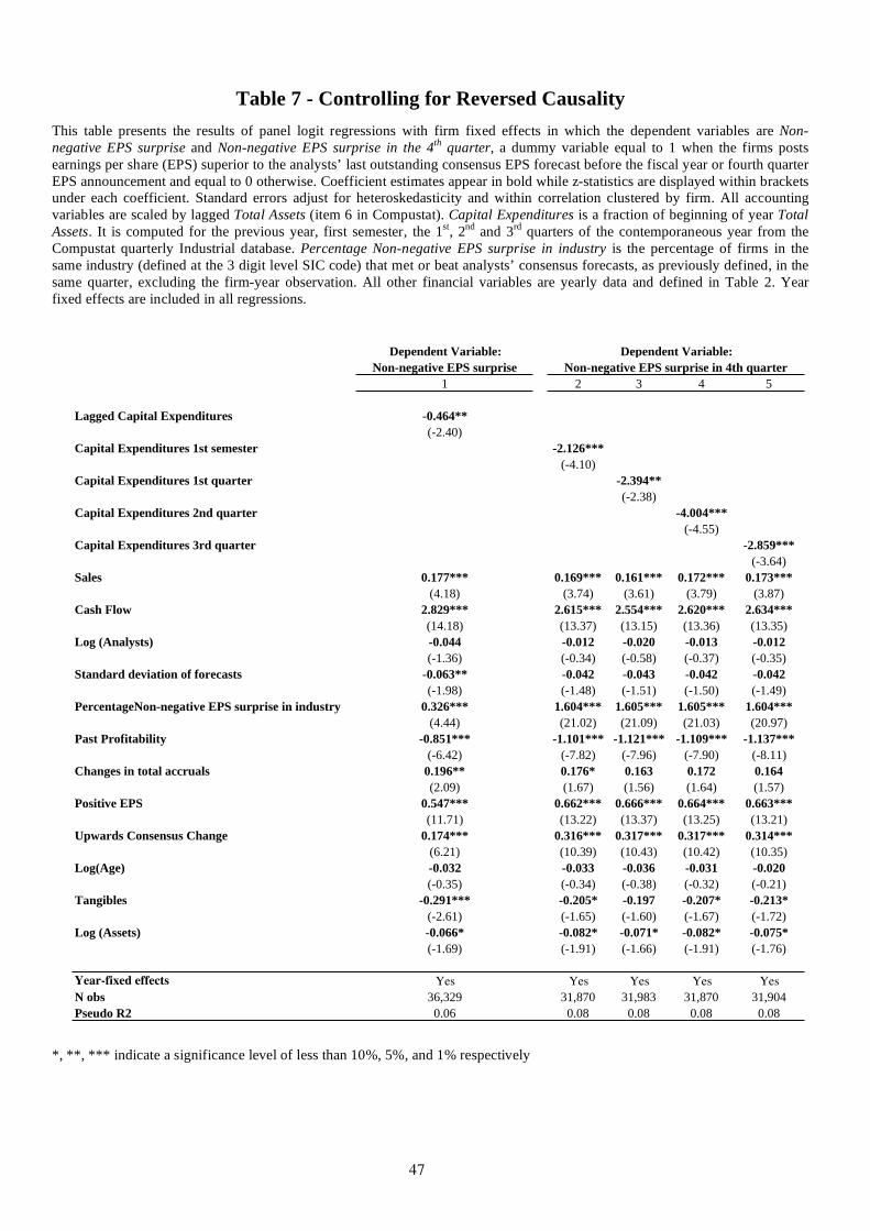
47

Table 7 - Controlling for Reversed Causality

This table presents the results of panel logit regressions with firm fixed effects in which the dependent variables are Non-

negative EPS surprise and Non-negative EPS surprise in the 4th

quarter, a dummy variable equal to 1 when the firms posts

earnings per share (EPS) superior to the analysts’ last outstanding consensus EPS forecast before the fiscal year or fourth quarter

EPS announcement and equal to 0 otherwise. Coefficient estimates appear in bold while z-statistics are displayed within brackets under each coefficient. Standard errors adjust for heteroskedasticity and within correlation clustered by firm. All accounting

variables are scaled by lagged Total Assets (item 6 in Compustat). Capital Expenditures is a fraction of beginning of year Total

Assets. It is computed for the previous year, first semester, the 1st, 2nd and 3rd quarters of the contemporaneous year from the

Compustat quarterly Industrial database. Percentage Non-negative EPS surprise in industry is the percentage of firms in the

same industry (defined at the 3 digit level SIC code) that met or beat analysts’ consensus forecasts, as previously defined, in the

same quarter, excluding the firm-year observation. All other financial variables are yearly data and defined in Table 2. Year

fixed effects are included in all regressions.


Dependent Variable:


1 2 3 4 5

Lagged Capital Expenditures -0.464**

(-2.40)

Capital Expenditures 1st semester -2.126***

(-4.10)

Capital Expenditures 1st quarter -2.394**

(-2.38)

Capital Expenditures 2nd quarter -4.004***

(-4.55)

Capital Expenditures 3rd quarter -2.859***

(-3.64)

Sales 0.177*** 0.169*** 0.161*** 0.172*** 0.173***

(4.18) (3.74) (3.61) (3.79) (3.87)

Cash Flow 2.829*** 2.615*** 2.554*** 2.620*** 2.634***

(14.18) (13.37) (13.15) (13.36) (13.35)

Log (Analysts) -0.044 -0.012 -0.020 -0.013 -0.012

(-1.36) (-0.34) (-0.58) (-0.37) (-0.35)

Standard deviation of forecasts -0.063** -0.042 -0.043 -0.042 -0.042

(-1.98) (-1.48) (-1.51) (-1.50) (-1.49)

PercentageNon-negative EPS surprise in industry 0.326*** 1.604*** 1.605*** 1.605*** 1.604***

(4.44) (21.02) (21.09) (21.03) (20.97)

Past Profitability -0.851*** -1.101*** -1.121*** -1.109*** -1.137***

(-6.42) (-7.82) (-7.96) (-7.90) (-8.11)

Changes in total accruals 0.196** 0.176* 0.163 0.172 0.164

(2.09) (1.67) (1.56) (1.64) (1.57)

Positive EPS 0.547*** 0.662*** 0.666*** 0.664*** 0.663***

(11.71) (13.22) (13.37) (13.25) (13.21)

Upwards Consensus Change 0.174*** 0.316*** 0.317*** 0.317*** 0.314***

(6.21) (10.39) (10.43) (10.42) (10.35)

Log(Age) -0.032 -0.033 -0.036 -0.031 -0.020

(-0.35) (-0.34) (-0.38) (-0.32) (-0.21)

Tangibles -0.291*** -0.205* -0.197 -0.207* -0.213*

(-2.61) (-1.65) (-1.60) (-1.67) (-1.72)

Log (Assets) -0.066* -0.082* -0.071* -0.082* -0.075*

(-1.69) (-1.91) (-1.66) (-1.91) (-1.76)

Year-fixed effects Yes Yes Yes Yes YesN obs 36,329 31,870 31,983 31,870 31,904

Pseudo R2 0.06 0.08 0.08 0.08 0.08

Non-negative EPS surprise in 4th quarter

Dependent Variable:

48

Table 8 - Controlling for Firms’ Investment Opportunities

Panel A presents the results of panel regressions with firm fixed effects. The dependent variable is Capital

Expenditures, a fraction of beginning of year Total Assets multiplied by 100. Coefficient estimates appear in bold while

t-statistics are displayed within brackets under each coefficient. Standard errors adjust for heteroskedasticity and within

correlation clustered by firm. Forecast EPS change1, Forecast EPS change2, Analyst Pressure1 and Analyst Pressure2

are proxies for the level of pressure exerted by analyst at the start of the year on the firm’s management to increase

earnings per share (EPS). These variables are interacted with a dummy variable equal to 1 when the firm’s Tobin’s Q

falls in the highest tercile (High Tobin’s Q) at the beginning of the year. All other variables are defined in Table 2. Year fixed effects are included.

Panel A


1 2 3 4

Forecast EPS change1 -4.938***

(-11.18)

High Tobin's Q * Forecast EPS change1 0.735

(0.69)

Forecast EPS change2 -5.347***

(-9.60)

High Tobin's Q * Forecast EPS change2 0.734

(0.59)

Analyst pressure1 -1.875***

(-3.81)

High Tobin's Q * Analyst pressure1 -2.256*

(-1.82)

Analyst pressure2 -2.283***

(-3.67)

High Tobin's Q * Analyst pressure2 -3.631**

(-2.38)

High Tobin's Q 1.356*** 1.365*** 1.347*** 1.344***

(10.26) (10.19) (10.28) (10.29)

Tobin's Q 0.634*** 0.634*** 0.650*** 0.650***

(13.88) (13.84) (13.97) (14.00)

Cash Flow 0.035*** 0.035*** 0.033*** 0.034***

(7.25) (7.35) (6.78) (6.84)

Log (Analysts) 0.654*** 0.663*** 0.703*** 0.704***

(6.37) (6.47) (6.64) (6.66)

Log (Assets) -2.507*** -2.519*** -2.470*** -2.469***

(-18.59) (-18.65) (-17.98) (-17.98)

Past Profitability 0.044*** 0.045*** 0.054*** 0.054***

(9.40) (9.74) (11.87) (11.87)


N obs 38,624 38,643 37,302 37,303

Adj. R2 0.66 0.66 0.66 0.66


Dependent Variable:

49

Table 8 (continued)

Panel B presents the results of panel logit regressions run separately for three portfolios of firm-year observations that

are based on the tercile in which a firm’s start-of-the-year Tobin’s Q falls for each year. The regression is run with firm

fixed effects. The dependent variable is Non-negative EPS surprise, a dummy variable equal to 1 when the firms posts

earnings per share (EPS) superior to the analysts’ last outstanding consensus EPS forecast before the fiscal year EPS

announcement and equal to 0 otherwise. Coefficient estimates appear in bold while z-statistics are displayed within

brackets under each coefficient. Standard errors adjust for heteroskedasticity and within correlation clustered by firm.

Year fixed effects are included in all regressions. All variables are defined in Table 2.

Panel B


Low Tobin's Q High Tobin's Q

T1 T2 T3

Capital Expenditures -0.687 -1.302** -1.762***

(-1.27) (-2.45) (-3.92)

Sales -0.021 0.088 0.160*

(-0.20) (1.01) (1.85)

Cash Flow 2.813*** 2.743*** 1.328***

(4.27) (5.21) (5.56)

Log (Analysts) -0.084 0.036 -0.083

(-1.15) (0.52) (-1.11)

Percentage Non-negative EPS surprise in industry 0.445*** 0.213 0.341*

(3.08) (1.43) (1.83)

Changes in total accruals 0.272 0.124 0.055

(1.22) (0.57) (0.32)

Upwards Consensus change 0.371*** 0.454*** 0.474***

(5.65) (7.83) (7.86)

Positive EPS 1.535*** 1.216*** 1.043***

(14.00) (9.06) (7.90)

Past Profitability -1.933*** -0.761** -0.635***

(-3.99) (-2.12) (-3.26)

Log (Assets) 0.016 -0.218*** -0.097

(0.16) (-2.63) (-1.20)

Year-fixed effects Yes Yes Yes

N obs 7,617 8,654 8,303

Pseudo R2 0.10 0.07 0.06


Dependent Variable:

50

Table 9 – Investment Manipulation: a Last Resort?

Panel A presents the results of panel regression with firm fixed effects. The dependent variable is Capital Expenditures, a

fraction of beginning of year Total Assets multiplied by 100. Coefficient estimates appear in bold while t-statistics are displayed within brackets under each coefficient. Standard errors adjust for heteroskedasticity and within correlation

clustered by firm. Analyst Pressure1 is a proxy for the level of pressure exerted by analyst at the start of the year on the

firm’s management to increase earnings per share (EPS). This variable is interacted with a dummy variable, High past

accruals, equal to 1 if the previous year Total Accruals scaled by lagged Total Assets is in the top quartile of lagged Total

Accruals (High Past Accruals) at the beginning of the year, and equal to 0 otherwise. Year fixed effects are included. All

other variables are defined in Table 2.

Panel A


1 2 3 4

Analyst pressure1 -2.393*** -1.622*** -1.368*** -1.833**

(-4.85) (-3.35) (-2.84) (-2.56)

Analyst pressure1 * High past accruals -0.356 -0.607 -0.607 0.297

(-0.26) (-0.46) (-0.46) (0.14)

High past accruals -0.102 -0.103 -0.182** -0.123

(-1.20) (-1.22) (-2.12) (-1.08)

Tobin's Q 0.810*** 0.952*** 0.936*** 0.993***

(17.67) (18.04) (17.88) (13.32)

Cash Flow 0.035*** 0.035*** 0.036*** 0.043***

(7.13) (7.15) (7.34) (5.28)

Log (Analysts) 0.768*** 0.561*** 0.611*** 0.565***

(7.24) (5.31) (5.74) (3.70)

Past Profitability 0.060*** 0.048*** 0.046*** 0.056***

(12.56) (10.32) (10.03) (8.80)

Log (Assets) -2.557*** -2.364*** -2.425*** -2.769***

(-18.40) (-17.33) (-15.73) (-13.35)

Kaplan and Zingales (1997) index -0.015*** -0.015*** -0.017***

(-15.98) (-15.98) (-13.36)

Kaplan and Zingales (1997) index * Tobin's Q 0.003*** 0.003*** 0.003***

(10.18) (10.36) (9.58)

Log (Firm age) -1.483*** -1.307***

(-4.31) (-2.73)

Tangible Assets -1.717*** -1.070

(-3.20) (-1.53)

Baker, Stein & Wurgler (2003)'s undervaluation -0.315***

(-7.02)


N obs 37,302 37,302 37,165 22,578

Pseudo R2 0.65 0.66 0.66 0.68


Dependent Variable:

51

Table 9 (continued)

Panel B

Panel B presents the results of panel logit regressions with firm fixed effects. The dependent variable is Non-negative EPS

surprise, a dummy variable equal to 1 when the firm posts earnings per share (EPS) equal to or superior to the analysts’ last

outstanding consensus EPS forecast before the fiscal year EPS announcement, and equal to 0 otherwise. Coefficient estimates

appear in bold while z-statistics are displayed within brackets under each coefficient. Standard errors adjust for

heteroskedasticity and within correlation clustered by firm. Capital Expenditures is a fraction of beginning of year Total

Assets. High past accruals is a dummy variable equal to 1 if the previous year Total Accruals scaled by lagged Total Assets is

in the top quartile of lagged Total Accruals, and equal to 0 otherwise. Capital Expenditures * High past accruals is the

interaction term between these two variables. Year fixed effects are included in all regressions. All other variables are defined in Table 2.


1 2 3 4

Capital expenditures -0.492** -0.535** -0.850*** -0.877***

(-2.16) (-2.35) (-3.17) (-3.25)

Capital expenditures * High past accruals -0.003 -0.003 -0.003 -0.003

(-1.01) (-1.00) (-0.82) (-0.87)

High past accruals 0.019 0.019 -0.042 -0.048

(0.46) (0.45) (-0.84) (-0.97)

Sales 0.263*** 0.261*** 0.083* 0.096**

(6.90) (6.84) (1.94) (2.19)

Cash Flow 3.701*** 3.646*** 1.689*** 1.691***

(19.33) (19.16) (9.40) (9.39)

Log (Analysts) 0.057** 0.057** -0.006 -0.002

(2.07) (2.06) (-0.16) (-0.05)

Log (Assets) -0.041 -0.044 -0.075* -0.067

(-1.18) (-1.28) (-1.88) (-1.59)


(-6.07) (-5.89) (-6.30) (-6.51)

Changes in total accruals 0.298*** 0.308*** 0.016 0.005

(3.05) (3.13) (0.14) (0.05)

Percentage above EPS forecasts in industry 0.341*** 0.340*** 0.337***

(5.11) (4.28) (4.24)

Standard deviation of forecasts 0.010 0.010

(0.36) (0.37)

Positive EPS 0.997*** 0.995***

(19.34) (19.24)

Downwards consensus revisions -0.410*** -0.409***

(-13.49) (-13.44)

Log(Age) -0.144

(-1.50)

Tangibles -0.093

(-0.77)


N obs 43,539 43,030 31,542 31,497

Pseudo R2 0.05 0.05 0.07 0.07


Dependent Variable:

52

Table 10 - Robustness Checks:

Alternative Measure of Analyst Consensus Forecasts

This table presents the results of panel logit regressions with firm fixed effects. The dependent variable is Actual EPS above

last EPS forecast, a dummy variable equal to 1 when the firms posts earnings per share (EPS) superior to the last analyst EPS forecast before the fiscal year EPS announcement, and equal to 0 otherwise. Coefficient estimates appear in bold while

z-statistics are displayed within brackets under each coefficient. Standard errors adjust for heteroskedasticity and within

correlation clustered by firm. Year fixed effects are included in all regressions. All other variables are defined in Table 2.


1 2 3 4

Capital Expenditures -0.519* -0.500* -0.772*** -0.721**

(-1.93) (-1.86) (-2.65) (-2.48)

Sales 0.250*** 0.240*** 0.039 0.030

(5.02) (4.83) (0.74) (0.56)

Cash Flow 2.740*** 2.711*** 0.830*** 0.855***

(13.73) (13.61) (4.17) (4.28)

Log (Analysts) -0.002 -0.006 -0.055 -0.060

(-0.06) (-0.15) (-1.30) (-1.41)

Log (Assets) -0.220*** -0.224*** -0.276*** -0.371***

(-4.85) (-4.88) (-5.54) (-7.02)

Past Profitability -0.104 -0.091 -0.527*** -0.498***

(-0.69) (-0.61) (-3.28) (-3.06)

Changes in total accruals 0.390*** 0.385*** 0.180 0.169

(3.86) (3.78) (1.60) (1.50)

Percentage above last EPS forecasts in industry 0.246*** 0.292*** 0.279***

(2.71) (2.95) (2.81)


(0.21) (0.33)

Positive EPS 1.608*** 1.604***

(22.56) (22.60)


(10.40) (10.52)

Log(Age) 0.705***

(5.82)

Tangibles -0.509***

(-3.39)


N obs 32,297 31,731 27,524 27,476

Pseudo R2 0.04 0.04 0.08 0.08

Actual EPS above last EPS forecast

Dependent Variable:

53


Sales Surprises and Corporate Investment

This table presents the results of panel logit regressions with firm fixed effects. The dependent variable is Non-negative

Sales surprise, a dummy variable equal to 1 when the firms posts sales superior to the last analysts consensus sales forecast

before the fiscal year sales announcement, and equal to 0 otherwise. Coefficient estimates appear in bold while z-statistics are displayed within brackets under each coefficient. Standard errors adjust for heteroskedasticity and within correlation

clustered by firm. Percentage Non-negative Sales surprise in industry is the percentage of firms in the same industry

(defined at the 3 digit level SIC code) that met or beat analysts’ sales consensus forecasts, as previously defined, in the

same fiscal year, excluding the firm-year observation. Year fixed effects are included in all regressions. All other variables

are defined in Table 2.


1 2 3 4

Capital Expenditures -0.003 -0.003 -0.003 -0.006

(-0.64) (-0.51) (-0.60) (-1.08)

Sales 0.606*** 0.595*** 0.480*** 0.508***

(7.19) (7.03) (5.44) (5.65)

Cash Flow 0.690*** 0.634*** 0.358 0.392*

(3.18) (2.93) (1.55) (1.69)

Log (Analysts) -0.015 -0.025 -0.067 -0.066

(-0.28) (-0.45) (-1.11) (-1.09)

Log (Assets) -0.120 -0.114 -0.147* -0.225***

(-1.62) (-1.51) (-1.85) (-2.59)


(-4.88) (-4.56) (-4.29) (-4.36)

Changes in total accruals -0.106 -0.134 -0.236 -0.231

(-0.66) (-0.82) (-1.36) (-1.33)

Percentage Non-negative sales surprise in industry 0.863*** 0.835*** 0.829***

(7.04) (6.55) (6.47)


(0.17) (0.23)

Positive EPS 0.298*** 0.287***

(3.66) (3.53)


(6.30) (6.19)

Log(Age) -0.356

(-1.42)

Tangibles -0.748***

(-2.82)


N obs 11,793 11,507 10,588 10,562

Pseudo R2 0.04 0.05 0.05 0.05

Non-negative Sales surprise

Dependent Variable:

54


Corporate Investment and Analyst Pressure, Excluding Large Past Investment Firm-Year Observations

This table presents the results of panel regressions with firm fixed effects. The dependent variable is Capital Expenditures, a fraction of beginning of year Total Assets (item 6) multiplied by

100. Coefficient estimates appear in bold while t-statistics are displayed within brackets under each coefficient. Standard errors adjust for heteroskedasticity and within correlation clustered

by firm. The sample excludes firms that had lagged capital expenditures in the top quintile. Year fixed effects are included in all regressions. All other variables are defined in Table 2.


1 2 3 4 5 6 7 8 9 10 11 12


(-10.88) (-8.35) (-8.97)


(-7.59) (-3.98) (-4.34)


(-8.67) (-7.78) (-5.08)


(-7.67) (-7.06) (-5.15)

Tobin's Q 0.278*** 0.319*** 0.357*** 0.831*** 1.024*** 1.009*** 0.295*** 0.330*** 0.362*** 0.295*** 0.330*** 0.363***

(16.47) (16.07) (12.91) (15.43) (16.89) (12.20) (17.41) (16.59) (12.65) (17.41) (16.60) (12.68)

Cash Flow 0.018*** 0.017*** 0.024*** 0.041*** 0.042*** 0.046*** 0.017*** 0.017*** 0.022*** 0.017*** 0.017*** 0.022***

(11.98) (11.79) (9.35) (6.34) (6.57) (4.62) (11.36) (11.26) (8.77) (11.34) (11.26) (8.74)

Log (Analysts) 0.298*** 0.234*** 0.216*** 0.747*** 0.570*** 0.466*** 0.297*** 0.231*** 0.221*** 0.298*** 0.231*** 0.221***

(7.32) (5.74) (3.52) (6.07) (4.59) (2.72) (7.05) (5.52) (3.52) (7.07) (5.53) (3.53)

Past Profitability 0.022*** 0.019*** 0.020*** 0.057*** 0.045*** 0.059*** 0.026*** 0.021*** 0.024*** 0.026*** 0.021*** 0.024***

(13.26) (11.64) (8.06) (9.09) (7.38) (7.33) (16.00) (13.40) (9.42) (16.03) (13.43) (9.49)

Log (Assets) -0.661*** -0.496*** -0.639*** -3.033*** -2.794*** -3.228*** -0.620*** -0.464*** -0.625*** -0.620*** -0.463*** -0.624***

(-12.83) (-8.71) (-8.29) (-19.19) (-15.62) (-13.72) (-11.83) (-8.05) (-7.90) (-11.83) (-8.03) (-7.88)

Kaplan and Zingales (1997) index -0.005*** -0.006*** -0.016*** -0.016*** -0.006*** -0.007*** -0.006*** -0.007***

(-14.07) (-11.48) (-14.25) (-11.40) (-15.22) (-12.22) (-15.31) (-12.27)

Kaplan and Zingales (1997) index * Tobin's Q 0.001*** 0.001*** 0.003*** 0.003*** 0.001*** 0.001*** 0.001*** 0.001***

(8.38) (6.95) (11.79) (9.14) (8.26) (7.02) (8.32) (7.04)

Log (Firm age) -0.287** -0.112 -1.536*** -1.014* -0.321** -0.158 -0.323** -0.154

(-2.20) (-0.59) (-3.85) (-1.90) (-2.41) (-0.81) (-2.43) (-0.79)

Tangibles 1.028*** 1.244*** -1.745*** -1.464* 0.988*** 1.179*** 0.996*** 1.187***

(5.20) (4.60) (-2.91) (-1.95) (4.89) (4.24) (4.92) (4.27)

Baker, Stein & Wurgler (2003)'s undervaluation -0.110*** -0.377*** -0.112*** -0.113***

(-5.66) (-7.20) (-5.67) (-5.71)

Year-fixed effects Yes Yes Yes Yes Yes Yes Yes Yes Yes Yes Yes YesN obs 30,992 30,729 18,357 31,298 31,133 19,709 29,915 29,794 17,804 29,916 29,795 17,804

Adj. R2 0.64 0.65 0.64 0.65 0.65 0.67 0.64 0.64 0.64 0.64 0.64 0.64


55

Table 13 - Corporate Investment and Cost Structure

All data are collected from the Compustat Quarterly Industrial database for quarterly data and the Compustat Annual Industrial

database for yearly data. Our sample of firms excludes firms not covered by analysts, financial services firms (SIC code 6000-

6999), regulated utilities (SIC code 4900), and firms with book value of equity smaller than $10 million. Panel A presents panel

regressions with firm fixed effects. Year fixed effects are also included in all regressions. All variables are scaled by lagged Total

Assets (item 6 in Compustat). The dependent variables, Depreciation expenses is item 14, and Net Income is net income before

extraordinary items (item 18). Capital Expenditures is item 128. Sales is net sales (item 12), SG&A is Selling, General and

Administrative Expenses (item 189), Cost of Goods Sold is item 41, Tangibles is Gross Property, Plant Equipment (item 7) and Inverse of Total Assets is one divided by lagged total assets (item 6). means that I use the first difference for the variable under

consideration in the regression. Coefficient estimates appear in bold while t-statistics are displayed within brackets under each

coefficient. Standard errors adjust for heteroskedasticity and within correlation clustered by firm. Panel B presents correlation

coefficients between selected variables that are all scaled by lagged total assets (item 6). Rental expenses is item 47 in the

Compustat Industrial Annual database, Advertising expenses is item 45, Labor expenses is item 42. Panel C presents panel

regressions with quarter-year and firm fixed effects where the dependent variable, Quarterly SG&A, is quarterly selling, general

and administrative expenses (item 1 in the Compustat Industrial Quarterly database) scaled by beginning of quarter total assets

(item 44). Coefficient estimates appear in bold while t-statistics are displayed within brackets under each coefficient. Standard

errors adjust for heteroskedasticity and within correlation clustered by firm. All variables are scaled by beginning of quarter Total

Assets (item 44). Quarterly Depreciation is depreciation and amortization (item 5), Lagged Quarterly Capital Expenditures is

lagged capital expenditures for the quarter only, recalculated from Compustat item 90 (cumulated capital expenditures from the beginning of the year to the end of the quarter), and Inverse of Total Assets is one divided by quarterly beginning of quarter total

assets (item 44).

Panel A – Yearly Corporate Investment, Depreciation Expenses, and Net Income


Depreciation Net income

Capital expenditures 0.066***

(25.42)

Sales 0.332***

(25.94)

Depreciation -1.070***

(-19.67)

SG&A -0.296***

(-17.79)

Cost of Goods Sold -0.302

(-19.96)

Tangibles 1.235*** 5.474***

(12.40) (14.39)

Inverse of Total Assets 9.880*** 20.473***

(7.33) (3.81)

Year-fixed effects Yes YesN obs 53,691 49,202

Adj. R2 0.21 0,38

Dependent Variable:

56

Panel B – Correlation Between Yearly Investment, Depreciation,

Rental, Advertising and Labor expenses.

Capital

expenditures

Lagged

Capital expenditures

SG&A

expenses

Depreciation

expenses

Rental

expenses

Advertising

expenses

Labor

expenses

Capital expenditures 1.00

Lagged Capital

expenditures 0.68*** 1.00

SG&A expenses -0.02*** -0.10*** 1.00

Depreciation

expenses 0.47*** 0.43*** 0.06*** 1.00

Rental expenses 0.17*** 0.13*** 0.38*** 0.19*** 1.00

Advertising expenses 0.06*** 0.00 0.45*** 0.01** 0.15*** 1.00

Labor expenses 0.06*** 0.02 0.21*** 0.08*** 0.21** 0.04*

Number of total

observations 64,362 54,373 58,933 64,838 57,678 22,844 5,753


Panel C – Quarterly Corporate Investment and SG&A expenses


Dependent Variable:

Quarterly SG&A

Quarterly depreciation 1.33***

(24.24)

Lagged quarterly capital expenditures 0.07***

(8.77)

Inverse of total assets 0.30***

(6.83)

Quarter-year fixed effects YesN obs 165,746

Adj. R2 0.86

57

Figure 1

Meeting or Beating vs. Missing Analysts’ EPS Consensus Forecasts:

Investment Policy Evolution and Ex-Ante Investment Opportunities Panel A displays the percentage difference in median Capital Expenditures, relative to the full sample, for the sub-sample of firms that met or beat analysts consensus forecast at time t and

the sub-sample of firms that missed. Panel B displays the median firms’ ex-ante investment opportunities (Tobin’s Q) evolution over time for the same two sub-samples. Tobin’s Q is the

lagged market-to-book ratio computed as the market value of equity plus book value of assets minus the book value of equity minus balance sheet deferred taxes scaled by the value of

book assets, all values being measured at the beginning of the fiscal year. Capital Expenditures is (Compustat) item 128 scaled by start-of-year Total Assets.

Panel A – Median Capital Expenditures Panel B – Median Lagged Tobin’s Q

58

Figure 2

Meeting or Beating vs. Missing Analysts’ EPS Consensus Forecasts:

Quarterly Median Capital Expenditures This graph displays the median firms’ Quarterly Capital Expenditures for the sub-sample of firms that met or beat analysts’

consensus forecast at time t and the sub-sample of firms that missed. Quarterly Capital Expenditures is computed from the

cumulated capital expenditures in the Compustat Quarterly Industrial database (item 90) scaled by start-of-year Total Assets

(item 6).

corporate investment and analyst pressure

Documents