correcting for static shift of magnetotelluric data with
TRANSCRIPT

Supplement of Solid Earth, 8, 637–660, 2017http://www.solid-earth.net/8/637/2017/doi:10.5194/se-8-637-2017-supplement© Author(s) 2017. CC Attribution 3.0 License.
Supplement of
Correcting for static shift of magnetotelluric data with airborneelectromagnetic measurements: a case study from Rathlin Basin,Northern IrelandRobert Delhaye et al.
Correspondence to: Robert Delhaye ([email protected])
The copyright of individual parts of the supplement might differ from the CC-BY 3.0 licence.

S1 Comparison with Inversion of Non-rotatedData and Mesh
In order to establish if the choice of mesh and data rotation significantly influ-ences the resulting models, a further comparative inversion was performed usingnon-rotated data and mesh. The non-rotated mesh comprised 64× 80× 82 cellsin size (X,Y,Z), with cells in the central portion of the model of lateral extent400 m by 400 m. The layer thicknesses, initial halfspace resistivity of 30 Ωm,bathymetry and smoothing factors were kept identical to the rotated mesh usedwithin the article. Similarly, the same selection of data and error floors as usedfor the rotated data were applied to the non-rotated data. The resulting mod-els, Nc (i.e., inverted from static shift-corrected, non-rotated data) and No (i.e.,inverted from original, non-rotated data), had normalised RMS misfits of 2.14(63 iterations) and 2.17 (60 iterations) respectively.
Figures S1, S3, S5 and S7 present the diagnostic images of resistivity, ∆ (thelogarithmic resistivity difference), and the normalised cross-gradient value forthe two models Mc and Mo determined for rotated data and meshes. In contrast,S2, S4, S6 and S8 present the same diagnostic images for the comparative modelsNc and No determined for non-rotated data and meshes. By examining theresistivity plots of Nc in comparison to the resistivity plots of Mc, it is clearthat the non-rotated N models recover generally similar structures to theirrotated M counterparts, with an extensive central conductor in Nc of similarextent to the central conductor in Mc associated with the Permian and Triassicsediments. Similarly, both M and N models feature a large resistor in thesouth-east associated with the Dalradian metasedimentary block. Although itis apparent that the non-rotated models have resolved slightly less structure atdepth than the rotated models, the discussion presented here is not intendedto be a comprehensive overview of the topic of model and data rotation. Fordetailed investigation of the effects of rotation on MT inversion, the reader isreferred to other works such as Tietze and Ritter (2013).
As the mesh and data rotation does affect 3D inversion results, it is thechanges in ∆, the logarithmic difference between Nc and No, that are of mostinterest to this research. The small variations between the resistivity images ofNc and Mc have the consequence that the distributions of ∆ are not expectedto be identical, as can be clearly seen. The rotated models M show elevatedvalues of ∆, extending to greater depths than in the non-rotated models N .With the caveat that the resistivity distributions cannot be declared equivalentbetween the M and N models (i.e., the differences observed between N andM models cannot be categorically defined as purely due to rotation), it appearsthat rotation of the inversion mesh and data exaggerate the effects of static shiftcorrection on the resulting model. For example, if the depth slices from 1550 mare considered, the distributions of ∆ for the rotated models M generally showmagnitudes that are elevated approximately a quarter of an order of magnitudegreater than those of the non-rotated models N . It should be noted that evenwith the reduced magnitudes of ∆ in the non-rotated N models, the effects of
1

static shift correction still propagate to 2 km depth within the models.
References
Tietze, K. and Ritter, O.: Three-dimensional magnetotelluric inversion inpractice the electrical conductivity structure of the San Andreas Faultin Central California, Geophysical Journal International, 195, 130, doi:10.1093/gji/ggt234, 2013.
2
55˚06'
55˚09'
55˚12'
55˚15'
850 m
(a)
10
10
10
10
10
10
10
10
55˚06'
55˚09'
55˚12'
55˚15'
(b)
10
10
10
1010
10
10
10
−6˚30' −6˚24' −6˚18' −6˚12'55˚06'
55˚09'
55˚12'
55˚15'
(c)
1550 m
(d)
10
101
0
(e)
10
101
0
−6˚30' −6˚24' −6˚18' −6˚12'
(f)
1
10
100
1000
Resistivity (Ωm)
2100 m
(g)
10
10
10
10
−0.5
0.0
0.5
log10(Mc/Mo)
(h)
10
10
10
10
−6˚30' −6˚24' −6˚18' −6˚12'
0.00
0.25
0.50
0.75
1.00
Magnitude
(i)
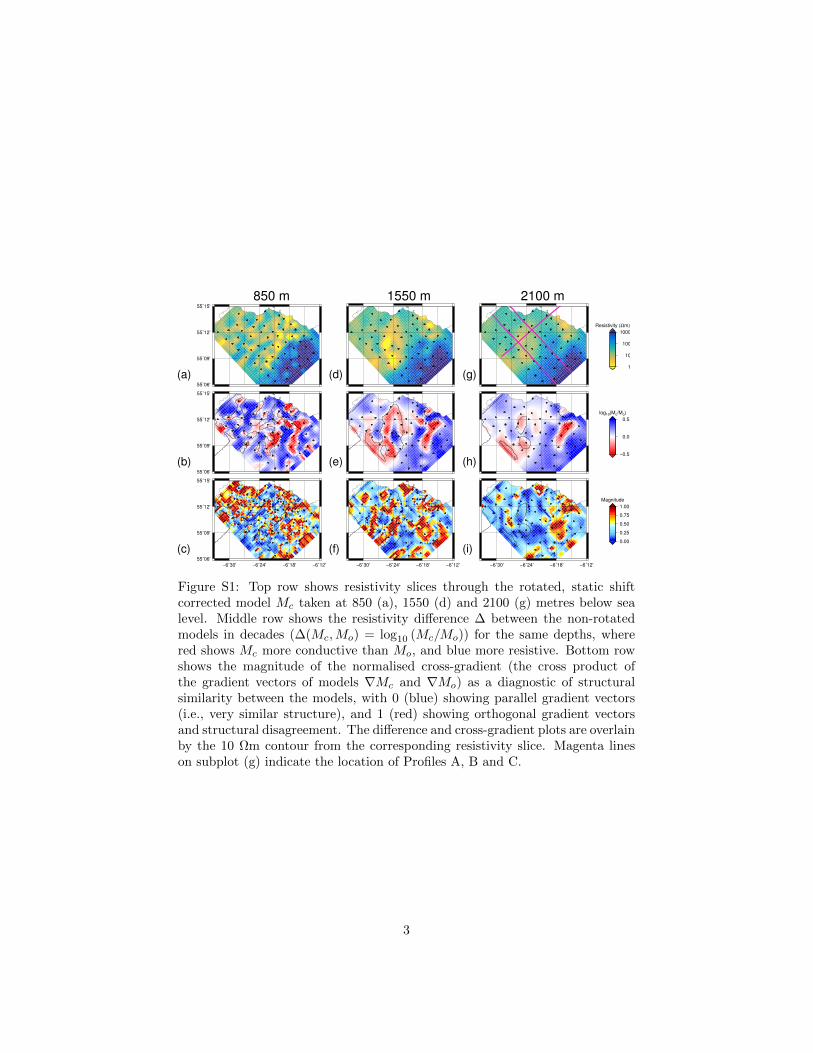
Figure S1: Top row shows resistivity slices through the rotated, static shiftcorrected model Mc taken at 850 (a), 1550 (d) and 2100 (g) metres below sealevel. Middle row shows the resistivity difference ∆ between the non-rotatedmodels in decades (∆(Mc,Mo) = log10 (Mc/Mo)) for the same depths, wherered shows Mc more conductive than Mo, and blue more resistive. Bottom rowshows the magnitude of the normalised cross-gradient (the cross product ofthe gradient vectors of models ∇Mc and ∇Mo) as a diagnostic of structuralsimilarity between the models, with 0 (blue) showing parallel gradient vectors(i.e., very similar structure), and 1 (red) showing orthogonal gradient vectorsand structural disagreement. The difference and cross-gradient plots are overlainby the 10 Ωm contour from the corresponding resistivity slice. Magenta lineson subplot (g) indicate the location of Profiles A, B and C.
3

55˚06'
55˚09'
55˚12'
55˚15'
850 m
(a)
1550 m
(d)1
10
100
1000
Resistivity (Ωm)
2100 m
(g)
(b)55˚06'
55˚09'
55˚12'
55˚15'
(e)−0.5
0.0
0.5
log10(Nc/No)
(h)
−6˚30' −6˚24' −6˚18' −6˚12'55˚06'
55˚09'
55˚12'
55˚15'
(c)
−6˚30' −6˚24' −6˚18' −6˚12'
(f)
−6˚30' −6˚24' −6˚18' −6˚12'
0.00
0.25
0.50
0.75
1.00
Magnitude
(i)
Figure S2: Top row shows resistivity slices through the non-rotated, static shiftcorrected model Nc taken at 850 (a), 1550 (d) and 2100 (g) metres below sealevel. Middle row shows the resistivity difference ∆ between the non-rotatedmodels in decades (∆(Nc, No) = log10 (Nc/No)) for the same depths, wherered shows Nc more conductive than No, and blue more resistive. Bottom rowshows the magnitude of the normalised cross-gradient (the cross product ofthe gradient vectors of models ∇Nc and ∇No) as a diagnostic of structuralsimilarity between the models, with 0 (blue) showing parallel gradient vectors(i.e., very similar structure), and 1 (red) showing orthogonal gradient vectorsand structural disagreement. The difference and cross-gradient plots are overlainby the 10 Ωm contour from the corresponding resistivity slice. Magenta lineson subplot (g) indicate the location of Profiles A, B and C.
4

−3000
−2000
−1000
0
1
10
100
1000
Resistivity (Ωm)
SW NEProfile A
(a)
Depth
(m
b.s
.l.)
−3000
−2000
−1000
0
1010 10
10
−0.50−0.25
0.000.250.50
log10(Mc/Mo)
(b)
Depth
(m
b.s
.l.)
−3000
−2000
−1000
0
0 5000 10000 15000
1010 10
10
0.000.250.500.751.00
Magnitude
(c)
Depth
(m
b.s
.l.)
Distance (m)
Figure S3: Profile A taken along the axis of the concealed basin through thestatic shift corrected resistivity model Mc (location shown on Figures S1g andS2g). The resistivity is shown in (a), the resistivity difference ∆(Mc,Mo) isshown in (b), and the cross-gradient of Mc and Mo is shown in (c). Contours onthe difference and cross-gradient plots show the 10 Ωm contour. For presentationa vertical exaggeration of 1.5 is used.
5

−3000
−2000
−1000
0
1
10
100
1000
Resistivity (Ωm)
SW NEProfile A
(a)
De
pth
(m
b.s
.l.)
−3000
−2000
−1000
0
−0.50−0.25
0.000.250.50
log10(Nc/No)
De
pth
(m
b.s
.l.)
(b)
−3000
−2000
−1000
0
0 5000 10000 15000
0.000.250.500.751.00
Magnitude
(c)
De
pth
(m
b.s
.l.)
Figure S4: Profile A taken along the axis of the concealed basin through the non-rotated, static shift corrected resistivity model Nc (location shown on FiguresS1g and S2g). The resistivity is shown in (a), the resistivity difference ∆(Nc, No)is shown in (b), and the cross-gradient of Nc and No is shown in (c). Contours onthe difference and cross-gradient plots show the 10 Ωm contour. For presentationa vertical exaggeration of 1.5 is used.
6

−3000
−2000
−1000
0
1
10
100
1000
Resistivity (Ωm)
SENW Profile B
(a)
De
pth
(m
b.s
.l.)
−3000
−2000
−1000
0
1010
−0.50−0.25
0.000.250.50
log10(Mc/Mo)
(b)
De
pth
(m
b.s
.l.)
−3000
−2000
−1000
0
05000100001500020000
1010
0.000.250.500.751.00
Magnitude
(c)
De
pth
(m
b.s
.l.)
Distance (m)
Figure S5: Profile B taken across the static shift corrected resistivity modelMc (location shown on Figures S1g and S2g). The resistivity is shown in (a),the resistivity difference ∆(Mc,Mo) is shown in (b), and the cross-gradient ofMc and Mo is shown in (c). Contours on the difference and cross-gradient plotsshow the 10 Ωm contour. For presentation a vertical exaggeration of 1.5 is used.
7
−3000
−2000
−1000
0
1
10
100
1000
Resistivity (Ωm)
−3000
−2000
−1000
0
NW SEProfile B
(a)
Depth
(m
b.s
.l.)
−3000
−2000
−1000
0
−3000
−2000
−1000
0
−0.50
−0.25
0.00
0.25
0.50
log10(Nc/No)
(b)
Depth
(m
b.s
.l.)
−3000
−2000
−1000
0
05000100001500020000
0.00
0.25
0.50
0.75
1.00
Magnitude
−3000
−2000
−1000
0
05000100001500020000
(c)
Depth
(m
b.s
.l.)
Distance (m)
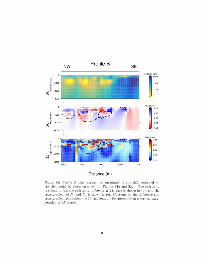
Figure S6: Profile B taken across the non-rotated, static shift corrected re-sistivity model Nc (location shown on Figures S1g and S2g). The resistivityis shown in (a), the resistivity difference ∆(Mc,Mo) is shown in (b), and thecross-gradient of Nc and No is shown in (c). Contours on the difference andcross-gradient plots show the 10 Ωm contour. For presentation a vertical exag-geration of 1.5 is used.
8

−3000
−2000
−1000
0
1
10
100
1000
Resistivity (Ωm)
SENW Profile C
(a)
De
pth
(m
b.s
.l.)
−3000
−2000
−1000
010
10
−0.50−0.25
0.000.250.50
log10(Mc/Mo)
(b)
De
pth
(m
b.s
.l.)
−3000
−2000
−1000
0
05000100001500020000
10
10
0.000.250.500.751.00
Magnitude
(c)
De
pth
(m
b.s
.l.)
Distance (m)
Figure S7: Profile C taken across the static shift corrected resistivity modelMc (location shown on Figures S1g and S2g). The resistivity is shown in (a),the resistivity difference ∆(Mc,Mo) is shown in (b), and the cross-gradient ofMc and Mo is shown in (c). Contours on the difference and cross-gradient plotsshow the 10 Ωm contour. For presentation a vertical exaggeration of 1.5 is used.
9
−3000
−2000
−1000
0
1
10
100
1000
Resistivity (Ωm)
−3000
−2000
−1000
0
NW SEProfile C
(a)
Depth
(m
b.s
.l.)
−3000
−2000
−1000
0
−0.50−0.25
0.000.250.50
log10(Nc/No)
−3000
−2000
−1000
0
(b)
Depth
(m
b.s
.l.)
0.00
0.25
0.50
0.75
1.00
Magnitude
−3000
−2000
−1000
0
050001000015000
(c)
Depth
(m
b.s
.l.)
Distance (m)
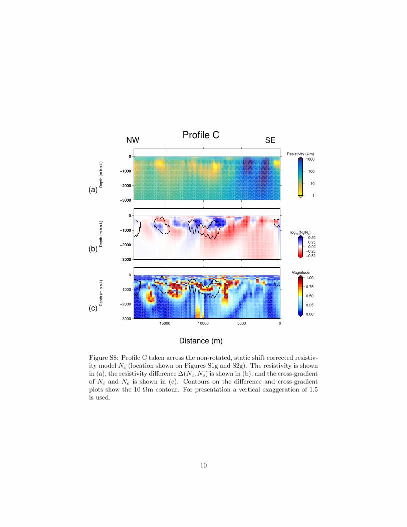
Figure S8: Profile C taken across the non-rotated, static shift corrected resistiv-ity model Nc (location shown on Figures S1g and S2g). The resistivity is shownin (a), the resistivity difference ∆(Nc, No) is shown in (b), and the cross-gradientof Nc and No is shown in (c). Contours on the difference and cross-gradientplots show the 10 Ωm contour. For presentation a vertical exaggeration of 1.5is used.
10