correlated default risk - new york universityweb-docs.stern.nyu.edu/salomon/docs/kapadia_1.pdf ·...
TRANSCRIPT

Correlated Default Risk
Sanjiv R. DasSanta Clara University
Santa Clara, CA.∗
Laurence FreedBear Sterns
New York, NY.
Gary GengAmaranth Group, Inc.
Greenwich, CT.
Nikunj KapadiaUniv. of Massachusetts
Amherst, MA.
July 2006
∗We are extremely thankful for many constructive suggestions from Gurdip Bakshi, N. Chidambaran, DarrellDuffie, Rong Fan, Gifford Fong, John Knight, N. R. Prabhala, Jun Pan, Dmitry Pugachevsky, Shuyan Qi, Ken Sin-gleton, Rangarajan Sundaram, Suresh Sundaresan and Haluk Unal. We received useful feedback from participantsat various seminars: at the AIMR talks in Tokyo, Singapore and Sydney, the AIMR Research Foundation Work-shop in Toronto, Risk conferences in Boston and New York, BGI in San Francisco and Citicorp in New York, theCredit Conference at Carnegie-Mellon University, Institutional Investors’ Fixed Income Forum, the MathematicalSciences Research Institute workshop on Event Risk, the Federal Deposit Insurance Corporation and the Office of theComptroller of the Currency, and discussants and participants at the 2003 meetings of American Finance Associationand European Finance Association. The first author gratefully acknowledges support from the Price WaterhouseCooper’s Risk Institute, the Dean Witter Foundation, and a Research Grant from Santa Clara University. We arealso grateful to Gifford Fong Associates, and Moody’s Investors Services for data and research support for this pa-per. Please address all correspondence to Professor Sanjiv Das, Professor, Santa Clara University, Leavey School ofBusiness, Dept of Finance, 208 Kenna Hall, Santa Clara, CA 95053-0388. Email: [email protected].
1
Correlated Default Risk 2
Correlated Default Risk
Abstract
Fixed-Income portfolios are increasingly susceptible to correlated default risk. Defaults of indi-vidual firms will cluster if there are common factors that affect each firm’s default risk. Using acomprehensive dataset of firm-level default probabilities, we examine co-variation of default prob-abilities across US public non-financial firms. We observe that systematic time-variation in defaultrisk is driven more by an economy-wide volatility factor than by changing debt levels, and thereforeis closely linked to the business cycle. Specifically, both default probabilities and default correla-tions vary over time resulting in substantial variation in joint default risk. For example, over thelatter half of the 1990s, default probabilities across the economy doubled, and correlations increasedby an even greater magnitude. We provide a reduced-form framework to jointly model time varia-tion in both default probabilities and their correlations over the business cycle. Calibration of themodel demonstrates the economic importance of modeling time-variation of joint default risk; forexample, our model suggests that the ex-ante probability of observing the record defaults of 2001doubled across regimes. We also document cross-sectional differences across rating classes - defaultprobability correlations are higher amongst higher quality issuers.
Correlated Default Risk 3
Recently, an unusually high number of firms in the economy defaulted, with the default rate for
Moody’s-rated speculative-grade issuers reaching as high as 10.2% in 2001. In their annual review,
Moody’s summarized these credit events as follows, “Record defaults - unmatched in number and
dollar volume since the Great Depression - have culminated in the bankruptcies of well-known firms
whose rapid collapse caught investors by surprise.”1 What factors cause the economy-wide default
rate to change over time, and why does it vary as much as it does? In this paper, we investigate the
likelihood of joint default across firms in the economy by examining the co-variation of individual
firms’ default probabilities.2 This, in turn, provides insight into how, and why, the economy-wide
default rate varies over time.
We provide a comprehensive empirical investigation of how default probabilities co-vary using
a database of issuer-level default probabilities for the period 1987-2000. This database provides a
unique opportunity to understand how default risk behaves both in the cross-section of firms and in
the time-series for almost all US public non-financial firms. More importantly from the standpoint
of using the results, the dataset lends quantitative expression to this behavior. For instance, our
analysis allows us to understand the extent to which the record defaults of 2001 were, indeed, a
surprise.
Defaults of firms in the economy will cluster if there are common factors that affect individual
firms’ default risk. The structural model of Merton [1974]3 identifies two of these factors as the
firm’s debt ratio and volatility. Co-variation of individual firms’ debt ratios or volatilities will result
in their default probabilities being correlated. The economy-wide default rate will vary widely if,
first, debt ratios or volatilities across firms are correlated, and second, if there is wide variation
in debt ratios, volatilities, or their correlations over time. By relating the co-variation in default
probabilities to variation in debt, volatility, and their correlations, we also provide an economic
understanding of why the economy-wide default rate varies over time. In short, we examine the
contribution of the correlation between default probabilities, i.e. the first part of the standard
reduced-form structure of doubly stochastic processes, to joint default risk. Recent evidence in Das,
Duffie, Kapadia and Saita [2005] shows that after conditioning on default intensities, the residual
correlation that may be ascribed to conditional default is of the order of 1 to 5% only. That is, the
majority of joint default risk emanates from covariation in default probabilities, the focal point of
the investigation in this paper.
1Default & Recovery Rates of Corporate Bond Issuers, Moody’s Special Comment, February 2002.2Precisely, we examine default probability correlations or the correlation between default intensities that are
equivalent to our data on one-year default probabilities. We defer more detailed discussion to Section 3 below.3For theoretical modeling of credit risk, see the structural models of Merton [1974], Longstaff and Schwartz
[1995], Leland and Toft [1996], [1995], Collin-Dufresne and Goldstein [2001], and reduced form models of Duffie andSingleton [1999], Jarrow and Turnbull [1995], Das and Tufano [1996], Jarrow, Lando and Turnbull [1997], Madanand Unal [1998], Das and Sundaram [2000], Duffie and Lando [2001], among others.

Correlated Default Risk 4
Specifically, we observe that although both debt levels and firm volatilities change over time,
firm volatilities - and their correlations - vary much more than debt levels. In particular, firm
volatilities show steep increases and declines in relation with the business cycle or major economic
events. Moreover, the Merton (1974) model suggests that the default probability of a firm is more
sensitive to a change in volatility than the debt level. These two observations suggest that the
economy-wide default rate will be strongly related to economy-wide volatility, and thus to the state
of the economy. This is precisely what we observe. We summarize our findings below.
First, default probabilities of individual firms of a given rating class vary substantially over
time. The mean default probability across all firms in the economy more than doubles between
December 1993 and December 1999, increasing from a little over 1% to close to 3%. Much of this
time-variation is determined by changes in economy-wide volatility.
Second, default correlations of individual firms, like those between individual firm volatilities,
are not stable over time. The median correlation between a pair of firms is close to zero in the low
volatility period of the mid-1990s, but increases to about 25% for Baa/Ba rated firms and is over
30% for higher rated firms in the high volatility period of the late 1990s. The latter correlations
are higher than the corresponding asset (and equity) return correlations over that period. The time
variation in default correlations follows the same pattern as correlations of individual firm volatili-
ties. Correlations between individual firm volatilities also increase when economy wide volatility is
high. In contrast, asset return correlations are relatively stable over time.
Third, we document cross-sectional differences across rating classes. Volatility of firms of the
highest rating classes increase the most in times of economic stress, and are also the most highly
correlated. Correspondingly, these firms show the steepest increases in default probabilities and
default correlations.
Besides providing an insight into why defaults across the economy vary, our results have direct
risk management and pricing implications. An understanding of the co-variation of default risk is
fundamental to portfolio management in the corporate debt markets and required for the pricing
of securities such as Collateralized Debt Obligations and basket default swaps whose payoffs are
affected by the number of defaults at a portfolio level. It is therefore of some interest to understand
how our primary finding - that both default probabilities and their correlations vary with the state
of the economy - can be applied in practice. We propose and test a parsimonious statistical model
that accounts for both these observations. The model, in turn, allows us to illustrate the economic
impact of our findings.
To account for our observation that default probabilities vary with economic events, we allow
the economy-wide default risk to be regime-dependent. We find strong support for a two-regime
model, with a high default regime and a low default regime, the former having a mean default level

Correlated Default Risk 5
more than twice that of the latter. Moreover, we demonstrate that each regime shows a different
correlation structure: default correlations are higher in the high default regime as compared with
those in the low default regime. Therefore, systematic variation in joint default risk may be modeled
within a simple reduced-form framework,4 and such a model then allows us to quantify default risk
at a portfolio level.
Using estimates from our model, we illustrate the economic impact of changing economic regimes.
We provide two examples. First, we compute the n’th to default probabilities over a basket of firms,
and demonstrate that these probabilities vary widely between regimes. For example, the probability
of observing a default in a basket of 10 medium-rated (Baa/Ba) firms increases more than three-
fold from 4% in the low-default regime to 13.5% in the high-default regime. Second, to get an
understanding of the impact of changing economic conditions on defaults across the economy, we
compute the distribution of defaults across a portfolio of low-grade firms. This analysis indicates
that the (out-of-sample) probability of observing the record defaults in low-grade firms in 2001 may
have been as high as 20%.
This paper is related to and has implications for other recent work in the literature. First, the
empirical results complement the theoretical results of Zhou [2001]. Within the context of a struc-
tural model of default, Zhou considers the implications of correlated asset returns on correlations
between defaults. Modeling asset correlations has been recommended by the Basel Committee, and
is often implemented in practitioner models such as the one by RiskMetrics. Our empirical findings
suggest that modeling asset volatilities is even more important for the analysis of joint default risk.
Second, our findings provide an economic basis for understanding how default risk is priced. There
has been considerable recent work in understanding the dynamics of credit spreads. Campbell and
Taksler [2003] find that changes in credit spreads are related to changes in volatility, and our results
provide additional evidence of the importance of volatility in determining default risk. Xiao [2003]
observes that credit spreads of high quality bonds are more highly correlated than credit spreads of
lower rated bonds, consistent with our finding that default correlations are higher for higher grade
firms. Lucas [1995] and De Servigny and Renault [2002] use joint migration to default across rating
classes to measure joint default risk. Our use of default probabilities allows us to measure joint
default risk within a rating class even when there are no rating transitions.
The empirical evidence of this paper focuses on the impact of the common factors that drives
default risk. In addition, defaults may also cluster because of contagion-like effects when the default
of one firm affects the probability of default of another firm, or when the default of a firm provides
information that causes investors to update their estimates of default probabilities for other firms
4Allen and Saunders [2002]. Altman, Brady, Resti and Sironi [2002] find that the state of the economy also drivesthe level of recovery on default.

Correlated Default Risk 6
(see Collin-Dufresne, Goldstein and Helwege [2003], Davis and Lo [2001], Driessen [2002], Giesecke
[2002], Jarrow and Yu [2001], Schonbucher [2004], and Yu [2003]). Das, Duffie, Kapadia and Saita
[2005] provide evidence that suggests that defaults cluster primarily because of the common factors
that affect individual firm’s default probabilities.
The rest of this paper is as follows. We start by examine the underlying determinants of default
probabilities. This provides a basis for understanding the dynamics of both default probabilities
and default correlations. Based on our empirical observations, we then provide a statistical model to
simultaneously model time-variation in default probabilities and default correlations. An analysis
section illustrates the economic importance of our findings. Finally, we provide comments on future
work.
Default Probabilities and Correlations
Determinants of Default Probabilities
In order to provide a framework for our empirical investigation, consider the structural model of
Merton [1974].5 In the model, equity-holders can put the firm to the debt-holders at the face
value of debt. As noted in Vassalou and Xing [2004], the probability of default (PD) is equal to
1−Φ(DTD), where the function Φ(·) is the standard normal cumulative distribution function, and
DTD is the “distance-to-default” defined as,
DTD =ln(V/D) + (µV − 0.5σ2
V )T
σV
√T
.
Here, V is the firm value, D is the face value of zero-coupon debt of maturity T , µV is the growth rate
of the firm under the physical measure, and σV is the asset return volatility. Although not directly
observable, the firm asset value and asset return volatility can be computed from the observed
values of the stock price (S) and stock return volatility (σS), inverting via the Black-Scholes [1973]
option pricing model.
In both academic (Vasallou and Xing [2004]) and industry applications (Moody’s - KMV EDF,
Moody’s RiskCalc), the model has been used to impute one-year probability of defaults. As µV is
difficult to estimate and sensitive to errors, the distance-to-default is often computed in practice
5Other structural models include Longstaff and Schwartz [1995], Leland and Toft [1996], and Collin-Dufresne andGoldstein [2001]. Duffie, Saita and Wang [2004] show empirically the relevance of modeling distance to default.

Correlated Default Risk 7
as,6
DTD =1−D/V
σV
√T
. (1)
Thus, the Merton model identifies two of the primary determinants of the default probability for
an individual firm as the fraction of debt in the capital structure and the firm volatility. The
probability of default of a firm will increase with an increase in its debt ratio or an increase in its
volatility.
We can understand how default probabilities vary across firm and over time by observing how
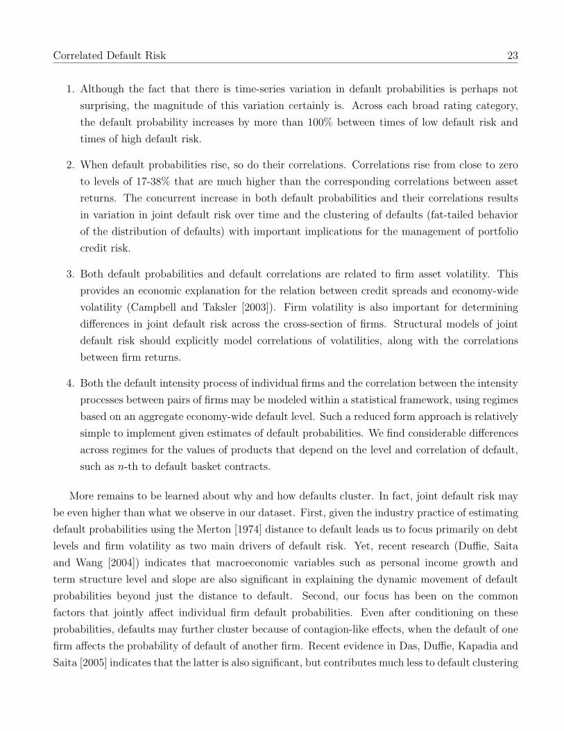
debt levels and firm volatilities vary across firms and over time.7 Exhibit 1 plots the median debt
(D/V ) and annualized firm volatility (σV ) across rated firms in the economy over the period 1987-
2000. We break our sample into three quality categories, where firms of Moody’s rating single-A
or higher are classified as high-grade, Ba and Baa are classified as medium-grade, and single-B and
C as low grade. The plot indicates that both debt and volatility have varied over this period. For
high-grade (low-grade) firms, the debt of the median firm ranges from 10.2% to 16.8% (32.3% to
48.4%), and volatility from 18% to 36.5% (29% to 45%). Debt levels across firms in the economy
appear to trend over time, while changes in volatility are more severe and tied to economic events.
Debt levels first increase over 1987 to 1991, then trend downward in the aftermath of the 1991-92
recession, and again trend upwards in the latter half of the 1990s. Volatility shows large increases
immediately after the 1987 crash, during the 1991-92 recession, and the latter half of the 1990s stock
market bubble that foreshadowed the bear market and subsequent recession of 2001-02. Excepting
the unlikely event that an increase in firm volatility is offset by a specific decline in debt level,
default probabilities of firms are not constant over time.
What is the relative impact of changes in debt and volatility on the probability of default of an
individual firm? Defining ∆ as the difference operator, observe from equation (1) that,
∆(DTD) ≈ −1
σV
√T
∆(D/V )− 1−D/V
σ2V T
∆(σV
√T ),
indicating that, at low debt levels, the DTD is more sensitive to changes in volatility than to
6For example, see footnote 8 in Sobehart and Stein’s [2000] description of the implementation of Moody’s RiskCalcmodel. In the Merton [1974] model, as the stock is priced using the risk-neutral distribution, the expected return ofthe firm is not required.
7To do so, we estimate debt ratio and firm volatilities across all firms in the Compustat-CRSP combined database.We first extract data for the period 1987-2000 on stock prices and debt per share. Using historical equity returnvolatilities for one year, we then invert the Merton [1974] model to obtain firm value V and firm volatility σV . Wesolve a system of two equations: one, which represents equity as a call option, and the other, the relationship ofequity volatility to firm volatility. This pair of equations contain two unknowns, V and σV which are easily solvedfor using standard numerical procedures. In our computations to estimate a one-year probability of default, we setT = 1, and D equal to the total of the face values of short term debt, and one-half of long term debt. We filterout firms whose volatilities are less than 0.1% or greater than 500%. Firms with debt ratio greater than 0.95 areconsidered to be in default, and also eliminated from the sample. Data on the one-year risk free interest rate isobtained from the Federal Reserve.

Correlated Default Risk 8
changes in debt levels. Over our sample period, the median high-grade (low-grade) firm had an
average volatility and debt of 24% (34%) and 11% (40%), respectively. At these volatility and debt
levels, consider the impact of an absolute change of 1% in either debt or volatility on the DTD.
For high grade firms, the impact of the change in volatility is 3.7 times the impact of the change in
debt value, and for low grade firms, it is 1.8 times. Thus, for the average firm in the economy, the
DTD is more sensitive to changes in volatility than changes in debt levels. In addition, over a short
horizon, volatility is often much more variable than debt levels, especially for high and medium
rated firms. As seen in Exhibit 1, volatility across the economy sharply increases in the aftermath
of the 1987 crash as well as in the latter half of the last decade.
Determinants of Default Probability Correlations
The correlation between PDs of two firms will depend on the correlation between the underlying
determinants of the default probabilities: correlation between individual firm debt levels, firm
returns, and firm volatilities. For example, Zhou [2001] derives the joint probability of default for
two firms when returns are correlated.
Exhibit 2 reports the median correlation between pairs of firms in our data. We classify our
sample by rating as well as by sub-period. The rating groups are as previously defined, and the
sub-periods are 1/87-6/90, 7/90-12/93, 1/94-6/97, and 7/97-10/00. We make the following obser-
vations. First, the median correlation between firms for each of these variables is positive. For
high grade and medium grade firms, the highest correlation is between the volatilities of firms.
For example, in the latest sub-period, the median correlation between volatilities for high-grade
(medium-grade) firms is 0.71 (0.35), while the median correlation between debt levels is 0.25 (0.26).
Second, differences between the rating classes appears to be driven mostly by differences in correla-
tion between volatilities. Across all sub-periods, the relative difference in median correlations across
all the three rating groups is the highest for the volatility correlations. Third, over time for each
rating class, correlations between firm returns are the most stable, while the correlations between
volatilities change the most. Interestingly, the correlations between volatilities are the highest in
the Periods I and IV when the level of volatility itself is high across the economy (see Exhibit 1).
Further Analysis
The results of the previous sections indicates that joint default risk will vary both over time and in
the cross-section of firms. However, these results do not allow us to quantify joint default risk. To do
so, we extend our dataset beyond the estimates from the Merton [1974] model. As Vassalou and Xing
[2004] note, the strict application of the Merton [1974] model generates default probabilities that do

Correlated Default Risk 9
not match actual aggregate default events in the economy. Instead, the standard approach in the
industry (e.g. EDF, RiskCalc) is to estimate a model for default probabilities econometrically using
a large dataset of default events and the DTD as an explanatory variable. The resultant estimates
of default probabilities are thus calibrated to match the aggregate level of historical defaults. For
this reason, Vassalou and Xing [2004] call the estimate from the Merton model a “default likelihood
indicator”, DLI. We shall follow their terminology to define the DLI as,
DLI = 1− Φ(DTD), (2)
and reserve the term PDs to refer to probabilities of default that have been calibrated to match
historical default levels.
Correlations of Default Probabilities
Default Probability Data
We obtain data on individual firms’ probabilities of default (“PDs’) ’from Moody’s Investors Ser-
vice through its subsidiary Moody’s Risk Management Services (“MRMS”). With their extensive
database of defaults, MRMS fits a model for short-term default risk using the distance to default
from the Merton [1974] model and additional financial statement information. The output from
their RiskCalc model is an estimate of a one-year default probability for an individual public firm at
a monthly frequency. Details of the model and its econometric fit are in Sobehart and Stein [2000].
The model uses as input firm-specific information: (a) company financial statement information (in-
cluding leverage, profitability, and liquidity measures), (b) the distance-to-default, and (c) Moody’s
ratings, if available. The use of information other than the distance-to-default is consistent with
the Merton model when asset values are not perfectly observable (Duffie and Lando [2001]).
The use of Moody’s PDs has important advantages in analyzing joint default risk. First, Moodys
calibrates their PDs to match the level of realized default; thus inferences about default correlations
are directly related to actual economy-wide joint default. If defaults are independent conditional
on PDs, then the correlations of PDs are also the correlations of default. This assumption of
conditional independence (see Jarrow, Lando and Yu [2005]) is a popular one in default models.
Second, the Moody’s PD uses the DTD as a co-variate for determining the probability of default.
Duffie, Saita and Wang [2004], for a subset of firms in the economy, demonstrate that changes in
the DTD has the greatest impact on determining changes in the probability of default. Sobehart
and Stein [2000] show that these PDs have predictive power, and perform as well, or better, than
alternative measures. Finally, we are able to find a consistent pattern of correlations relative to the
Moody’s data by creating our own data set of default likelihood indicators.

Correlated Default Risk 10
The data consists of a panel of monthly probabilities of default for North American non-financial
public firms over January 1987 to October 2000. The total number of unique firms that enter our
sample is 7,363. On any given date, the precise number of firms varies depending on new firm
inceptions, mergers, or defaults. For some of our analysis, we sub-divide our sample by period and
by rating classification. The four sub-periods include all firms that have continuous observations
within any of these sub-periods. The number of sub-periods is motivated by the trade-off between
having sufficient time series observations for estimation of correlation matrices, yet ensuring that
the period is relatively homogeneous so that differences in correlation matrices across sub-periods
may be observed. As noted earlier, the sub-periods are of almost equal length, and comprise the
periods, 1/87-6/90, 7/90-12/93, 1/94-6/97, and 7/97-10/00. As before, we group firms by credit
rating into three groups: high grade, medium grade and low grade. A firm is classified into a rating
class according to its average rating within the sub-period.
Exhibit 3 describes the data. The total number of unique firms range from 3,202 to 5,170 over
the sub-periods. The average number of firms in the high, medium and low grade groups are 215,
405 and 184, respectively. The vast majority of the firms in our sample are unrated, ranging from
2724 in Period I to 4142 in Period IV. The fraction of firms classified as high-grade declines from
over 6% in Periods I and II to about 4% in Period IV. This decline is offset mainly by an increase
in the fraction of firms classified as low grade. However, the fraction of firms in the two largest
categories - medium-grade and non-rated categories - is stable over time. As these two categories
together comprise about 90% of the total firms, the mix of firms across the economy is, for the most
part, stable over time.
As might be expected, the mean default probability increases monotonically as the average
rating declines, across each sub-period. For instance, the mean PD in Period IV is 0.23%, 1.17%
and 5.65% for high, medium and low grade firms, respectively. The mean PD of unrated firms is
in the range of 1.63% to 2.45%, suggesting that, if rated, these firms would fall in the lower rating
classes.
For comparison, we also form an industry grouping by SIC broad industry code. More than half
the firms in our sample belong to the manufacturing sector, Sector 4. The sector with the least
number of firms is Sector 1 (agriculture, forestry and fishing) with as few as 14 firms in Period II.
Although there is variation in PDs across sectors, this variation is small compared with that across
credit classes. Firms in sectors 1 and 5 have the lowest average PD, while firms in sector 10 have
the highest. The high default risk of sector 10 arises from firms of SIC group 99 (firms of industries
that cannot be classified into any of the other SIC groups).

Correlated Default Risk 11
Time Variation in Economy-Wide Default Probabilities
Two facts are immediately evident from Exhibit 3. First, there is considerable time-variation in
PDs across sub-periods. Second, the pattern of time-variation is consistent across all firms. Except
for firms in Sector 10, the mean default probability for groups of firms is the lowest in Period III
and highest in Period IV. If individual firm default probabilities change over time and these changes
are correlated, then this implies that the economy-wide default probability varies over time.
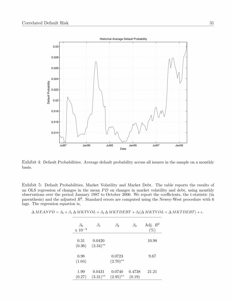
Exhibit 4 plots the monthly time series of the economy-wide probability of default, constructed
by averaging the default probabilities of individual firms, MEANPD(t) = 1N(t)
∑N(t)i=1 PDi(t), where
N(t) is the number of firms with a PD in month t. It is evident that the economy-wide probability
of default varies substantially at times. From our previous analysis, we expect the economy-wide
mean default probability to be related to economy-wide factors for volatility and debt. Comparing
Exhibit 4 with Exhibit 1, we, in particular, observe that the time-variation in the mean default
probability is closely related to the variation in firm volatilities. Each period of sharp increase in
the level of the economy-wide default probability corresponds to a period of sharp increases in firm
volatilities.
We verify the relative importance of debt and volatility at the aggregate level by a regression of
the economy-wide mean default probability on economy-wide factors for volatility and debt. Define
these to be the equal-weighted averages, MKTV OL(t) = 1N(t)
∑N(t)i=1 σV (t) and MKTDEBT (t) =
1N(t)
∑N(t)i=1 D(t)/V (t), where N(t) are the number of firms for which we have available data in month
t. Using a first-order linear approximation, we estimate the following OLS regression,
∆ MEANPD(t) = α + β1 ∆ MKTV OL + β2 ∆ MKTDEBT
+ β3( ∆ MKTV OL×∆ MKTDEBT ) + ε.
Exhibit 5 reports the results of the regression. We also report results for a subset of the variables
to allow for comparison. We can use the estimates of the coefficients to gauge the relative economic
importance of volatility and debt. Over the 166 months of our period, the average ∆MEANPD
is 1.05 basis points, while the average ∆MKTV OL and ∆MKTDEBT is 0.1828% and 0.0133%,
respectively. Given the estimated coefficients, the fraction of the average ∆MEANPD over the
166 months of our period explained by ∆MKTV OL and ∆MKTDEBT is 74.9% and 9.36%,
respectively. As expected from our previous analysis, the market-wide factor of volatility has a
larger economic impact on the time-variation in the economy-wide default probability.8 As market-
wide volatility is sensitive to economic conditions, the number of defaults in the economy is thus
tightly linked to the state of the economy.
8This conclusion is consistent with Campbell and Taksler’s [2003] recent finding that corporate bond spreads arecorrelated with volatility.

Correlated Default Risk 12
Empirical Evidence on Default Intensity Correlations
We next analyze how default correlations (defined below) vary over time and in the cross-section.
To do so, we first convert the one-year default probability into a corresponding default intensity,
λi = − ln(1− PDi), (3)
where λi is the constant default intensity that corresponds to the 1-year default probability PDi.9
This eliminates the maturity dependence from our data, and also allows our results to be interpreted
within the framework of reduced form models (see Jarrow and Turnbull [1995], Madan and Unal
[1998], Duffie and Singleton [1999] and Duffie and Lando [2001]).
We examine the correlation between default intensities using two models. First, we compute the
correlations between changes in default intensities. Let
λi(t)− λi(t− 1) = εi(t), (4)
then the correlation between default intensities of firms i and j, ρij, is the correlation between εi
and εj over this period.
In our second model, we model the default intensity as a discrete time AR(1) process,
λi(t) = αi + βiλi(t− 1) + εi(t). (5)
The correlation between firms i and j is the correlation between εi and εj. The model of equation
(5) is a mean-reverting intensity processes as used in the reduced form literature (Duffee [1999]).
When we estimate the model across the firms in our database, the median βi ranges from 0.90 to
0.94 across the rating classes and sub-periods.
We report both the usual Pearson correlation as well as the rank correlation. There are two
reasons for reporting the rank correlation. First, the rank correlation imposes less stringent condi-
tions on the data as the results are valid even if default intensities, like ratings, only order firms on
the dimension of default risk. Second, the use of the rank correlation ensures that the results and
conclusions of this section are applicable to other measures of default risk that are not necessarily
calibrated to the actual level of defaults in the economy, but simply rank firms by their default
probabilities. For example, these results also hold if the distance-to-default from the Merton model
is used as an ordinal measure of default risk.
9The transformation of PDs to default intensities is based on the assumption that intensity process is constant.As a check, for a number of firms, we also derive the instantaneous intensity process by modeling it as an affinemodel of the CIR form. The correlation of the resultant intensity process under the two separate transformations isclose to 1. See also the discussion in Das, Duffie, Kapadia and Saita [2005]. Thus, given the objectives of this paper,we choose to work with the constant intensity process.
Correlated Default Risk 13
We compute the correlations for every pair of firms in our sample for sub-samples of our data,
and the median of the pair-wise correlations is reported in Exhibit 6. Panel A reports the statistics
for the quality groups, and Panel B for the industry sectors. We report the following findings.
First, the median default correlation is non-negative across all credit classes and in every period.
This result holds for both models of the default intensity process, equation (4) or equation (5), as
well as whether the correlation coefficient is computed as the Pearson or as the rank correlation.
For the model of equation (4), the magnitude of the Pearson coefficient ranges from 0.02 to 0.37.
When computed from the residuals of equation (5), the correlation coefficients are of similar mag-
nitude. That the median correlation is positive across all sub-samples is consistent with our earlier
observation that default probabilities are affected by an economy-wide volatility factor.
Second, default intensities of high grade firms are more highly correlated than firms of lower
rating classes. This conclusion is also robust across both models and measures of correlation coeffi-
cient. The difference between rating classes is particularly high in Periods I and IV. For example, in
Period I, the median Pearson correlation computed from equation (5) is 0.37 for high-grade firms,
compared with 0.23 and 0.16 for medium- and low- grade firms. Non-rated firms have correla-
tion coefficients similar to those of medium- and low-grade firms. The observation that default
probabilities of high-grade firms are more highly correlated, and especially so in Periods I and IV,
follows the pattern previously observed for asset return volatilities in Exhibit 2. Using data on
credit spreads, Xiao [2003] observes that changes in credit spreads of high grade bonds are also
more highly correlated than credit spreads of lower rated bonds.
Third, the median correlation within each group varies over the sub-periods. The striking
pattern that can be observed in Exhibit 6 is that the time-variation in correlations is consistent
across sub-groups. Across all rating classes, the correlations are highest in Periods I and IV, and
lower in Periods II and III. For each of the rating classes, the lowest Pearson correlation for Model
1 is close to zero in Period III, but increases to a range of 16-36% in Period IV. Once again, the
pattern of time-variation in correlations of default intensities is closest matched in Exhibit 2 by the
pattern of variation in the correlations between firm volatilities. This similarity also extends to the
cross-sectional differences in the magnitude of time-variation of correlations. High-grade firms have
the greatest variability in correlations of both asset return volatilities and default intensities, and
low-grade firms show the least.
Panel B of Exhibit 6 reports the results when firms are classified into industry sectors. Median
correlations are, once again, predominantly positive. As with rating classes, correlations are time-
varying, with correlations in Periods I and IV higher than in Periods II and III across almost all
sectors. With the sole exception of sector 10 (Public Administration), the lowest median correlation
is in Period III. Thus, the time variation of correlations appears to be systematic across the firms,

Correlated Default Risk 14
irrespective of how firms are classified.
We provide two alternative sets of results that, although of independent interest, also serve
as robustness tests. First, as an alternative to considering pair-wise correlations, we analyze the
principal components of the residuals from Equation (4) and Equation (5). Exhibit 7 reports the
fraction of the variance of the residuals explained by the first, and the top two principal components,
respectively. The results indicate that the primary cross-sectional and time-series conclusions of
Exhibit 6 are robust. In Periods I and IV, the first two components explain more than twice the
variance for high grade firms than for lower grades. Overall, the conclusions from Exhibit 7 are
consistent with those of Exhibit 6.
We also report correlations across rating classes for the Merton DLI of equation (2). The use
of the DLI helps us to verify that the results are not dependent on the specific econometric model
used to calibrate the default probabilities. Exhibit 8 reports the results. Although the magnitude
of the median correlation is lower as compared with Model 1 in Exhibit 6 (as estimates of default
probabilities include additional factors besides the DLI), the correlations nevertheless exhibit the
same patterns in the cross-section and time-series.
An important conclusion that emerges from the results of this section is that both the time-
variation in default intensities as well as time-variation in the correlation between default intensities
are of substantial magnitude. More importantly, as increases in default probabilities appear to
coincide with increases in default correlations, both these effects will result in substantial variation
in the economy-wide default risk.
Modeling Time-Variation in Default Probabilities and De-
fault Correlations
In this section, we propose a statistical model that explicitly accounts for systematic time-variation
in both default probabilities and their correlations. Empirical evidence of the previous sections
indicates that economy-wide levels of default risk, default correlations and volatility are related to
each other. Increases in volatility lead to increases in the economy-wide default level as well as
increases in the correlations of default intensities. We directly model this link between economy-
wide default risk and the magnitude of correlations through a Hamilton [1989] type regime-shifting
model with different correlations across regimes. A comparison of sub-period IV (high default risk,
high correlations) versus sub-period III (low default risk, low correlations) suggests that a two-
period regime-switching model is a likely candidate for good fit. Similar time-varying correlation
models have been proposed in Erb, Harvey and Viskanta [1994], Longin and Solnik [1995] and Ang
and Chen [2002] for modeling time-varying and asymmetric equity correlations.

Correlated Default Risk 15
Determining Regimes for Default Intensities
We estimate a two-regime model for default risk in the economy. Let the average (across all issuers)
default intensity, denoted by λ(t) =[
1N(t)
∑N(t)i=1 λi(t)
], follow an AR(1) model that depends on the
prevailing regime, kt ∈ 1, 2, at time t (we will suppress the subscript on kt below):
λ(t)− θk = βk[λ(t− 1)− θk] + vkzt
Regimes kt =
1 high default regime2 low default regime
where zt has a standard normal distribution. kt follows a Markov chain with a transition matrix,(q1 1− q1
1− q2 q2
), where q1 and q2 are the transition probabilities, for s > t, q1(s, t) = Pr(ks =
1 | kt = 1) and q2(s, t) = Pr(ks = 2 | kt = 2). The mean reversion rate, 1 − βk, the mean default
rate, θk, and the volatility vk are regime dependent. The discrete transition density is
f [λ(s) | λ(t)] = exp
(−(λ(s)− λ(t)− (1− βk)(θk − λ(t)) )2
2(vk)2
)1√
2π(vk)2. (6)
We write the Markov probabilities at time t in logit form as,
qkt(s, t) =exp
(ak + bkxt
)1 + exp(ak + bkxt)
, kt = 1, 2 (7)
where xt is a state variable that impacts the transition probability, and ak and bk are transi-
tion function parameters to be estimated. Here, we allow for the possibility that the transition
probabilities may vary over time with the short rate (xt = rt), or with average firm volatility
(xt = MKTV OL(t)), or be constant, i.e. bk = 0. As we expect regimes, if any, to be correlated
with the economic events, the short-rate and volatility are natural candidates for determining tran-
sition probabilities. The standard Hamilton approach is used to fit the following objective function:
β1, β2, θ1, θ2, v1, v2, a1, a2, b1, b2∗ = arg maxT∑
t=1
log[f(λt)]. (8)
Maximum likelihood estimates for the model are presented in Exhibit 9.10 Panel A provides
the estimates under the assumption of constant transition probabilities, bk ≡ 0. The mean level of
10The specifications for intensities in this and the next subsection do not preclude negative intensities. A loga-rithmic specification (that ensures positive intensities) did not converge for the regime-switching estimation model.However, the parameter estimates for the volatility vk in both regimes in comparison to the mean values of intensitiesθk shows that the probability of negative intensities is extremely negligible.
Correlated Default Risk 16
default in regime 1 (θ1 = 1.77%) is more than twice that of regime 2 (θ2 = 0.74%). The volatility, vk,
is also higher in regime 1 versus regime 2 (0.07% vs. 0.04%). The probability parameter (ak) results
in high values of qk, suggesting strong persistence in each regime. The probability of remaining in
regime 1 is lower (0.8765) than the probability of remaining in regime 2 (0.9692). Raising the
transition matrix to the power of infinity provides the long-run stable probabilities of each regime,
which are roughly 20% in the regime 1 and 80% in regime 2. All estimates are statistically significant
in Panel A. Panel B and C reports the estimates where the transition probabilities are allowed to
be state-dependent. The coefficient bk is insignificant in both panels, and therefore, the results are
economically similar to those in Panel A.
The parameter estimates across the two regimes identify regime 1 (2) as a regime with high (low)
mean default rates and volatility. In Exhibit 10, the probability of being in regime 1 is presented for
the time period spanned by the data set. The probabilities track the patterns originally observed
in Exhibit 4, indicating, in particular, the existence of high/low default rate regimes.
Regime-Dependent Parameters for Rating Classes
In the previous sub-section, we determined the two regimes within our sample period in terms of
the process for the average level of default in the economy. Next, we look at how the parameters
of the intensity process vary across these two regimes for the average firm in each rating class. We
identify a specific time period as being of regime 1 (High) or 2 (Low), if the probability of being
in that regime is more than 0.5 (see Exhibit 10). Of the 166 month period from January 1987 to
October 2000, 30 months are identified as being in regime 1.
Using the defined regimes, we estimate the parameters for each rating class in each regime. We
model the rating level default intensity
λki (t) =
1
Ni(t)
Ni(t)∑j=1
λkij(t)
as follows, where we use i to index the rating class and j to index a firm within a rating class.
λki (t) = λk
i (t− 1) + (1− βki )[θk
i − λki (t− 1)
]+ vk
i εi(t), k ∈ 1, 2. (9)
Assuming a standard normal distribution for εi(t), the parameters are estimated by maximum
likelihood,
maxΩ
T∑t=1
ln F [λki (t)], (10)
where Ω = βki , θk
i , vki , k ∈ 1, 2.
F [λki (t)] = 11 × f [λ1
i (t)] + 12 × f [λ2i (t)], (11)

Correlated Default Risk 17
and f [λki ] is the conditional density for the stochastic process in equation 9 and 1k are indicator
functions based on the regimes identified in the previous subsection.
The results in Exhibit 11 show clearly that the mean default rate is different in the two regimes
for every class. Mean default rates (θki ) increase by 127%, 261% and 102%, for the high, medium
and low grade firms, respectively. Volatilities (vki ) also increase in the high regime, and as credit
quality declines. The difference in the volatility between the two regimes differs by credit class, with
the lowest credit class showing little difference across regimes, in contrast to a three-fold increase
for the highest rating class. For each rating class, the rate of mean reversion, (1 − βki ), is also
different across the two regimes, and is higher in regime 1. Mean reversion increases as credit
quality decreases.
Overall, the regime-dependent parameters for the average firm in each class show similar patterns
as those identified earlier for the overall default level of the economy.
Issuer correlations across regimes
For firms in each rating class, we compute the covariance matrix of Model 2 (equation 5) residuals
in each of the two regimes, and test for differences in covariances across regimes using the following
test.11 Let Sk, k = 1, 2 be the covariance matrix for each regime k. The null hypothesis is that
the covariance matrices are equal across the two regimes, i.e. S1 = S2. To construct the test, define
Ck =Sk
nk − 1,
where nk, k = 1, 2, are the number of observations used to compute each covariance matrix.
Compute the pooled covariance matrix as follows:
C =
∑k(n
k − 1)Ck
n−m, k = 1, 2
where n =∑
k nk, and m = 2 (testing for the equality of only 2 covariance matrices). The null
hypothesis of equality of the covariance matrices is tested using a modified log-likelihood ratio
statistic L,
L = M × h,
M = (n−m) ln |C| −∑k
(nk − 1) ln |Ck|,
11There are several useful references to this class of test. The simplest source is fromhttp://www.gseis.ucla.edu/courses/ed231a1/notes3/covar.html. See also Takemura, Akimichiand Kuriki, Satoshi - “Maximum Covariance Test for Equality of Two Covariance Matrices” -University of Tokyo, and The Institute of Statistical Mathematics. See also the SAS code inhttp://ewe3.sas.com/techsup/download/stat/CovMxTest.html.
Correlated Default Risk 18
h = 1− 2p2 + 3p− 1
6(p + 1)(m− 1)
(∑k
1
nk − 1− 1
n−m
),
where p is the dimension of the covariance matrix, and L is distributed χ2[p(p + 1)(m− 1)/2]. If L
exceeds the critical value, then we reject the hypothesis that the covariance matrices are equal.
Results are presented in Exhibit 12 on a random sample of 30 firms in each rating category. For
each of the three rating categories, we can easily reject the hypothesis that covariance matrices are
equal across the two regimes. Thus, the results suggest that correlations are, indeed statistically
different between regimes.
In addition, we also considered the fraction of the variance explained by the first principal
component in each regime across each rating class. In the high default regime, the fraction explained
by the first principal component is 61%, 55% and 69% for high, medium and low grade firms,
respectively. In contrast, the fraction explained by the first principal component in the low default
regime is 32%, 34% and 35% for each rating class, respectively. Overall, the evidence indicates the
correlations across the two regimes are different, with the correlation, on average, being higher in
the high-default regime as compared with the low-default regime.
The evidence in this section indicates that a statistical regime-shifting model is able to capture
both the time-variation in default probabilities and correlations that were observed in the previous
sections. The regimes are based on the economy-wide level of default probability, and thus accounts
for the two observations that the changes in joint default risk are systematic, and that changes in
both the level of the default probability and default correlations are related to common factor(s).
Because the implementation of the model does not require any additional information beyond the
time-series of default probabilities, it can be easily implemented.
In the next section, we provide applications that use the analysis of this and the previous sections
to quantify the differences in regimes in terms of the likelihood of (joint) default across a portfolio
of firms.
Analysis
In this section, we provide two numerical examples to assess the economic importance of our findings.
We do so using standard factor copula techniques that are widely used by practitioners. First, we
compute n’th to default probabilities to illustrate the differences across regimes. As the probability
of the n’th default from a basket of issuers is sensitive to both the levels of the default intensity
as well as the correlations between the intensities, these probabilities are a good way to illustrate
the economic importance of the regimes detected earlier. Second, we examine the economic impact

Correlated Default Risk 19
of changing economic conditions. We quantify the tails of the distribution of defaults over a large
portfolio of firms, and ask how unusual it is to observe the economy-wide level of defaults in 2001.
N’th to Default Probability
Consider the computation of the probability of exactly n defaults from a credit basket of m ≥ n
bonds.12 These probabilities are sensitive to both the level of default and the degree of correlation
between the issuers, and allow us to quantify the effects of both in a simple one-period model.
Let each bond have a distinct issuer i, whose default risk is characterized by a default intensity,
λi = θi + v∗i xi, where θi is the mean intensity, and v∗i is the unconditional standard deviation. The
variable xi consists of a random shock which is a function of a latent factor deviation Y , common
across all issuers, with constant cross-sectional correlation ρ, and an idiosyncratic component εi, i.e.
xi = ρY +√
1− ρ2εi,
εi ∼ N(0, 1),
Y ∼ (µY , σ2Y ).
The variables Y and εi are uncorrelated, as are the εis. This specification injects the required
correlation amongst the intensities for each issuer through the common component Y .
Assuming unit time, the survival probability is equal to si = e−λi , and therefore, the expected
survival probability, conditional on Y , is
si(Y ) = E[exp(−λi)|Y ]
= E exp[−(θi + v∗i xi)]
= Eexp[−(θi + v∗i [ρY +
√1− ρ2εi])]
= exp
−θi − v∗i ρY +
(v∗i )2
2(1− ρ2)
. (12)
Likewise, the expected conditional default probability is pi(Y ) = 1− si(Y ).13
12Laurent and Gregory [2003] provide a very nice overview of this class of products. See Duffie and Garleanu [2001]for the pricing of CDOs.
13For m bonds, assuming Y is normally distributed, the expected number of defaults may be shown (after somelengthy though simple calculations) to be equal to
E(n) =
∫Y
m∏i=1
si(Y ) dY
= m − exp
[(m∑
i=1
(v∗i )2
)(1− ρ2)−
(m∑
i=1
θi
)−
(m∑
i=1
v∗i
)ρµY +
1
2
(m∑
i=1
v∗i
)2
ρ2σ2Y
]
Correlated Default Risk 20
In order to examine the probability distribution of the number of defaults, we use probability
generating functions, implementing the ideas previously developed in papers by Finger [1999], Mina
and Stern [2003], and Gregory and Laurent [2004]. We denote the probability of n defaults from m
bonds in unit time as p(n). From m issuers, n can take values in the set 0, 1, 2, ...,m. Conditional
on Y , the probability of n defaults is denoted p(n|Y ). We define the probability generating function
of p(n) as g(t|Y ) conditional on Y :
g(t|Y ) =m∑
n=0
p(n|Y )tn, 0 ≤ t ≤ 1
= p(0|Y ) + p(1|Y )t + P (2|Y )t2 + ... + p(m|Y )tm, (13)
where t is the parameter of the probability generating function (pgf). For each individual issuer i,
the pgf is as follows:
gi(t|Y ) = pi(0|Y ) + pi(1|Y )t
= 1− pi(Y ) + pi(Y )t
= si(Y ) + (1− si(Y ))t. (14)
Conditional on Y , the pgf of each issuer is independent of the other issuers, and we may write the
joint pgf as:
g(t|Y ) =m∏
i=1
gi(t|Y ),
=m∏
i=1
[si(Y ) + (1− si(Y ))t] , 0 ≤ t ≤ 1. (15)
which is calculated using equation (12). We let t ∈ 0, 1/m, 2/m, ..., 1, this represents (m + 1)
equations, one for each t. This calculation provides the LHS value for the system of equations in
(13), which then contains (m + 1) probabilities p(n|Y ), which may be solved for using a simple
matrix inversion. By integrating out Y , we obtain
p(n) =∫
Yp(n|Y ) dY
These are precisely the values we are interested in, i.e. the probability density function for the
number of defaults n.
For illustration, we set the number of issuers m equal to 10. We assume that the factor deviation
Y is standard normal. We use parameters values βi, θi and vi from Exhibit 11. In this one-period
model, we obtain the unconditional standard deviation of intensities from the table, and denote
Correlated Default Risk 21
them v∗i , where v∗i is set to
√v2
i
2(1−βi), approximating unconditioning. The correlations corresponding
to the high and low default regimes are the median correlation from Period III and IV, respectively,
in Exhibit 6. Using the procedure outlined above, we compute the values of p(n), n = 0...m, across
regimes and rating classes. Our goal is to examine the difference in these distributions across regimes
for each rating class.
The results are presented in Exhibit 13. The difference in the distributions across the two
regimes is apparent. For example, the probability of observing a default in a portfolio of 10 high-
grade firms is 2.47% in the high default regime, more than twice the probability in the low-default
regime. Even more striking is the difference in the tails of the distributions for larger number of
defaults - the probabilities of default in the high-default regime are a large multiple of the values in
the low regime (although limitations on the number of decimals that we can report in Exhibit 13
does not always make it apparent).
The procedure outlined above for the implementation of the n-th to default model is extendable
to a much larger basket of bonds. As an illustration, we extended the approach to m = 100
bonds. The integration of the probabilities in this approach is undertaken using a Fourier transform
approach instead, which speeds up the computations. Using the same parameters as in Exhibit 13,
we generated the distribution of probabilities for n out of m defaults, i.e. p(n). For the high default
risk regime, the probability density functions for all three rating classes are presented in Exhibit
14. The plots for the low default risk regime are also plotted in the same Exhibit. The tails of the
distribution are larger in the high risk regime. In the low rating class, there is a 5% probability of
11 or more defaults in the high default regime, whereas in the low default regime, there is a 5%
probability of only 7 or more defaults.
Impact of Changing Economic Conditions
In this next illustration, rather than use average parameter estimates, we use default intensity data
across the firms in our dataset to examine the economic impact of changing economic conditions
across a large portfolio of firms. To do so, we first combine data from sub-periods I and IV to
comprise a “high” default risk regime, and data from sub-periods II and III to form a “low” default
risk regime. We then form portfolios of firms that have data across all months in our sample. The
number of firms in each rating category in our analysis are 114, 238 and 106 for the high, medium
and low rating classes respectively.14
Within each regime and rating class, using the raw intensity data, we compute the vector of
14The number of firms is less than that totally available in each subperiod (see Exhibit 3) because we have combinedsubperiods and only used firms with full data across subperiods.
Correlated Default Risk 22
mean intensities for all firms and the covariance matrix. Assuming that intensities are lognormal,15
and a horizon of one year, we can compute the distribution of aggregate intensity (denoted A) for
each rating class. The probability of n defaults (assuming independence across defaults conditioned
on A) is denoted p(n|A). To obtain the probability of n defaults, we then integrate, i.e.
p(n) =∫
Ap(n|A)f(A)dA, ∀n,
where f(A) is the probability density function for A, and p(n|A) is Poisson with parameter A.
Computing p(n) for all n results in the probability function for the number of defaults.
In Exhibit 15, we present the difference in probability functions between the high and low
regimes. The PDF of the low regime is subtracted from the PDF for the low regime. This is done
for each of the three rating classes. We observe that the tail of the distributions is much fatter in
the high default regime.
To gain a sense of the economic impact of the differences across these two regimes, consider the
low rating class in both regimes, as a proxy for the High-Yield debt market. We plot in Exhibit
16 the cumulative default probability of the number of defaults of the 106 firms in that category
in each regime. To fix ideas, consider the fact that the default rate in the High-Yield Sector in
2001 was about 10% - at a historical peak. This would be about 11 firms or more in our sample
defaulting in about one year (recall that our sample period ends in October 2000). In Exhibit 16
we have plotted a vertical line at this number of firms. We can see that the probability of reaching
or surpassing this level of default is less than 10% in the low regime, but is more than twice in
the high regime - there is a 1-in-5 chance of seeing the default levels of 2001. In summary, when
one models joint changes in default probabilities and default correlations across regimes, the high
number of defaults observed in 2001 is not a low probability event.
Concluding Comments
In this paper, we document how the correlation of default probabilities varies both in the cross-
section of firms and over time. Our primary conclusion is that joint credit risk varies because both
default probabilities and default correlations vary with economic conditions. Moreover, market-wide
volatility plays an important role in determining this time-variation in joint default risk. Clustering
of defaults occurs during times of high volatility, and does so because both default probabilities and
correlation between defaults increase.
We provide below a summary of our findings and their implications:
15Since the analysis is based on raw data, the choice of lognormal joint distribution for the intensities ensurespositive values. Any other joint distribution with positive support over intensity values is also possible.
Correlated Default Risk 23
1. Although the fact that there is time-series variation in default probabilities is perhaps not
surprising, the magnitude of this variation certainly is. Across each broad rating category,
the default probability increases by more than 100% between times of low default risk and
times of high default risk.
2. When default probabilities rise, so do their correlations. Correlations rise from close to zero
to levels of 17-38% that are much higher than the corresponding correlations between asset
returns. The concurrent increase in both default probabilities and their correlations results
in variation in joint default risk over time and the clustering of defaults (fat-tailed behavior
of the distribution of defaults) with important implications for the management of portfolio
credit risk.
3. Both default probabilities and default correlations are related to firm asset volatility. This
provides an economic explanation for the relation between credit spreads and economy-wide
volatility (Campbell and Taksler [2003]). Firm volatility is also important for determining
differences in joint default risk across the cross-section of firms. Structural models of joint
default risk should explicitly model correlations of volatilities, along with the correlations
between firm returns.
4. Both the default intensity process of individual firms and the correlation between the intensity
processes between pairs of firms may be modeled within a statistical framework, using regimes
based on an aggregate economy-wide default level. Such a reduced form approach is relatively
simple to implement given estimates of default probabilities. We find considerable differences
across regimes for the values of products that depend on the level and correlation of default,
such as n-th to default basket contracts.
More remains to be learned about why and how defaults cluster. In fact, joint default risk may
be even higher than what we observe in our dataset. First, given the industry practice of estimating
default probabilities using the Merton [1974] distance to default leads us to focus primarily on debt
levels and firm volatility as two main drivers of default risk. Yet, recent research (Duffie, Saita
and Wang [2004]) indicates that macroeconomic variables such as personal income growth and
term structure level and slope are also significant in explaining the dynamic movement of default
probabilities beyond just the distance to default. Second, our focus has been on the common
factors that jointly affect individual firm default probabilities. Even after conditioning on these
probabilities, defaults may further cluster because of contagion-like effects, when the default of one
firm affects the probability of default of another firm. Recent evidence in Das, Duffie, Kapadia and
Saita [2005] indicates that the latter is also significant, but contributes much less to default clustering
Correlated Default Risk 24
than the co-movement of default probabilities. This paper has developed a basic understanding of
joint default risk, and motivates a further exploration of the clustering of defaults.
References
[2002] Allen, L., and A. Saunders (2002). “A Survey of Cyclical Effects in Credit Risk Measurement
Models,” working paper, New York University.
[2002] Altman, Edward. I., Brooks Brady, Andrea Resti, and Andrea Sironi (2002). “The Link
Between Default and Recovery Rates: Implications for Credit Risk Models and Procyclicality,”
forthcoming, Journal of Business.
[2002] Ang, A., and J. Chen (2002). “Asymmetric Correlation of Equity Portfolios,” Journal of
Financial Economics, v63(3), 443-494.
[1973] Black, F., and M. Scholes (1973) “The Pricing of Optionsand Corporate Liabilities,” Journal
of Political Economy, v81,637-654.
[2003] Campbell, John., and Glen Taksler (2003). “Equity Volatility and Corporate Bond Yields,”
Journal of Finance, v58, 2321-2349.
[2003] Collin-Dufresne, P., R. Goldstein, and J. Helwege (2003). “Is Credit Event Risk Priced?
Modeling Contagion via the Updating of Beliefs,” working paper, Haas School, University of
California, Berkeley.
[2001] Collin-Dufresne, P., and B. Goldstein (2001). “Do Credit Spreads Reflect Stationary Leverage
Ratios?,” The Journal of Finance, v56(5).
[2005] Das, S., D. Duffie, N. Kapadia and L. Saita (2005). “Common Failings: How Corporate
Defaults Cluster,” forthcoming Journal of Finance.
[2001] Das, S., G. Fong., and G. Geng (2001). “The Impact of Correlated Default Risk on Credit
Portfolios,” Journal of Fixed Income, December 2001, v11(3), 9-19.
[2004] Das, Sanjiv., and Gary Geng (2004). “Correlated Default Processes: A Criterion-Based
Copula Approach,” Journal of Investment Management, v2(2), 44-70.
[1996] Das, S., and P. Tufano (1996). “Pricing Credit Sensitive Debt when Interest Rates, Credit
Ratings and Credit Spreads are Stochastic,” The Journal of Financial Engineering, v5(2),
161-198.

Correlated Default Risk 25
[2000] Das, S., and R. Sundaram (2000). “A Discrete-Time Approach to Arbitrage-Free Pricing of
Credit Derivatives,” Management Science, v46(1), 46-62.
[2001] David, Mark., and Violet Lo (2001). “Infectious Defaults,” Quantitative Finance, v1(4),
382-387.
[2002] de Servigny, Arnaud., and Olivier Renault (2002). “Default Correlation: Empirical Evi-
dence,” working paper, Standard & Poors.
[2002] Driessen, Joost (2005). “Is Default Event Risk Priced in Corporate Bonds?” Review of
Financial Studies 18, 165-195.
[2001] Duffie, D. and Garleanu, N (2001). “Risk and Valuation of Collateralized Debt Obligations,”
Financial Analysts Journal, Vol. 57(1), (January-February), 41-59.
[2001] Duffie, Darrell., and David Lando (2001). “Term Structure of Credit Spreads with Incomplete
Accounting Information” Econometrica, v69, 633-664.
[1999] Duffie, D. and Singleton, K (1999). “Modeling Term Structures of Defaultable Bonds,” Re-
view of Financial Studies, Vol. 12(4), (Special), 687-720.
[2004] Duffie, Darrell., Leandro Saita and Ke Wang (2004). “Multi-Period Corporate Default Pre-
diction with Stochastic Covariates”, Graduate School of Business, Stanford University..
[1999] Duffee, G (1999). “Estimating the price of default risk,” Review of Financial Studies 12,
197-226.
[1994] Erb, Claude., Campbell Harvey, and Tadas Viskanta (1994). “Forecasting International Eq-
uity Correlations,” Financial Analysts Journal, November/December, 32-45,
[1999] Finger, Chris (2004). “Conditional Approaches for CreditMetrics Portfolio Portfolio Distri-
butions,” CreditMetrics Monitor, April, 14-33.
[2002] Giesecke, Kay (2002). “Correlated Default with Incomplete Information,” working paper,
Humboldt University, Berlin.
[2004] Gregory, Jon and Jean-Paul Laurent (2004). “In the Core of Correlation,” unpublished
manuscript.
[1989] Hamilton, J.D. (1989), “A New Approach to the Economic Analysis of Nonstationary Time
Series and the Business Cycle,” Econometrica, 57, 357-384.
Correlated Default Risk 26
[1995] Jarrow, R and S. Turnbull (1995). “Pricing Derivatives on Financial Securities subject to
Credit Risk,” Journal of Finance v50[1] (March), 53-86.
[1997] Jarrow, R., D. Lando, and S. Turnbull (1997). “A Markov Model for the Term Structure of
Credit Spreads,” Review of Financial Studies, v10, 481-523.
[2005] Jarrow, R., D. Lando, and F. Yu (2005), “Default Risk and Diversification: Theory and
Empirical Implications,” Mathematical Finance, v15(1), 1-26.
[2001] Jarrow, R., and Fan Yu (2001). “Counterparty Risk and the Pricing of Defaultable Securi-
ties,” Journal of Finance, v56(5), 1765-1799.
[2003] Laurent, Jean-Paul, and Jon Gregory (2003). “Basket Default Swaps, CDOs and Factor
Copulas,” working paper, ISFA Actuarial School and University of Lyons.
[1996] Leland, Hayne., and Klaus Toft (1996). “Optimal Capital Structure, Endogenous
Bankruptcy, and the Term Structure of Credit Spreads,” Journal of Finance, v51(3), 987-1019.
[1995] Longin, F., and B. Solnik (1995). “Is the Correlation in International Equity Returns Con-
stant: 1960-1990?” Journal of International Money and Finance, v14, 3-26.
[1995] Longstaff, F., and Schwartz, E. (1995), “A Simple Approach to Valuing Risky Fixed and
Floating Rate Debt,” Journal of Finance, Vol. 51[3] (September), 789-819.
[2002] Lopez, Jose, A. (2002). “The Empirical Relationship between Average Asset Correlation,
Firm Probability of Default and Asset Size,” working paper, Federal Reserve Bank of San
Francisco.
[1995] Lucas, D. J. (1995). “Default Correlation and Credit Analysis,” The Journal of Fixed Income,
March, 76-87.
[1998] Madan, Dilip and H. Unal, (1998). “Pricing the Risks of Default,” Review of Derivatives
Research, v2 (2/3), 121-160. 449-470.
[1974] Merton, R. (1974). “On the Pricing of Corporate Debt: The Risk Structure of Interest
Rates,” Journal of Finance, v29, 449-470.
[2003] Mina, Jorge, and Eugene Stern (2003). “Examples and Applications of Closed-Form CDO
Pricing,” RiskMetrics Journal, v4(1), 5-34.
[2004] Schonbucher, Philipp (2004) “Frailty Models, Contagion, and Information Effects,” Working
Paper, ETH, Zurich.

Correlated Default Risk 27
[2000] Sobehart, J., R. Stein (2000). “Moody’s Public Firm Risk Model: A Hybrid Approach
To Modeling Short Term Default Risk,” Moody’s Investors Service, Global Credit Research,
Rating Methodology, March.
[2004] Vassalou, Maria, and Yuhang Xing (2004). “Default Risk in Equity Returns,” The Journal
of Finance, v59(2), 831-868.
[2003] Xiao, Jerry (2003). “Constructing the Credit Curves: Theoretical and Practical Considera-
tions,” working paper, RiskMetrics.
[2003] Yu, F. (2003). “Default Correlations in Reduced Form Models,” forthcoming, Journal of
Investment Management.
[2001] Zhou, C. (2001). “An Analysis of Default Correlations and Multiple Defaults,” Review of
Financial Studies 14, 555-576.
Correlated Default Risk 28
Jul87 Jan90 Jul92 Jan95 Jul97 Jan00
0.15
0.2
0.25
0.3
0.35
0.4
0.45
Date
D/V
Firm Debt from 1987!2000
High GradeMedium GradeLow Grade
Jul87 Jan90 Jul92 Jan95 Jul97 Jan00
0.2
0.25
0.3
0.35
0.4
0.45
Date
Firm volatility from 1987!2000
High GradeMedium GradeLow Grade
Exhibit 1: Debt and Volatility over 1987-2000. The plot graphs the median debt fraction (D/V ) andthe firm return volatility (σV ) of firms in each rating category for each of the 166 months over the periodJanuary 1987 to October 2000. The firm value and the firm return volatility are estimated on a monthlyfrequency using Merton (1974). The debt is measured as the sum of current debt plus half the long-termdebt. Firms with Moody’s rating single-A or higher are classified as high-grade, Ba and Baa are classifiedas medium-grade, and single-B and C as low grade.

Correlated Default Risk 29
Exhibit 2: Correlations of Firms’ Return, Debt and Volatility. The table reports correlations of (i) returnson firm value, (ii) debt fraction (D/V ) and (iii) volatility (σV ) across firms in each rating class. Firmvalue and return volatilities are computed using the Merton model with data from Compustat and CRSP.Correlations are computed for every pair of firms in the class. The median of all pair-wise correlations isreported in the table. Firms with Moody’s rating single-A or higher are classified as high-grade, Ba andBaa are classified as medium-grade, and single-B and C as low-grade. The four sub-periods are: 1/87-6/90,7/90-12/93, 1/94-6/97, and 7/97-10/00.
Group Period I Period II
Correlation of Correlation ofReturn Debt Volatility Return Debt Volatility
High Grade 0.13 0.12 0.85 0.08 0.06 0.27
Medium Grade 0.10 0.10 0.59 0.06 0.12 0.15
Lower Grade 0.05 0.10 0.19 0.03 0.20 0.13
Group Period III Period IV
Correlation of Correlation ofReturn Debt Volatility Return Debt Volatility
High Grade 0.05 0.07 0.10 0.07 0.25 0.71
Medium Grade 0.05 0.02 0.07 0.07 0.26 0.35
Lower Grade 0.04 0.05 0.06 0.08 0.27 0.06

Correlated Default Risk 30
Exhibit 3: Descriptive Statistics of Default Probabilities. The table reports the mean default probabilitiesfor US non-financial public firms, sorted by rating and sector. The sample period of January 1987 toOctober 2000 is divided into 4 sub-periods: 1/87-6/90, 7/90-12/93, 1/94-6/97, and 7/97-10/00. The meandefault probability for each group is then calculated by averaging monthly observations of Moody’s defaultprobabilities over each sub-period and over all firms within that group. Moody’s rating single-A or higherare classified as high-grade, Ba and Baa are classified as medium-grade, and single-B and C as low grade.The sector groupings are by the broad industry classification according to the SIC code. Number of firmsare shown in brackets.
Group Period I Period II Period III Period IV(%) (%) (%) (%)
High Grade 0.09 0.09 0.07 0.23213 223 210 215
Medium Grade 0.75 0.77 0.49 1.17344 337 403 535
Low Grade 4.56 5.01 3.29 5.65130 125 203 278
Not Rated 1.66 1.89 1.63 2.452724 2517 3183 4142
Sector 1 1.59 1.99 1.21 2.0315 14 21 20
Sector 2 2.04 1.80 1.36 2.78245 215 243 276
Sector 3 2.43 2.39 1.92 2.4739 42 51 73
Sector 4 1.50 1.68 1.38 2.091788 1687 2083 2633
Sector 5 1.17 1.48 1.35 2.40357 353 402 491
Sector 6 1.75 2.13 1.87 2.87179 169 204 270
Sector 7 1.74 1.98 1.79 2.92236 216 307 396
Sector 9 1.80 2.14 1.99 2.76509 472 645 964
Sector 10 1.99 3.53 3.56 3.8343 34 43 47
Correlated Default Risk 31
Jul87 Jan90 Jul92 Jan95 Jul97 Jan00
0.014
0.016
0.018
0.02
0.022
0.024
0.026
0.028
0.03
Date
De
fault
Pro
babili
ty
Historical Average Default Probability
Exhibit 4: Default Probabilities. Average default probability across all issuers in the sample on a monthlybasis.
Exhibit 5: Default Probabilities, Market Volatility and Market Debt. The table reports the results ofan OLS regression of changes in the mean PD on changes in market volatility and debt, using monthlyobservations over the period January 1987 to October 2000. We report the coefficients, the t-statistic (inparenthesis) and the adjusted R2. Standard errors are computed using the Newey-West procedure with 6lags. The regression equation is,
∆ MEANPD = β0 + β1 ∆ MKTV OL + β2 ∆ MKTDEBT + β3(∆ MKTV OL×∆ MKTDEBT ) + ε.
β0 β1 β2 β3 Adj. R2
x 10−4 (%)
0.31 0.0420 10.98(0.36) (3.34)∗∗
0.98 0.0723 9.67(1.04) (2.70)∗∗
1.99 0.0431 0.0740 0.4738 21.21(0.27) (3.31)∗∗ (2.95)∗∗ (0.19)

Correlated Default Risk 32
Exhibit 6: Correlations of Defaults Intensities.The table reports the median correlation ρij computed using default intensities from Moody’s PDs. Thecorrelation is defined as the correlation between the shocks in each of the regressions,
λi(t)− λi(t− 1) = εi(t), MODEL 1
λi(t) = αi + βiλi(t− 1) + εi(t), MODEL 2
where λi(t) is the default intensity of firm i in month t. Correlations are estimated pairwise for each pair offirms in the sample, and the median is reported. Panel A reports the results by credit class. The first linereports the Pearson correlation coefficient. The second line reports the rank correlation coefficient. PanelB reports results by SIC code; to conserve space, only the Pearson correlation coefficient is reported.
Panel A
Group Period I Period II Period III Period IV
Model 1 Model 2 Model 1 Model 2 Model 1 Model 2 Model 1 Model 2High Grade 0.36 0.37 0.10 0.10 0.02 0.01 0.37 0.38
0.33 0.30 0.12 0.11 0.04 0.04 0.34 0.31
Medium Grade 0.22 0.23 0.10 0.10 0.03 0.02 0.24 0.250.25 0.23 0.14 0.12 0.06 0.06 0.27 0.24
Low Grade 0.16 0.16 0.06 0.07 0.02 0.02 0.17 0.170.19 0.17 0.13 0.13 0.05 0.05 0.20 0.18
Not Rated 0.16 0.16 0.05 0.06 0.02 0.02 0.16 0.170.15 0.13 0.07 0.07 0.02 0.02 0.16 0.13
Panel B
Group Period I Period II Period III Period IV
Model 1 Model 2 Model 1 Model 2 Model 1 Model 2 Model 1 Model 2Sector 1 0.54 0.19 0.14 0.06 -0.04 0.00 0.40 0.00Sector 2 0.16 0.09 0.04 0.00 0.00 0.01 0.50 0.10Sector 3 0.29 0.16 0.25 0.05 0.02 0.02 0.23 0.07Sector 4 0.29 0.17 0.12 0.05 0.00 0.00 0.21 0.06Sector 5 0.42 0.13 0.17 0.06 0.01 0.00 0.15 0.05Sector 6 0.32 0.16 0.14 0.06 0.00 0.00 0.20 0.05Sector 7 0.40 0.19 0.14 0.07 0.02 0.01 0.13 0.05Sector 9 0.17 0.11 0.06 0.04 0.00 0.00 0.13 0.04Sector 10 0.15 0.09 0.04 0.01 0.08 0.00 0.10 0.03
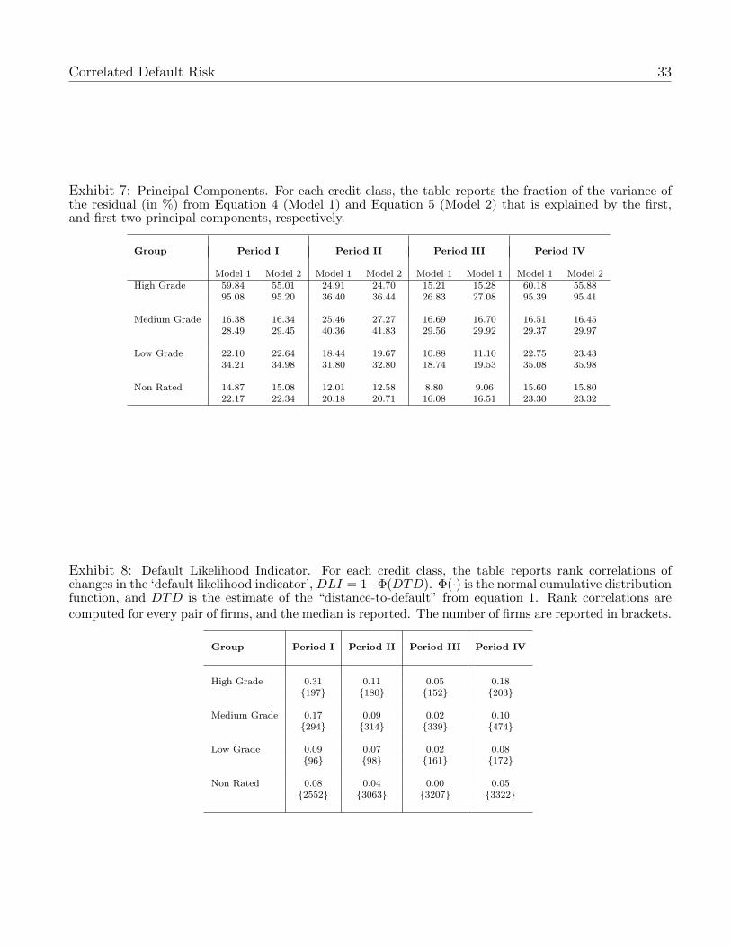
Correlated Default Risk 33
Exhibit 7: Principal Components. For each credit class, the table reports the fraction of the variance ofthe residual (in %) from Equation 4 (Model 1) and Equation 5 (Model 2) that is explained by the first,and first two principal components, respectively.
Group Period I Period II Period III Period IV
Model 1 Model 2 Model 1 Model 2 Model 1 Model 1 Model 1 Model 2High Grade 59.84 55.01 24.91 24.70 15.21 15.28 60.18 55.88
95.08 95.20 36.40 36.44 26.83 27.08 95.39 95.41
Medium Grade 16.38 16.34 25.46 27.27 16.69 16.70 16.51 16.4528.49 29.45 40.36 41.83 29.56 29.92 29.37 29.97
Low Grade 22.10 22.64 18.44 19.67 10.88 11.10 22.75 23.4334.21 34.98 31.80 32.80 18.74 19.53 35.08 35.98
Non Rated 14.87 15.08 12.01 12.58 8.80 9.06 15.60 15.8022.17 22.34 20.18 20.71 16.08 16.51 23.30 23.32
Exhibit 8: Default Likelihood Indicator. For each credit class, the table reports rank correlations ofchanges in the ‘default likelihood indicator’, DLI = 1−Φ(DTD). Φ(·) is the normal cumulative distributionfunction, and DTD is the estimate of the “distance-to-default” from equation 1. Rank correlations arecomputed for every pair of firms, and the median is reported. The number of firms are reported in brackets.
Group Period I Period II Period III Period IV
High Grade 0.31 0.11 0.05 0.18197 180 152 203
Medium Grade 0.17 0.09 0.02 0.10294 314 339 474
Low Grade 0.09 0.07 0.02 0.0896 98 161 172
Non Rated 0.08 0.04 0.00 0.052552 3063 3207 3322

Correlated Default Risk 34
Exhibit 9: Estimation of the Regime Switching model. The table reports estimates from a two-regimemodel for default probabilities. Panel A is for the case of a constant transition matrix, and Panel B forthe case where transition probabilities vary with the short rates. Panel C presents the results when thestate variable is set to average firm return volatility.
Panel A Panel B Panel CConstant Transition r Dependent MKTV OL Dependent
Probabilities Probabilities Probabilities
Parameters Estimates t-stats Estimates t-stats Estimates t-stats
β1 0.78 17.37 0.78 17.21 0.78 18.12β2 0.92 57.48 0.92 51.94 0.92 58.10θ1 1.77% 18.43 1.76% 17.03 1.77% 19.12θ2 0.74% 15.61 0.74% 16.33 0.74% 15.77v1 0.07% 6.57 0.07% 7.61 0.07% 7.56v2 0.04% 15.28 0.04% 16.47 0.04% 15.95a1 1.96 3.39 3.46 0.47 1.41 0.30a2 3.45 6.59 5.14 2.56 7.65 2.28b1 -0.26 -0.39 2.32 0.17b2 -0.29 -0.91 -14.21 -1.31

Correlated Default Risk 35
Dec84 Sep87 Jun90 Mar93 Dec95 Sep98 May010
0.1
0.2
0.3
0.4
0.5
0.6
0.7
0.8
0.9
1
Date
Mea
n of
Def
ault
Inte
nsity
Exhibit 10: Time series of regime probabilities. This figure presents the time series plot of probability ofbeing in the high default intensity regime. The probability of being in the low intensity regime is one minusthe high intensity probabilities, since there are only two regimes in the estimated model. The transitionprobabilities are generated from the model where they are a function of the short rate. The results withconstant transition probabilities or when transition probabilities are a function of volatility are very similar.
Exhibit 11: Regime Dependent Parameters within each Rating Category.For each rating category, i, the table reports the maximum likelihood estimates of the model,
λki (t) = λk
i (t− 1) + (1− βki )[θk
i − λki (t− 1)] + vk
i εi(t), k ∈ 1, 2.
across two regimes. The regimes are based on the estimation in Panel A of Exhibit 9. The t-statistics arereported in parenthesis.
Rating ParametersClass β1
i β2i θ1
i θ2i v1
i v2i
(%) (%) (%) (%)
High 0.97 0.99 0.25 0.11 0.03 0.01(82.00) (49.32) (5.67) (3.77) (7.18) (14.80)
Medium 0.86 0.98 1.48 0.41 0.09 0.05(18.64) (49.37) (9.00) (2.54) (9.37) (17.34)
Low 0.85 0.96 4.81 2.38 0.12 0.12(8.92) (7.77) (8.93) (7.77) (8.21) (16.07)

Correlated Default Risk 36
Exhibit 12: Statistical differences in covariance matrices. This table presents the chi-square statistics forthe differences in covariance matrices in the high and low default regimes. The test was performed on arandomly chosen group of 30 firms from each rating class. The sample is limited to 30 firms as the numberof months in the shorter regime - regime 1 - are thirty. Similar results are obtained for alternative samples.
Rating Class Test-Statistics Degrees of Freedom p-value
High Grade 985.69 465 0.00
Medium Grade 657.65 465 0.00
Low Grade 904.75 465 0.00
Exhibit 13: Probabilities of exactly n defaults from m = 10 bonds. The two tableaus below showthe parameters used and the probabilities of n defaults.
Panel A: Input parametersRating class High default regime Low default regime
(θi%) (v∗i ) Corr (θi%) (v∗i ) CorrHigh 0.25 0.1225 0.38 0.11 0.0707 0.01
Medium 1.48 0.1701 0.25 0.41 0.2500 0.02Low 4.81 0.2191 0.17 2.38 0.4243 0.02
Panel B: Probabilities of n defaultsHigh Default Regime Low Default Regime
Rating Rating Rating Rating Rating RatingNo. Defaults High Medium Low High Medium Low
n p(n) p(n) p(n) p(n) p(n) p(n)0 0.975327 0.862451 0.618184 0.989063 0.959859 0.7882741 0.024387 0.128565 0.304590 0.010883 0.039405 0.1897862 0.000284 0.008632 0.067539 0.000054 0.000728 0.0205623 0.000002 0.000344 0.008875 0.000000 0.000008 0.0013204 0.000000 0.000008 0.000765 0.000000 0.000000 0.000056≥ 5 0.000000 0.000001 0.000047 0.000000 0.000000 0.000002

Correlated Default Risk 37
High Default RegimeProbability of n defaults, p(n)
m = 100
-0.1
0
0.1
0.2
0.3
0.4
0.5
0.6
0.7
0.8
0.9
0 1 2 3 4 5 6 7 8 9 10 11 12 13 14 15 16 17 18 19 20
No of Defaults (n)
PD
F
High Rating
Medium Rating
Low Rating
Low Default RegimeProbability of n defaults, p(n)
m = 100
-0.1
0
0.1
0.2
0.3
0.4
0.5
0.6
0.7
0.8
0.9
1
0 1 2 3 4 5 6 7 8 9 10 11 12 13 14 15 16 17 18 19 20
No of Defaults (n)
PD
F
High Rating
Medium Rating
Low Rating
Exhibit 14: Plots of the probability density functions of the number of defaults n out of m bondsfor the high and low default risk regimes. In this illustration m = 100.

Correlated Default Risk 38
High & Low Risk Regimes
-0.15
-0.1
-0.05
0
0.05
0.1
0 2 4 6 8 10 12 14 16 18 20 22 24 26 28 30
Number of Defaults
Dif
fere
nce i
n P
DFs
High
Medium
Low
Exhibit 15: Difference in the probability p(n) of the number of defaults n, across high and low default riskregimes. The plots below are for each rating class (High, Medium and Low). They depict the difference inthe PDF over the number of defaults, obtained by subtracting the low regime PDF from the high regimeone. The figure shows that the tails of the distribution are fatter for the high risk regime, as would beexpected.
Probability of n defaults in theLow Rating in High vs Low Default Risk Regimes
0
0.2
0.4
0.6
0.8
1
1.2
0 2 4 6 810
12
14
16
18
20
22
24
26
28
30
No of Defaults (N=106)
Cu
mu
lati
ve P
rob
ab
ilit
y
High Default Regime
Low Default Regime
Exhibit 16: Difference in the cumulative probability of the number of defaults n, across high and lowcorrelation regimes for the low rating class. The total number of firms in this class was 106. The greenvertical line represents the cut off for 10% of the total number of firms.