correlation pursuit:forward stepwise variable selection ...junliu/techrept/12folder/cop2012.pdf ·...

© 2012 Royal Statistical Society 1369–7412/12/74000

J. R. Statist. Soc. B (2012)74, Part 4, pp.

Correlation pursuit: forward stepwise variableselection for index models

Wenxuan Zhong,

University of Illinois at Urbana–Champaign, Champaign, USA

Tingting Zhang,

University of Virginia, Charlottesville, USA

Yu Zhu

Purdue University, West Lafayette, USA

and Jun S. Liu

Harvard University, Cambridge, USA

[Received February 2010. Final revision November 2011]

Summary. A stepwise procedure, correlation pursuit (COP), is developed for variable selectionunder the sufficient dimension reduction framework, in which the response variable Y is influ-enced by the predictors X1, X2,. . . ,Xp through an unknown function of a few linear combinationsof them. Unlike linear stepwise regression, COP does not impose a special form of relationship(such as linear) between the response variable and the predictor variables.The COP procedureselects variables that attain the maximum correlation between the transformed response andthe linear combination of the variables. Various asymptotic properties of the COP procedureare established and, in particular, its variable selection performance under a diverging numberof predictors and sample size is investigated. The excellent empirical performance of the COPprocedure in comparison with existing methods is demonstrated by both extensive simulationstudies and a real example in functional genomics.

Keywords: Dimension reduction; Projection pursuit regression; Sliced inverse regression;Stepwise regression; Variable selection

1. Introduction

Advances in science and technology in the past few decades have led to an explosive growth ofhigh dimensional data across a variety of areas such as genetics, molecular biology, cognitivesciences, environmental sciences, astrophysics, finance and Internet commerce. Compared withtheir dimensionalities, a large amount of data sets generated from these areas have relativelysmall sample sizes. Variable (or feature) selection and dimension reduction are more than oftenkey steps in analysing these data. Much progress has been made in the past few decades onvariable selection for linear models (see Shao (1998) and Fan and Lv (2010) for a review). Inrecent years, shrinkage-based procedures for simultaneously estimating regression coefficientsand selecting predictors have been particularly attractive to researchers, and many promising

Address for correspondence: Wenxuan Zhong, Department of Statistics, University of Illinois at Urbana–Cham-paign, 725 South Wright Street, Champaign, IL 61820, USA.E-mail: [email protected]

2 W. Zhong, T. Zhang, Y. Zhu and J. S. Liu

algorithms such as the lasso (Tibshirani, 1996; Zou, 2006; Friedman, 2007), LARS (Efronet al., 2004) and smoothly clipped absolute deviation (SCAD) (Fan and Li, 2001) have beeninvented.

Let Y ∈ R be a univariate response variable and X = .X1, X2, . . . , Xp/′ ∈ Rp a vector of pcontinuous predictor variables. Throughout this paper, we consider the following sufficientdimension reduction (SDR) model framework as pioneered by Li (1991) and Cook (1994).Let β1, β2, . . . , βK be p-dimensional vectors with βi = .β1i, β2i, . . . , βpi/

′ for 1� i�K. The SDRmodel assumes that Y and X are mutually independent conditional on β′

1X, β′2X, . . . , β′

KX, i.e.

Y⊥X|B′X, .1/

where ‘⊥’ means ‘independent of’ and B = .β1, β2, . . . , βK/. Expression (1) implies that all theinformation X contains about Y is contained in the K projections β′

1X, . . . , β′KX. A predictor

variable Xj (1� j �p) is said to be relevant if there is at least one i (1� i�K) such that βji �=0.Let L be the number of relevant predictor variables. When there are a large number of predic-tors (i.e. p is large), it is usually safe to impose the sparsity assumption, which states that onlya small subset of the predictors influences Y and the others are irrelevant. In the SDR model,this assumption means that both K and L are small relative to p.

In his seminal paper on dimension reduction, Li (1991) proposed a seemingly different modelof the form

Y =f.β′1X, β′

2X, . . . , β′KX, "/, .2/

where f is an unknown .K +1/-variate link function and " is a stochastic error independent ofX. It has been shown that the two models (1) and (2) are in fact equivalent (Zeng and Zhu, 2010).We henceforth always refer to β1, β2, . . . , βK as the SDR directions and the space spanned bythese directions as an SDR subspace. In general, SDR subspaces are not unique. To resolve thisambiguity, Cook (1994) introduced the concept of a central subspace, which is the intersectionof all possible SDR subspaces and is an SDR subspace itself, and showed that the central spaceis well defined and unique under some general conditions. We denote the central subspace byS.B/ and assume its existence throughout this paper.

Various methods have been developed for estimating β1, . . . , βK in the literature on SDR. Oneparticular family of methods utilizes inverse regression, which is to regress X against Y. Thesliced inversion regression (SIR) method that was proposed by Li (1991) is the forerunner of thisfamily of methods. Recognizing that estimation of the SDR directions does not automaticallylead to variable selection, Cook (2004) derived various χ2-tests for assessing the contributionof predictor variables to the SDR directions. On the basis of these tests, Li et al. (2005) pro-posed a backward subset selection method for selecting significant predictors. Following therecent trend of using the L1- or L2-penalty for variable selection, Zhong et al. (2005) proposedto regularize the sample covariance matrix of the predictor variables in SIR and developed aprocedure called regularized SIR for variable selection. Li (2007) proposed sparse SIR (SSIR)to obtain shrinkage estimates of the SDR directions. Bondell and Li (2009) further adopted thenon-negative garrotte method for estimating the SDR directions and showed that the resultingmethod is consistent in variable selection.

The majority of the aforementioned methods take a two-step approach to variable selectionunder the SDR model. The first step is to perform dimension reduction, i.e. to estimate theSDR directions; and the second step is to select the relevant variables by using statistical testingor shrinkage methods. Because these methods need to estimate the covariance and conditionalcovariance matrices of X , both of which are of dimensions p×p, the effectiveness and robust-ness of the two-step approach are questionable when p is large relative to n. Zhu et al. (2006) have

Correlation Pursuit 3

shown that the accuracy of estimation of SDR directions deteriorates as p increases. In otherwords, the more irrelevant variables there are, the more likely a method fails to estimate theSDR directions accurately, and the less likely the method identifies the true relevant predictorvariables.

In this paper, we propose correlation pursuit (COP), which is a stepwise procedure for simul-taneous dimension reduction and variable selection under the SDR model. Similar to projectionpursuit (Friedman and Tukey, 1974; Huber, 1985), COP defines a projection function to mea-sure the correlation between the transformed response and the projections of X and pursues asubset of explanatory variables that maximize the projection function. It starts with a randomlyselected subset and iterates between finding an explanatory variable (predictor) that significantlyimproves the current projection function to add to the subset and finding an insignificant pre-dictor to remove from the subset. During each iteration step, COP needs only to consider thepredictors that are currently in the subset and one more predictor outside the subset. Therefore,COP can avoid the estimation and inversion of p × p covariance and conditional covariancematrices of X and mitigate the curse of dimensionality. Furthermore, COP performs dimensionreduction and variable selection simultaneously. Therefore, dimension reduction and variableselection can be mutually enhanced. Our theoretical investigations as well as simulation stud-ies show that COP is a promising tool for dimension reduction and variable selection in highdimensional data analysis.

The rest of the paper is organized as follows. In Section 2, we give a brief introduction toSIR, following a correlation interpretation of SIR that was provided by Chen and Li (1998).This interpretation was also used in Fung et al. (2002) and Zhou and He (2008) for dimensionreduction via canonical correlation. In the same section, we describe the COP procedure andderive various test statistics that are used by the procedure. The asymptotic behaviour of theCOP procedure is discussed in Section 3. Several implementation issues of the procedure arediscussed in Section 4. Simulation and real data examples are reported in Sections 5 and 6respectively. Additional remarks in Section 7 conclude the paper. An abbreviated version of theproofs of the theorems is provided in Appendix A.

2. Correlation pursuit for variable selection

2.1. Profile correlation and sliced inverse regressionLet η be an arbitrary direction in Rp. We define the profile correlation between Y and η′X, whichis denoted by P.η/, as

P.η/=maxT

[corr{T.Y/, η′X}], .3/

where the maximization is taken over all possible transformations of Y including non-monotonetransformations. The profile correlation P.η/ reflects the largest possible correlation betweena transformed response T.Y/ and the projection η′X. Let η1 be the direction that maximizesP.η/ subject to η′Ση = 1, i.e. η1 = arg maxη′Ση=1{P.η/}. We refer to η1 as the first principaldirection for the profile correlation between Y and X and call P.η1/ the first profile correla-tion. Direction η1, or its projection η′

1X, may not entirely characterize the dependence betweenY and X. Using P.η/ as the projection function again, we can look for a second direction,which is denoted by η2, which is uncorrelated with η′

1X, i.e. η′2Ση1 = 0, and maximizes P.η/,

i.e. η2 = argmaxη:η′Ση1=0{P.η/}: We refer to η2 as the second principal direction and P.η2/ asthe second profile correlation. This procedure can be continued until no more directions canbe found that are orthogonal to the directions obtained and have a non-zero profile correla-tion with Y. Suppose that K principal directions exist between Y and X , which are η1, η2, . . . ,


and ηK, with the corresponding profile correlations P.η1/ � P.η2/ � . . . P.ηK/ > 0. We need toimpose the following condition to establish the connection between the principal directions andthe SDR directions under the SDR model.

Condition 1 (linearity condition). For any η in Rp, E.η′X|B′X/ is linear in B′X, where B isas defined in equation (1).

Proposition 1. Under the SDR model and the linearity condition, the principal directionsη1, η2, . . . , ηK are in the central space S.B/.

To make this paper self-sufficient, we have included the proof of proposition 1 in AppendixA. Based on the proposition, the principal directions are indeed SDR directions. In general,K < K. When the link function f is symmetric along a direction, using correlation alone mayfail to recover this direction. For example, if Y =X2

1 + ", the profile correlation between Y andX1 will always be 0. To exclude this possibility, we follow the convention in the SDR literatureto impose the following condition.

Condition 2 (coverage condition). The number of principal directions of profile correlation isequal to the dimensionality of the central subspace, i.e. K =K.

Under both the linearity and the coverage conditions, the principal directions η1, η2, . . . , ηK

form a special basis of the central subspace S.B/, i.e. S.B/ = span.η1, η2, . . . , ηK/. This basisis uniquely defined and is the estimation target of SIR. In the rest of the paper, for ease ofdiscussion, we use β1, β2, . . . , βk and η1, η2, . . . , ηK, interchangeably.

Chen and Li (1998) showed that, at the population level, there is an explicit solution for theprincipal directions. In the proof of their theorem 3.1, Chen and Li (1998) derived that

P2.η/= η′ var{E.X|Y/}η

η′Ση≡ η′Mη

η′Ση, .4/

where M=Δ var{E.X|Y/} is the covariance matrix of the expectation of X given Y. Furthermore,the principal directions of profile correlation are the solutions of the eigenvalue decompositionproblem

Mvi =λiΣvi, v′iΣvi =1, for i=1, 2, . . . , K; .5/

λ1 �λ2 �. . . �λK > 0: .6/

The principal directions η1, η2, . . . , and ηK are the first K eigenvectors of Σ−1M, and theircorresponding eigenvalues are exactly the squared profile correlations, i.e. P2.ηi/ =λi for i =1, 2, . . . , K.

Given independent observations {.xi, yi/}i=1,:::,n of .X, Y/, where xi = .xi1, . . . , xip/′, Σ canbe estimated by the sample covariance matrix,

Σ=

n∑i=1

.xi − x/.xi − x/′

n−1, .7/

where x is the sample mean of {xi}. Li (1991) proposed the following SIR procedure to estim-ate M. First, the range of {yi}n

i=1 is divided into H disjoint intervals, which are denoted asS1, . . . , SH . For h = 1, . . . , H , the mean vector xh = n−1

h Σyi∈Shxi is calculated, where nh is the

number of yis in Sh. Then, M is estimated by


M =

H∑h=1

nh.xh − x/. xh − x/′

n, .8/

and the matrix Σ−1M is estimated by Σ−1

M. The first K eigenvectors of Σ−1

M, which aredenoted by η1, η2, . . . , ηK, are used to estimate the first K eigenvectors of Σ−1M or, equivalently,the principal directions η1, η2, . . . , ηK respectively. The first K eigenvalues of Σ

−1M, which are

denoted by λ1, λ2, . . . , λK, are used to estimate the eigenvalues of Σ−1M or, equivalently, thesquared profile correlations λ1, λ2, . . . , λK respectively.

2.2. Correlation pursuitThe SIR method needs to estimate the two p×p covariance matrices Σ and M , and to obtainthe eigenvalue decomposition of Σ

−1M. When a large number of irrelevant variables are present

and the sample size n is relatively small, Σ and M become unstable, which leads to very inaccu-rate estimates of principal directions η1, η2, . . . , ηK (Zhu et al., 2006). As a consequence, thoseshrinkage-based variable selection methods that rely on η1, η2, . . . , ηK often perform poorly forthe SDR model when p is large. We here propose a stepwise SIR-based procedure for simulta-neous dimension reduction (i.e. estimating the principal directions) and variable selection (i.e.identifying true predictors). Our procedure starts with a collection of randomly selected predic-tors and iterates between an addition step, which selects and adds a predictor to the collection,and a deletion step, which selects and deletes a predictor from the collection. The procedureterminates when no new addition or deletion occurs.

2.2.1. Addition stepLet A denote the collection of the indices of the selected predictors and XA the collection ofthe selected variables. Applying SIR to the data involving only the predictors in XA, we obtainthe estimated squared profile correlations λA

1 , λA2 , . . . , λA

K . Superscript A indicates that the es-timated squared profile correlations depend on the current subset of selected predictors. Let Xt

be an arbitrary predictor outside A and A+ t =A∪{t}. Applying SIR to the data involving thepredictors in A+ t, we obtain the estimated squared profile correlations λA+t

1 , λA+t2 , . . . , λA+t

K .Because A⊂A+ t, it is easy to see that λA

1 � λA+t1 . The difference λA+t

1 − λA1 reflects the amount

of improvement in the first profile correlation due to the incorporation of Xt . We standardizethis difference and use the resulting test statistic

COPA+t1 = n.λ

A+t

1 − λA1 /

1− λA+t

1

, .9/

to assess the significance of adding Xt to A in improving the first profile correlation. Similarly,the contributions of adding Xt to the other profile correlations can be assessed by

COPA+ti = n.λ

A+t

i − λAi /

1− λA+t

i

, .10/

for 2 � i � K. The overall contribution of adding Xt to the improvement in all the K profilecorrelations can be assessed by combining the statistics COPA+t

i into one single test statistic

COPA+t1:K =

K∑i=1

COPA+ti : .11/


We further define that

COPA1:K =maxt∈Ac .COPA+t

1:K /: .12/

Let Xt be a predictor that attains COPA1:K, i.e. COP

A1:K = COPA+t

1:K , and let ce be a prespecifiedthreshold (details about its choice are deferred to the next two sections). Then, if COP1:K

A> ce,

we add t to A; otherwise, we do not add any variable.

2.2.2. Deletion stepLet Xt be an arbitrary predictor in A and define A− t =A−{t}. Let λ

A−t

1 , λA−t

2 , . . . , λA−t

K bethe estimated squared profile correlations based on the data involving the predictors in A− t

only. The effect of deleting Xt from A on the ith squared profile correlation can be measuredby

COPA−ti = n.λ

Ai − λ

A−t

i /

1− λAi

, .13/

for 1� i�K. The overall effect of deleting Xt is measured by

COPA−t1:K =

K∑i=1

COPA−ti , .14/

and the least effect from deleting one predictor from A is then defined to be

COPA1:K =mint∈A.COPA−t

1:K /: .15/

Let Xt be a predictor that achieves COPA1:K, and let cd be a prespecified threshold for deletion.

If COPA1:K <cd, we delete Xt from A; otherwise, no deletion happens.

The asymptotic distributions of the proposed statistics and the selection of the thresholds willbe discussed in the next two sections. Because the procedure described aims to find predictorsthat can most significantly improve the profile correlations between Y and X , we call it the COPprocedure. Below we summarize the COP algorithm.

Step 1: set the number of principal directions K and the threshold values ce and cd.Step 2: randomly select K +1 variables as the initial collection of selected variables A.Step 3: iterate until no more addition or deletion of predictors can be performed; in theaddition step,

(a) find t such that COPA+t1:K =COP

A1:K and

(b) if COPA1:K >ce, add t to A, i.e. let A=A+ t;

in the deletion step,

(a) find t such that COPA−t

1:K =COPA1:K and

(b) if COPA1:K <cd, delete t from A, i.e. let A=A− t.

Step 4: output A.

3. Theoretical properties

3.1. Asymptotic distributions of test statistics in correlation pursuitLet us first consider an addition step. We assume that SIR uses a fixed slicing scheme relative tothe number of observations n, i.e. the slices S1, S2, . . . , SH are fixed (defined by the range of the


response variable) but the number of observations in each slice goes to ∞. Let Xt be an arbitrarypredictor in Ac. Under the null hypothesis H0 that all the predictors in Ac are irrelevant, we haveηt1 =ηt2 = . . . =ηtK =0. Recall that the statistics we propose to measure the contributions of Xt

to the K profile correlations are .COPA+t1 , COPA+t

2 , . . . , COPA+tK /′, and to measure the overall

contribution of Xt by COPA+t1:K . To establish the asymptotic distributions of these statistics, we

need to impose a condition on the conditional expectation of Xt given XA.

Condition 3 (regression condition). E.Xt|XA/ is linear in XA.

Theorem 1. Assume that conditions 1 and 2 hold, condition 3 holds for .XA, Xt/ for anyXt ∈XAc , and the squared profile correlations λ1, λ2, . . . , λK are positive and different fromeach other. Then, for any given fixed slicing scheme, under the null hypothesis H0 that all thepredictors in Ac are irrelevant, we have that

.COPA+t1 , COPA+t

2 , . . . , COPA+tK /→ .Z2

1t , Z22t , . . . , Z2

Kt/ .16/

in distribution and

COPA+t1:K →

K∑l=1

Z2lt .17/

in distribution as n → ∞. Here, .Z1t , Z2t , . . . , ZKt/ follows the multivariate normal distri-bution with mean 0 and covariance matrix WKt . The explicit expression of WKt is given inAppendix A.

The asymptotic distributions in theorem 1 can be much simplified if we impose the followingcondition on the variance of the conditional expectation of Xt given XA.

Condition 4 (constant variance condition). E[{Xt −E.Xt|XA/}2|XA] is a constant.

Corollary 1. Assume that conditions 1 and 2 hold, conditions 3 and 4 hold for .XA, Xt/

for Xt ∈XAc and the squared profile correlations λ1, λ2, . . . , λK are positive and different fromeach other. Then, for any given fixed slicing scheme, under the null hypothesis H0 that all thepredictors in Ac are irrelevant, we have that COPA+t

1 , COPA+t2 , . . . , COPA+t

K are asymptoticallyindependent and identically distributed as χ2.1/, and COPA+t

1:K is asymptotically χ2.K/.

Theorem 1 and corollary 1 characterize the asymptotic behaviours of the test statistics for anarbitrary Xt in Ac. In the COP procedure, however, the predictor that attains the maximum valueof COPA+t

1:K among t ∈Ac, which is COPA1:K, is considered a candidate predictor to enter A. Our

next theorem characterizes the joint asymptotic behaviour of {COPA+t1:K }t∈Ac as well as that of

COPA1:K.

The linearity, regression and constant variance conditions together are more general thanthe normality assumption on X because they only need to hold for the basis of the centralsubspace (e.g. B or η1, . . . , ηK) and a given subset of predictors (e.g. A). If we require that theconditions hold for any projection and any given subset of the predictors, however, then it isequivalent to requiring that X follows a multivariate normal distribution. To understand thejoint behaviour of all the COP statistics, in what follows we impose the normality assumptionon X.

Let A = {tj}dj=1 and Ac = {tj}p

j=d+1 denote the collection of currently selected predictorsand its complement respectively. Let ΣA = cov.XA/, ΣAc = cov.XAc /, ΣAAc = cov.XA, XAc /

and ΣAc =ΣAc −ΣAcAΣ−1A ΣAAc . Note that ΣAcA =Σ′

AAc . Let a = .a1, a2, . . . , ap−d/′ be thevector of the diagonal elements of ΣAc . Define DAc =diag.a1, a2, . . . , ap−d/, and define UAc =D

−1=2Ac ΣAc D

−1=2Ac .


Theorem 2. Assume that

(a) X follows a multivariate normal distribution,(b) the coverage condition holds and(c) the squared profile correlations λ1, λ2, . . . , λK are non-zero and different from each other.

Then, for any fixed slicing scheme, under the null hypothesis H0 that all the predictors in Ac

are irrelevant, we have

.COPA+td+11:K , COPA+td+2

1:K , . . . , COPA+tp1:K /

D→(

K∑k=1

z2k,d+1, . . . ,

K∑k=1

z2k,p

), .18/

and

COPA1:K

D→maxt∈Ac

(K∑

k=1z2

k,t

).19/

as n→∞. Here zk = .zk,d+1, . . . , zk,p/ for k =1, . . . , K are mutually independent and each zk

follows a multivariate normal distribution with mean 0 and covariance matrix UAc :

We now consider deletion steps of the COP procedure. We let A denote the current collec-tion of selected predictors before a deletion step, and we let Xt be an arbitrary predictor in A.Note that COPA−t

k =COPA+tk , where A=A− t for 1�k �K. Therefore, results similar to those

stated in theorem 1 and corollary 1 can be obtained for .COPA−t1 , COPA−t

2 , . . . , COPA−tK / and

COPA−t1:K after some modifications described below. First, our current ‘null hypothesis’, which

is denoted as H0t , is that Xt and the predictors in Ac are irrelevant. Second, the regression andconstant variance conditions need to be imposed on the conditional expectation of Xt given XAinstead. The asymptotic distribution of COPA

1:K, however, turns out to be fairly complicated ifnot entirely elusive, because there is not a common null hypothesis for all Xt ∈A. In what follows,we shall establish two strong results that have implications for properly selecting the thresholdsce and cd, as well as for the consistency of the COP procedure in selecting true predictors.

3.2. Selection consistency of correlation pursuitLet T be the collection of the true predictors under the SDR model. The principal profilecorrelation directions are η1, η2, . . . , ηK, which form a basis of the central subspace. Assumethat S1, . . . , SH is a fixed slicing scheme that is used by SIR. Let ph = P.y ∈ Sh/, vK = .η′

1X −E.η′

1X/, . . . , η′KX−E.η′

KX//′ and

MH ,K =H∑

h=1phLh,KL′

h,K, .20/

where Lh,K = E.vK|Y ∈ Sh/. A few more conditions are needed for the results that we state inthe next two theorems.

Condition 5. X follows a multivariate normal distribution with covariance matrix Σ such thatτmin �λmin.Σp/�λmax.Σp/�τmax, where τmin and τmax are two positive constants, and λmin.·/and λmax.·/ are the minimum and maximum eigenvalues of a matrix respectively.

Condition 6. There is a constant ωH > 0 such that λmin.MH ,K/>ωH:

Condition 7. There are constants σ20 and υ > 0 such that, for any slice Sh and any two pre-

dictors Xi and Xj, var.Xj|Y ∈ Sh/ � σ20 and var.XiXj|y ∈ Sh/ � σ2

0 for all i, j = 1, . . . , p, andh=1, . . . , H: In addition,

E.|Xj|l|Y ∈Sh/� l!2

var.Xj|Y ∈Sh/υl−2


and

E.|XiXj|l|Y ∈Sh/� l!2

var.XiXj |Y ∈Sh/υl−2, for l�2:

Condition 8.Let ηj = .ηj1, ηj2, . . . , ηjK/′ in which ηjk is the coefficient of Xj in the kth principalcorrelation direction ηk. There is a positive constant >0 and a non-negative constant ξ0, suchthat ‖ηj‖2 >n−ξ0 for j ∈T , where ‖·‖ denotes the standard L2-norm.

Condition 9. limn→∞.p/=∞ and p=o.n�0/ with �0 �0 and 2�0 +2ξ0 < 1:

Condition 5 ensures that the variances of the predictors are on a comparable scale and thatthey are not strongly correlated. Condition 6 assumes a lower bound for the eigenvalues ofMH ,K, which is slightly stronger than the coverage condition that ensures SIR to recover all theSDR directions. Condition 7 imposes conditions on the moments of the conditional expecta-tions of X given Y ∈Sh so that the Bernstein inequalities hold for the conditional sample means.Condition 8 assumes that the coefficients of any true predictors do not decrease to 0 too fast asboth n and p increase; otherwise, such predictors will not be identifiable asymptotically. Con-dition 9 allows p to increase as n increases, but their rates are constrained. Similar conditionshave been used by others for establishing variable selection results for stepwise procedures inlinear regression (Wang, 2009; Fan and Lv, 2008).

Theorem 3. Let A be the set of currently selected predictors and let T be the set of truepredictors. Let ϑ=ωHτ2

min=2τmax: Assume that conditions 5–9 hold. Then, we have

P{ minA:Ac∩T �=∅

maxt∈Ac∩T

.COPA+t1:K /�ϑn1−ξ0}→1, .21/

for any fixed slicing scheme as n→∞.

The probability statement (21) is not just about one given collection of predictors. It con-siders all the possible collections that do not include all the true predictors yet, i.e. {A : Ac ∩T �= ∅}. In other words, it considers all the possible scenarios where the null hypothesis H0is not true. Further note that maxt∈Ac∩T .COPA+t

1:K / �= COPA1:K. Because maxt∈Ac .COPA+t

1:K / �maxt∈Ac∩T .COPA+t

1:K /, from equation (21), we have

P{ minA:Ac∩T �=∅

.COPA1:K/�ϑn1−ξ0}→1: .22/

This result implies that by setting ce to ϑn1−ξ0 or smaller, if the COP procedure has not collectedall the true predictors yet, then with probability going to 1 (as n→∞) it will continue to selecta predictor to the current collection. Thus, the addition step of COP will not stop until all thetrue predictors have been selected. Another way to interpret expression (22) is that the selectionpower of the COP procedure converges to 1 asymptotically.

Theorem 4. Assume that conditions 5–9 hold. Then we have

P{ maxA:Ac∩T =∅

maxt∈Ac

.COPA+t1:K /<Cn�}→1, .23/

for �> 12 +�0, and any positive constant C, under any fixed slicing scheme with n→∞.

Theorem 4 has two implications. The first regards the addition step of COP. Once all the truepredictors have been selected, i.e. Ac ∩T =∅, the probability that it will select a false predic-tor from Ac converges to 0. The second implication concerns the deletion step. Consider onecollection of selected predictors A and assume that A contains all the true predictors and also


some irrelevant ones, i.e. A⊃T . Clearly,

COPA1:K � min

t∈A−T.COPA−t

1:K /� maxA:Ac∩T =∅

maxt∈Ac

(K∑

k=1COPA+t

k

): .24/

Therefore,

P.COPA1:K <Cn�/→1: .25/

In other words, with probability going to 1, the COP procedure will delete an irrelevant predictorfrom the current collection.

One possible choice of the thresholds is χ2e = ϑn1−ξ0 and χ2

d = ϑn1−ξ0=2. From theorem 3,asymptotically, the COP algorithm will not stop selecting variables until all the true predictorshave been included. Moreover, once all the true predictors have been included, according totheorem 4, all the redundant variables will be removed from the selected variables.

4. Implementation issues

When implementing the COP algorithm, we need to specify the number of profile correlationdirections K , the thresholds for the addition and deletion steps ce and cd, and the slicing scheme,particularly the number of slices H. A proper specification of these tuning parameters is criticalfor the success of the COP algorithm.

4.1. Slicing schemes and the choice of HLi (1991) suggested that, in terms of estimation, the performance of SIR is robust to the numberof slices in general. The COP algorithm uses SIR to derive test statistics for selecting variables.It is of interest to understand the effect of a slicing scheme on the testing procedures involved.Again, we consider an addition step in the COP procedure. Let A be the current collection ofselected predictors. Let Xt be an arbitrary predictor in Ac.

Theorem 5. Assume that X follows a multivariate normal distribution. Then, for any givenfixed slicing scheme, we have

P

(COPA

1:K

n�CH ,A+t

)→1, as n→∞, .26/

where

CH ,A+t = .ηt,A/′MH ,Kηt,A=σ2t,A, .27/

σ2t,A =var.Xt|XA/, ηt,A = cov.Xt , vK|XA/ and MH ,K is defined in equation (20).

The difference between theorem 1 and theorem 5 is that the latter does not assume that Xt

is an irrelevant predictor. When Xt is indeed a true predictor, then ηt is not a zero vector andmaxt∈Ac∩T .CH ,A+t/ is greater than 0. The larger CH ,A+t is, the more likely Xt will be addedto A. The next result shows that a finer slicing scheme leads to higher power for the additionstep by COP. For any two different slicing schemes S = .S1, . . . , SH1/ and S′ = .S′

1, . . . , S′H2

/, wesay that S′ is a refinement of S, which is denoted by S′ �S, if, for any S′

h′ ∈S′, there is an Sh ∈S

such that S′h′ ⊆Sh.


Proposition 2. Suppose that S and S′ are two slicing schemes such that S′ �S. Then, for anyη ∈RK, we have

η′MH2,Kη �η′MH1,Kη, .28/

where MH2,K and MH1,K are defined as in equation (20) under the slicing schemes S′ and Srespectively.

Proposition 2 implies that the constant CH ,A in theorem 5 becomes larger when a finer slicingscheme is used. This further suggests that the power of the COP procedure in selecting truepredictors tends to increase if a slicing scheme uses a larger number of slices. However, whena slicing scheme uses a larger number of slices, the number of observations in each slice willdecrease, which makes the estimate of E.X|y∈Sh/ less accurate and further makes the estimatesof M = cov{E.X|Y/} and its eigenvalues λ1, . . . , λK less stable. The success of the COP proce-dure hinges on a good balance between the number of slices and the number of observationsin each slice. We observed from intensive simulation studies that, with a reasonable number ofobservations in each slice (say 20 or more), a large number of slices is preferred.

4.2. Choice of ce and cdSection 3 has characterized the asymptotic distributions or behaviours of the test statistics thatare involved in the COP procedure. In theory, these results (theorems 4 and 5) can be used forchoosing the thresholds ce and cd. In practice, however, these thresholds should be used withmuch caution because of the following concerns. First, the distributions that were obtained inSection 3 are for a single addition or deletion step and under various assumptions. Second,the distributions are valid only in an asymptotic sense. In what follows, we propose to use across-validation (CV) procedure for selecting ce and cd.

Let {αi}1�i�d be a prespecified grid on a subinterval in .0, 1/ and {χ2αi,K}1�i�d be the collec-

tion of the 100αith percentile of χ2K. For convenience, we consider only the m pairs of ce =χ2

αi,Kand cd =χ2

αi−0:05,K for 1� i�m. Note that cd <ce and that there is only one tuning parameterthat we need to determine. We follow the general fivefold CV scheme to select the best pair ofce and cd. We randomly divide the original data into five equal-sized subsets and then applythe COP procedure to any four subsets to generate the estimation and variable selection results.The remaining subset of the data is used to test the model and to generate a performance mea-surement. The performance measurements are averaged and the result is used as the CV score.We choose the pair of ce and cd that mazimizes the CV score.

We define the performance measure that is used in the CV procedure as follows. Suppose thatA is the collection of selected predictors and η1,A, . . . , ηK,A are the estimates of the principalprofile correlation directions produced by applying the COP procedure to the training data set.We consider the first principal profile correlation direction first. Recall that η1,A is the directionthat achieves the maximum correlation of a linear projection of X and the transformed responseY , and the optimal transformation is T1.Y/=E.η′

1,AX|Y/ (theorem 3.1 in Chen and Li (1998)).With η1,A estimated by η1,A by using the training data, we apply LOESS proposed by Cleveland(1979) to fit T1.Y/ using the training data and we denote the fitted transformation as T 1.·/. LetX and Y be the data matrix and the response vector of the testing data set. Then, the squaredprofile correlation between X and Y based on the direction η1,A and transformation T 1.·/ iscomputed as corr2{T 1.Y /, η′

1,AX}. Similarly, the squared profile correlations between X and Y

along η2,A, . . . , ηK,A can be calculated. The overall performance measure is defined to be

PC=K∑

k=1corr2{T k.Y /, η′

k,AX}: .29/


The CV score for any pair .ce, cd/ is defined to be the average PC over the five possible partitionsof the training–test data sets.

4.3. Selection of the number of directions KTo determine K , the number of principal profile correlation directions, we adopt a Bayesianinformation criterion type of criterion proposed by Zhu et al. (2006). For any given K between1 and J , where J � max.n, p/ is a reasonable upper bound chosen by the user, we apply theCOP procedure with K = k. Suppose that the resulting collection of the selected predictors isAk and the cardinality of Ak is pk. Using the data involving only the selected predictors, we canestimate M =cov{E.XAk

|Y/} as before and denote the result as M. Let θ1 � θ2 � . . . � θp be theeigenvalues of M + Ipk

, where Ipkis the pk ×pk identity matrix, and let τ be the number of θis

that are greater than 1. Define

G.k/=− log{L.k/}+ log.n/

2k.2pk −k +1/, .30/

where log{L.k/}=Σpi=min.τ ,k/+1{log.θi/+1− θi}. We choose K =argmin1�k�J{G.k/}. In the

original criterion that was proposed by Zhu et al. (2006), they showed that the criterion pro-duces a consistent estimate of K for fixed pk. Our simulation study shows that the modifiedcriterion leads to the correct specification of K for the COP procedure and can be generallyused in practice.

5. Simulation study

We have performed extensive simulation studies to compare the COP algorithm with a few exist-ing variable selection methods and we shall present three examples in this section. When imple-menting the COP algorithm in these examples, we use the CV procedure and the G informationcriterion that was discussed in the previous section to select the thresholds ce and cd and thedimensionality K respectively. The grid that was used for selecting ce is {χ2

0:90,K, χ20:95,K, χ2

0:99,K,χ2

0:999,K, χ20:9999,K}, and the associated grid for selecting cd is {χ2

0:85,K, χ20:90,K, χ2

0:94,K, χ20:949,K,

χ20:9499,K}. The range that was used for selecting K is from 1 to 4 (i.e. J =4). For SSIR, we used

the grid {0, 0:1, . . . , 0:9, 1}×{0, 0:1, . . . , 0:9, 1} to select the pair of tuning parameters that leadsto its best performance. Both COP and SSIR involve slicing the range of the response variable,for which we use the same scheme to facilitate fair comparison.

5.1. Linear modelsIn this example, we consider the linear model

Y =Xβ +σ", .31/

where X = .X1, X2, . . . , Xp/′ follows a p-variate normal distribution with mean 0 and covari-ances cov.Xi, Xj/ = ρ|i−j| for 1 � i, j � p, and " is independent of X and follows N.0, 1/. Thevariable selection methods that we compare the COP procedure with include the lasso, SCAD(Fan and Li, 2001), MARS and SSIR (Li, 2007). The R packages SIS, lars and mda are used torun SCAD, the lasso and MARS respectively. The tuning parameters that are involved in SCADand the lasso are selected by CV. We use the code that was provided by the original authorsto run SSIR. In this example, we consider two specifications of the linear model given below:scenario 1,

p=8, β = .3, 1:5, 2, 0, 0, 0, 0, 0/′, σ =3, ρ=0:5;

scenario 2,


p=1000, β = .3, 1:5, 1, 1, 2, 1, 0:9, 1, 1, 1, 0, . . . , 0/′, σ =1, ρ=0:5:

Under scenario 1, model (31) involves three true predictors and five irrelevant variables, andwas originally used in Tibshirani (1996) and Fan and Li (2001) to demonstrate the empir-ical performances of the lasso and SCAD. We randomly generated 100 data sets from sce-nario 1, each with 40 data points (i.e. n = 40), and applied the aforementioned methods tothe data sets. Two quantities were used to measure the variable selection performance of eachmethod, which are the average number of irrelevant predictors falsely selected as true pre-dictors (which is denoted by FP) and the average number of true predictors falsely excludedas irrelevant predictors (which is denoted by FN). Under scenario 1.1, the FPs and FNsrange from 0 to 5 and from 0 to 3 respectively, with small values indicating good perfor-mances in variable selection. The FP- and FN-values of the methods tested are reported inTable 1.

Under scenario 2, model (31) involves 10 true predictors and 990 irrelevant predictors and isclearly more challenging than scenario 1. We randomly generated 100 data sets each with 200data points (i.e. n = 200) from scenario 2. In each data set, n < p. Similarly to scenario 1, weapplied the methods mentioned above to the data sets and report the FP- and FN-values ofthese methods in Table 1. The tuning parameters in all these methods are determined by CV.

From the left-hand panel of Table 1, under scenario 1, SSIR has the lowest FP-value (FP=0:19), i.e. the average number of irrelevant variables selected by SSIR is 0.19, and COP has thethird lowest FP-values (0.71). The other methods tend to have more false positive results thanSSIR and COP. In terms of FNs, the order of the methods ranked from the lowest to the highestis MARS, SCAD, the lasso, COP and SSIR. The relative sub-par performance of COP andSSIR is because these two methods are developed for variable selection under models that aremore general than the linear model.

From the right-hand panel of Table 1, under scenario 2, COP has the lowest FP-value (FP=2:28). In terms of FN, the lasso and MARS have the lowest value with COP following modestlybehind. Compared with MARS, COP has a much lower FP-value and a slightly higher FN-value. SSIR breaks down under scenario 2 because the variance–covariance matrix of X is nolonger invertible. In terms of both FP and FN, COP outperformed SCAD under this scenario.One explanation for this comparison result is that SCAD involves non-convex optimization andcan be unstable in implementation.

Table 1. Performance comparison under linear models†

Method Results for p=8, n=40, Results for p=1000, n=200,σ =3, ρ=0.5 σ =1, ρ=0.5

FP (0, 5) FN (0, 3) FP (0, 990) FN (0, 10)

LASSO 0.77 (0.093) 0.16 (0.037) 8.87 (0.586) 0.00 (0.000)SCAD 0.67 (0.094) 0.10 (0.030) 6.05 (0.926) 1.16 (0.150)MARS 4.00 (0.059) 0.04 (0.020) 30.64 (0.165) 0.00 (0.000)SSIR 0.19 (0.051) 0.96 (0.068) ‡ ‡COP 0.71 (0.080) 0.56 (0.066) 2.28 (0.203) 0.75 (0.095)

†FP is the average number of irrelevant variables that are falsely selectedby the method, and FN is the average number of true variables that arefalsely excluded by the method; the numbers in parentheses are the stan-dard error of FP or FN.‡The algorithm broke down.


5.2. Non-linear multiple-index modelsIn this example, we consider the multiple-index model

Y = X1 +X2 + . . .+Xd

0:5+ .1:5+X2 +X3 +X4/2 +σ", .32/

where X1, . . . , Xp are independent identically distributed N.0, 1/ random variables, " is N.0, 1/

and independent of X , and d and σ are parameters that need to be further specified. This modelwas originally used in Li (1991) for demonstrating the performance of SIR. It is not difficultto see that, given the two projections X1 +X2 + . . .+Xd and X2 +X3 +X4, Y and X are inde-pendent of each other. The dimensionality of the central subspace of model (32) is 2, and thecollection of true predictors is {X1, . . . , Xd}∪{X2, X3, X4}. Because model (32) is non-linear,methods that were designed specifically for linear models such as the lasso and SCAD are clearlyat a disadvantage. Therefore, in this example, we compare the performances of MARS, SSIRand COP only.

By specifying p, d and σ at different values, we have the following three scenarios: scenario 3,

p=30, d =3, σ =0:1;

scenario 4,

p=30, d =3, σ =2;

scenario 5,

p=400, d =8, σ =0:1:

For each scenario, we generated 100 data sets each with 200 observations (i.e. n= 200) andapplied MARS, SSIR and COP to each data set. The resulting FP- and FN-values are reportedin Table 2.

For scenario 3, MARS achieved the lowest FN-value (0.03), but its FP-value was unacceptablyhigh (16.55); SSIR had the lowest FP-values, but its FN-value was the highest among the three.The FP- and FN-values of COP were between the extremes. It appears that the performances ofSSIR and COP are similar under scenario 3. For scenario 4, COP outperformed SSIR in termsof both FP- and FN-values. MARS again achieved the lowest FN-value (0.32) at the expense of

Table 2. Performance comparison under the multiple-index model†

Method Results for σ =0.1, Results for σ =2, Results for σ =0.1,p=30, d =3 p=30, d =3 p=400, d =8

FP (0, 26) FN (0, 4) FP (0, 26) FN (0, 4) FP (0, 292) FN (0, 8)

MARS 16.55 (0.174) 0.03 (0.017) 17.18 (0.186) 0.32 (0.053) ‡ ‡SSIR 0.12 (0.033) 0.91 (0.029) 4.14 (0.288) 1.76 (0.115) ‡ ‡COP 1.88 (0.149) 0.83 (0.038) 3.26 (0.210) 1.71 (0.104) 8.93 (0.576) 0.18 (0.081)

†FP is the average number of irrelevant variables that are falsely selected by the method, and FNis the average number of true variables that are falsely excluded by the method; the numbers inparentheses is the standard error of FP or FN.‡The algorithm broke down.


an unacceptable FP-value (17.18). Scenario 5 is the most challenging among the three scenarios,in which the number of predictors exceeds the number of observations. Both MARS and SSIRbroke down under this scenario. However, COP still demonstrated an excellent performancewith its FP- and FN-values reasonably low.

5.3. Heteroscedastic modelsIn the previous examples, the true predictors affect only the mean response. In this example, weconsider the heteroscedastic model

Y = 0:2"

1:5+p∑

j=1βj,1Xj

, .33/

where X = .X1, X2, . . . , Xp/′ follows a p-variate normal distribution with mean 0 and covari-ances cov.Xi, Xj/ = ρ|i−j| for 1 � i, j � p, " is independent of X and follows N.0, 1/, and βj,1equals 1 for 1 � j � 8 and equals 0 for j � 9. Note that the central subspace is spanned byβ1 = .β1,1, β2,1, . . . , βp,1/′ and the number of true predictors is 8. We further specify ρ and p inequation (33) and consider the following three scenarios: scenario 6,

ρ=0, p=500;

scenario 7,

ρ=0, p=1000;

scenario 8,

ρ=0:3, p=1500:

For each scenario, we generated 100 data sets each with n = 1000 observations and appliedMARS, SSIR and COP to the data sets. The FP- and FN-values of the three methods are listedin Table 3.

Under scenario 6, both SSIR and COP outperformed MARS. The FN-value of SSIR (0.99)is less than that of COP (1.21), but the FP-value (52.54) is much larger than that of COP (5.71).Under both scenarios 7 and 8, in which p is much larger than n, SSIR broke down, but COP stilldemonstrated excellent performances. The performances of MARS under these two scenarioswere fairly poor.

Table 3. Performance comparison under the heteroscedastic model†

Method Results for ρ=0, Results for ρ=0, Results for ρ=0.3,n=1000,p=500 n=1000,p=1000 n=1000,p=1500

FP (0, 492) FN (0, 8) FP (0, 992) FN (0, 8) FP (0, 1492) FN (0, 8)

MARS 212.15 (0.428) 4.83 (0.116) 230.33 (0.372) 6.16 (0.129) 236.60 (0.524) 6.84 (0.126)SSIR 52.54 (1.970) 0.88 (0.149) ‡ ‡ ‡ ‡COP 5.79 (0.365) 1.21 (0.030) 13.14 (0.734) 1.29 (0.037) 21.36 (0.937) 1.5 (0.039)

†FP is the average number of irrelevant variables that are falsely selected by the method, and FN is the averagenumber of true variables that are falsely excluded by the method; the numbers in parentheses are the standarderror of FP or FN.‡The algorithm broke down.


6. Application: predict gene expression from sequences by using next generationsequencing data

Embryonic stem cells (ESCs) maintain self-renewal and pluripotency as they have the abilityto differentiate into all cell types. To enhance the understanding of the ESC development, pre-dictive models, such as regression models, can be constructed in which the gene expression isregarded as the response variable and various features that are associated with gene regulatingtranscription factors (TFs) are taken as the predictors. Examples of such features include motifscores based on position-specific weight matrices of motifs recognized by the TFs (Conlon et al.,2003), and ‘ChIP-chip’ log-ratios.

Recently, the emerging next generation sequencing technologies, in particular, ‘RNA-Seq’and ‘ChIP-Seq’, have offered researchers an unprecedented opportunity to build predictivemodels for complex biological processes such as gene regulation. Compared with the tradi-tional hybridization-based methods, such as microarrays, RNA-Seq and ChIP-Seq providemore accurate quantification of gene expression and TF–DNA binding locations respectively(Mortazavi et al., 2008; Wilhelm et al., 2008; Nagalakshmi et al., 2008; Boyer et al., 2005;Johnson et al., 2007).

To quantify gene expression in RNA-Seq data, one may calculate RPKM, the number of readsper kilobase of exon region per million mapped reads, which has been shown to be proportionalto the gene expression levels (Cloonan et al., 2008). From ChIP-Seq data, Ouyang et al. (2009)proposed a feature named the transcription factor association strength (TFAS), which has beenshown to explain a much higher proportion of gene expression variation than traditional pre-dictors in predictive models. In particular, for each TF, the TFAS for each gene is computed asa weighted sum of the corresponding ChIP-Seq signal strengths, where the weights reflect theproximity of the signal to the gene. We here examine whether we can build a better predictivemodel for gene expressions by combining both TFASs and motif scores of TFs in mouse ESCs.

To achieve this, we compiled a data set consisting of gene expressions, TFASs and motif scores.In this data set, the RPKMs were calculated as gene expression levels from RNA-Seq data inmouse ESCs (Cloonan et al., 2008). The TFASs of 12 TFs were calculated from the ChIP-Seqexperiments in mouse ESCs (Chen et al., 2008). In addition, we supplement this data set with mo-tif scores of putative mouse TFs. From the TF database TRANSFAC, we compiled a list of 300mouse TF binding motifs. For each gene, a matching score was calculated by using the scoringsystem that was described in Zhong et al. (2005) for each TF binding motif. The matching scorecan be considered intuitively as the expected number of occurrences of a TF binding motif on thegene’s promoter region. To build a predictive model in mouse ESCs, we treat the gene expressionas the response variable and the 12 TFASs as well as the 300 TF motif matching scores as predic-tors. More precisely, the response is a vector with 12408 entries and the data matrix is a 12408×312 matrix with .i, j/th entry representing the TFAS score of the ith gene’s promoter region forTF j if j �12, representing the matching score of the ith gene’s promoter region for TF j if j>12.

We applied COP to this data set. The procedure identified two principal directions and selectedin total 42 predictors. The first squared profile correlation is λ1 =0:67, and the second squaredprofile correlation is λ2 = 0:20. Among the 12 TFASs calculated from ChIP-Seq, eight wereselected by COP. In particular, Oct4 is a well-known master regulator regulating pluripotency,and Klf4 regulates differentiation (Cai et al., 2010). Evidence also suggests that, at these earlystages of development, STAT3 activation is required for self-renewal of ESCs (Matsuda et al.,1999). Among the 300 TF motif scores, 34 of them are selected by COP. To understand furtherwhat extra information TF motif scores provide, we annotate the functions of the 34 TFs. It isof interest to note that 24 of the 34 selected motifs correspond to TFs that are either regulators


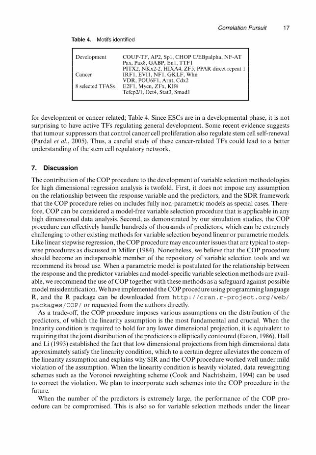
Table 4. Motifs identified

Development COUP-TF, AP2, Sp1, CHOP C/EBpalpha, NF-ATPax, Pax8, GABP, En1, TTF1PITX2, NKx2-2, HIXA4, ZF5, PPAR direct repeat 1

Cancer IRF1, EVI1, NF1, GKLF, WhnVDR, POU6F1, Arnt, Cdx2

8 selected TFASs E2F1, Mycn, ZFx, Klf4Tcfcp2/1, Oct4, Stat3, Smad1

for development or cancer related; Table 4. Since ESCs are in a developmental phase, it is notsurprising to have active TFs regulating general development. Some recent evidence suggeststhat tumour suppressors that control cancer cell proliferation also regulate stem cell self-renewal(Pardal et al., 2005). Thus, a careful study of these cancer-related TFs could lead to a betterunderstanding of the stem cell regulatory network.

7. Discussion

The contribution of the COP procedure to the development of variable selection methodologiesfor high dimensional regression analysis is twofold. First, it does not impose any assumptionon the relationship between the response variable and the predictors, and the SDR frameworkthat the COP procedure relies on includes fully non-parametric models as special cases. There-fore, COP can be considered a model-free variable selection procedure that is applicable in anyhigh dimensional data analysis. Second, as demonstrated by our simulation studies, the COPprocedure can effectively handle hundreds of thousands of predictors, which can be extremelychallenging to other existing methods for variable selection beyond linear or parametric models.Like linear stepwise regression, the COP procedure may encounter issues that are typical to step-wise procedures as discussed in Miller (1984). Nonetheless, we believe that the COP procedureshould become an indispensable member of the repository of variable selection tools and werecommend its broad use. When a parametric model is postulated for the relationship betweenthe response and the predictor variables and model-specific variable selection methods are avail-able, we recommend the use of COP together with these methods as a safeguard against possiblemodel misidentification. We have implemented the COP procedure using programming languageR, and the R package can be downloaded from http://cran.r-project.org/web/packages/COP/ or requested from the authors directly.

As a trade-off, the COP procedure imposes various assumptions on the distribution of thepredictors, of which the linearity assumption is the most fundamental and crucial. When thelinearity condition is required to hold for any lower dimensional projection, it is equivalent torequiring that the joint distribution of the predictors is elliptically contoured (Eaton, 1986). Halland Li (1993) established the fact that low dimensional projections from high dimensional dataapproximately satisfy the linearity condition, which to a certain degree alleviates the concern ofthe linearity assumption and explains why SIR and the COP procedure worked well under mildviolation of the assumption. When the linearity condition is heavily violated, data reweightingschemes such as the Voronoi reweighting scheme (Cook and Nachtsheim, 1994) can be usedto correct the violation. We plan to incorporate such schemes into the COP procedure in thefuture.

When the number of the predictors is extremely large, the performance of the COP pro-cedure can be compromised. This is also so for variable selection methods under the linear


model. Lately, Fan and Lv (2008) have advocated a two-step approach to attack so-called ultra-high dimensionality. The first step is to perform screening to reduce the dimensionality fromultrahigh to high or moderately high, and then, in the second step, variable selection methodsare applied to identify the true predictors. The same approach can be used for variable selectionunder the SDR framework. More precisely, we can apply the forward COP procedure, whichis simply the COP procedure with the deletion step removed, to reduce the dimensionality ofa problem from ultrahigh to moderately high. The forward COP procedure is much easier toimplement and computationally more efficient than the COP procedure. Then, the usual COPprocedure is applied to the reduced data to select the true predictors. This approach is currentlyunder investigation and the results will be reported in a future publication.

Acknowledgements

We thank Xuming He, Steve Portnoy and John Marden for helpful suggestions. This workwas supported by National Institutes of Health grant U01 ES016011, a Department of Energygrant from the Office of Science (Biological and Environmental Research) and National ScienceFoundation grant DMS 1120256 to WZ, National Institues of Health grant R01-HG02518-02and National Science Foundation grant DMS 1007762 to JL and National Science Foundationgrant DMS 0707004 to YZ.

Appendix A

A.1. Proof of proposition 1Let S⊥.B/ denote the space of vectors such that, for any ρ ∈ S⊥.B/ and any β ∈ S.B/, ρ′Σβ = 0: LetS⊥.K/ be the space of vectors such that for any ρ∈S⊥.K/ ρ′Σηk =0 for k =1, . . . , K: We shall show thatS⊥.B/⊆S⊥.K/, which means, for any ρ∈S⊥.B/, P.ρ/=0: First, because, for any T , T.Y/⊥η′X|B′X, then

cov{T.Y/, η′X}=E{T.Y/η′X}=E[E{T.Y/|B′X}E.η′X|B′X/]:

Because of the linearity condition, for any ρ∈S⊥.B/, E.ρ′X|B′X/=c1β′1X+ . . .+cKβ′

KX, where c1, . . . , cK

are linear coefficients. In addition, since cov.ρ′X, β′kX/=0 for k=1, . . . , K, E.ρ′X|B′X/=0: Consequently,

corr2{T.Y/, ρ′X}= cov2{T.Y/, ρ′X}var{T.Y/}var.ρ′X/

=0,

P.ρ/=0 and S⊥.B/⊆S⊥.K/: Proposition 1 holds.

A.2. Proof of theorem 1Without loss of generality, we let A= {1, . . . , d} and t = d + 1: Let X.j/ be the vector of n independentidentically distributed observations of the jth variable for j =1, . . . , d +1. We assume that the predictorshave been centred to have zero sample mean. Denote Xn×j = .X.1/, . . . , X.j// for j =d, d +1: We let

M.j/ =

H∑h=1

nh

nX

.j/Th X

.j/

h for j =d, d +1

where X.j/

h .j = d, d + 1/ is the average of the first j variables for those individuals whose responses fallinto the hth slice Sh, h=1, . . . , H: Let nh be the number of observations in the hth slice, h=1, . . . , H: Letλi

.j/ be the ith largest eigenvalue of Σj−1

M.j/ for j = d, d + 1, where Σj is the sample variance–covariancematrix of Xn×j: It is difficult to see the asymptotic distribution of λi

.d+1/ − λi.d/ for i = 1, . . . , K directly

based on Σj−1

M.j/ for j =d, d +1: We did some transformations such that the transformed Σj−1

M.d/ (witheigenvalues unchanged) is a submatrix of the transformed Σj

−1M.d+1/.

Let

γn×1 = .γ1, . . . , γn/T = 1σ

{I −Xn×d.XTn×dXn×d/−1XT

n×d}X.d+1/,


where σ2 is the sample variance of {I −Xn×d.XTn×dXn×d/−1XT

n×d}X.d+1/: Denote γh =n−1h Σyi∈Sh

γi: Let γ =Xd+1 −E.Xd+1|X1, . . . , Xd/, and γn×1 be the n regression error terms of the n observed Xd+1 on X1, . . . , Xd:Then γn×1 are independent and identically distributed with mean 0 and a finite variance. Under the nullhypothesis H0 :ηd+1, i =0, i=1, . . . , K, we have E.γ|y/=E{E.γ|X1, . . . , Xd/|y}=0 for any y. Let γ be themean of γn×1: Then

γn×1 = .γ1, . . . , γn/T = 1σ

{I −Xn×d.XTn×dXn×d/−1XT

n×d}.γn×1 − γ/:

With transformations on Σ−1j M

.d/, we showed that λ

.d+1/

i − λ.d/

i for i = 1, . . . , K equals a squared lin-ear combination of γh: Thus, we just need to show that .γ1, . . . , γH / converges to a multivariate nor-mal distribution, and we complete the proof. Let .z1, . . . , zd/′ =Σd

−1=2.x1, . . . , xd/′. Define four matrices,AH×H , BH×d , Ed×d and ΓH×d , where AH×H =diag{var.γ|y ∈S1/, . . . , var.γ|y ∈SH /}=σ2, the .h, j/th entryof BH×d is

√ph cov.zjγ, γ|y∈Sh/=σ2, the .j, j′/th entry of Ed×d equals cov.zj′γ, zjγ/=σ2, the .h, j/th entry

of ΓH×d is√

ph E.zj|y ∈Sh/ and σ2 = limn→.σ2/=var.γ/: Let Υ be a d ×d matrix and

Υ=ΓTH×dAH×HΓH×d −ΓT

H×dBH×dΓTH×dΓH×d −ΓT

H×dΓH×dBTH×dΓH×d +ΓT

H×dΓH×dEd×dΓTH×dΓH×d :

Define Q to be a d ×K matrix with jth column qj=√{λ.d/

j .1−λ.d/j /}, where qj is the the jth eigenvector of

the limiting matrix limn→∞.Σ−1=2d M

.d/Σ

−1=2d /, and λ.d/

j = limn→∞.λj.d//: Then WKt = QTΥQ:

A.3. Proof of corollary 1With an additional condition that E.γ2|X1, . . . , Xd/ is constant, we can show that the asymptotic variancematrix of .γ1, . . . , γH / adopts a special form, with which the asymptotic standard χ2-distribution can bederived.

A.4. Proof of theorem 2Without loss of generality, we let A={X1, . . . , Xd}: Following the notation that was used in theorem 1,let γj =Xj −E.Xj|Xi, i∈A/ for j ∈Ac, and

γj = .γj,1, . . . , γj,n/′ = 1σj

{In −Xn×d..Xn×d/′Xn×d/−1.Xn×d/′}X.j/:

Let γjh =n−1

h Σyi∈Shγj, i: Similarly to the proof of theorem 1, we basically show γ

jh for j =d + 1, . . . , p and

h=1, . . . , H converge to a multivariate normal distribution.

A.5. Proof of theorem 3We use the same notation as defined in the proof of theorem 2. Let γ

jh =n−1

h Σyi∈Shγj, i: Let λ

.d/

k be definedas in the proof of theorem 1. First, for any t, COPA+t

1:K �n.ΣKk=1 λ

.d+1/

k −ΣKk=1 λk

.d//, and

∣∣∣ K∑k=1

λ.d+1/

k −K∑

k=1λ

.d/

k

∣∣∣� ∣∣∣ K∑k=1

.λ.d+1/k −λ.d/

k /∣∣∣− ∣∣∣ K∑

k=1.λ.d+1/

k − λ.d+1/

k /∣∣∣− ∣∣∣ K∑

k=1.λ.d/

k − λ.d/

k /∣∣∣:

Since X follows a multivariate normal distribution, from Li (1991), λ.d/k =λ.d+1/

k =0 for k>K; then

K∑k=1

.λ.d+1/k −λ.d/

k /= limn→∞

{tr.Ω.d+1/

/− tr.Ω.d/

/}= limn→∞

{H∑

h=1

nh

n.γ

jh/2

}=

H∑h=1

ph

E2.γj|y ∈Sh/

σ2j

:

We need to use the two lemmas 1 and 2 that are stated below. The proofs of the two lemmas are omittedhere. From lemma 1,

maxt∈Ac∩T

{n

(K∑

k=1λ

.d+1/

k −K∑

k=1λ

.d/

k

)}�ωH n1−ξ0

τ 2min

τmax−

∣∣∣ K∑k=1

n.λ.d+1/k − λ

.d+1/

k /∣∣∣− ∣∣∣ K∑

k=1n.λ.d/

k − λ.d/

k /∣∣∣:

Then, as long as


maxA⊆{1,:::,p}

{n

∣∣∣∣∣K∑

k=1.λ.d/

k − λ.d/

k /

∣∣∣∣∣}

�ϑn1−ξ0 =2,

we have

minA:Ac∩T �=∅

maxt∈Ac∩T

.COPA+t1:K /�ϑn1−ξ0 :

From lemma 2,

P

(max

A⊆{1,:::,p}

∣∣∣ K∑k=1

λ.d/k −

K∑k=1

λ.d/

k

∣∣∣>ϑn−ξ0

2

)�2Kp.p+1/C1 exp

(−C2n

1−2ξ0τ 2

minϑ2

256K2p2

):

Under condition 8, since p=o.n�0 / with 2�0 +2ξ0 <1, P.maxA⊆{1,:::,p} |ΣKk=1 λ.d/

k −ΣKk=1 λ

.d/

k |>ϑn−ξ0 =2/→0, and P{minA:Ac∩T �=∅ maxt∈Ac∩T .COPA+t

1:K /�ϑn1−ξ0}→1:

A.6. Proof of theorem 4Since ∣∣∣ K∑

k=1λ

.d+1/

k −K∑

k=1λ

.d/

k

∣∣∣� ∣∣∣ K∑k=1

.λ.d+1/k −λ.d/

k /∣∣∣+ ∣∣∣ K∑

k=1.λ.d+1/

k − λ.d+1/

k /∣∣∣+ ∣∣∣ K∑

k=1.λ.d/

k − λ.d/

k /∣∣∣,

and, with T ⊆A, |ΣKk=1 .λ.d+1/

k −λ.d/k /|= 0, then, from lemma 2, P.maxA⊆{1,:::,p} |ΣK

k=1 λ.d/k −ΣK

k=1λ.d/

k | >"/→0 for ">Cn�0−1=2 and theorem 4 holds.

Lemma 1. Under the same conditions as in theorem 3, for any A⊆{1, . . . , p} and Ac ∩T �=∅,

maxj∈Ac∩T

{H∑

h=1ph E2.γj|y ∈Sh/=σ2

j

}� τ 2

minωH n−ξ0 =τmax > 0:

Lemma 2. Under the same conditions as in lemma 1,

P(

maxA⊆{1,:::,p}

∣∣∣ K∑k=1

λ.d/k −

K∑k=1

λ.d/

k

∣∣∣>")

�2Kp.p+1/C1 exp(

−C2nτ 2

min"2

64K2p2

):

A.7. Proof of theorem 5For coherence, we use the same notation as defined in the proof of theorem 1. Without loss of generality,let A={1, . . . , d} and t = d + 1: Under the assumption that Xn×.d+1/ has a multivariate normal distribu-tion, we derive the limiting value of .ΣK

k=1 λ.d+1/

k −ΣKk=1 λ

.d/

k / as n →∞ for fixed slices. Let ΞK×K be thevariance–covariance matrix of vK:

Because {X1, . . . , Xd+1} follow a multivariate normal distribution, we have γ = Xd+1 − ρ0 + Σdi=1 ρiXi

and γ ∼N.0, σ2d+1/ where the ρi are the coefficients. Since we assume that the response depends only on K

linear combinations of Xn×.d+1/, Ω.d+1/

and Ω.d/

have at most K non-zero eigenvalues, and

K∑k=1

λ.d+1/

k

tr.Ω.d+1/

/

P→1,

K∑k=1

λ.d/

k

tr.Ω.d/

/

P→1,

K∑k=1

λ.d+1/

k −K∑

k=1λ

.d/

k

tr.Ω.d+1/

/− tr.Ω.d/

/

P→1:


We have the following three results.

(a) tr.Ω.d+1/

/− tr.Ω.d/

/=ΣHh=1 nh.γh/2=n:

(b) γh→PE.γ|y ∈Sh/=σd+1, h=1, . . . , H:(c) Since E.γ|vK/= ηt,AΞ−1

K×KvK, then

E.γ|y ∈Sh/=E{E.γ|vK/|y ∈Sh}= η′t,AΞ−1

K×KLH ,K:

Combining results (a)–(c) we have ΣHh=1 nh.γh/2=n→Pη′

t,AΞ−1K×KMH ,KΞ−1

K×Kηt,A: Since Ξ−1K×K = IK×K,

K∑k=1

λA+t

k −K∑

k=1λ

Ak

P→ 1σ2

d+1

η′t,AMH ,Kηt,A,

and theorem 5 holds.

A.8. Proof of proposition 2Note that η′MH ,Kη =var{E.η′vK|y ∈Sh/} and

var{E.η′vK|y ∈S′h′/}=var{E.η′vK|y ∈Sh/}+var[var{E.η′vK|y ∈S′

h′/|Sh}]:

Thus, proposition 2 holds.

References

Bondell, H. D. and Li, L. (2009) Shrinkage inverse regression estimation for model-free variable selection. J. R.Statist. Soc. B, 71, 287–299.

Boyer, L. A., Lee, T. I., Cole, M. F., Johnstone, S. E., Levine, S. S., Zucker, J. P., Guenther, M. G., Kumar, R.M., Murray, H. L., Jenner, R. G., Gifford, D. K., Melton, D. A., Jaenisch, R. and Young, R. A. (2005) Coretranscriptional regulatory circuitry in human embryonic stem cells. Cell, 122, 947–956.

Cai, J., Xie, D., Fan, Z., Chipperfield, H., Marden, J., Wong, W. H. and Zhong, S. (2010) Modeling co-expressionacross species for complex traits: insights to the difference of human and mouse embryonic stem cells. PLOSComput. Biol., 6, article e1000707.

Chen, C.-H. and Li, K.-C. (1998) Can SIR be as popular as multiple linear regression? Statist. Sin., 8, 289–316.Chen, X., Xu, H., Yuan, P., Fang, F., Huss, M., Vega, V. B., Wong, E., Orlov, Y. L., Zhang, W., Jiang, J., Loh, Y.

H., Yeo, H. C., Yeo, Z. X., Narang, V., Govindarajan, K. R., Leong, B., Shahab, A., Ruan, Y., Bourque, G.,Sung, W. K., Clarke, N. D., Wei, C. L. and Ng, H. H. (2008) Integration of external signaling pathways withthe core transcriptional network in embryonic stem cells. Cell, 133, 1106–1117.

Cleveland, W. (1979) Robust locally weighted regression and smoothing scatterplots. J. Am. Statist. Ass., 74,829–836.

Cloonan, N., Forrest, A. R. R., Kolle, G., Gardiner, B. B. A., Faulkner, G. J., Brown, M. K., Taylor, D. F., Steptoe,A. L., Wani, S., Bethel, G., Robertson, A. J., Perkins, A. C., Bruce, S. J., Lee, C. C., Ranade, S. S., Peckham,H. E., Manning, J. M., McKernan, K. J. and Grimmond, S. M. (2008) Stem cell transcriptome profiling viamassive-scale mRNA sequencing. Nat. Meth., 5, 613–619.

Conlon, E., Liu, X., Lieb, J. and Liu, J. (2003) Integrating regulatory motif discovery and genome-wide expressionanalysis. Proc. Natn. Acad. Sci. USA, 100, 3339–3344.

Cook, R. D. (1994) An Introduction to Regression Graphics. New York: Wiley.Cook, R. (2004) Testing predictor contributions in sufficent dimension reduction. Ann. Statist., 32, 1062–1092.Cook, R. D. and Nachtsheim, C. J. (1994) Reweighting to achieve elliptically contoured covariates in regression.

J. Am. Statist. Ass., 89, 592–599.Eaton, M. L. (1986) A characterization of spherical distributions. J. Multiv. Anal., 20, 272–276.Efron, B., Hastie, T., Johnstone, I. and Tibshirani, R. (2004) Least angle regression. Ann. Statist., 32, 407–499.Fan, J. and Li, R. (2001) Variable selection via nonconcave penalized likelihood and its oracle properties. J. Am.

Statist. Ass., 96, 1348–1360.Fan, J. and Lv, J. (2008) Sure independence screening for ultrahigh dimensional feature space (with discussion).

J. R. Statist. Soc. B, 70, 849–911.Fan, J. and Lv, J. (2010) A selective overview of variable selection in high dimensional feature space. Statist. Sin.,

20, 101–148.Friedman, J. H. (2007) Pathwise coordinate optimization. Ann. Appl. Statist., 1, 302–332.Friedman, J. H. and Tukey, J. W. (1974) A projection pursuit algorithm for explanatory data analysis. IEEE Trans.

Comput. C, 23, 881–889.Fung, W., He, X., Liu, L. and Shi, P. (2002) Dimension reduction based on canonical correlation. Statist. Sin.,

12, 1093–1114.


Hall, P. and Li, K.-C. (1993) On almost linearity of low dimensional projections from high dimensional data.Ann. Statist., 21, 867–889.

Huber, P. J. (1985) Projection pursuit. Ann. Statist., 13, 435–475.Johnson, D. S., Mortazavi, A., Myers, R. M. and Wold, B. (2007) Genome-wide mapping of in vivo protein-DNA

interactions. Science, 316, 1497–1502.Li, K.-C. (1991) Sliced inverse regression for dimension reduction. J. Am. Statist. Ass., 86, 316–327.Li, L. (2007) Sparse sufficient dimension reduction. Biometrika, 94, 603–613.Li, L., Cook, R. D. and Nachtsheim, C. J. (2005) Model-free variable selection. J. R. Statist. Soc. B, 67, 285–299.Matsuda, T., Nakamura, T., Nakao, K., Arai, T., Katsuki, M., Heike, T. and Yokota, T. (1999) STAT3 activation

is sufficient to maintain an undifferentiated state of mouse embryonic stem cells. EMBO J., 18, 4261–4269.Miller, A. J. (1984) Selection of subsets of regression variables (with discussion). J. R. Statist. Soc. A, 147, 389–425.Mortazavi, A., Williams, B. A., McCue, K., Schaeffer, L. and Wold, B. (2008) Mapping and quantifying mam-

malian transcriptomes by RNA-Seq. Nat. Meth., 5, 621–628.Nagalakshmi, U., Wang, Z., Waern, K., Shou, C., Raha, D., Gerstein, M. and Snyder, M. (2008) The transcrip-

tional landscape of the yeast genome defined by RNA sequencing. Science, 320, 1344–1349.Ouyang, Z., Zhou, Q. and Wong, W. H. (2009) Chip-seq of transcription factors predicts absolute and differential

gene expression in embryonic stem cells. Proc. Natn. Acad. Sci. USA, 106, 21521–21526.Pardal, R., Molofsky, A. V., He, S. and Morrison, S. J. (2005) Stem cell self-renewal and cancer cell proliferation

are regulated by common networks that balance the activation of proto-oncogenes and tumor suppressors.Cold Spring Harb. Symp. Quant. Biol., 70, 177–185.

Shao, J. (1998) An asymptotic theory for linear model selection (with discussion). Statist. Sin., 7, 221–264.Tibshirani, R. (1996) Regression shrinkage and selection via the lasso. J. R. Statist. Soc. B, 58, 267–288.Wang, H. (2009) Forward regression for ultra-high dimensional variable screening. J. Am. Statist. Ass., 104,

1512–1524.Wilhelm, B. T., Marguerat, S., Watt, S., Schubert, F., Wood, V., Goodhead, I., Penkett, C. J., Rogers, J. and Bahler,

J. (2008) Dynamic repertoire of a eukaryotic transcriptome surveyed at single-nucleotide resolution. Nature,453, 1239–1243.

Zeng, P. and Zhu, Y. (2010) An integral transform method for estimating the central mean and central subspaces.J. Multiv. Anal., 101, 271–290.

Zhong, W., Zeng, P., Ma, P., Liu, J. and Zhu, Y. (2005) Regularized sliced inverse regression for motif discovery.Bioinformatics, 21, 4169–4175.

Zhou, J. and He, X. (2008) Dimension reduction based on constrained cannonical correlation and variable filter-ing. Ann. Statist., 36, 1649–1668.

Zhu, L., Miao, B. and Peng, H. (2006) On sliced inverse regression with high-dimensional covariates. J. Am.Statist. Ass., 101, 630–643.

Zou, H. (2006) The adaptive lasso and its oracle properties. J. Am. Statist. Ass., 101, 1418–1429.

correlation pursuit:forward stepwise variable selection ...junliu/techrept/12folder/cop2012.pdf ·...

Documents