corruption and growth in asean countries: a non-linear

International Journal of Academic Research in Business and Social Sciences

Vol. 1 0 , No. 3, March, 2020, E-ISSN: 2222-6990 © 2020 HRMARS

347

Full Terms & Conditions of access and use can be found at

http://hrmars.com/index.php/pages/detail/publication-ethics

Corruption and Growth in ASEAN Countries: A Non-Linear Investigation Tiang Jang Haw, Jerome Kueh & Shirly Wong Siew Ling

To Link this Article: http://dx.doi.org/10.6007/IJARBSS/v10-i3/7055 DOI:10.6007/IJARBSS/v10-i3/7055

Received: 01 February 2020, Revised: 20 February 2020, Accepted: 10 March 2020

Published Online: 30 March 2020

In-Text Citation: (Haw et al., 2020) To Cite this Article: Haw, T. J., Kueh, J., & Ling, S. W. S. (2020). Corruption and Growth in ASEAN Countries: A

Non-Linear Investigation. International Journal of Academic Research in Business and Social Sciences, 10(3), 347–369.

Copyright: © 2020 The Author(s)

Published by Human Resource Management Academic Research Society (www.hrmars.com) This article is published under the Creative Commons Attribution (CC BY 4.0) license. Anyone may reproduce, distribute, translate and create derivative works of this article (for both commercial and non-commercial purposes), subject to full attribution to the original publication and authors. The full terms of this license may be seen at: http://creativecommons.org/licences/by/4.0/legalcode

Vol. 10, No. 3, 2020, Pg. 347 - 369

http://hrmars.com/index.php/pages/detail/IJARBSS JOURNAL HOMEPAGE

http://creativecommons.org/licences/by/4.0/legalcode



348

Corruption and Growth in ASEAN Countries: A Non-

Linear Investigation

Tiang Jang Haw, Jerome Kueh & Shirly Wong Siew Ling Faculty of Economics and Business, Universiti Malaysia Sarawak, Malaysia

94300 Kota Samarahan, Sarawak, Malaysia Email: [email protected]

Abstract This paper examined the nexus between corruption and economic growth of the Association of Southeast Asian Nations (ASEAN) countries covering the period from 1996 to 2018. Most of the ASEAN countries experiencing high level of corruption associated with robust economic growth performance. This phenomenon is opposite against the prevalent proposition of negative linkage between corruption and economic growth. Therefore, a non-linearity analysis has been incorporated to cover the changes in the effect of corruption on economic growth. This finding revealed there is a significant U-shaped relationship between control of corruption and economic growth of ASEAN countries. In other words, corruption may indirectly facilitate the growth until certain threshold level, ultimately, corruption is substantially reducing growth as corruption level under control. Empirical results indicate that the threshold level of corruption is approximately 1.84 on a 5-point scale of corruption control. This shows that corruption will be detrimental to growth when the corruption level is beyond the threshold level. The speed of adjustment implies that ASEAN countries was vulnerable to the variations as it takes longer time to adjust to long-run equilibrium, particularly on economic growth, trade openness, and inflation. The granger causality test denotes the causality between control of corruption and other variables are mutually complementary. Keywords: Corruption, Economic Growth, ASEAN Countries, Non-linearity Analysis, Threshold. Introduction

Corruption is a common phenomenon occurs around worldwide. Corruption generally defined as “abuse of public power for private gain” (Bhargava, 2005; Johnston, 1986; Transparency International, 2018). The corruption is fundamentally recognized as illegitimately and immorally behaviour that severally affecting human community. In other hands, corruption possess multiple causes and effects while taking different role under a different context (Papaconstantinou et al., 2013). Besides that. Kennedy (1997) stated that there is no standard definition of corruption as it could treated as righteous if the prevalent norms and regulations are unjust.



349

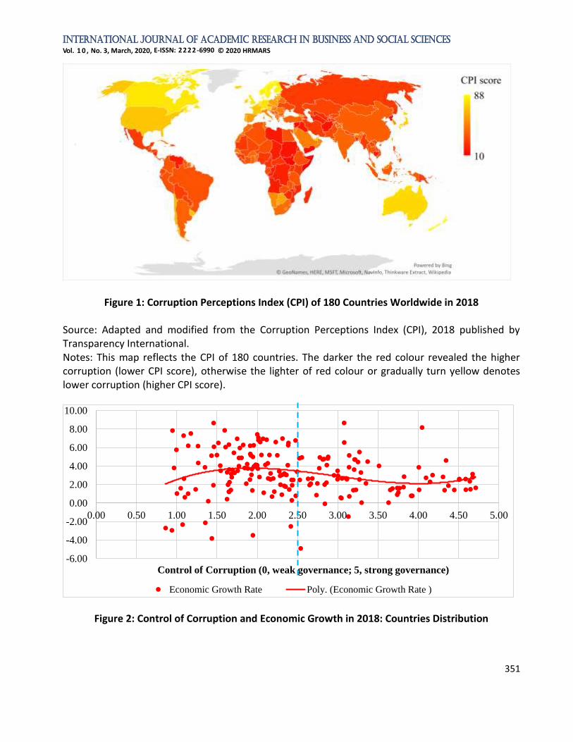
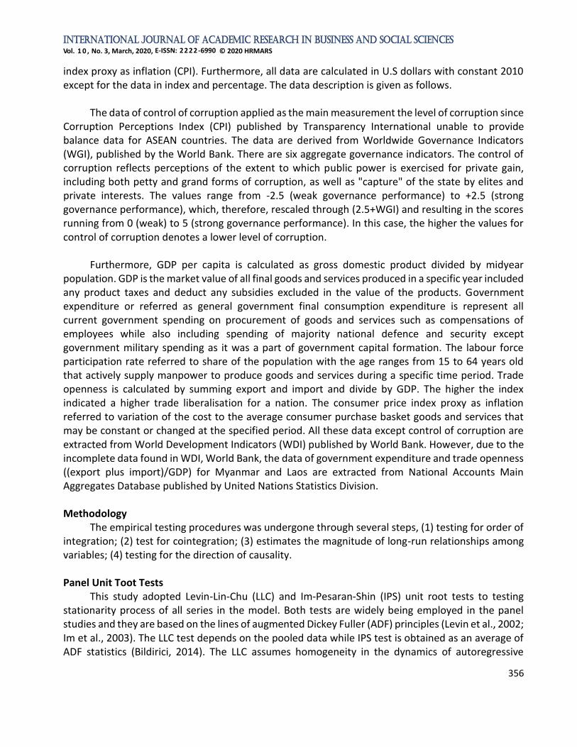
Throughout the world, majority countries experiencing pervasiveness corruption without any progressive improvement in recent years. According to the Corruption Perceptions Index (CPI) published by Transparency International in 2018 (refer to Figure 1), it represents over 120 out of 180 countries around the world scoring an average of 43 CPI (0, most corrupt; 100, very clean), which reflected an overall status of weak governance in controlling corruption worldwide. Furthermore, corruption has drawn widespread advertence amongst developing countries since expansion of press freedom and democracy in recent year (Pulok & Ahmed, 2017; Paul, 2010). Pervasiveness corruption is treated as major obstacle to the health of democracies as a weak democratic foundation provide opportunity for corruption to thrive (Transparency International Secretariat, 2019). Meanwhile, corruption treated as main deterrence to ending extreme poverty by 2030 and promotes the shared prosperity amongst 40% of poorest people in developing countries (The World Bank, 2018). By linking the economic growth rate and level of controlling corruption (refer to Figure 2), it revealed a paradox relationship between corruption levels and economic growth as high level of corruption associated with the robust economic growth for most of the countries. A larger number of countries score below 2.5 of governance performance in controlling corruption while achieves economic growth rate 3.0 percent and above. The similar phenomenon also discovered in the Southeast Asia countries or referred as Association of the Southeast Asian Nations (ASEAN) member states. By referring to Figure 3, most of the ASEAN countries having an average performance in controlling corruption less than 2.5 while economic growth rate above 5 percent in over a past decade. Therefore, the phenomenon discovered is opposite with the prevalent propositions of detrimental linkage of corruption and economic growth.

Southeast Asia as one of the most economically and politically diverse regions worldwide. It

comprised of some of the richest and emerging economies as well as some of poorest people around the world while exist of various government represented by a monarchy, autocracy, military government and democracy (Transparency International, 2015). Besides that, ASEAN is the 6th largest economies around the world and 3rd largest economies in Asia while having third-largest population after China and India with over more than half young population (The ASEAN Secretariat, 2017a, 2017b). In 2018, ASEAN member countries achieved total GDP of nearly 2.99 trillion US dollars, with a real GDP growth rate of 5.2%, and are expected to continue to grow at 4.5% in the next two years (The ASEAN Secretariat, 2019). Furthermore, pervasiveness corruption at ASEAN countries believes to deter the aspirations of sustainable economic growth and development, either at the individual's countries or regional level. A few surveys report in ASEAN countries have revealed a situation where corruption is widely perceived in the public, public administration and business environment (see example, Enterprise Surveys, 2019; Pring, 2017). Apart from that, other issues such as historical impact of brutal ruling regime in the past, weak governance and nation integrity system, weakness enforcement and monitoring system in safeguard the natural resources, the imbalance for prosecution and arrest as well as a low conviction rate for discipline related offender, informal sectors' ecosystem & civil tension, the weak regulatory framework and civil society, and exist of stated-restricted news media system (see examples, Amin, 2016; Corruption Eradication Commission [KPK], 2015; GAN Integrity, 2016, 2017a, 2017b; Gregory, 2016; Hashim, 2017; Khaing, 2015; Stokke et al., 2018; Transparency International Cambodia, 2014). All these above are the several issues that have mentioned related to most of the ASEAN countries that closely linked to widespread corruption.



350

Thence, the existence of a vicious cycle of corruption severely deters the initiative to act against corruption since it is deep-rooted at all level and eventually corrodes the country's health. This will become an obstacle to promoting a peaceful, justice, and strong institutions, that is 16th out of 17 Sustainable Development Goals (SDGs) formulated by the United Nations. The SDGs emphasizes a holistic approach to achieving sustainable development by 2030 (see example, United Nations, n.d.; United Nations Office on Drugs and Crime [UNODC], 2019).

Although the empirical evidence of detrimental effect of corruption on growth has well-

established in the conventional empirical studies. However, some empirical literature did suggest that impact of corruption to economic growth or development might subject to certain circumstances. Corruption has been discovered to be less deleterious or even positive to growth particularly at a weak governance environment, low level of economic development, inefficient rule of law and so forth. The empirical analysis also extended to non-linearity analysis to examine the effect changes of the level of corruption on growth or vice versa. The empirical analysis of non-linearity between corruption and economic growth or development gradually to be acknowledged to provide evidence in explaining the difference of the impact of corruption on the nation’s economy.

This study examines the relationship between corruption and economic growth of ASEAN

countries from 1996 to 2018 by employed a panel data analysis comprised of panel unit root, panel cointegration, panel ARDL estimations, and panel causality. The study aims to offer a systematic analysis of the long-run relationship and causality in growth and corruption. Most importantly, the analysis extended by covers a non-linearity between corruption and growth in a 2nd-degree polynomial framework. It noteworthy to mention the limited empirical studies in ASEAN countries provide less supportive evidence to explain the phenomenon discovered in the region. The analysis was then incorporated with non-linearity analysis to provide a more comprehensive insight regarding the effect changes of corruption on growth in the ASEAN context. With the inclusion of non-linearity analysis with the threshold value, it will contribute to the policies formulation by providing a more informative reference. The paper is structured as followed. Section 2 mentioned the literature review. Section 3 describes the models, data, and methodology. Results and discussions are presented in Section 4 followed by the conclusion and policy recommendation described in Section 5.



351

Figure 1: Corruption Perceptions Index (CPI) of 180 Countries Worldwide in 2018 Source: Adapted and modified from the Corruption Perceptions Index (CPI), 2018 published by Transparency International. Notes: This map reflects the CPI of 180 countries. The darker the red colour revealed the higher corruption (lower CPI score), otherwise the lighter of red colour or gradually turn yellow denotes lower corruption (higher CPI score).

Figure 2: Control of Corruption and Economic Growth in 2018: Countries Distribution

-6.00

-4.00

-2.00

0.00

2.00

4.00

6.00

8.00

10.00

0.00 0.50 1.00 1.50 2.00 2.50 3.00 3.50 4.00 4.50 5.00

Control of Corruption (0, weak governance; 5, strong governance)

Economic Growth Rate Poly. (Economic Growth Rate )



352

Sources: Adapted and modified from Worldwide Governance Indicators (WGI) and World Development Indicators (WDI) published by World Bank. Notes: The x-axis and y-axis represented governance level of control of corruption and economic growth rate respectively. The countries distribution comprised of 193 countries and regions worldwide. The middle dot line in blue colour represents the middle score of control of corruption which is 2.5.

Figure 3: Average Control of Corruption and Economic Growth of ASEAN Countries from 2009 to 2018

Sources: Adapted and modified from Worldwide Governance Indicators (WGI) and World Development Indicators (WDI) published by World Bank. Literature Review

Even though the insightful literature on the impact of corruption to growth or development arose in the 1960s, but the explosion of the analytical study upsurge in the 1990s due to the development of indicators of corruption that propelled corruption studies (Ata & Arvas, 2011). Furthermore, there is existence of mixed relationship between corruption and economic growth or development. The findings can be categorized into three aspect namely, “sand the wheels”, “grease the wheels”, and non-linear relationships between corruption and growth.

Firstly, the sand the wheels' hypothesis corresponding with the negative relationships between

corruption and growth that are well-established in the empirical findings. The early analytical works by Mauro (1995) found out corruption adversely affect the economic growth of 69 countries and reduce investment. The findings revealed one-standard-deviation improvement in the corruption increase the GDP per capita growth rate and investment rate by 1.3 % and 2.9 %, respectively. In other hands, Méon and Sekkat (2005) are argued that the detrimental effect of corruption on growth

1.31 1.45 1.481.95 1.95 1.98 2.12

2.673.21

4.63

6.35

7.53 7.54

5.825.38

6.15

3.32

4.73

-0.06

4.68

-1.00

0.00

1.00

2.00

3.00

4.00

5.00

6.00

7.00

8.00

Control of Corruption Economic Growth Rate (%)



353

is nothing to do with its impact on investment. And the impact of corruption on investment is subject to the quality of governance as good governance can mitigate the cost of corruption. D’Agostino et al (2012) discovered that corruption magnifies the impact of military burden and reduce the benign effect of public investment on growth. A panel analysis in ASEAN countries by Aziz and Sundarasen (2015) confirm the significant adverse effect of corruption and armed conflict to the economic growth of ASEAN-7 countries from 2000 to 2009. Besides that, Azam and Emirullah (2014) have concluded the corruption has significant negative impact on economic growth by creating economic distortions, raising the cost of doing business and inequality. Bhattacharjee and Haldar (2015) highlighted that corruption negatively affect the economy of South Asia but its impact tends to be magnified under a weak institution. Mendonça and Baca (2017) found out the country with higher corruption experiencing an average decrease in the coefficient on public health expenditure and taxation by 21% and 68%, respectively. The study by Cieślik and Goczek (2018) implies lower corruption contribute to GDP per capita growth rate. And further mentioned the corruption takes a form of unpredictable distortion in the discretionary and uncertain use of government power which creates additional commercial cost and misallocation of resources that increase the economic burden. Moreover, Mo (2001), Abu et al. (2015), and Ghalwash (2014) provide evidence on the transmission channels in which corruption negatively affect growth is largely through political instability. Linhartova and Zidova (2016) have found out that corruption adversely affects the growth through household and government expenditures as well as an investment either directly or indirectly.

Furthermore, some studies revealed the impact of corruption on growth is less deleterious or

even positive which echoes with the grease the wheels' hypothesis. A very fundamental statement is that corruption treat as “speed money”, to simplify the rigid procedures, increase bureaucratic efficiency which contributes to productivity that eventually contributes growth. Meanwhile, corruption replace the prevalent norm and regulations to serve as alternatives under an inefficient governance environment which turn corruption become a pervasive phenomenon. Méon and Weill (2010) discover that corruption is less detrimental or even positively related to efficiency in the countries with a weak institutional framework. But the authors highlighted those result pertained to the effect of corruption on aggregate efficiency as corruption still essentially deleterious to the accumulation of factors of production. The study by Huang (2012) and Ondo (2017) indicated corruption have significant positive effect on growth in 10 Asian countries and EMCCA countries, respectively. A single country study on Bangladesh done by Paul (2010) revealed high corruption in one year leads to rising of growth in next year. Hence, the authors justified that unbalance implementation of reform policy in economic and institutional creates a situation conducive to corruption particularly when the interaction increases between enterprises and public regulatory bodies for the taxes, utilities and permits. And corruption is lubricants the wheels of commerce in inefficient regulation that would otherwise dampen business development (Paul, 2010). The study by Ayaydın and Hayaloglu (2014) revealed that corruption is conducive to firm asset growth of 41 manufacturing firm in Turkey from 2008 to 2011. The authors stated that corruption is the price people are forced to pay due to the market failure while it facilitates the firm growth through surpass bureaucratic delay and increase government employee’s efficiency.



354

Apart from the monotonic relationship between corruption on growth, several studies have revealed a multidimensional effect of corruption on growth that incorporated both sand the wheels and grease the wheels’ hypothesis. The impact of corruption can be different before and after the respective threshold or any other aspects. Méndez and Sepúlveda (2006) have found out the low level of corruption contributes the economic growth whereas a high level of corruption reduces economic growth after control for some economic variables and limit the sample to free countries. Moreover, the study by Aidt et al. (2008) revealed the corruption-growth relationship is regime-specified as corruption adversely affects the growth in a regime with a high-quality institution but didn't affect the regime with low-quality institutions. In other hands, Bose et al. (2008) have provided evidence on the threshold at which corruption starts to inhibit the quality of public infrastructure (road, electricity, and water supply) in 125 countries. Moreover, Heckelman and Powell (2010) found out corruption is beneficial on growth when the degree of economic freedom is low especially in government size, freedom to trade, and regulation of credit, labour, and business. Interestingly, the growth-enhancing effect of corruption was reduced or even become negative when economic freedom rises as the size of government and regulations being improved. Conversely, Swaleheen (2011) provide evidence corruption is not always growth-reducing at all levels and it differs across the countries. The findings even revealed corruption is growth-enhancing at a high level of incidence. A China firms-level study conducted by Wang and You (2012) indicated a threshold at which the corruption starts to reduce growth effect of financial development on enterprises is 0.19. which equivalent to 70 days a year for firms spent to interact with public officials. The authors further stated that the growth-enhancing effect of corruption only stay temporary and its effect will be reduced in the course of improvements of institutions. Furthermore, the study by Saha and Gounder (2013) revealed corruption level initially rising and start to decline when the country achieved an income level of USD 1339 which means higher economic development lead to a lower corruption level. Saha and Yap (2015) have found out that corruption facilitates tourism demand in least-corrupt countries whereas deterring tourism demand in high-corrupt countries. In addition, Mallik and Saha (2016) even discover a cubic relationship between corruption and growth as corruption is growth-reducing in the least-corrupt and high-corrupt countries, but growth-enhancing in medium-corrupt countries. The study by Saha and Ben Ali (2017) found out that the rising of income at early stages (less than US$ 8000) and mature stages (more than US$ 44,000) increases the corruption level but reduce corruption level at intermediate stages (US$ 8000 to US$ 44,000) in 16 Middle Eastern and North African (MENA) countries. Tomaszewski (2018) discovered both sand the wheel and grease the wheel' hypothesis in various innovation activities which further claimed that the two hypotheses are not mutually exclusive but complementary.

Models, Data, and Methodology Models

This study aims to examine the relationship between corruption and economic growth of ASEAN countries covering the period from 1996 to 2018 in annual basic. The ASEAN countries comprised of Brunei, Cambodia, Indonesia, Laos, Malaysia, Myanmar, Philippines, Singapore, Thailand, and Vietnam. The analysis extends to the non-linearity between corruption and economic growth by investigating whether exists the effect changes of the level of corruption on growth. This intends testing nexus between corruption and economic growth is non-linear and by investigating



355

the veracity of the assumption that corruption is constantly giving detrimental effect on economic growth. The basic non-linearity model begins with the conventional linear model which specific as follow:

𝐺𝐷𝑃𝑃𝐶𝑖𝑡 = 𝛽0 + 𝛽1𝐶𝑂𝑅𝑅𝑖𝑡 + 𝛽2𝐺𝐸𝑖𝑡 + 𝛽3𝐿𝐴𝐵𝑖𝑡 + 𝛽4𝑇𝑂𝑖𝑡 + 𝛽5𝐶𝑃𝐼𝑖𝑡 + 휀𝑖𝑡 (1)

where GDPPC denotes to gross domestic product per capita, CORR denotes control of corruption, GE referred to government expenditure, LAB denotes the labour force participation rate, TO denotes trade openness, CPI denotes consumer price index proxy as inflation, 휀 is error term, 𝑖 refer to country and 𝑡 refer to time period. All variables are in the natural logarithm form.

Next, the model extended by examining the existence of a non-linear relationship between corruption and economic growth. Following the estimation technique that employed in the study by Méndez and Sepúlveda (2006), Swaleheen (2011), and Saha and Gounder (2013), a quadratic term or squared of control of corruption is added as explanatory variable in this typical econometric specification which expressed as follow:

𝐺𝐷𝑃𝑃𝐶𝑖𝑡 = 𝛽0 + 𝛽1𝐶𝑂𝑅𝑅𝑖𝑡 + 𝛽2𝐶𝑂𝑅𝑅𝑖𝑡2 + 𝛽3𝐺𝐸𝑖𝑡 + 𝛽4𝐿𝐴𝐵𝑖𝑡 + 𝛽5𝑇𝑂𝑖𝑡 + 𝛽6𝐶𝑃𝐼𝑖𝑡 + 휀𝑖𝑡 (2)

The non-linear relationship of control of corruption is reflected by the coefficient 𝛽1 and 𝛽2,

where the expected sign of 𝛽1and 𝛽2 is negative and positive, respectively. And, it represents a U-shaped relationship between control of corruption and economic growth. At a certain turning point, it denotes a growth-maximizing level of corruption and its effect is zero to growth. Hence, before the threshold, the effect of control of corruption on growth is negative (higher corruption levels) and only becomes positive (lower corruption levels) after the threshold of control of corruption. To measure the threshold at which corruption levels begin to decline and conducive to economic growth, the estimation of the threshold of this U-shaped relationship is written as follows:

𝐶𝑂𝑅𝑅∗ =−𝛽1

2𝛽2 (3)

where CORR* referred as the governance level of control of corruption at the threshold level, and 𝛽1and 2𝛽2 refers the coefficients of linear and quadratic term of control of corruption respectively. It noteworthy to mention that the control of corruption has been rescaled and ranges from 0 (weak governance performance) to 5 (strong governance performance). In other hands, a higher score of control of corruption revealed a lower level of corruption, otherwise lower score of control of corruption denotes a higher level of corruption. Data

This study applied the panel data in annual basic for all ASEAN member states from 1996 to 2018. These variables are commonly been found to be relevant to corruption levels and economic growth. The dependent variable is gross domestic product per capita (GDP per capita) proxy as economic growth. The control variables comprised of control of corruption (CORR), government expenditure (GE), labour force participation rate (LAB), trade openness (TO), and consumer price



356

index proxy as inflation (CPI). Furthermore, all data are calculated in U.S dollars with constant 2010 except for the data in index and percentage. The data description is given as follows.

The data of control of corruption applied as the main measurement the level of corruption since

Corruption Perceptions Index (CPI) published by Transparency International unable to provide balance data for ASEAN countries. The data are derived from Worldwide Governance Indicators (WGI), published by the World Bank. There are six aggregate governance indicators. The control of corruption reflects perceptions of the extent to which public power is exercised for private gain, including both petty and grand forms of corruption, as well as "capture" of the state by elites and private interests. The values range from -2.5 (weak governance performance) to +2.5 (strong governance performance), which, therefore, rescaled through (2.5+WGI) and resulting in the scores running from 0 (weak) to 5 (strong governance performance). In this case, the higher the values for control of corruption denotes a lower level of corruption.

Furthermore, GDP per capita is calculated as gross domestic product divided by midyear

population. GDP is the market value of all final goods and services produced in a specific year included any product taxes and deduct any subsidies excluded in the value of the products. Government expenditure or referred as general government final consumption expenditure is represent all current government spending on procurement of goods and services such as compensations of employees while also including spending of majority national defence and security except government military spending as it was a part of government capital formation. The labour force participation rate referred to share of the population with the age ranges from 15 to 64 years old that actively supply manpower to produce goods and services during a specific time period. Trade openness is calculated by summing export and import and divide by GDP. The higher the index indicated a higher trade liberalisation for a nation. The consumer price index proxy as inflation referred to variation of the cost to the average consumer purchase basket goods and services that may be constant or changed at the specified period. All these data except control of corruption are extracted from World Development Indicators (WDI) published by World Bank. However, due to the incomplete data found in WDI, World Bank, the data of government expenditure and trade openness ((export plus import)/GDP) for Myanmar and Laos are extracted from National Accounts Main Aggregates Database published by United Nations Statistics Division. Methodology

The empirical testing procedures was undergone through several steps, (1) testing for order of integration; (2) test for cointegration; (3) estimates the magnitude of long-run relationships among variables; (4) testing for the direction of causality. Panel Unit Toot Tests

This study adopted Levin-Lin-Chu (LLC) and Im-Pesaran-Shin (IPS) unit root tests to testing stationarity process of all series in the model. Both tests are widely being employed in the panel studies and they are based on the lines of augmented Dickey Fuller (ADF) principles (Levin et al., 2002; Im et al., 2003). The LLC test depends on the pooled data while IPS test is obtained as an average of ADF statistics (Bildirici, 2014). The LLC assumes homogeneity in the dynamics of autoregressive



357

coefficients for all panel numbers, while IPS assumes for heterogeneity in these dynamics which also referred as heterogenous panel unit root tests. The decision rule of stationarity is when the null hypothesis of unit root can be rejected at the conventional levels of significance. Panel Cointegration Test

Once the stationary of data is found, the testing procedures proceed with the cointegration test to examine the existence of long-run relationship of the panel data series. The study has incorporated the cointegration test developed by Pedroni (1999, 2004). Pedroni cointegration test comprised of 2 types of cointegration test to examine the existence of heterogeneity of cointegration vector based on the panel test (within-dimension approach) and group test (between-dimensional approach). For the panel test, it includes four statistics constituted by panel v-statistic, panel rho-statistic, panel PP-statistic and panel ADF-statistic. For the group test, it includes of three statistical namely, group rho-statistic, group PP-statistic and group ADF-statistic. A total of 7 tests are an asymptotically standard normal distribution given by the respective panel/group cointegration statistic. If there is 4 and more out of 7 cointegration statistics are statistically significant at convention levels of significance, then the null hypothesis of no cointegration can be rejected which implies the existence of cointegration among the panel data series.

Panel ARDL Estimation based on Pooled Mean Group (PMG) Estimator

This study employed panel ARDL model for panel long-run estimations which developed by Pesaran and Shin (1999) and Pesaran et al. (2001). Despite the existence of another long-run estimations method, the panel autoregressive distributed lag method is preferable over it is provide consistent estimates of the long-run coefficients that are asymptotically normal regardless data series is integrated at level I (0), first order, I (1) or mixed (Pesaran et al., 2001). This study was then incorporated with the pooled mean group (PMG) estimators as an alternative estimator to dealing with the dynamic heterogenous panels. The PMG estimators adapted the ARDL model for a panel setting by allowing the intercepts, short-run coefficients included with speed of adjustment and cointegrating terms to be vary across groups on the cross section while restraining the long run coefficients to be identical (Kisswani, 2017, Pesaran et al., 1999). A dynamic panel specification by including lags of the dependent variable and lagged independent variables, the autoregressive distributed lags (ARDL) for bound test is specified as following:

𝑌𝑖𝑡 = 𝑎𝑖 + ∑ 𝛿𝑖𝑗

𝑘

𝑖=1

𝑌𝑗,𝑡−𝑖 + ∑ 𝛽𝑖𝑡′ 𝑋𝑗,𝑡−𝑖

𝑞

𝑖=0

+ 휀𝑖𝑡 (4)

∆𝐺𝐷𝑃𝑃𝐶𝑖𝑡 = 𝛽1 + ∑ 𝛼𝑖𝑗∆𝐺𝐷𝑃𝑃𝐶𝑗,𝑡−𝑖

𝑘

𝑖=1

+ ∑ 𝛽𝑖𝑗∆𝐶𝑂𝑅𝑅𝑗,𝑡−𝑖

𝑘

𝑖=0

+ ∑ 𝑋𝑖𝑗∆𝐶𝑂𝑅𝑅𝑗,𝑡−𝑖2

𝑘

𝑖=0

+ ∑ 𝜙𝑖𝑗∆𝐺𝐸𝑗,𝑡−𝑖

𝑘

𝑖=0

+ ∑ 𝛿𝑖𝑗∆𝐿𝐴𝐵𝑗,𝑡−𝑖

𝑘

𝑖=0

+ ∑ 𝜗𝑖𝑗

𝑘

𝑖=0

∆𝑇𝑂𝑗,𝑡−𝑖 + ∑ 𝜑𝑖𝑗∆𝐶𝑃𝐼𝑗,𝑡−𝑖

𝑘

𝑖=0

+ 𝜃1𝐺𝐷𝑃𝑃𝐶𝑗,𝑡−1 + 𝜃2𝐶𝑂𝑅𝑅𝑗,𝑡−1 + 𝜃3𝐶𝑂𝑅𝑅𝑗,𝑡−12 + 𝜃4𝐺𝐸𝑗,𝑡−1 + 𝜃5𝐿𝐴𝐵𝑗,𝑡−1

+ 𝜃6𝑇𝑂𝑗,𝑡−1+𝜃7𝐶𝑃𝐼𝑗,𝑡−1 + 휀𝑗𝑡

(5)



358

where the 𝑖 refers to countries while 𝑡 refers to the time, ∆ refers to 1st variation factors, 𝑘 is the ideal lag length. The null hypothesis of no cointegration and the alternative hypothesis of cointegration exist can be examined through F-test which does not require typical allocation that depends on the data are fully I(0), fully I(1) or mixed; the number of the estimator; and whether the model have trend, intercept or both. Thus, the error correction equation is as follows:

𝐸𝐶𝑇𝑗,𝑡 = 𝐺𝐷𝑃𝑃𝐶𝑖𝑡 − 𝛽2 − ∑ 𝛼𝑖2𝐺𝐷𝑃𝑃𝐶𝑗,𝑡−𝑖

𝑘

𝑖=1

− ∑ 𝛽𝑖2𝐶𝑂𝑅𝑅𝑗,𝑡−𝑖

𝑘

𝑖=0

− ∑ 𝑋𝑖2𝐶𝑂𝑅𝑅𝑗,𝑡−𝑖2

𝑘

𝑖=0

− ∑ 𝜙𝑖2𝐺𝐸𝑗,𝑡−𝑖

𝑘

𝑖=0

− ∑ 𝛿𝑖2𝐿𝐴𝐵𝑗,𝑡−𝑖

𝑘

𝑖=0

− ∑ 𝜗𝑖2𝑇𝑂𝑗,𝑡−𝑖

𝑘

𝑖=0

− ∑ 𝜑𝑖2∆𝐶𝑃𝐼𝑗,𝑡−𝑖

𝑘

𝑖=0

(6)

where ECT referred to error correction term resulting from the long-run equilibrium relationship. Panel Causality Test

If two variables are cointegrated, then exist of the possibility to have at least one direction causal relationship (Granger, 1988). The analysis was extended by examine the existence of causality between variables. To test for panel causality, this study employed panel-based vector error correction model (VECM) with a dynamic error correction term. The Equation (7) displays the equation for economic growth represented by GDP per capita only for brevity where comparable equations for each of the right-hand side variables in (7) with the same general specification resulting in a total six-equation dynamic error correction model.

Δ𝐺𝐷𝑃𝑃𝐶𝑖𝑡 = α1𝑗 + ∑ 𝜃11𝑖𝑘Δ

𝑞

𝑘=1

𝐺𝐷𝑃𝑃𝐶𝑖𝑡−𝑘 + ∑ 𝜃12𝑖𝑘Δ

𝑞

𝑘=1

𝐶𝑂𝑅𝑅𝑖𝑡−𝑘 + ∑ 𝜃13𝑖𝑘Δ

𝑞

𝑘=1

𝐺𝐸𝑖𝑡−𝑘

+ ∑ 𝜃14𝑖𝑘Δ

𝑞

𝑘=1

𝐿𝐴𝐵𝑖𝑡−𝑘 + ∑ 𝜃15𝑖𝑘Δ

𝑞

𝑘=1

𝑇𝑂𝑖𝑡−𝑘 + ∑ 𝜃16𝑖𝑘Δ

𝑞

𝑘=1

𝐶𝑃𝐼𝑖𝑡−𝑘 + 𝜆1𝑖휀𝑖𝑡−1

+ 𝑢1𝑖𝑡

(7)

where all variables are as previously defined, 𝛥 is the first difference operator; 𝑘 is the lag length set at one based on likelihood ratio tests, 휀 is lagged error correction term, 𝜆 is adjustment coefficients, and 𝑢 is the serially uncorrected error term.

Results and Discussion Panel Unit Root Tests Result

Considering methodology presented in Section 3, the empirical results begin with panel unit root tests to examine the stationarity of the variables to avoid any spurious relation or various degree of heterogeneity. The balanced dataset comprised of GDP per capita (GDPPC), control of corruption (CORR), government expenditure (GE), labour force participation rate (LAB), trade openness (TO), and inflation (CPI).

Table 1 presented the panel unit root test results. The LLC and IPS panel unit root test results

indicated variables of GDPPC, GE, and CPI was statistically significant at 1% to reject the null



359

hypothesis of unit root at the level, which means those variables are stationary at the level form or integrated at I (0). However, the variables of CORR, LAB, and TO was statistically significant at 1% to reject the null hypothesis of the unit root after proceed to the first difference which means those variables stationary at first difference and integrated at first order, I (1). In short, overall panel unit root test results indicate a mixed result of the integration of variables, which is I (0) and I (1).

Table 1: Panel Unit Root Test Results

Test statistics

Variables GDPPC CORR GE LAB TO CPI

Level

LLC -13.709 (0.000)

***

-0.817 (0.207)

-2.333 (0.010) ***

1.245 (0.893)

-0.646 (0.259)

-6.183 (0.000) ***

IPS -9.262 (0.000)

***

-1.301 (0.097) *

-2.340 (0.010) ***

1.121 (0.869)

1.031 (0.849)

-4.290 (0.000) ***

First Difference

LLC -7.095 (0.000)

***

-14.304 (0.000) ***

-7.425 (0.000) ***

-4.790 (0.000)

***

-12.450 (0.000) ***

-6.264 (0.000) ***

IPS -6.798 (0.000)

***

-12.852 (0.000) ***

-6.995 (0.000) ***

-6.392 (0.000)

***

-10.486 (0.000) ***

-5.924 (0.000) ***

Notes: LLC and IPS indicated the Levin et al. (2002) and Im et al. (2003) panel unit root tests. Figures in parentheses are probability values. Asterisks ***, **, and * denote rejection of the null hypothesis of non-stationary at the 1%, 5 %, and 10% level of significance respectively. The maximum number of lags is based on the automatic selection by Schwarz Info Criterion. Panel Cointegration Test Result

After the determination of the presence of stationarity among the variables, the subsequent steps of empirical testing proceed to panel cointegration test. Table 2 tabulated the Pedroni cointegration test results. The Pedroni cointegration results comprised of 7-cointegration test statistics (4 within dimension + 3 between dimension). The within-dimension tests incorporated common time factors and permit for heterogeneity across countries whereas between-dimension tests are the group mean cointegration tests that permit for heterogeneity of parameters across countries (Jayaraman & Lau, 2009). If there is found out 4 and more out of seven statistics have been statistically significant rejected the null hypothesis of no cointegration at the conventional levels, then there is enough evidence to uphold the cointegration between variables or exist of long-run relationships. The findings revealed that there are 4 out of 7 cointegration statistics tests are statistically significant at 1% and 5%, respectively to reject the null hypothesis of no cointegration. It implies there is an existence of the long-run relationships among GDPPC, CORR, GE, LAB, TO, and CPI for ASEAN countries.



360

Table 2: Pedroni Cointegration Test Results

Pedroni Residual Cointegration Test Test Statistics

Test Statistics (Within dimension)

Panel v-Statistic 3.565 (0.000) *** Panel rho-statistic 2.807 (0.998) Panel PP-Statistic -0.712 (0.238) Panel ADF-Statistic -1.703 (0.044) **

Test Statistics (Between dimension)

Group rho-Statistic 3.700 (1.000) Group PP-Statistic -4.881 (0.000) *** Group ADF-Statistic -4.226 (0.000) ***

Note: Figures in parentheses are probability values. Asterisks ***, **, and * denote rejection of the null hypothesis of no cointegration at the 1%, 5%, and 10% level of significance respectively. Panel ARDL Test Results based on PMG Estimator

As the presence of variables integrated at I (0) and I (1), the panel ARDL model was employed. Table 3 depicts panel ARDL test results based on PMG estimator. In the other hands, by evaluating the nonlinearity of the control of corruption on economic growth, the quadratic term, CORR2 was added. Hence, the regression results presented based on both linear and nonlinear function was to ensure the consistency and validity of the effect changes of controlling corruption on economic growth. The coefficient of error-correction terms (ECT) is negatively significant and less than one, which denotes all variables converge towards long-run equilibrium or exist a long-run relationship. The analysis begins with the linear relationships of control of corruption (CORR) to economic growth for ASEAN countries which tabulated in columns (1). These results indicated expected negative sign and statistically significant at conventional level which revealed control of corruption give a dampening effect on economic growth (GDP per capita). The results show a 1% increase in control of corruption will reduce the economic growth of ASEAN-10 by 1.25%. In other words, less control of corruption means a higher level of corruption is conducive to economic growth. This finding echoes with grease the wheels' hypothesis. Therefore, a quadratic relationship is tested in column (2). The results revealed a negative linear (CORR) and a positive squared term (CORR2). Furthermore, the positive estimated coefficient of CORR2 suggesting that ongoing governance improvement on control of corruption will eventually give a significant benign effect on the economic growth of ASEAN countries. This finding suggested that lacking control of corruption is conducive to economic growth, and after the threshold level, economic growth is significantly increasing with improving governance performance in controlling corruption. The estimated threshold value of controlling corruption at which corruption changes its direction (based on Equation 3), is approximately 1.84 (refer to Table 3). It noteworthy to mention that the control of corruption ranges from 0 (weak governance performance) to 5 (strong governance performance).

Apart from the results of the impact of controlling corruption on economic growth, other

control variables (GE, LAB, TO, and CPI) show the expected sign for the ASEAN countries. The estimated coefficient of government expenditure (GE) and trade openness (TO) for both linear and quadratic estimation model (incorporated with square of CORR, CORR2) denote a significant positive



361

impact on economic growth. For instance, a 1% increase in government expenditure contributes to economic growth by 0.68% and 0.25%, respectively. A 1% increase in trade openness can drive to economic growth by 0.62% to 0.63%, respectively. However, both labour forces participation rate (LAB) and inflation (CPI) adversely affecting the economic growth in the linear model but benefits to growth after incorporated with squared of control of corruption, CORR2 into the estimation model. It is indicated governance improvement on controlling corruption (lower level of corruption) is conducive to the contribution of labour force participation rate and inflation on economic growth. A 1% increase in LAB reduce the economic growth by 0.56% when a higher level of corruption, in contrast, to increase economic growth by 0.41% after corruption level is under controlled. Besides that, a 1% increase in inflation reduces growth by 0.73% but beneficial to growth by 0.35% when corruption level is under controlled.

By referring to

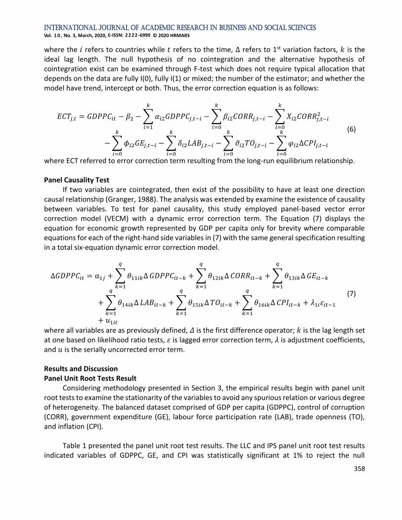
Table 4, it exhibits the average performance of GDP per capita and control of corruption of ASEAN countries from 1996 to 2018. The overall average performance of ASEAN countries in controlling corruption is above the threshold (2.23>1.84), but there is 4 out of 10 individual countries comprised of Indonesia (1.75), Laos (1.49), Cambodia (1.37), and Myanmar (1.20) are scoring below the threshold value of 1.84. Meanwhile, the threshold of 1.84 in controlling corruption also implies corruption levels of ASEAN countries at which to be reduced can be started at the very beginning by intensifying control of corruption.

Table 3: Panel ARDL Test Results based on PMG Estimator

Dependent variable (GDPPC) Panel ARDL/PMG

(1) (2)

CORR -1.247 (0.000) *** -2.025 (0.000) *** CORR2 - 1.662 (0.000) *** GE 0.677 (0.000) *** 0.247 (0.000) *** LAB -0.564 (0.000) *** 0.409 (0.000) *** TO 0.617 (0.000) *** 0.625(0.000) *** CPI -0.725 (0.000) *** 0.351 (0.000) *** ECT -0.028 (0.039) ** -0.038 (0.080) *

Threshold Control of Corruption 1.839

Notes: Values in parentheses denotes probability value. Asterisks ***, **, and * denote significance level at 1%, 5%, and 10%, respectively.



362

Table 4: Average of GDP per capita and Control of Corruption of ASEAN countries from 1996 to 2018

No. ASEAN Countries GDP per capita (constant 2010 US$ dollar)

Control of Corruption

1. Singapore 42880.22 4.66 2. Brunei 35343.85 3.01 3. Malaysia 8685.82 2.74 4. Thailand 4642.13 2.18 5. Philippines 2043.93 1.96 6. Vietnam 1180.49 1.94 7. Indonesia 2927.82 1.75 8. Laos 1043.77 1.49 9. Cambodia 706.01 1.37 10 Myanmar 795.86 1.20

Total Average Value 10024.99 2.23

Sources: Adapted and modified from Worldwide Governance Indicators (WGI) and World Development Indicators (WDI) published by World Bank. Panel Causality Test Results

Once the long run estimations have been determined. The next steps proceed to the panel Granger causality test to examine the causality between variables. Table 5 depicts the panel causality results examined by employing VECM Granger causality in a vector autoregression (VAR) system for ASEAN countries. Begins with the short-run causality results, it revealed there is a unidirectional short-run causality running from economic growth (GDPPC) to inflation (CPI), from GDPPC to government expenditure (GE), from control of corruption (CORR) to CPI, and from CPI to GE. Interestingly, there is absence of any short run causality with labour force participation rate. Figure 4 illustrated the direction of causality based on the panel causality test results presented in Table 5. By referring to Figure 4, there is short-run bidirectional causality running between GDPPC and TO, CORR and GE, CORR and TO, TO and GE. Also, there is indirect causality running between GDPPC and CORR, from GE to CPI, from GE to GDPPC as well as from CPI to CORR.

Meanwhile, in term of long-run dynamics based on the error correction terms estimated,

GDPPC, TO, and CPI each responds to deviations from long-run equilibrium given the negatively significant of respective ECT. Hence, it implies there is unidirectional long-run causality running from CORR, GE, LAB, TO, and CPI to economic growth with an estimated speed of adjustment towards long-run equilibrium of 0.010 (approximately 100 years to adjust towards equilibrium). Besides that, GDPPC, CORR, GE, LAB, and CPI jointly unidirectional causes trade openness in the long run with an



363

estimated speed of adjustment toward long-run equilibrium of 0.026 (approximately 38.5 years to adjust towards equilibrium). A long-run unidirectional causality was detected running from GDPPC, CORR, GE, LAB, and TO towards inflation with an estimated speed of adjustment of 0.015 (approximately 66.7 years to adjust toward equilibrium). It at the meantime implied ASEAN countries are vulnerable subject to any variations since there is requires for more than 35 years to one century for economic growth, trade openness, and inflation adjust back to long-run equilibrium after the shock.

Table 5: Panel Granger Causality Test Results

Dependent variables

𝚫GDPPC ΔCORR ΔGE ΔLAB ΔTO ΔCPI ECT

𝝌𝟐-statistics (p-value) Coefficient

ΔGDPPC - 3.277 (0.194)

1.405 (0.496)

2.389 (0.303)

8.879 (0.012)

**

0.228 (0.892)

-0.010 (0.000)

*** ΔCORR 0.257

(0.879) - 8.765

(0.013) **

1.980 (0.372)

5.501 (0.064) *

3.699 (0.157)

0.019 (0.000)

ΔGE 5.227 (0.073) *

9.115 (0.011) **

- 2.193 (0.334)

5.162 (0.076) *

9.973 (0.007)

***

0.009 (0.227)

ΔLAB 0.317 (0.853)

0.129 (0.938)

0.128 (0.938)

- 0.917 (0.632)

0.342 (0.843)

0.000 (0.318)

ΔTO 18.452 (0.000)

***

14.842 (0.001)

***

4.862 (0.088) *

3.862 (0.145)

- 55.864 (0.000)

***

-0.026 (0.000)

*** ΔCPI 6.036

(0.049) ** 5.587

(0.061) * 4.129

(0.127) 1.280

(0.527) 12.803 (0.002)

***

- -0.015 (0.001)

***

Notes: Parenthesized values are the probability of rejection of Granger non-causality. Δ is the first different operator. Asterisks ***, **, and * denote significance level at 1%, 5%, and 10%, respectively.



364

Unidirectional causality:

a) GDPPC CPI

b) GDPPC GE c) CORR CPI d) CPI GE Bidirectional causality: a) GDPPC TO b) CORR GE c) CORR TO d) TO GE Indirect causality: a) GDPPC CORR b) CORR GDPPC c) GE CPI d) GE GDPPC e) CPI CORR

Figure 4: Direction of Causality Conclusion and Policy Recommendation

This study examined the nexus between corruption and economic growth in ASEAN countries covering the period from 1996 to 2018. A panel data framework based on the panel unit root, panel cointegration and panel ARDL estimations, as well as panel Granger causality, was applied for the analysis in this study. The panel unit root test results denoted a mixed result as the variables integrated at I (0) and I (1). The Pedroni cointegration test results show there is significant cointegration among variables for ASEAN countries. The PMG estimator based on panel ARDL model revealed control of corruption reduce economic growth at the initial level, and after reaching the threshold, it starts conducive to the economic growth of ASEAN countries. Consequently, as nation achieves a lower level of corruption and promotes sustainable growth, whereby this U-shaped relationship between control of corruption and economic growth requires a threshold for over 1.84

CPI

GE GDPPC

TO

CORR



365

(control of corruption). It also revealed the level at which corruption is gradually reduced while promotes growth for ASEAN countries can be started at the very beginning. Although most of the ASEAN countries achieve governance in control of corruption above the estimated threshold of 1.84 but is still far from enough to achieve a better governance performance towards the lowest corruption level. The granger causality test result revealed the causality between control of corruption and other variables are mutually complementary. This reflecting a situation where prevalent corruption can exist at all level, at least in major economic activities, but if enhances governance in control of corruption also can affect those aspects through respective close linkage. Overall results provide evidence of both sand the wheels and grease the wheels' hypothesis.

Besides that, ASEAN countries should enhance the monitoring mechanism on the labour force

market since the impact of labour force participation rate only bring benign effect to economic growth when the corruption level is under controlled. A low level of controlling corruption can cause any possible deadweight loss or diminishing return of productivity of the labour force as the unproductive worker or human capital employed to engage in rent-seeking activities instead of productive activities. Besides that, ASEAN countries required to promote the efficiency and effectiveness of enforcement units to scrutinize prices of goods and services to prevent any party from driving up prices. Weak governance in controlling corruption conducive to illegitimate deal and collusion between enforcement units and businesses or individuals that involved in manipulating the prices beyond the official ceiling price or flow of commodities. In addition, ASEAN countries can reach a consensus to crackdown corruption unswervingly through joint or collaborative efforts to promote transparency, accountable and effectiveness institutional either at the individual country level or regional level. Moreover, an inclusive reform extended to economic, political or institutional, judicial and legislative, executive power, government recruitment system and so forth. A formidable status of political, economic and social will mitigate the effects of any uncertainty that may be imposed on ASEAN countries at all levels. In addition, future studies are encouraged to incorporate financial or institutions variables while grouping ASEAN countries into specific classification such as government size, natural resources, governance dimensions and so forth. Also, by covering longer periods, non-linear relationships can be extended not only to quadratic functions but to include cubic functions to study the existence of "rebound effects of corruption" on economic growth or development.

References Abu, N., Karim, M. Z. A., & Aziz, M. I. A. (2015). Corruption, political instability and economic

development in the Economic Community of West African States (ECOWAS): Is there a causal relationship? Contemporary Economics, 9(1), 45-60.

Aidt, T., Dutta, J., & Sena, V. (2008). Governance regimes, corruption and growth: Theory and evidence. Journal of Comparative Economics, 36(2), 195-220.

Amin, M. (2016). Informal firms in Myanmar. Enterprise Surveys Country Note Series, No.33. Informality. World Bank Group. Retrieved from

http://documents.worldbank.org/curated/en/204971482736208631/pdf/111251-BRI-PUBLIC-Informality-33.pdf.

Ata, A. Y., & Arvas, M. A. (2011). Determinants of economic corruption: A cross- country data. International Journal of Business and Social Science, 2(13), 161-169.



366

Ayaydın, H., & Hayaloglu, P. (2014). The effect of corruption on firm growth: Evidence from firms in Turkey. Asian Economic and Financial Review, 4(5), 607-624.

Azam, M., & Emirullah, C. (2014). The role of governance in economic development: Evidence from some selected countries in Asia and the Pacific. International Journal of Social Economics, 41(12), 1265-1278.

Aziz, M. N., & Sundarasen, S. D. D. (2015). The impact of political regime and governance on ASEAN economic growth. Journal of Southeast Asian Economics, 32(3), 375-389.

Bai, J., & Perron, P. (2003). Computation and analysis of multiple structural change models. Journal of Applied Econometrics, 18(1), 1-22.

Bhargava, V. (2005). The cancer of corruption. World Bank Global Issues Seminar Series. Retrieved from

http://www.eisourcebook.org/cms/February%202016/The%20Cancer%20of%20Corruption.pdf Bhattacharjee, J., & Haldar, S. K. (2015). Economic growth in South Asia: Binding constraints for the

future. Journal of South Asian Development, 10(2), 230-249. Bildirici, M. E. (2014). Relationship between biomass energy and economic growth in transition

countries: Panel ARDL approach. Global Change Biology (GCB) Bioenergy, 6(6), 717-726. Bose, N., Capasso, S., & Murshid, A. P. (2008). Threshold effects of corruption: Theory and evidence.

World Development, 36(7), 1173-1191. Cieślik, A., & Goczek, L. (2018). Control of corruption, international investment, and economic:

Evidence from panel data. World Development, 103, 323-335. Corruption Eradication Commission (KPK). (2015). Preventing state losses in Indonesia’s forest sector:

An analysis of non-tax forest revenue collection and timber production administration. Directorate of Research and Development, Deputy for Prevention, Corruption Eradication Commission (KPK), Republic of Indonesia. Retrieved from https://acch.kpk.go.id/images/tema/litbang/pengkajian/pdf/Preventing-State-Losses-in-Indonesia-Forestry-Sector-KPK.pdf

D’Agostino, G. D., Dunne, J. P., & Pieroni, L. (2012). Corruption, military spending and growth. Defence and Peace Economics, 23(6), 591-604.

Drury, A. C., Krieckhaus, J., & Lusztig, M. (2006). Corruption, democracy, and economic growth. International Political Science Review, 27(2), 121-136.

Engle, R. F., & Granger, W. J. (1987). Co-integration and error correction: Representation, estimation, and testing. Econometrica, 55(2), 251-276.

Enterprise Surveys. (2019). Corruption: East Asia & Pacific. The World Bank. Retrieved from https://www.enterprisesurveys.org/data/exploretopics/corruption#east-asia-pacific

GAN Integrity. (2016). Laos corruption report. GAN Business Anti-Corruption Portal. Retrieved from https://www.business-anti-corruption.com/country-profiles/laos/

GAN Integrity. (2017a). The Philippines corruption report. GAN Business Anti-Corruption Portal. Retrieved from https://www.business-anti-corruption.com/country-profiles/the-philippines/

GAN Integrity. (2017b). Vietnam corruption report. Retrieved from https://www.business-anti-corruption.com/country-profiles/vietnam/

Ghalwash, T. (2014). Corruption and economic growth: Evidence from Egypt. Modern Economy, 5(10), 1001-1009.



367

Granger, C. W. J. (1988). Some recent developments in a concept of causality. Journal of Econometrics, 39, 199-211.

Gregory, R. (2016). Combating corruption in Vietnam: A commentary. Asian Education and Development Studies, 5(2), 227-243.

Hashim, N. (2017). Development efforts and public sector corruption in Malaysia: Issues and challenges. Journal of Sustainability Science and Management, 12(2), 253-261.

Heckelman, J. C., & Powell, B. (2010). Corruption and the institutional environmental for growth. Comparative Economic Studies, 52(3), 351-378.

Huang, C. J. (2012). Corruption, economic growth, and income inequality: Evidence from ten countries in Asia. International Journal of Economics and Management Engineering, 6(6), 1141-1145.

Im, K. S., Pesaran, M. H., & Shin, Y. C. (2003). Testing for unit roots in heterogeneous panels. Journal of Econometrics, 115, 53-74.

Jayaraman, T. K., & Lau, E. P. H. (2009). Does external debt lead to economic growth in Pacific island countries. Journal of Policy Modeling, 31(2), 272-288.

Johnston, M. (1986). The political consequences of corruption: A reassessment. Comparative Politics, 18(4), 459-477.

Kennedy, S. (1997). Comrade’s dilemma: Corruption and growth in transition economies. Problems of Post-Communism, 44(2), 28-36.

Khaing, S. S. (2015). Tackling Myanmar’s corruption challenge. Munich Personal RePEc Archive (MPRA) Paper, No. 63764.

Kisswani, K. M. (2017). Evaluating the GDP-energy consumption nexus for the ASEAN-5 countries using nonlinear ARDL model. OPEC Energy Review, 41(4), 318-343.

Levin, A., Lin, C. F., & Chu, J. C. S. (2002). Unit root tests in panel data: Asymptotic and finite-sample properties. Journal of Econometrics, 108(1), 1-24.

Linhartova, V., & Zidova, E. (2016). Corruption as an obstacle to economic growth of national economies. Paper presented at the 18th International Scientific Conference on Economic and Social Development, Zagreb, Croatia.

Mallik, G., & Saha, S. (2016). Corruption and growth: A complex relationship. International Journal of Development Issues, 15(2), 113-129.

Mauro, P. (1995). Corruption and growth. The Quarterly Journal of Economics, 110(3), 681-712. Méndez, F., & Sepúlveda, F. (2006). Corruption, growth and political regimes: Cross country evidence.

European Journal of Political Economy, 22(1), 82-98. Mendonça, H, F. D., & Baca, A. C. (2017). Relevance of corruption on the effect of public health

expenditure and taxation on economic growth. Applied Economics Letters, 25(12), 876-881. Méon, P. G., & Sekkat, K. (2005). Does corruption grease or sand the wheels of growth? Public Choice,

122, 69-97. Méon, P. G., & Weill, L. (2010). Is corruption and efficient grease? World Development, 38(3), 244-

259. Mo, P. H. (2001). Corruption and economic growth. Journal of Comparative Economics, 29, 66-79. Okada, K., & Samreth, S. (2014). How does corruption influence the effect of foreign direct

investment on economic growth? Global Economic Review: Perspectives on East Asian Economies and Industries, 43(3), 207-220.



368

Ondo, A. (2017). Corruption and economic growth: The case of EMCCA. Theoretical Economics Letters, 7(5), 1292-1305.

Papaconstantinou, P., Tsagkanos, A. G., & Siriopoulos, C. (2013). How bureaucracy and corruption affect economic growth and convergence in the European Union: The case of Greece. Managerial Finance, 39(9), 837-847.

Paul, B. P. (2010). Does corruption foster growth in Bangladesh? International Journal of Development Issues, 9(3), 246-262.

Pesaran, M. H., & Shin, Y. C. (1999). An autoregressive distributed lag modelling approach to cointegration analysis. In Steinar, S (Ed.), Econometrics and economic theory in the 20th century: The Ragnar Frisch Centennial Symposium (pp. 371-413). Cambridge, United Kingdom: Cambridge University Press.

Pesaran, M. H., Shin, Y. C., & Smith, R. P. (1999). Pooled mean group estimation of dynamic heterogeneous panels. Journal of the American Statistical Association, 94(446), 621-634.

Pesaran, M. H., Shin, Y. C., & Smith R. J. (2001). Bound testing approaches to the analysis of level relationships. Journal of Applied Econometrics, 16(3), 289-326.

Pesaran, M. H., & Smith, R. (1995). Estimating long-run relationships from dynamic heterogeneous panels. Journal of Econometrics, 68(1), 79-113.

Pedroni, P. (1999). Critical values for cointegration tests in heterogeneous panels with multiple regressors. Oxford Bulletin of Economics and Statistics, 61(Special Issue), 653-670.

Pedroni, P. (2004). Panel cointegration: Asymptotic and finite sample properties of pooled time series tests with an application to the PPP hypothesis. Econometric Theory, 20, 597-625.

Pring, C. (2017). People and corruption: Asia Pacific-Global Corruption Barometer. Berlin, Germany: Transparency International.

Public Service Department Malaysia. (2019). Status tindakan susulan laporan ketua audit negara tahun 2012-2018 (Dikemaskini sehingga 6 Disember 2019). Retrieved from https://docs.jpa.gov.my/docs/pelbagai/2019/LKAN_06122019.pdf

Pulok, M. H., & Ahmed, M. U. (2017). Does corruption matter for economic development? Long run evidence from Bangladesh. International Journal of Social Economics, 44(3), 350-361.

Saha, S., & Ben Ali, M. S. (2017). Corruption and economic development: New evidence from the Middle Eastern and North African countries. Economic Analysis and Policy, 54, 83-95.

Saha, S., & Gounder, R. (2013). Corruption and economic development nexus: Variations across income levels in a non-linear framework. Economic Modelling, 31, 70-79.

Saha, S., & Yap, G. (2015), Corruption and tourism: An empirical investigation in a non-linear framework. International Journal of Tourism Research, 17(3), 272-281.

Stokke, K., Vakulchuk, R., & Øverland, I. (2018). Myanmar: A political economy analysis. Report commissioned by the Norwegian Ministry of Foreign Affairs. Oslo, Norway: Norwegian Institute of International Affairs.

Swaleheen, M. (2011). Economic growth with endogenous corruption: An empirical study. Public Choice, 146, 23-41.

The ASEAN Secretariat. (2017a). ASEAN economic integration brief. No.01/ June 2017. Jakarta, Indonesia. The ASEAN Secretariat.

The ASEAN Secretariat. (2017b). A journey towards regional economic integration: 1967-2017. Jakarta, Indonesia: The ASEAN Secretariat.



369

The ASEAN Secretariat. (2019). ASEAN economic integration brief. No.06/ November 2019. ASEAN Integration Monitoring Directorate (AIMD) and Community Relations Division (CRD). Jakarta, Indonesia: The ASEAN Secretariat.

The World Bank. (2018). Combating Corruption. Retrieved from http://www.worldbank.org/en/topic/governance/brief/anti-corruption

Tomaszewski, M. (2018). Corruption: A dark side of entrepreneurship, corruption and innovations. Prague Economic Papers, 27(3), 251-269.

Transparency International. (2015). ASEAN integrity community: A vision for transparent and accountable integration. Berlin, Germany: Transparency International.

Transparency International. (2018). What is corruption? Retrieved from https://www.transparency.org/what-is-corruption#define.

Transparency International Cambodia. (2014). Corruption and Cambodia’s governance system: The need for reform. Phnom Penh, Kingdom of Cambodia: Transparency International Cambodia.

Transparency International Secretariat. (2019, January 29). Corruption perceptions index 2018 shows anti-corruption efforts stalled in most countries: Analysis reveals corruption contributing to a global crisis of democracy. Transparency International. Retrieved from

https://www.transparency.org/news/pressrelease/corruption_perceptions_index_2018. United Nations. (n.d.). Sustainable development goals. Retrieved from

https://sustainabledevelopment.un.org/sdgs United Nations Office and Drugs and Crime (UNODC). (2019). UNODC and the sustainable

development goals. Retrieved from https://www.unodc.org/documents/SDGs/UNODC-SDG_brochure_LORES.pdf.

Wang, Y. Y., & You, J. (2012). Corruption and firm growth.: Evidence from China. China Economic Review, 23(2), 415-433.

corruption and growth in asean countries: a non-linear

Documents