cosmocalc: an excel add-in for cosmogenic nuclide...

CosmoCalc: An Excel add-in for cosmogenic nuclidecalculations

Pieter VermeeschInstitute of Isotope Geology and Mineral Resources, ETH-Zurich, Clausiusstrasse 25, NW C85, CH-8092, Zurich,Switzerland ([email protected])

[1] As dating methods using Terrestrial Cosmogenic Nuclides (TCN) become more popular, the need arisesfor a general-purpose and easy-to-use data reduction software. The CosmoCalc Excel add-in calculatesTCN production rate scaling factors (using Lal, Stone, Dunai, and Desilets methods); topographic, snow,and self-shielding factors; and exposure ages, erosion rates, and burial ages and visualizes the results onbanana-style plots. It uses an internally consistent TCN production equation that is based on the quadrupleexponential approach of Granger and Smith (2000). CosmoCalc was designed to be as user-friendly aspossible. Although the user interface is extremely simple, the program is also very flexible, and nearly alldefault parameter values can be changed. To facilitate the comparison of different scaling factors, a set ofconverter tools is provided, allowing the user to easily convert cut-off rigidities to magnetic inclinations,elevations to atmospheric depths, and so forth. Because it is important to use a consistent set of scalingfactors for the sample measurements and the production rate calibration sites, CosmoCalc defines theproduction rates implicitly, as a function of the original TCN concentrations of the calibration site. Theprogram is best suited for 10Be, 26Al, 3He, and 21Ne calculations, although basic functionality for 36Cl and14C is also provided. CosmoCalc can be downloaded along with a set of test data from http://cosmocalc.googlepages.com.

Components: 5243 words, 4 figures, 1 table.

Keywords: cosmogenic nuclides; Excel; exposure dating; banana plots; calculator.

Index Terms: 1150 Geochronology: Cosmogenic-nuclide exposure dating (4918); 1105 Geochronology: Quaternary

geochronology; 1194 Geochronology: Instruments and techniques.

Received 16 November 2006; Revised 7 February 2007; Accepted 1 May 2007; Published 9 August 2007.

Vermeesch, P. (2007), CosmoCalc: An Excel add-in for cosmogenic nuclide calculations, Geochem. Geophys. Geosyst., 8,

Q08003, doi:10.1029/2006GC001530.

1. Introduction

[2] The first applications of Terrestrial CosmogenicNuclide (TCN) geochronology appeared about20 years ago [Kurz, 1986; Nishiizumi et al.,1986; Phillips et al., 1986]. The method hasrapidly developed since those early days, trulyrevolutionizing geomorphology and related fields

in the process. TCN dating is no longer a special-ized tool used by a small group of experiencedusers, but has found an ever growing base of userswho are not necessarily familiar with all the detailsof the method. Today we are facing a paradoxicalsituation. On the one hand, a better understandingof cosmogenic nuclide production systematics hasimproved the accuracy of TCN dating. But on theother hand, many users of the method may be less

G3G3GeochemistryGeophysics

Geosystems

Published by AGU and the Geochemical Society

AN ELECTRONIC JOURNAL OF THE EARTH SCIENCES

GeochemistryGeophysics

Geosystems

Article

Volume 8, Number 8

9 August 2007

Q08003, doi:10.1029/2006GC001530

ISSN: 1525-2027

ClickHere

for

FullArticle

Copyright 2007 by the American Geophysical Union 1 of 14

http://dx.doi.org/10.1029/2006GC001530

familiar with its intricacies than was the case in thepioneering days. An important example of thissituation is that of the production rate scalingfactors. In a landmark paper, Lal [1991] presenteda method to calculate cosmogenic nuclide produc-tion rates as a function of latitude and elevation.Lal’s scaling factors are elegant and easy to use,but overestimate the importance of muons and areonly valid for standard atmosphere. Later authorsintroduced several improvements, incorporatingatmospheric effects and improved muon produc-tion systematics. The scaling factors of Stone[2000], Dunai [2000], Desilets and Zreda [2003],and Desilets et al. [2006] more accurately representthe scaling of cosmogenic nuclide production rateswith latitude and elevation, but the increased so-phistication of these methods is an obstacle to theirwidespread use.

[3] CosmoCalc is an add-in to MS-Excel devel-oped with the intention to alleviate this problem.The CosmoCalc interface was designed to be asuser friendly and easy-to-use as possible. Defaultparameters are set so that beginning users onlyhave to make a minimal number of decisions. Atthe same time, all the default parameters can bechanged so that CosmoCalc is highly customizableand also experienced users should find it useful.The program as well as a spreadsheet with test datacan be downloaded from the CosmoCalc Web sitehttp://cosmocalc.googlepages.com), which alsoprovides detailed installation instructions. Theadd-in requires MS-Excel 2000 or higher. Becauseof small differences between the MS-Windows andApple OS-X implementations of Excel, two ver-sions of CosmoCalc are provided. The functional-ity of both programs is the same, but the Macintoshversion is significantly slower than the PC version.

[4] After installing the CosmoCalc add-in, a tool-bar menu appears (Figure 1) that guides the userthrough the data reduction and closely follows theoutline of this paper:

. Production rate scaling factors (section 2)–Lal [1991]–Stone [2000]–Dunai [2000]–Desilets and Zreda [2003]–Desilets et al. [2006]

. Shielding corrections (section 3)–Topographic shielding–Self shielding–Snow shielding

. Banana plots (section 4)–26Al-10Be–21Ne-10Be

. Age-erosion rate calculations (section 5)–Single nuclide: exposure age and erosion

rate calculations for 26Al, 10Be, 21Ne, 3He, 36Cland 14C

–Two nuclides: simultaneous calculation of(burial or exposure) age and erosion rate.

. Converters (section 6)–Convert elevation to atmospheric pressure or

-depth and back, under standard and Antarcticatmosphere.

–Convert geomagnetic latitude to -inclinationor cutoff rigidity and back.

. Settings: customizing CosmoCalc (section 7)–Specify TCN production rate calibration

sites–Specify the relative importance of various

production pathways

[5] The following sections will provide more detailsabout these calculations. Thus the present paperserves as an abridged review of TCN calculations,with an emphasis on the numerical methods that areneeded to solve the equations. More details about thephysics of TCN production are given in the reviewarticle of Gosse and Phillips [2001]. CosmoCalc isnot the first computational tool for TCN calculations.Useful alternatives are CHLOE, anExcel spreadsheetfor cosmogenic 36Cl calculations [Phillips andPlummer, 1996] and the CRONUS-Earth Webcalculator (http://hess.ess.washington.edu/math)(G. Balco and J. O. H. Stone, A simple, internallyconsistent, and easily accessible means of calculat-ing surface exposure ages or erosion rates from10Be and 26Al measurements, manuscript inpreparation, 2007; hereinafter referred to as Balcoand Stone, manuscript in preparation, 2007).CosmoCalc was developed independently fromthese other tools, except for its topographicshielding correction function, which was translatedinto VBA from the Matlab code of Balco andStone (manuscript in preparation, 2007). Thereader is strongly encouraged to try these otherprograms. CosmoCalc is optimized for 26Al, 10Be,21Ne and 3He dating. Because geomagnetic fieldfluctuations and thermal neutron reactions areignored, results for 36Cl and 14C may be inaccurate.CosmoCalc can be used as an exploratory tool forthese nuclides, but for more accurate results,CHLOE and the spreadsheet of Lifton et al.[2005] are recommended.

2. Production Rate Scaling Factors

[6] In the simplest case (no shielding or burial),only three pieces of information are needed to

GeochemistryGeophysicsGeosystems G3G3

vermeesch: cosmocalc: an excel add-in 10.1029/2006GC001530

2 of 14

calculate an exposure age or erosion rate: TCNconcentration, half-life and production rate. Pro-duction rates are the ‘‘Achilles’ heel’’ of the TCNmethod. There exist only a few calibration siteswhere TCN production rates are accurately knownthanks to the availability of independent age con-straints [e.g., Nishiizumi et al., 1989; Niedermannet al., 1994; Kubik et al., 1998]. These productionrates are only valid for the specific conditions(latitude, elevation, age) of each particular calibra-tion site. To apply the TCN method to other fieldsettings, the production rates must be scaled to acommon reference at sea level and high latitude(SLHL). Up to 20% uncertainty is associated withthis scaling, constituting the bulk of TCN ageuncertainty.

[7] Although several efforts have been made todirectly measure TCN production rate scaling withlatitude and elevation using artificial H2O and SiO2

targets [Nishiizumi et al., 1996; Brown et al., 2000;I. J. Graham et al., Direct measurement of cosmo-genic production of 7Be and 10Be in water targetsin the southern hemisphere, manuscript in prepara-tion, 2007], all currently used scaling models arebased on neutron monitor surveys. The oldest andstill most widely used scaling model is that of Lal[1991]. This model is a simple set of polynomialequations giving the (spallogenic + muogenic)production rate relative to SLHL as a function ofgeographic latitude and elevation. In CosmoCalc,Lal’s scaling factors can be calculated by simplyselecting two columns of latitude (in degrees) andelevation (in meters) data and clicking ‘‘OK’’.

[8] Lal’s scaling factors use elevation as a proxyfor atmospheric depth, assuming a standard atmo-sphere approximation. Stone [2000] noted that this

approximation is not valid in certain areas, such asAntarctica and Iceland. To avoid the systematicerrors caused by the standard atmosphere model,Stone [2000] recast the polynomial equations ofLal [1991] in terms of air pressure instead ofelevation. A second improvement of the Stone[2000] model is the independent scaling of TCNproduction by slow (negative) muons [Heisinger etal., 2002a, 2002b]. In spite of this added complex-ity, the CosmoCalc interface for Stone [2000]scaling factors is identical to that for Lal [1991]scaling: the user simply needs to provide twocolumns of data, one with latitude and one withair pressure (in mbar). The scaling factors of Stone[2000] can be different for different nuclides,because the importance of muons depends on thenuclide of interest. Because most TCN productionrate calibration sites are not located at SLHL, it iscrucially important to scale the production ratesusing the same method as the unknown sample.This is exactly what CosmoCalc does when theuser selects a nuclide from the scroll-down menu ofthe scaling-form. Thus the program ‘‘forces’’ theuser to be consistent. The program comes with aset of default calibration sites, but these can bechanged. Also the relative importance of the pro-duction pathways (neutrons, slow and fast muons)can be changed (section 7).

[9] Behind the scaling models of both Lal [1991]and Stone [2000] lies an extensive database ofneutron monitor measurements, ordered accordingto geomagnetic latitude. This ordering implies thatEarth’s magnetic field can be accurately approxi-mated by a simple dipole. To avoid this approxi-mation, Dunai [2000] ordered the neutron monitordata according to geomagnetic inclination, whichalso represents the non-dipole field. Just like Stone[2000], Dunai [2000] also incorporates separatemuon scaling and atmospheric effects. However,atmospheric depth (g/cm2) is used instead of airpressure. Using CosmoCalc it is very easy toconvert air pressure to elevation or atmosphericdepth and back (section 6).

[10] Ultimately, both geomagnetic latitude and in-clination are merely proxies for a more fundamen-tal physical quantity: the geomagnetic cutoffrigidity (Rc), which is the minimum momentumper unit charge (in GV), required for a primarycosmic ray to reach the atmosphere. Ordering theneutron monitor data according to this parameterresults in yet another set of scaling factors. Unfor-tunately, at least three different methods for calcu-lating Rc exist in the literature. Dunai [2001] used a

Figure 1. CosmoCalc’s main menu guides the userthrough the data reduction and follows the outline ofthis paper.


vermeesch: cosmocalc: an excel add-in 10.1029/2006GC001530vermeesch: cosmocalc: an excel add-in 10.1029/2006GC001530

3 of 14

database of horizontal magnetic field intensitiesand inclinations to estimate the cutoff-rigidity ofan equivalent axial dipole field, for which anapproximate analytical solution exists. Desiletsand Zreda [2003] used a model based on trajectorytracing of an axial dipole field, which is done bynumerically testing the feasibility of verticallyincident anti-protons to travel from the top of theatmosphere back into space. Finally, Lifton et al.[2005] fit a cosine function to a database ofgeomagnetic latitudes versus trajectory traced cut-off rigidities for the 1955 magnetic field. Theseauthors consider the scatter around their fit to be arealistic estimator of the natural variability of Rc atany given geomagnetic latitude.

[11] In order to avoid confusion, CosmoCalc cur-rently only implements one of these three methods,namely that of Desilets and Zreda [2003]. Thescaling model of Desilets and Zreda [2003] makesa distinction between slow and fast muons, each ofwhich scales differently. In an update of theirmodel, Desilets et al. [2006] did a neutron monitorsurvey at low latitudes, which were undersampledby previous surveys. This resulted in a slightlydifferent set of attenuation length polynomials forspallogenic reactions. The method of Desilets andZreda [2003] and Desilets et al. [2006] is probablythe most accurate of all the scaling models imple-mented in CosmoCalc. It is also the most complexmodel, but this did not change the user interface.Using the scaling models of Desilets and Zreda[2003] and Desilets et al. [2006] is just as easy asthat of Lal [1991] in CosmoCalc. Default valuesfor the relative SLHL production rate contributionsof neutrons, slow and fast muons can be changed inthe Settings menu (section 7).

[12] The scaling models of Dunai [2001], Desiletsand Zreda [2003], Desilets et al. [2006], Pigati andLifton [2004], and Lifton et al. [2005] are asensitive function of magnetic field intensity andsolar activity, both of which are poorly constrainedover geologic time. On the one hand, this temporalvariability is the biggest downside to Rc-basedmodels for long exposures (>20 ka [Dunai,2001]). On the other hand, such models also offerthe possibility to correct for secular variation ofTCN production rates for short exposures. Instruc-tions for doing so are given by Dunai [2001] andDesilets and Zreda [2003], provided a local recordof paleomagnetic intensity is available. Compilingsuch a record is something for advanced users andfalls beyond the scope of CosmoCalc. The scalingmodels of Pigati and Lifton [2004] and Lifton et al.

[2005] are accompanied by global data sets ofmagnetic field intensity, polar wander and solaractivity and in principle, it would have been possibleto incorporate these data sets into CosmoCalc.However, because they are very large (4 and 7 Mb,respectively) in comparison with CosmoCalc itself(�500 kb), the cost of including these scalingmodels was considered too high. Thereforeresearchers working with 14C, where secular varia-tion of the magnetic field is really crucial, should useCosmoCalc only as an exploratory tool, and use thespreadsheets of Pigati and Lifton [2004] and Liftonet al. [2005] for final calculations.

3. Shielding Corrections

[13] The scaling factors discussed in the previoussection allow the calculation of TCN productionrates at any location on the Earth’s surface, assum-ing that the sample is a slab of zero thickness takenfrom a horizontal planar surface. If these assump-tion are not fulfilled, the SLHL production ratesmust be multiplied by a second set of correctionfactors, quantifying the extent to which the cosmicrays were blocked. CosmoCalc implements threesuch correction factors: topographic shielding, selfshielding and snow cover.

3.1. Topographic Shielding

[14] Two kinds of topographic shielding correc-tions can be distinguished for (1) samples takenfrom a tilted rather than horizontal surface and(2) samples that are located in the vicinity oftopographic irregularities. CosmoCalc follows theapproach of Balco and Stone (manuscript in prep-aration, 2007) (their Matlab function skyline.m)and treats these two effects together using thefollowing equation:

St ¼ 1�Z 2p

0

sin h qð Þð Þ3:5

2pdq ð1Þ

[15] With h(q) the ‘‘horizon’’ in the azimuthaldirection q, i.e., either the elevation (in radians)of the topography or the sloping sample surface,whichever is greatest. Sometimes, an exponent of2.3 is used instead of 3.5 in equation (1) [Staudacherand Allegre, 1993]. CosmoCalc treats this expo-nent as a variable, which can be changed in theSettings form (section 7). In practice, the integralof equation (1) is solved by linear interpolationbetween a finite number of azimuth/elevationmeasurements. The input needed by CosmoCalcis two mandatory columns of strike and dip (in



4 of 14

degrees, where the strike is 90 degrees less than thedirection of the dip), followed by an optional seriesof topographic azimuth/elevation measurements (indegrees). There is no restriction on the total numberof measurements, provided they come in multiplesof two.

3.2. Self-Shielding

[16] Cosmic rays are rapidly attenuated as theytravel through matter, causing TCN productionrates to vary greatly with depth below the rock/air contact. They must be integrated over the actualsample thickness and scaled to the surface produc-tion rates before an exposure age can be calculated.Different reaction mechanisms are associated withdifferent attenuation lengths. Gosse and Phillips[2001] consider four kinds of thickness corrections,for spallogenic, thermal and epithermal neutrons,and muons. Because self-shielding corrections aregenerally small, CosmoCalc considers only thespallogenic neutron reactions:

Ss ¼L0

rz1� e

� rzL0

� �ð2Þ

with L0 the spallogenic neutron attenuation length(default value 160 g/cm2), r the rock density(default value 2.65 g/cm3) and z the samplethickness (in cm). Neglecting the remaining path-ways makes little difference, with the possibleexception of 36Cl, because the latter can bestrongly affected by thermal neutron fluxes, whichare currently ignored by CosmoCalc.

3.3. Snow Cover

[17] Perhaps the most popular and powerful appli-cation of TCN techniques is the dating of glacialmoraines [e.g., Gosse et al., 1995; Schafer et al.,1999]. These features are generally located at highlatitudes or elevations, where snow cover poses apotential problem. The snow correction is similarto the self-shielding correction with the importantdifference that the former is highly variable withtime. Given n (e.g., 12 for monthly or 4 forseasonal) measurements of average snow thicknessz and density r, CosmoCalc computes the snowcorrection factor Sc as follows:

Sc ¼1

n

Xni¼1

e�r ið Þz ið Þ

L0 ð3Þ

4. Banana Plots

[18] Before calculating an exposure age or erosionrate, it is a good idea to check if the TCN measure-

ments are consistent with a simple or complexexposure history. This can be done with twonuclides (including at least one radionuclide) usinga ‘‘banana plot’’ [Lal, 1991]. CosmoCalc accom-modates two types of banana plot: 26Al-10Be and21Ne-10Be. Depending on whether or not a sampleplots above, below or inside the so-called ‘‘steady-state erosion island’’ [Lal, 1991], one can decidewhether or not to pursue the calculation of anexposure age, erosion rate or burial age. For theconstruction of the banana plots and the age-erosion calculations of section 5, CosmoCalcimplements a modified version of the ingrowthequation of Granger and Muzikar [2001]:

N ¼ Pe�ltX3i¼0

Fi

lþ �r=Li

1� e� lþ�r=Lið Þt� �

ð4Þ

[19] With N the nuclide concentration (atoms/g),P the total surface production rate (in atoms/g/yr) atSLHL, t the burial age, � the erosion rate, t theexposure age and l the radioactive half-life of thenuclide. Equation (4) models TCN production byneutrons, slow and fast muons by a series ofexponential approximations. The first term of thesummation models TCN production by spallogenicneutron reactions, the second and third termsmodel slow muons and the last term approximatesTCN production by fast muons. Thus F0,. . ., F3

are dimensionless numbers between zero and one,and L0,. . ., L3 are attenuation lengths (g/cm2).The approach of Granger and Smith [2000] andGranger et al. [2001] was chosen because of itsflexibility. For instance, neglecting muon produc-tion can be easily implemented by setting F1, F2

and F3 equal to zero in equation (4). CosmoCalcuses Granger and Smith’s [2000] and Granger etal.’s [2001] recommended values of F0,. . ., F3 for10Be and 26Al, but also offers an alternative choiceof pre-set values approximating either the alterna-tive parameterization of Schaller et al. [2002],neglecting the contribution of muons, or only usingthree exponentials (for more details, see section 7).Banana plots with non-zero muon contributionsfeature a characteristic cross-over of the steady-state and zero erosion lines which is absent whenmuons are neglected (Figure 2).

[20] CosmoCalc’s banana plots are normalized toSLHL, meaning that the TCN concentrations ofeach sample are divided by the cumulative effect ofall their correction factors, represented by the‘‘effective scaling factor’’ Se:

Se ¼ St � f Sð Þ ð5Þ



5 of 14

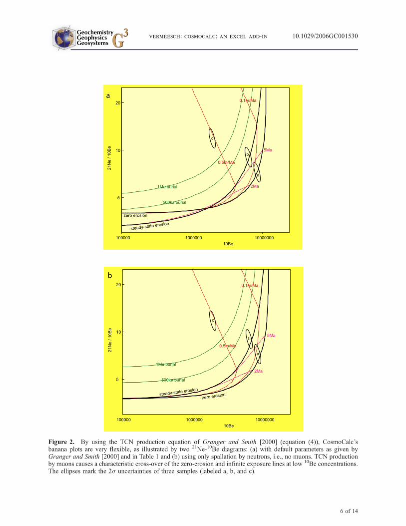
Figure 2. By using the TCN production equation of Granger and Smith [2000] (equation (4)), CosmoCalc’sbanana plots are very flexible, as illustrated by two 21Ne-10Be diagrams: (a) with default parameters as given byGranger and Smith [2000] and in Table 1 and (b) using only spallation by neutrons, i.e., no muons. TCN productionby muons causes a characteristic cross-over of the zero-erosion and infinite exposure lines at low 10Be concentrations.The ellipses mark the 2s uncertainties of three samples (labeled a, b, and c).



6 of 14

with

S ¼ Sp � Ss � Sc ð6Þ

where Sp is one of the production rate scalingfactors of section 2 and St, Ss and Sc are definedin section 3. If muon production is neglected, thenSe = St � Sp � Ss � Sc. However, in the presenceof muons, the effective scaling factor Se maydeviate from this value because the relativeimportance of the different production mechanismschanges as a function of age, erosion rate,elevation, latitude, sample thickness and snowcover. The exact form of the function f(S) will bedefined in section 5.2.4. Note that the topographicshielding correction St does not ‘‘fractionate’’ (i.e.,change the fractions F0,. . .,F3 of) the differentproduction mechanisms and is placed outside thescaling function f(S). This means that, strictlyspeaking, the TCN concentrations should bedivided by St prior to generating a banana plot.The input required by CosmoCalc’s ‘‘Banana’’function are (1) the composite scaling factor S forthe first nuclide (26Al or 21Ne), (2) the concentra-tion and 1s measurement uncertainty of the firstnuclide (26Al or 21Ne), both divided by St, (3) S forthe second nuclide (10Be), and (4) the concentra-tion and 1s measurement uncertainty of the secondnuclide (10Be), also divided by St. Becausetopographic shielding corrections are generallysmall, the systematic error caused by lumping Sttogether with the other correction factors is verysmall. Therefore, if St > �0.95, say, it is safe toapproximate equation (5) by Se = f(St � Sp � Ss �Sc). In this case, the nuclide concentrations do notneed to be pre-divided by St.

[21] The graphical output of CosmoCalc can easilybe copied and pasted for editing in vector graphicssoftware such as Adobe Illustrator or CorelDraw.The y-axis of the 26Al-10Be plot is logarithmic bydefault whereas the y-axis of the 21Ne-10Be plot islinear. These defaults can be changed in the‘‘Banana Options’’ userform. Note that MS-Excel(versions 2000 and 2003) only allows logarithmictick marks to have values in multiples of ten. To getaround this limitation, CosmoCalc uses a ‘‘pseudoy-axis’’, which cannot be edited by the usual rightmouse button click. Hopefully, this limitation willnot be necessary in later versions of Excel. Cos-moCalc only propagates the analytical uncertaintyof the measured TCN concentrations. No uncer-tainty is assigned to the production rate scalingfactors, radioactive half-lives or other potentiallyill-constrained quantities. On the banana plots,the user is offered the choice between error bars

or -ellipses with the latter being the default. Bananaplots are graphs of the type N1/N2 vs. N2 which arealways associated with some degree of ‘‘spuriouscorrelation’’ [Chayes, 1949]. This causes the errorellipses to be rotated according to the followingcorrelation coefficient:

rc ¼ ��N1sN2ffiffiffiffiffiffiffiffiffiffiffiffiffiffiffiffiffiffiffiffiffiffiffiffiffiffiffiffiffiffiffi

�N22s

2N1

þ �N21s

2N2

q ð7Þ

[22] If N1 stands for26Al or 21Ne and N2 for

10Be,then �N1 and �N2 are the measured concentrations ofthese respective nuclides while sN1 and sN2 are thecorresponding measurement uncertainties.

5. Age-Erosion Rate Calculations

[23] Equation (4) has three unknowns: t (exposureage), � (erosion rate) and t (burial age). If only onenuclide was measured, we must assume values fortwo of these quantities in order to solve for thethird. If two nuclides were analyzed (of which atleast one is radioactive), only one assumption isneeded. CosmoCalc is capable of both approaches.In this section, we will first discuss how to solvefor � (assuming infinite exposure age and zeroburial) and t (assuming zero erosion and burial)using a single nuclide (section 5.1). Then, numer-ical methods will be presented to simultaneouslysolve for t and � (assuming zero burial), t and t(assuming zero erosion) or � and t (assuming infiniteexposure age), using two nuclides (section 5.2). Notethat in the case of two nuclides (26Al or 21Necombined with 10Be), the assumption of zero burialcan be verified on the banana plot.

5.1. Calculations Using a Single Nuclide

[24] CosmoCalc requires three pieces of informa-tion to calculate an exposure age or erosion rate:the TCN concentration (corrected for topography),its analytical uncertainty and a composite correc-tion factor for production rate scaling with latitude/elevation and shielding (equation (6)). We some-how need to incorporate this scaling factor into theingrowth equation (equation (4)). This poses aproblem because the scaling factor is a singlenumber whereas equation (4) explicitly makesthe distinction between neutrons, slow and fastmuons. Granger and Smith [2000] avoid thisproblem by separately scaling the different pro-duction mechanisms:

N t; �; tð Þ ¼ Pe�ltX3i¼0

SiFi

lþ �r=Li

1� e� lþ�r=Lið Þt� �

ð8Þ



7 of 14

[25] Instead of one scaling factor, equation (8) hasfour, one for neutrons (S0), two for slow muons (S1and S2) and one for fast muons (S3). Granger et al.[2001] separately calculate each of these four scal-ing factors. Thus the original method of Grangerand Smith [2000] is incompatible with the commonpractice of lumping all production mechanisms intoa single latitude/elevation scaling factor (section 2).To ensure optimal flexibility and user-friendliness,CosmoCalc uses a slightly different approach.S0,. . ., S3 are calculated from the composite cor-rection factor S, by approximating the total scalingby a single attenuation factor caused by a virtuallayer of matter of thickness x (in g/cm2):

Si ¼ e�x=Li for i ¼ 0; . . . ; 3 ð9Þ

so that

X3i¼0

SiFi ¼ S ð10Þ

with Fi and Li as in equation (4) and S as defined inequation (6). CosmoCalc solves equation (10)iteratively using Newton’s method.

[26] As said before, some assumptions are neededto solve equation (8). An exposure age (t) can becalculated under the assumption of zero erosionand burial (� = 0, t = 0). For a radionuclide withdecay constant l, this yields:

t ¼ � 1

lln 1� Nl

PS

� �ð11Þ

whereas for stable nuclides (3He and 21Ne):

t ¼ N

PSð12Þ

[27] Alternatively, the erosion rate (�) can be cal-culated under the assumption of steady state andzero burial (t = 1, t = 0):

N �ð Þ ¼ PX3i¼0

SiFi

lþ �r=Li

ð13Þ

[28] CosmoCalc solves this equation iterativelyusing Newton’s method. Statistical uncertaintiesare estimated by standard error propagation:

st ¼sN

PS � Nlð14Þ

s� ¼sN

PP3

i¼0SiFi

Li=rð Þ lþ�r=Lið Þð Þ2ð15Þ

[29] These error estimates do not include anyuncertainties in production rates and scaling fac-tors, which are difficult to quantify, but can beevaluated by using a range of input parameters.

5.2. Calculations With Two Nuclides

[30] Equation (8) has three unknowns (t, � and t).If two nuclides have been measured (with concen-trations N1 and N2, say), only one value must beassumed in order to solve for the remaining two.By assuming zero erosion (� = 0), CosmoCalcsimultaneously calculates the exposure age andburial age (section 5.2.1); by assuming steady-stateerosion (t = 1), the erosion rate and burial age arecalculated; and by assuming zero-burial (t = 0), theerosion rate and exposure age can be computed(section 5.2.2).

5.2.1. Burial Dating

[31] If a rock surface gets buried by sediments orcovered by ice, it is shielded from cosmic rays andthe concentration of cosmogenic radionuclidesdecays with time. Such samples plot outside thesteady-state erosion island of the banana plot, inthe so-called field of ‘‘complex exposure’’, a fea-ture which is considered undesirable by moststudies. Other studies, however, intentionally targetcomplex exposure histories, using radionuclides todate pre-exposure and burial [e.g., Bierman et al.,1999; Fabel et al., 2002; Partridge et al., 2003].CosmoCalc calculates burial ages, either by assum-ing negligible erosion or steady state erosion (� = 0or t = 1, respectively). It does not handle post-depositional nuclide production.

5.2.1.1. Burial-Exposure Dating

[32] If � = 0, equation (8) reduces to:

N ¼ e�lt SP

l1� e�lt �

ð16Þ

[33] The easiest case of two-nuclide dating is thatof simultaneously calculating exposure age (t) andburial age (t) with one radionuclide and one stablenuclide. Because the stable nuclide is not affectedby burial, it can be used to calculate the pre-exposure age, using equation (12). This age canthen be used to calculate the burial age:

t ¼ 1

lln

SP

Nl1� e�lt ��

ð17Þ



8 of 14

[34] In the case of two radionuclides, CosmoCalcfinds t by iteratively solving the following equationusing Newton’s method:

l2 lnSPð Þ1N1l1

1� e�l1 t ��

� l1 lnSPð Þ2N2l2

1� e�l2 t ��

¼ 0

ð18Þ

[35] With l1> l2. The solution is then plugged intoequation (17), using nuclide 1.

5.2.1.2. Burial-Erosion Dating

[36] Setting t = 1 in equation (8) yields thefollowing system of non-linear equations forTCN concentrations N1 and N2:

f1 �; tð Þ : N1 ¼ P1e�l1t

P3i¼0

Si;1Fi;1

l1 þ �r=Li;1

f2 �; tð Þ : N2 ¼ P2e�l2t

P3i¼0

Si;2Fi;2

l2 þ �r=Li;2

8>><>>: ð19Þ

[37] These equations are easy to solve since thevariables t and � are separated. If nuclide 1 hasthe shortest half-life (largest decay constant l), theburial age is written as a function of the erosionrate �:

t ¼ 1

l1

lnP1

N1

X3i¼0

Si;1Fi;1

l1 þ �r=Li;1

!ð20Þ

[38] The erosion rate is given implicitly by:

l2 lnP1

N1

X3i¼0

Si;1Fi;1

l1 þ �r=Li;1

!

� l1 lnP2

N2

X3i¼0

Si;2Fi;2

l2 þ �r=Li;2

!

¼ 0 ð21Þ

[39] CosmoCalc solves equation (21) for � usingNewton’s method and then plugs this value intoequation (20). If l2 < l1, then N2 is used instead ofN1 in equation (20).

5.2.2. Age-Erosion Rate Calculations

[40] Assuming zero burial (t = 0) yields thefollowing system of equations f1 and f2:

f1 �; tð Þ : N1 ¼ P1

P3i¼0

Si;1Fi;1

l1 þ �r=Li;11� e� l1þ�r=Li;1ð Þt� �

f2 �; tð Þ : N2 ¼ P2

P3i¼0

Si;2Fi;2

l2 þ �r=Li;21� e� l2þ�r=Li;2ð Þt� �

8>><>>:

ð22Þ

[41] It is impossible to solve these equations forexposure age (t) and erosion rate (�) separately.Instead, CosmoCalc implements the two-dimensionalversion of the Newton-Raphson algorithm:

�kþ1

tkþ1

24

35 ¼

�k

tk

24

35�

a ¼ @f1@�

� �kb ¼ @f1

@t

� �k

c ¼ @f2@�

� �kd ¼ @f2

@t

� �k

264

375�1

f1 �k ; tkð Þ

f2 �k ; tkð Þ

24

35

ð23Þ

[42] With J(�, t) =a b

c d

� �the Jacobian matrix,

which is also used for error propagation.

5.2.3. Error Propagation

[43] Error propagation is less straightforward in thetwo-dimensional case than in the single nuclidecase (section 5.1). The bijection from (N1,N2)-space to (�,t)-space is not orthogonal, particularlyin the case of age-erosion dating (section 5.2.2).For this reason, it is only possible to analyticallycompute upper bounds for s(�), s(t) and s(t):

s xð Þ

s yð Þ

24

35 k J x; yð Þ�1k

s N1ð Þ

s N2ð Þ

24

35 ð24Þ

with x and y placeholders for � and t or t,respectively, And k�k the absolute values of thematrix [�]. In the case of age-erosion dating, theconfidence intervals for t and � are very wide, oftentoo wide to be useful. Therefore it can be moreproductive to solve each quantity separately insteadof simultaneously. Thus, using equations (11) and(13), it is possible to estimate minimum exposureages and maximum erosion rates [e.g., Nishiizumiet al., 1991]. However, for burial dating there is nochoice and we must simultaneously solve for t and

� or t.

[44] In addition to Newton’s method, CosmoCalcoffers a second way of solving equations (19)and (22) by means of Monte Carlo simulation,implementing the Metropolis-Hastings algorithm[Metropolis et al., 1953; Tarantola, 2004]. TheMetropolis-Hastings algorithm is a so-calledBayesian MCMC (Markov Chain Monte Carlo)method. It not only finds the best solution to thesystem of non-linear equations, but actuallyexplores the entire solution space. If the ‘‘Metrop-olis’’ option of the Age-Erosion function is selected,



9 of 14

CosmoCalc generates 1000 ‘‘acceptable’’ solutionsto equation (19) or (22), where ‘‘acceptable’’ isdefined by the bivariate normal likelihood of theforward-modeled TCN concentrations (Figure 3).The last 900 of these solutions are then rankedaccording to their likelihood. For a 95% confi-dence interval, those solutions with the lowest 5%likelihoods of the 900 results are discarded, leav-ing 855 values for �, t or t. The minimum andmaximum values of these 855 numbers are thelower and upper bounds, respectively, of the si-multaneous 95% confidence intervals. In contrastwith the symmetric confidence intervals given byequation (24), the MCMC confidence limits arealways positive. However, as said before, the 95%confidence intervals can be very wide especially inthe case of age-erosion dating.

5.2.4. A Posteriori Modification of theBanana Plots

[45] Section 4 discussed the construction of26Al-10Be and 21Ne-10Be banana plots. To plotsamples from different field locations (with differ-ent latitude, elevation and shielding conditions)together on the same banana plot, it is necessaryto scale the TCN concentrations to SLHL. In otherwords, each TCN concentration must be divided by

an appropriate scaling factor, the so-called ‘‘effec-tive scaling factor’’ Se (equation (5)):

Se ¼Nmeas

NSLHL

ð25Þ

[46] With Nmeas the measured TCN concentration,and NSLHL the equivalent TCN concentrationwhich would be measured had the sample beencollected from SLHL. In the case of zero erosion,NSLHL = Nmeas/(Sp � St � Ss � Sc). This is nolonger true when � > 0, because the relativecontributions of neutron spallation, slow and fastmuons change below the surface. This is the ‘‘frac-tionation’’ effect that was discussed in section 4 andquantified by equation (10). For example, considerthe case of two high latitude, high elevation sam-ples, one with negligible erosion (� = 0) and onewith non-zero erosion (� > 0). Because the relativeimportance of neutron spallation increases withdecreasing erosion rate, and neutrons are moreimportant (relative to muons) at higher elevations,Se will be greater for the zero erosion than for thenon-zero erosion case. CosmoCalc first solvesequation (19) or (22) for � and t or t, whicheverfits the measured TCN concentrations best. Plug-ging these solutions into equation (4) yields the

Figure 3. Starting with a random guess (white star) for the erosion rate (�) and burial age (t), the Metropolis-Hastings algorithm quickly finds the optimal solution. It then continues to randomly sample the solution spacedefined by the measurement uncertainties. The white ellipse is the 2s confidence region, which corresponds to �90%of the bivariate (�,t) solution-space. The black area contains the last 90% of the 1000 accepted values generated bythe algorithm; 95% of these 900 values are used to calculate the simultaneous confidence intervals for � and t.



10 of 14

equivalent TCN concentration at SLHL. Se is thengiven by equation (25).

6. Converters

[47] Section 2 discussed four different models toscale TCN production rates from SLHL to anyother location on Earth. All these models have incommon that they require two columns of data inCosmoCalc: ‘‘latitude’’ and ‘‘elevation’’. They dif-fer in how they quantify these two pieces ofinformation. The scaling factors of Lal [1991] arethe only ones that use the actual geographicallatitude (in degrees) and elevation (in meters).Stone [2000] also uses the geographical latitudefor estimating the latitude effect, but uses atmo-spheric pressure (in mbar) for modeling the eleva-tion effect. Dunai [2000] uses the geomagneticinclination (in degrees) instead of latitude, andatmospheric depth (in g/cm2) instead of elevation.Finally, Desilets and Zreda [2003] and Desilets etal. [2006] use cut-off rigidity (in GV) for thelatitude effect and atmospheric depth for the ele-vation effect.

[48] All these different measures of ‘‘latitude’’ and‘‘elevation’’ are related to each other and can beconverted into each other. To facilitate the compar-ison of the different methods and, for example,reinterpret published literature data, CosmoCalcprovides a series of easy-to-use conversion tools.

6.1. Converting Different Measures of‘‘Elevation’’

[49] To convert elevation (z, in m) to atmosphericpressure (p, in mbar) [Iribane and Godson, 1992]:

p ¼ p0 1� b0z

T0

� � g0Rdb0

ð26Þ

[50] With p0 the pressure at sea level, b0 the adia-batic lapse rate, T0 the temperature at sea level, g0the gravitational constant and Rd the universal gasconstant. In the standard atmospheric model, b0 =6.5 K/km, g0 = 9.80665 m/s2, p0 = 1013.25 mbarand T0 = 288.15 K. However, these values are notvalid for Antarctica, where p0 � 989.1 mbar andT0 � 250 K. The modified equation (26) can berewritten as [Stone, 2000]:

pant ¼ 989:1e�z

7588 ð27Þ

[51] Atmospheric pressure is converted to atmo-spheric depth (g/cm2) by:

d ¼ 10p

g0ð28Þ

[52] The reverse conversions are trivial inversionsof these equations.

6.2. Converting Different Measures of‘‘Latitude’’

[53] Converting latitude (L, in degrees) to geomag-netic inclination (I, in degrees) and back:

tan I ¼ 2 tan L ð29Þ

[54] Converting latitude to geomagnetic cut-offrigidity (in GV) for a geomagnetic field strengthM, compared to the 1945 reference value (M0 =8.085 � 102 A m2):

Rc ¼X6i¼1

ei þ fiM

M0

� �� Li ð30Þ

[55] The default value for M/M0 = 1, but can bechanged by clicking the ‘‘Option’’ button of theCosmoCalc conversion form. e1,. . .,e6 and f1,. . .,f6are defined in Table 8 of Desilets and Zreda[2003]. The reverse operation of equation (30)does not have an analytical solution and is solvediteratively with Newton’s method.

7. Customizing CosmoCalc

[56] The interface of CosmoCalc is very simplebecause default values are set for most of theparameters that occur in the various equationsdiscussed in this paper (Table 1). This greatlyreduces the chance that novice users make mistakeswhen reducing their TCN data. For more advancedusers, the program allows nearly all the parametersto be changed.

7.1. Specifying the Production RateCalibration Sites

[57] As mentioned in section 2, it is very importantto use a consistent set of scaling factors for theunknown sample and the production rate calibra-tion site. Failing to do so can cause significantsystematic errors. To avoid this, CosmoCalcdefines the SLHL production rates implicitly, byspecifying a set of calibration sites and theirmeasured TCN concentrations. Using the ‘‘Cali-bration sites’’ form of the ‘‘Settings’’ menu, these



11 of 14

Table 1. Default Values of CosmoCalc Parameters

Parameter Symbol Default Value Units

Rock density r 2.65 g/cm3

Decay constant (10Be) l(10Be) 4.560E-07 yr�1

Decay constant (26Al) l(26Al) 9.800E-07 yr�1

Decay constant (36Cl) l(36Cl) 2.300E-06 yr�1

Decay constant (14C) l(14C) 1.213E-04 yr�1

Attenuation length (neutrons) L0 160 g/cm2

Attenuation length (slow muons) L1 738 g/cm2

Attenuation length (slow muons) L2 2688 g/cm2

Attenuation length (fast muons) L3 4360 g/cm2

Relative production by neutrons (10Be) F0(10Be) 0.9724 –

Relative production by neutrons (26Al) F0(26Al) 0.9655 –

Relative production by neutrons (14C) F0(14C) 0.83 –

Relative production by neutrons (36Cl) F0(36Cl) 0.903 –

Relative production by neutrons (3He) F0(3He) 1 –

Relative production by neutrons (21Ne) F0(21Ne) 1 –

Relative production by slow muons (10Be) F1(10Be) 0.0186 –

Relative production by slow muons (26Al) F1(26Al) 0.0233 –

Relative production by slow muons (14C) F1(14C) 0.0691 –

Relative production by slow muons (36Cl) F1(36Cl) 0.0447 –

Relative production by slow muons (3He) F1(3He) 0 –

Relative production by slow muons (21Ne) F1(21Ne) 0 –

Relative production by slow muons (10Be) F2(10Be) 0.004 –

Relative production by slow muons (26Al) F2(26Al) 0.005 –

Relative production by slow muons (14C) F2(14C) 0.0809 –

Relative production by slow muons (36Cl) F2(36Cl) 0.0523 –

Relative production by slow muons (3He) F2(3He) 0 –

Relative production by slow muons (21Ne) F2(21Ne) 0 –

Relative production by fast muons (10Be) F3(10Be) 0.005 –

Relative production by fast muons (26Al) F3(26Al) 0.0062 –

Relative production by fast muons (14C) F3(14C) 0.02 –

Relative production by fast muons (36Cl) F3(36Cl) 0 –

Relative production by fast muons (3He) F3(3He) 0 –

Relative production by fast muons (21Ne) F3(21Ne) 0 –

Sea level temperature T0 288.15 KAdiabatic lapse rate b0 6.5 K/kmAir pressure at sea level P0 1013.25 mbarGeomagnetic field intensity relative to 1945 M/M0 1 –

Figure 4. To implement the TCN ingrowth equation of Schaller et al. [2002], CosmoCalc uses a least squares fit ofthe TCN ingrowth equation of Granger and Smith [2000] to a ‘‘virtual’’ depth profile defined by this alternativeingrowth equation.



12 of 14

concentrations are scaled to SLHL and an averageproduction rate is calculated using one of the fivescaling models of section 2. CosmoCalc comeswith a default set of published production ratecalibrations, some of which (10Be and 26Al) wereborrowed from Balco and Stone (manuscript inpreparation, 2007). The published data come froma variety of latitudes and elevations, yielding apresumably reliable estimate of the globally aver-aged production rates. This, however, is not alwaysthe best approach. For example, if a TCN study iscarried out in the vicinity of one particular calibra-tion site, then it makes more sense to use only thissite to estimate the local production rate. ThereforeCosmoCalc offers the user the flexibility to deleteor add calibration sites at will.

7.2. Changing the Relative Contributionsof Different Production Pathways

[58] Being based on the equation of Granger andSmith [2000], the TCN production equation con-sists of four exponentials: one for neutrons, two forslow neutrons, and one for fast neutrons (seeequation (8) and section 5). These exponentialsare governed by two sets of parameters: the frac-tions Fi and the attenuation lengths Li (for i =0,. . .,3). Default values for Li, Fi(

10Be) andFi(

26Al) were taken from Granger and Smith[2000] (Table 1), but these values can be changedin the ‘‘Settings’’ form.

[59] In addition to equation (8), several alternative,but similar looking TCN ingrowth equations existin the literature. Schaller et al. [2002] use not fourbut eight exponentials (two for neutrons, and threefor each slow and fast muons), whereas others usethree (one for each production mechanism) [e.g.,Braucher et al., 2003; Miller et al., 2006] or onlyone exponential (neglecting muon production).CosmoCalc provides a separate set of defaultparameters for each of these alternatives. Forexample, the ingrowth equation of Schaller et al.[2002] was recast in the parameterization ofGranger and Smith [2000] by a least squares fitof a virtual depth profile (Figure 4).

8. How to Report Data Reduced WithCosmoCalc

[60] CosmoCalc was designed to be a user-friendlyprogram for both novice and advanced users ofTCN methods. Nearly every function comes with aset of options which allow the user to change the

default values of various parameters (section 7).Although CosmoCalc’s flexibility should be con-sidered a positive feature, a danger exists that hismay lead to confusion. Therefore it is importantthat the data-reduction method is well documentedwhen reporting results. Here is an example:

[61] ‘‘Ages were calculated with CosmoCalc 1.0(Vermeesch, 2007), using Dunai [2000] scalingfactors and default values for all parameters withthe following exceptions: r = 3.5 g/cm3 andl(10Be) = 5.17 � 10�7yr�1’’.

[62] Clearly indicating the version number is im-portant because CosmoCalc will be updated in thefuture to keep track of new developments in TCNgeochronology. Older versions will always beavailable from the CosmoCalc Web site (http://cosmocalc.googlepages.com). Users with usefulsuggestions for improvements should feel freecontact the author by emailing to [email protected].

Acknowledgments

[63] The author is financially supported by a Marie Curie

Fellowship of the European Union (CRONUS-EU network,

RTN project reference 511927). Many thanks to Naki Akcar

for testing beta versions of CosmoCalc and making useful

suggestions which simplified the user interface and made the

program more user-friendly and to two anonymous reviewers

for constructive comments.

References

Bierman, P. R., K. A. Marsella, C. Patterson, P. T. Davis, andM. Caffee (1999), Mid-Pleistocene cosmogenic minimum-age limits for pre-Wisconsian glacial surfaces in southwesternMinnesota and southern Baffin island: A multiple nuclideapproach, Geomorphology, 27(1–2), 25–39.

Braucher, R., E. T. Brown, D. L. Bourles, and F. Colin (2003),In situ produced 10Be measurements at great depths: Impli-cations for production rates by fast muons, Earth Planet. Sci.Lett., 211, 251–258.

Brown, E. T., T. W. Trull, P. Jean-Baptiste, G. Raisbeck,D. Bourles, F. Yiou, and B. Marty (2000), Determination ofcosmogenic production rates of 10Be, 3He and 3H in water,Nucl. Instrum. Methods Phys. Res., Sect. B, 172, 802–805.

Chayes, F. (1949), On ratio correlation in petrography, J. Geol.,57(3), 239–254.

Desilets, D., and M. Zreda (2003), Spatial and temporal dis-tribution of secondary cosmic-ray nucleon intensities andapplications to in situ cosmogenic dating, Earth Planet.Sci. Lett., 206, 21–42.

Desilets, D., M. Zreda, and T. Prabu (2006), Extended scalingfactors for in situ cosmogenic nuclides: New measurementsat low latitude, Earth Planet. Sci. Lett., 246, 265–276.

Dunai, T. J. (2000), Scaling factors for production rates of insitu produced cosmogenic nuclides: A critical reevaluation,Earth Planet. Sci. Lett., 176, 157–169.



13 of 14

Dunai, T. J. (2001), Influence of secular variation of the geo-magnetic field on production rates of in situ produced cos-mogenic nuclides, Earth Planet. Sci. Lett., 193, 197–212.

Fabel, D., A. P. Stroeven, J. Harbor, J. Kleman, D. Elmore, andD. Fink (2002), Landscape preservation under Fennoscan-dian ice sheets determined from in situ produced 10Be and26Al, Earth Planet. Sci. Lett., 201, 397–406.

Gosse, J. C., and F. M. Phillips (2001), Terrestrial in situcosmogenic nuclides: Theory and application, Quat. Sci.Rev., 20, 1475–1560.

Gosse, J. C., E. B. Evenson, J. Klein, B. Lawn, and R.Middleton(1995), Precise cosmogenic 10Be measurements in westernNorth America: Support for a global Younger Dryas coolingevent, Geology, 23, 877–880.

Granger, D. E., and P. F. Muzikar (2001), Dating sedimentburial with in situ-produced cosmogenic nuclides: Theory,techniques, and limitations, Earth Planet. Sci. Lett., 188,269–281.

Granger, D. E., and A. L. Smith (2000), Dating buried sedi-ments using radioactive decay and muogenic production of26Al and 10Be, Nucl. Instrum. Methods Phys. Res., Sect. B,172, 822–826.

Granger, D. E., C. S. Riebe, J. W. Kirchner, and R. C. Finkel(2001), Modulation of erosion on steep granitic slopes byboulder armoring, as revealed by cosmogenic 26Al and 10Be,Earth Planet. Sci. Lett., 186, 269–281.

Heisinger, B., D. Lal, A. J. Jull, S. Ivy-Ochs, S. Neumaier,K. Knie, V. Lazarev, and E. Nolte (2002a), Production ofselected cosmogenic radionuclides by muons: 1. Fastmuons, Earth Planet. Sci. Lett., 200, 345–355.

Heisinger, B., D. Lal, A. J. Jull, P. W. Kubik, S. Ivy-Ochs,K. Knie, and E. Nolte (2002b), Production of selectedcosmogenic radionuclides by muons: 2. Capture of nega-tive muons, Earth Planet. Sci. Lett., 200, 357–369.

Iribane, J. V., and W. L. Godson (1992), Atmospheric Thermo-dynamics, 259 pp., D. Reidel, Dordrecht, Germany.

Kubik, P. W., S. Ivy-Ochs, J. Masarik, M. Frank, andC. Schluchter (1998), 10Be and 26Al production rates deducedfrom an instantaneous event within the dendro-calibrationcurve, the landslide of Kofels, Otz Valley Austria, Earth Pla-net. Sci. Lett., 161, 231–241.

Kurz, M. D. (1986), Cosmogenic helium in terrestrial igneousrock, Nature, 320, 435–439.

Lal, D. (1991), Cosmic ray labeling of erosion surfaces: In situnuclide production rates and erosion models, Earth Planet.Sci. Lett., 104, 424–439.

Lifton, N. A., J. W. Bieber, J. M. Clem, M. L. Dulding,P. Evenson, J. E. Humble, and R. Pyle (2005), Addressingsolar modulation and long-term uncertainties in scaling sec-ondary cosmic rays for in situ cosmogenic nuclide applica-tions, Earth Planet. Sci. Lett., 239, 140–161.

Metropolis, N., A. W. Rosenbluth, M. N. Rosenbluth, A. H.Teller, and E. Teller (1953), Equations of state calculationsby fast computing machines, J. Chem. Phys., 21, 1087–1092.

Miller, G. H., J. P. Briner, N. A. Lifton, and R. C. Finkel(2006), Limited ice-sheet erosion and complex exposure

histories derived from in situ cosmogenic 10Be, 26Al, and14C on Baffin Island, Arctic Canada, Quat. Geochronol., 1,74–85.

Niedermann, S., T. Graf, J. S. Kim, C. P. Kohl, K. Marti, andK. Nishiizumi (1994), Cosmic-ray produced 21Ne in terres-trial quartz: The neon inventory of Sierra Nevada quartzseparates, Earth Planet. Sci. Lett., 125, 341–355.

Nishiizumi, K., D. Lal, J. Klein, R. Middleton, and J. R. Arnold(1986), Production of 10Be and 26Al by cosmic rays in terres-trial quartz in situ and implications for erosion rates, Nature,319, 134–135.

Nishiizumi, K., E. L.Winterer, C. P. Kohl, J. Klein, R.Middleton,D. Lal, and J. R. Arnold (1989), Cosmic ray production rates of10Be and 26Al in quartz from glacially polished rocks, J. Geo-phys. Res., 94, 17,907–17,915.

Nishiizumi, K., C. P. Kohl, J. R. Arnold, J. Klein, D. Fink, andR. Middleton (1991), Cosmic ray produced 10Be and 26Al inAntarctic rocks: Exposure and erosion history, Earth Planet.Sci. Lett., 104, 440–454.

Nishiizumi, K., R. C. Finkel, J. Klein, and C. P. Kohl (1996),Cosmogenic production of 7Be and 10Be in water targets,J. Geophys. Res., 101, 22,225–22,232.

Partridge, T. C., D. E. Granger, M. W. Caffee, and R. J. Clarke(2003), Lower Pliocene hominid remains from Sterkfontein,Science, 300, 607–612.

Phillips, F. M., and M. A. Plummer (1996), CHLOE: A pro-gram for interpreting in situ cosmogenic nuclide data forsurface exposure dating and erosion studies, Radiocarbon,38, 98.

Phillips, F. M., B. D. Leavy, N. O. Jannik, D. Elmore, andP. W. Kubik (1986), The accumulation of cosmogenicchlorine in rocks: A method for surface exposure dating,Science, 231, 41–43.

Pigati, J. S., and N. A. Lifton (2004), Geomagnetic effects ontime-integrated cosmogenic nuclide production with empha-sis on in situ 14C and 10Be, Earth Planet. Sci. Lett., 226,193–205.

Schafer, J. M., S. Ivy-Ochs, R. Wieler, I. Leya, H. Baur, G. H.Denton, and C. Schluchter (1999), Cosmogenic noble gasstudies in the oldest landscape on Earth: Surface exposureages of the Dry Valleys, Antarctica, Earth Planet. Sci. Lett.,167, 215–226.

Schaller, M., F. von Blanckenburg, A. Veldkamp, L. A.Tebbens, N. Hovius, and P. W. Kubik (2002), A30000yr record of erosion rates from cosmogenic 10Bein Middle Europe river terraces, Earth Planet. Sci. Lett.,204, 307–320.

Staudacher, T., and C. J. Allegre (1993), Ages of the secondcaldera of Piton de la Fournaise volcano (Reunion) deter-mined by cosmic ray produced 3He and 21Ne, Earth Planet.Sci. Lett., 119, 395–404.

Stone, J. (2000), Air pressure and cosmogenic isotope produc-tion, J. Geophys. Res., 105, 23,753–23,759.

Tarantola, A. (2004), Inverse Problem Theory, 342 pp., Soc.for Ind. and Appl. Math., Philadelphia, Pa.



14 of 14

cosmocalc: an excel add-in for cosmogenic nuclide...

Documents