cost of production - · pdf file7/1/2017 · concept of costs(short run) total fixed...
TRANSCRIPT

COST OF PRODUCTION
Samir K Mahajan, M.Sc, Ph.D.,UGC-NET

COST FUNCTION
Economists have treated cost as a function of output both in short run and long run.
SHORT RUN COST FUNCTIONIn the short run, capital, land, factors prices, technology etc remain fixed. Hence, short run cost function can be written as
C= 𝒇(𝑸, 𝑲 Pf, 𝑻, …)
where
C is cost of production
Q is Output (total output) 𝑲, are capital and other fixed factor Pf is factor prices 𝑻 is given technology
Thus short run cost function can be written as C=f (Q)

LONG RUN COST FUNCTION
The long run cost function can be written as
C=C (Q, K, T ,Pf )
Where C is cost of production
Q is outputT is technologyK is capital Pf is factor prices
In studying the relationship between long run cost and level of output in a two dimensional diagram, we keep technology and output as constant.
Thus , long run cost function, traditionally, is written as C= C (Q)
COST FUNCTION(contd)

CONCEPT OF COSTS(SHORT RUN)
Total Fixed Cost (TFC):Total Fixed Cost (TFC)/ Fixed Costs are the expenses on fixed factors of production. Fixedcost do not vary with output. They remain the same what ever be the output in short run.
They typically include rents, salaries of permanent employees, insurance, depreciation etc.
Total variable cost (TVC)Total variable cost (TVC) /Variable costs are expenses on variable factors of production.Variable costs do vary with output. As output changes, TVC also changes.Examples of typical variable costs include fuel, raw materials, and casual labour costs.
Total Cost:Total cost is the sum of fixed and variable costs at each level o output.
i.e. TC=TFC+ TVC

TFC
TVC
Variable Cost
TC
Fixed Cost
Total
Cost
TFC, TVC, TC curves
Output
Cost
O
CONCEPT OF COSTS(contd)
CONCEPT OF COSTS(contd)
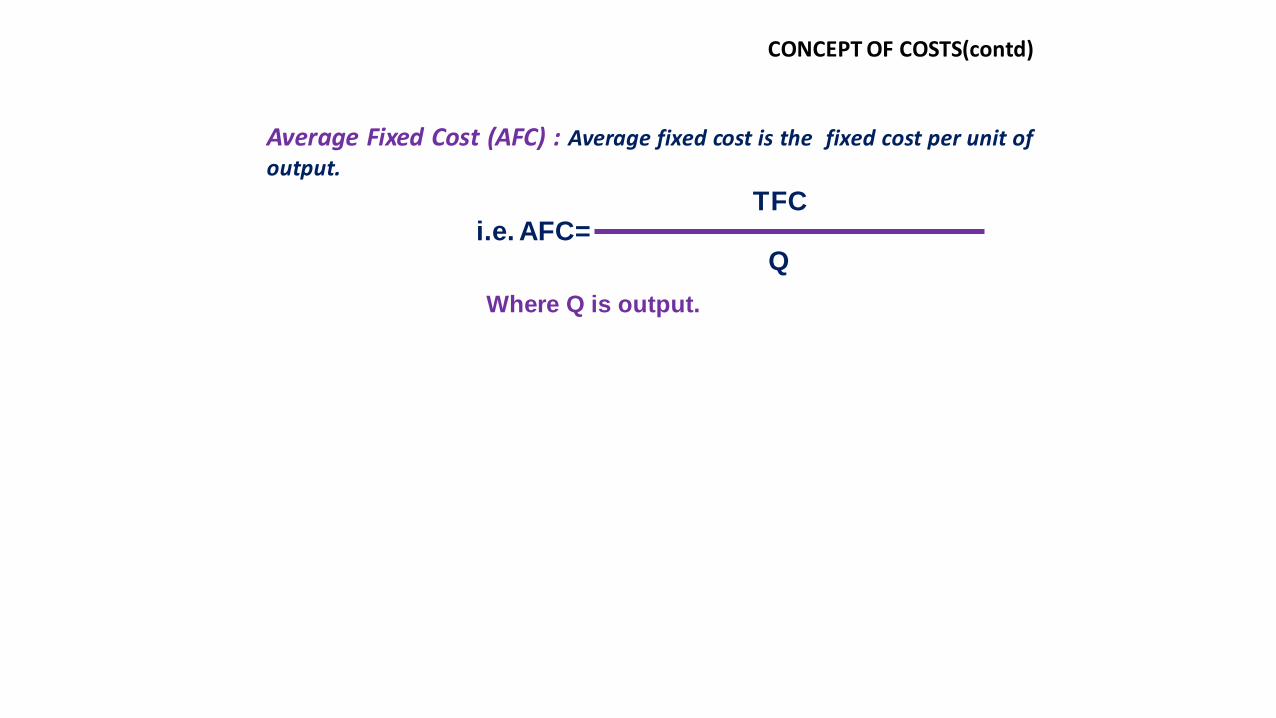
Average Fixed Cost (AFC) : Average fixed cost is the fixed cost per unit ofoutput.
i.e. AFC=TFC
Q
Where Q is output.
CONCEPT OF COSTS(contd)
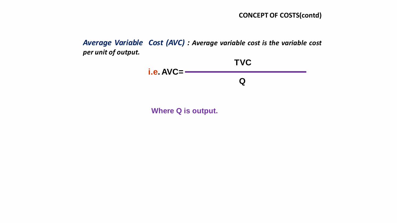
Average Variable Cost (AVC) : Average variable cost is the variable costper unit of output.
i.e. AVC=TVC
Q
Where Q is output.

CONCEPT OF COSTS(contd)
Average Cost (AC) : Average cost is the cost per unit of output.
i.e. AC=TC
Q
=
TFC+ TVC
Q
Or, AC= AFC + AVC
Where Q is output.

CONCEPT OF COSTS(contd)
Marginal cost (MC) : Marginal cost is the extra cost for producing anadditional unit of output.
i.e. MC=d(TC)
dQ
MC=d(TFC + TVC)
dQ
MC=
d(TVC)
dQ
It is important to note that marginal cost is derived solely from variable costs, and not from fixed costs.

MC
AVC
AC
AFC
Output
Cost
O
AFC, AC, AVC, MC curves CONCEPT OF COSTS(contd)

Minimum MC comes before, Minimum AC.
When AC falls, MC < AC
When AC increases, MC > AC
When AC is at its minimum, MC equals AC. i.e. MC=Minimum AC.
MC AC
Minimum ACMinimum MC
Output
Cost
Minimum
O
AVC
Minimum AVC
RELATIONSHIP BETWEEN AC AND MC
AVERAGE FIXED COST (AFC) FALLS WITH INCREASE IN OUTPUT
AFC curve is downward sloping from left to right.
REASONS
As total fixed cost is divided by an increasing output, AFC will continue to fall. AFCmay be very close to zero, but will never be equal to zero.
CONCEPT OF COSTS(contd)

AVERAGE VARIABLE COST CURVE , AVERAGE COST CURVE , AVERAGE COST CURVE areIS U-SHAPED
With the increase in output each of these curves will slope down at frist from left toright, then reach a minimum point, and rise again.
‘U’ shaped AVC , MC, AC curve can be attributed to the principle of variableproportion.
CONCEPT OF COSTS(contd)

LONG RUN AVERAGE COST FUNCTION Or
LONG RUN AVERAGE COST (LAC) CURVE
The long run cost function/LAC curve depicts the least possibleaverage cost for producing various levels of output when inputs ofproduction are variable (in the long run).
The LAC is constructed from a series of short run average costcurves associated with a series of different output levels. In short run,capital (say plant) is fixed, and labour is variable. As such, each of the shortrun average cost (SAC) curves corresponds to a particular plant. When a newplant is installed, the SAC curve shifts to a new location.
The LAC curve is the envelope of an infinite number of SAC curves,with each SAC curve tangent to the LAC curve at a single pointcorresponding to a particular output level.
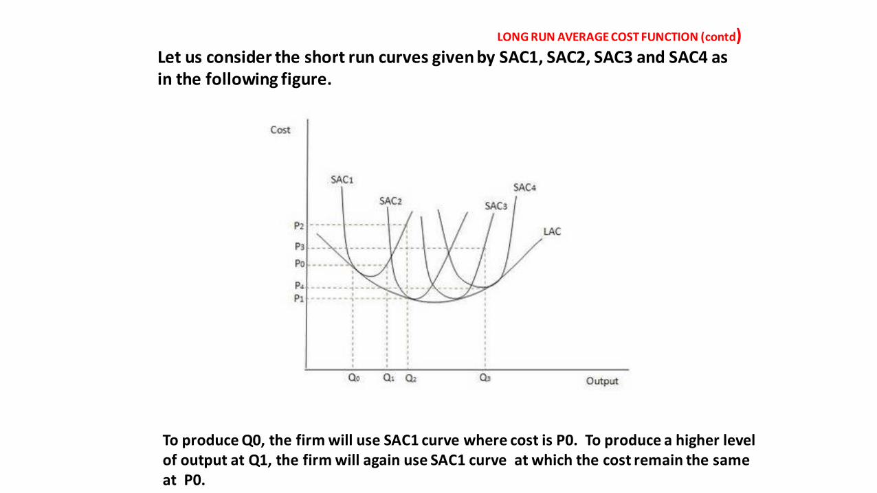
LONG RUN AVERAGE COST FUNCTION (contd)Let us consider the short run curves given by SAC1, SAC2, SAC3 and SAC4 as in the following figure.
To produce Q0, the firm will use SAC1 curve where cost is P0. To produce a higher level of output at Q1, the firm will again use SAC1 curve at which the cost remain the same at P0.

LONG RUN AVERAGE COST FUNCTION (contd)
To produce Q2, if the firm continues to use SAC1 curve, then the cost will increase toP2(P2>PO). So, it would be better for the firm to bring a second plant into the productionwith cost curve SAC2. Here, cost of producing Q2 would be P1, much less than P2.
Similarly, to Produce Q3, the firm can either use SAC3 or SAC4 curve. If it uses SAC3curve, the cost of production would be P3 which is higher than P4 at SAC4. Hence, the firmwill use SAC4 curve, as it has low cost(P4).

LONG RUN AVERAGE COST FUNCTION (contd)
The above description confirms that, in long run, a firm will use thelevel of inputs that can produce a given level of output at the lowest possibleaverage cost. The envelope relationship explains that at the planned outputlevel, SAC equals LAC; but at all other levels of output, SAC is higher than LAC.This is reflected in LAC curve which is always be less than or equal to short-run average cost.

Revenue
Samir K Mahajan, M.Sc, Ph.D.,UGC-NET

RevenueMeaning :
Revenue is the receipt of money from the sale of output by a firm in a given time period.
Concepts of Revenue
Total Revenue
Average revenue
MarginalRevenue

Total Revenue
Total Revenue (TR) is the total amount of money receipts of a firm from the
sale of output.
TR = Price X Q where Q is the output sold
TR = AR X Q = 𝑴𝑹

Average RevenueAverage Revenue (AR) is revenue per unit of output sold.
AR=Price

Marginal Revenue
Marginal Revenue (MR) is the rate of change in total revenue
with respect to change in output.
Where,
Q is output sold

Output Sold
Output Sold
Revenue
Revenue
TR
ARMR
1. When total Revenue is
maximised, MR = 0
2. AR curve is the demand
curve facing a firm in the
market
3. AR and MR curves are
downward sloping, MR
curve lies below AR
curve.
0
0
TR, AR and MR under Im-Perfect Competition

Output Sold
Output Sold
Revenue
Revenue
TR
AR=MR=Price
1. Under perfect
Competition price is
uniform and given. As
such, AR(price) and MR
become equal.
2. AR and MR curves
coincide and become
parallel to output axis.
3. AR curve i.e. the demand
curve facing a firm in the
market is perfectly elastic.
0
0
TR, AR and MR under Perfect Competition
p

PROFIT , BREAK-EVEN POINT
AND
EQUILIBRIUM OF A FIRM
Samir K Mahajan, M.Sc, Ph.D.,UGC-NET
Assistant Professor (Economics)Department of Mathematics & Humanities
Institute of Technology Nirma University

PROFIT
Profit is defined as the gap between total revenue and total cost.
Profit(∏ ) =Total Revenue – Total Cost
When profit is negative, a firm is said to be suffering from loss.
BREAK -EVEN POINT
Break-even point indicates the level of output at which Total Revenue just equals Total
Cost .
EQUILIBRIUM OF A FIRM
A firm is said to in equilibrium when it maximises its profit at given level of output.
Thus, at firm’s equilibrium, profit(TR-TC) is maximum.
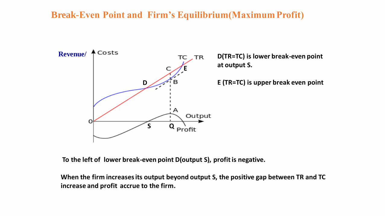
Break-Even Point and Firm’s Equilibrium(Maximum Profit)
Revenue/
D
E
Q
To the left of lower break-even point D(output S), profit is negative.
When the firm increases its output beyond output S, the positive gap between TR and TC increase and profit accrue to the firm.
S
D(TR=TC) is lower break-even point at output S.
E (TR=TC) is upper break even point

Break-Even Point and Firm’s Equilibrium(Maximum Profit) (contd.)
The firm is in equilibrium (maximum profit =CB=AQ) at Q level of output after which the gap between TR and TC goes on narrowing. TR again becomes equal to TC at upper break even point E.
Upper break-even E point is not of much relevance as it lies beyond firm's profit maximizing level.Further, it lies beyond the firm’s capacity.
The lower break even point D at output S is much significance as the firm would not plan to expand ifit can not sell its output equal to at least S.
EQUILIBRIUM OF A FIRM /PROFIT MAXIMISATION BY A FIRM : MARGINAL APPROACH
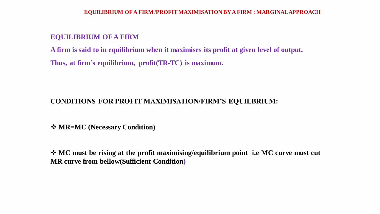
EQUILIBRIUM OF A FIRM
A firm is said to in equilibrium when it maximises its profit at given level of output.
Thus, at firm’s equilibrium, profit(TR-TC) is maximum.
CONDITIONS FOR PROFIT MAXIMISATION/FIRM’S EQUILBRIUM:
MR=MC (Necessary Condition)
MC must be rising at the profit maximising/equilibrium point i.e MC curve must cut
MR curve from bellow(Sufficient Condition)
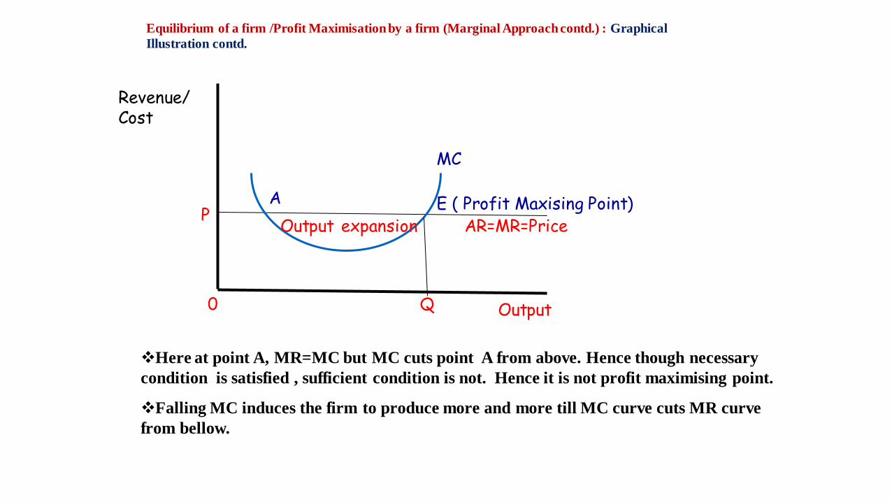
Output
Revenue/Cost
MC
Here at point A, MR=MC but MC cuts point A from above. Hence though necessary
condition is satisfied , sufficient condition is not. Hence it is not profit maximising point.
Falling MC induces the firm to produce more and more till MC curve cuts MR curve
from bellow.
0
Equilibrium of a firm /Profit Maximisation by a firm (Marginal Approach contd.) : Graphical
Illustration contd.
AP
E ( Profit Maxising Point)
Q
Output expansion AR=MR=Price

At point E , MR=MC and MC curve cuts MR curve from bellow. At E, both
necessary and sufficient conditions are satisfied. Hence E is the point of equilibrium at
which the firm maximises its profit.
Q is the equilibrium or profit maximising output. The firm will not produce beyond
point E or output Q . Because after point E, MR < MC. As a result of which the firm
will suffer loss.
Equilibrium of a firm /Profit Maximisation : Graphical Illustration (contd.)