Countercyclical Macro Prudential Policies in a Supporting Role to Monetary Policy

Papa N’Diaye

WP/09/257

© 2009 International Monetary Fund WP/09/257

IMF Working Paper

Asia and Pacific Department

Countercyclical Macro Prudential Policies in a Supporting Role to Monetary Policy

Prepared by Papa N’Diaye

Authorized for distribution by Nigel Chalk

November 2009

Abstract

This Working Paper should not be reported as representing the views of the IMF. The views expressed in this Working Paper are those of the author(s) and do not necessarily represent those of the IMF or IMF policy. Working Papers describe research in progress by the author(s) and are published to elicit comments and to further debate.

This paper explores how prudential regulations can support monetary policy in reducing output fluctuations while maintaining financial stability. It uses a new framework that blends a standard model for monetary policy analysis with a contingent claims model of financial sector vulnerabilities. The results suggest that binding countercyclical prudential regulations can help reduce output fluctuations and lessen the risk of financial instability. More specifically, countercyclical rules such as countercyclical capital adequacy rules, can allow monetary authorities to achieve the same output and inflation objectives but with smaller adjustments in interest rates. The countercyclical rules can help stem swings in asset prices, lean against a financial accelerator process, and thereby help to lower risks of macroeconomic and financial instability. In economies with fixed exchange rates, where countercyclical monetary policy is not possible, prudential regulations can provide a useful mechanism for mitigating a run-up in asset prices and for promoting output stability.

JEL Classification Numbers: E51, E58, E37, G13, G18. Keywords: Monetary policy, asset prices, macro prudentials, contingent claim analysis. Author’s E-Mail Address: pndiaye@imf.org

2

Contents Page

I. Introduction ............................................................................................................................3

II. Overview of the CCA............................................................................................................4

III. Model Overview ..................................................................................................................8 A. Aggregate Demand Equation ..................................................................................11 B. Inflation ...................................................................................................................11 C. Core Inflation—Phillips curve ................................................................................11 D. Okun’s Law Relationship........................................................................................12 E. Labor Income...........................................................................................................12 F. Exchange Rate .........................................................................................................12 G. Monetary Policy Rule .............................................................................................13 H. Yield Curve and Term Structure.............................................................................15 I. Spreads and Balance Sheets .....................................................................................15 J. Uncertainty ...............................................................................................................17 K. Debt Dynamics........................................................................................................17 L. Financial Regulations ..............................................................................................18 M. Equity .....................................................................................................................18 N. The Supply Side ......................................................................................................19

IV. Illustrative Model Simulations ..........................................................................................19

V. Conclusion ..........................................................................................................................21 References................................................................................................................................22

3

I. INTRODUCTION

The global financial crisis that followed the bursting of the credit boom and housing bubble in the United States has been characterized by a vicious self-reinforcing mechanism of deleveraging, tightened financial conditions, asset prices deflation, and output losses. In an effort to stop that vicious cycle, central banks in major economies, particularly the Fed, have lowered their policy rates to near zero and introduced a set of measures aimed at increasing liquidity and stimulating credit in domestic markets, including serving as lender of last resort for systemically important institutions, creating new central banks facilities, and buying government or corporate securities.1 While these measures have alleviated somewhat the pressure in credit markets, the persistence of the global financial crisis and the magnitude of losses that financial and non-financial institutions around the world have incurred so far illustrate the importance of macro-financial interlinkages. At the same time, the size of the contagion around the world has highlighted the risks that greater trade and financial integration can pose for macroeconomic and financial stability.

The accommodative monetary policy stances in the bulk of the world economy, combined with forceful fiscal policy responses worldwide, have helped ease the extent of the downturn and facilitate a process of economic recovery. As such, an early withdrawal of macroeconomic stimulus could put at risk the nascent global recovery. However, at the same time, these easy monetary and fiscal conditions, if protracted, have the potential to create inflation in goods and assets markets which could put at risk future macroeconomic and financial stability.

Against this backdrop, this paper analyzes the potential macroeconomic benefits of adopting countercyclical macro prudential rules to mitigate the risks of asset price inflation while safeguarding the recovery in the real economy. The analysis uses a model that integrates forward-looking indicators of balance sheet risk into a traditional multicountry country model for monetary analysis to better capture the interlinkages between financial sector and the real sector (see Gray, Karam, and N’Diaye (2009)). The model is a tool for analyzing the propagation and amplification role that credit and, more generally balance sheet conditions, can play in the transmission of shocks. The underlying idea of the modeling strategy follows the tradition of the financial accelerator process pioneered by Bernanke, Gertler, and Gilchrist (1999). Borrowing costs depend on an “external finance premium” or a spread that reflects borrowers net worth. However, distinct from other approaches,2 here we model this external finance premium drawing on the contingent claims analysis (CCA), commonly called the Merton Model.3 Such an approach helps to better capture the underlying risk as well as interactions between balance sheets, with financial distress at the corporates or

1 See October 2009 GFSR For a discussion of the measures undertaken by central banks and their impact on markets.

2 See Bernanke, Gertler and Gilchrist (1999) for a presentation of the financial accelerator and Kyotaki and Moore (1997) for a discussion on endogenous credit cycles.

3 See Merton (1998) and Gray, Merton, and Bodie (2008).

4

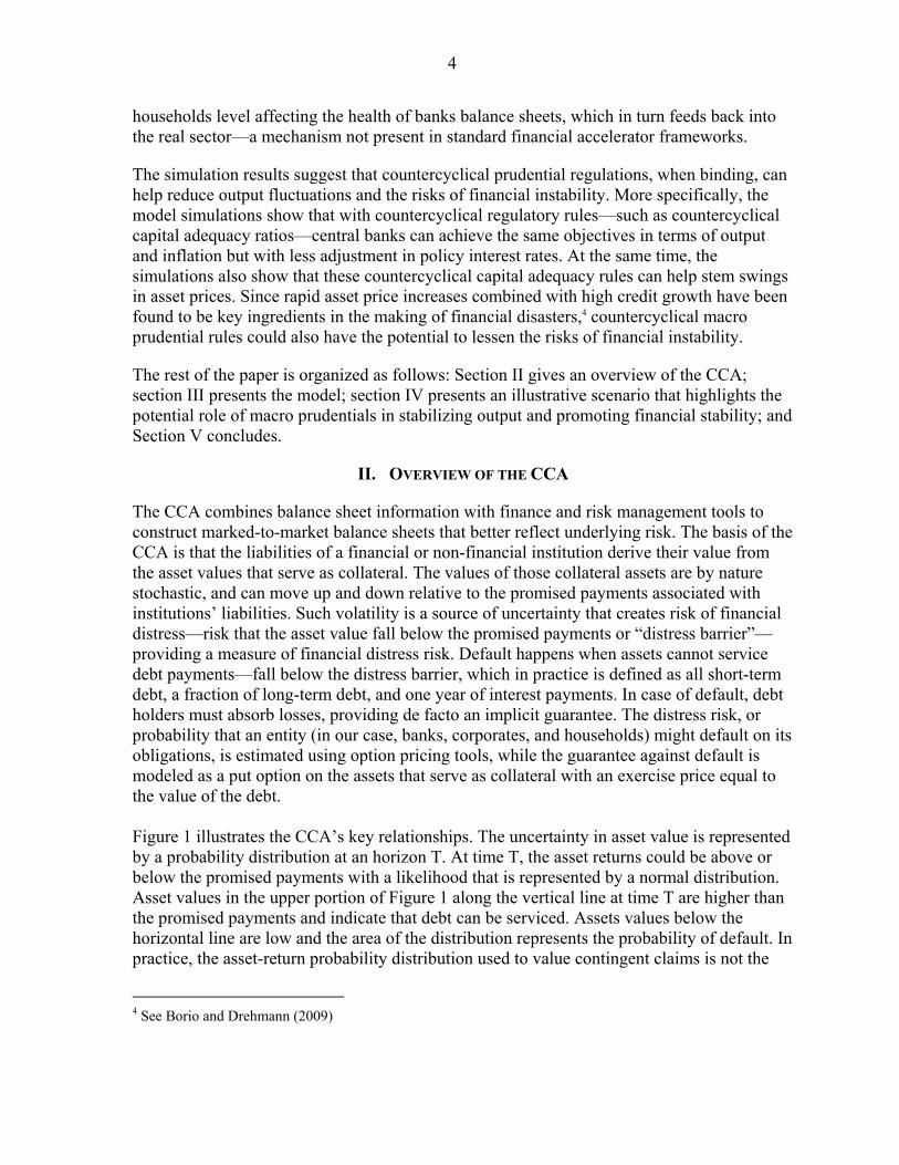
households level affecting the health of banks balance sheets, which in turn feeds back into the real sector—a mechanism not present in standard financial accelerator frameworks.

The simulation results suggest that countercyclical prudential regulations, when binding, can help reduce output fluctuations and the risks of financial instability. More specifically, the model simulations show that with countercyclical regulatory rules—such as countercyclical capital adequacy ratios—central banks can achieve the same objectives in terms of output and inflation but with less adjustment in policy interest rates. At the same time, the simulations also show that these countercyclical capital adequacy rules can help stem swings in asset prices. Since rapid asset price increases combined with high credit growth have been found to be key ingredients in the making of financial disasters,4 countercyclical macro prudential rules could also have the potential to lessen the risks of financial instability.

The rest of the paper is organized as follows: Section II gives an overview of the CCA; section III presents the model; section IV presents an illustrative scenario that highlights the potential role of macro prudentials in stabilizing output and promoting financial stability; and Section V concludes.

II. OVERVIEW OF THE CCA

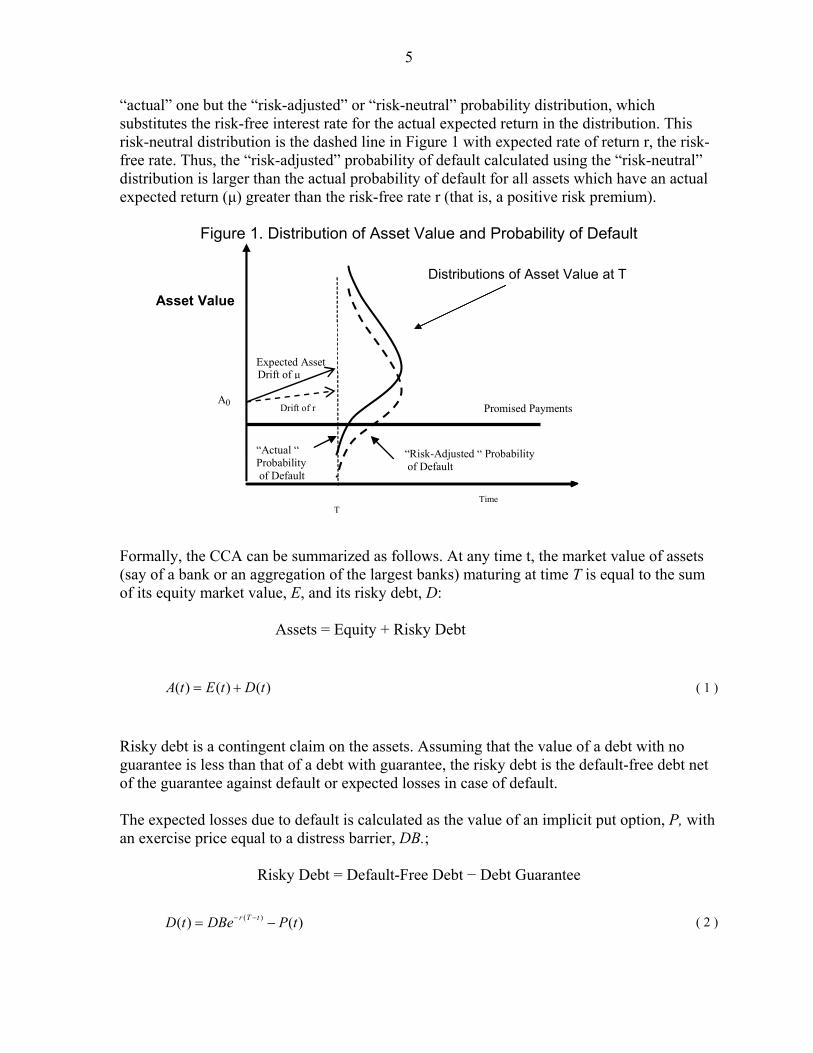
The CCA combines balance sheet information with finance and risk management tools to construct marked-to-market balance sheets that better reflect underlying risk. The basis of the CCA is that the liabilities of a financial or non-financial institution derive their value from the asset values that serve as collateral. The values of those collateral assets are by nature stochastic, and can move up and down relative to the promised payments associated with institutions’ liabilities. Such volatility is a source of uncertainty that creates risk of financial distress—risk that the asset value fall below the promised payments or “distress barrier”—providing a measure of financial distress risk. Default happens when assets cannot service debt payments—fall below the distress barrier, which in practice is defined as all short-term debt, a fraction of long-term debt, and one year of interest payments. In case of default, debt holders must absorb losses, providing de facto an implicit guarantee. The distress risk, or probability that an entity (in our case, banks, corporates, and households) might default on its obligations, is estimated using option pricing tools, while the guarantee against default is modeled as a put option on the assets that serve as collateral with an exercise price equal to the value of the debt. Figure 1 illustrates the CCA’s key relationships. The uncertainty in asset value is represented by a probability distribution at an horizon T. At time T, the asset returns could be above or below the promised payments with a likelihood that is represented by a normal distribution. Asset values in the upper portion of Figure 1 along the vertical line at time T are higher than the promised payments and indicate that debt can be serviced. Assets values below the horizontal line are low and the area of the distribution represents the probability of default. In practice, the asset-return probability distribution used to value contingent claims is not the

4 See Borio and Drehmann (2009)

5

“actual” one but the “risk-adjusted” or “risk-neutral” probability distribution, which substitutes the risk-free interest rate for the actual expected return in the distribution. This risk-neutral distribution is the dashed line in Figure 1 with expected rate of return r, the risk-free rate. Thus, the “risk-adjusted” probability of default calculated using the “risk-neutral” distribution is larger than the actual probability of default for all assets which have an actual expected return (μ) greater than the risk-free rate r (that is, a positive risk premium).

Figure 1. Distribution of Asset Value and Probability of Default

Asset Value

Expected Asset

Distributions of Asset Value at T

Drift of μ

Promised Payments A0

T Time

“Actual “ Probability of Default

Drift of r

“Risk-Adjusted “ Probability of Default

Formally, the CCA can be summarized as follows. At any time t, the market value of assets (say of a bank or an aggregation of the largest banks) maturing at time T is equal to the sum of its equity market value, E, and its risky debt, D:

Assets = Equity + Risky Debt

( ) ( ) ( )A t E t D t ( 1 )

Risky debt is a contingent claim on the assets. Assuming that the value of a debt with no guarantee is less than that of a debt with guarantee, the risky debt is the default-free debt net of the guarantee against default or expected losses in case of default. The expected losses due to default is calculated as the value of an implicit put option, P, with an exercise price equal to a distress barrier, DB.;

Risky Debt = Default-Free Debt − Debt Guarantee

( )( ) ( )r T tD t DBe P t ( 2 )

6

2 1

1 2

rTt

A

P DBe N d AN d

where d d T

( 3 )

r denotes the risk free rate and A is the asset return volatility, N is the cumulative normal

distribution. 2d is the distance-to-distress and is generally specified as:

22 0

1ln / /

2t A Ad A DB r T T ( 4 )

Using equations (1)–(4), the probability that asset values fall below DB is:

2tPD N d ( 5 )

And the spread is given by

1

ln 1 tt rT

PSpread

T DBe

( 6 )

The CCA is well suited for analyzing most balance sheet effects and their interaction with macroeconomic variables. The spread or external finance premium increases with the volatility of assets as well as maturity and currency mismatches in sectoral balance sheets, which helps to analyze the balance sheet effects of uncertainty, funding difficulties, interest rate and exchange rate changes, shocks to asset returns, shocks to GDP growth and employment—as well as the feedback loop that exist between them.

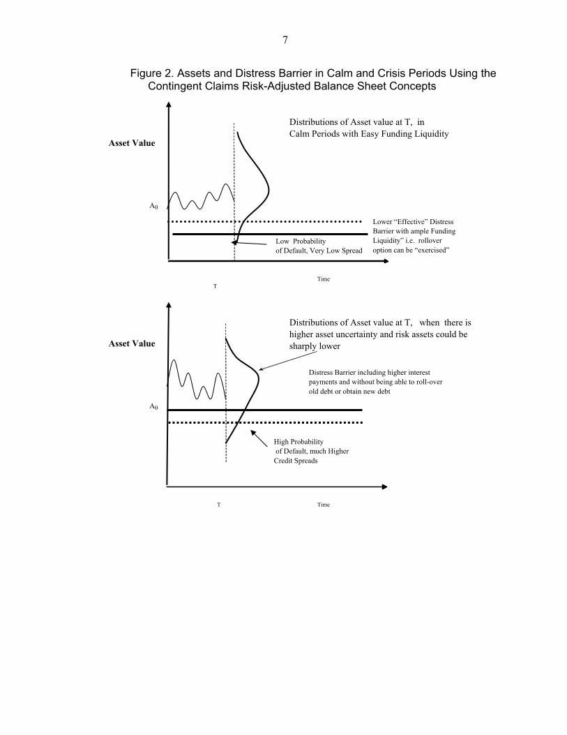
Figure 2 illustrates the key relationships between changes in balance sheet assets, asset volatility, and changes in the distress/default barrier due to shifts in short-and long-term debt or funding liquidity. The uncertainty in asset value is represented by a probability distribution at time horizon T. In periods of high market liquidity, short-term debt can be easily rolled over and thus the effective default barrier is lower (Figure 2, first panel). However, in periods of stress, asset values are lower and, if assets are illiquid, there is a risk that they might need to be sold at a sharp discount (Figure 2, second panel). That risk of a sharp decline in asset values implies a fat tail in the probability distribution of the assets. The combination of a probability distribution of assets with a fatter tail and the higher default barrier imply a much higher probability of default and larger credit spreads than when volatility is low. By the same token, the more illiquid the assets, the higher the risk that asset values will decline substantially (a fatter tail) and the higher credit spreads.

7

Asset Value

Distributions of Asset value at T, in Calm Periods with Easy Funding Liquidity

Lower “Effective” Distress Barrier with ample Funding Liquidity” i.e. rollover option can be “exercised”

A0

T

Time

Low Probability of Default, Very Low Spread

Asset Value

Distributions of Asset value at T, when there is higher asset uncertainty and risk assets could be sharply lower

Distress Barrier including higher interest payments and without being able to roll-over old debt or obtain new debt

A0

T

Time

High Probability of Default, much Higher Credit Spreads

Figure 2. Assets and Distress Barrier in Calm and Crisis Periods Using the Contingent Claims Risk-Adjusted Balance Sheet Concepts

8

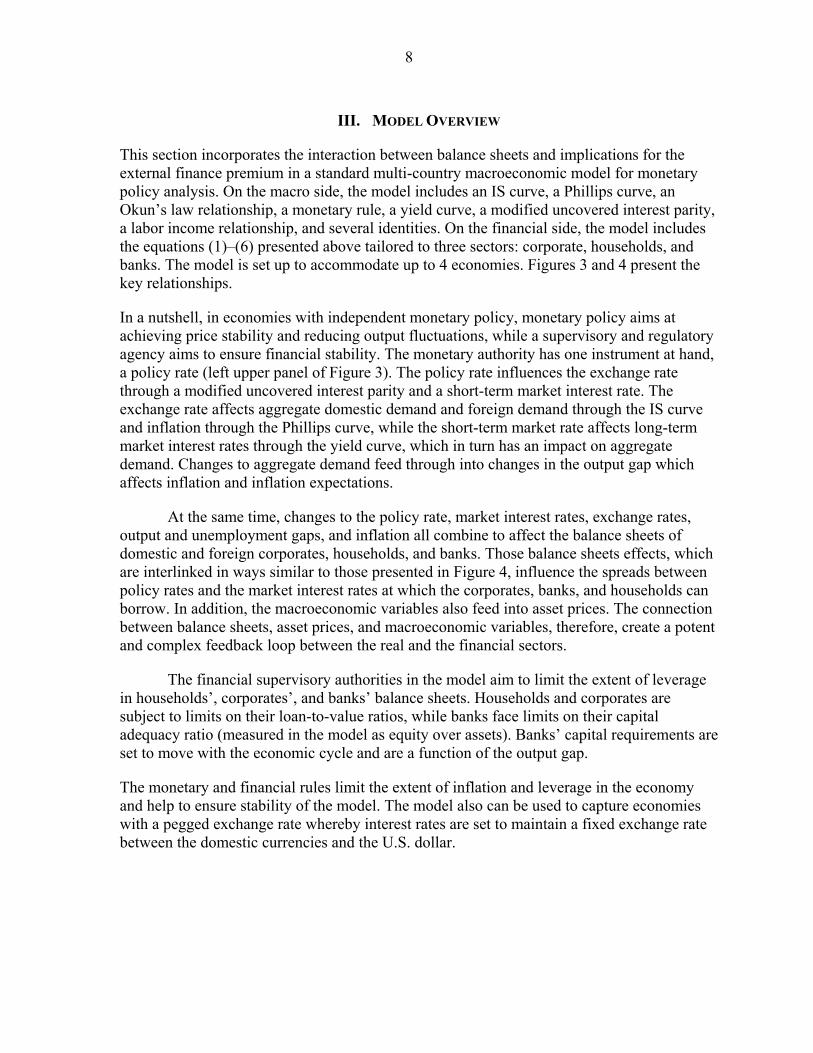
III. MODEL OVERVIEW

This section incorporates the interaction between balance sheets and implications for the external finance premium in a standard multi-country macroeconomic model for monetary policy analysis. On the macro side, the model includes an IS curve, a Phillips curve, an Okun’s law relationship, a monetary rule, a yield curve, a modified uncovered interest parity, a labor income relationship, and several identities. On the financial side, the model includes the equations (1)–(6) presented above tailored to three sectors: corporate, households, and banks. The model is set up to accommodate up to 4 economies. Figures 3 and 4 present the key relationships.

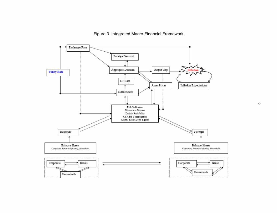
In a nutshell, in economies with independent monetary policy, monetary policy aims at achieving price stability and reducing output fluctuations, while a supervisory and regulatory agency aims to ensure financial stability. The monetary authority has one instrument at hand, a policy rate (left upper panel of Figure 3). The policy rate influences the exchange rate through a modified uncovered interest parity and a short-term market interest rate. The exchange rate affects aggregate domestic demand and foreign demand through the IS curve and inflation through the Phillips curve, while the short-term market rate affects long-term market interest rates through the yield curve, which in turn has an impact on aggregate demand. Changes to aggregate demand feed through into changes in the output gap which affects inflation and inflation expectations.

At the same time, changes to the policy rate, market interest rates, exchange rates, output and unemployment gaps, and inflation all combine to affect the balance sheets of domestic and foreign corporates, households, and banks. Those balance sheets effects, which are interlinked in ways similar to those presented in Figure 4, influence the spreads between policy rates and the market interest rates at which the corporates, banks, and households can borrow. In addition, the macroeconomic variables also feed into asset prices. The connection between balance sheets, asset prices, and macroeconomic variables, therefore, create a potent and complex feedback loop between the real and the financial sectors.

The financial supervisory authorities in the model aim to limit the extent of leverage in households’, corporates’, and banks’ balance sheets. Households and corporates are subject to limits on their loan-to-value ratios, while banks face limits on their capital adequacy ratio (measured in the model as equity over assets). Banks’ capital requirements are set to move with the economic cycle and are a function of the output gap.

The monetary and financial rules limit the extent of inflation and leverage in the economy and help to ensure stability of the model. The model also can be used to capture economies with a pegged exchange rate whereby interest rates are set to maintain a fixed exchange rate between the domestic currencies and the U.S. dollar.

9

Figure 3. Integrated Macro-Financial Framework

10

Figure 4. Integrated Macro-Financial Framework: Balance Sheet Interlinkages

11

The details of the model are as follows.5

A. Aggregate Demand Equation

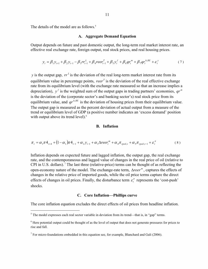
Output depends on future and past domestic output, the long-term real market interest rate, an effective real exchange rate, foreign output, real stock prices, and real housing prices.

yt

REht

mt

ft

Tt

Ltttt qrqryreerrryyy

,76514131211 ( 7 )

y is the output gap, Lrr is the deviation of the real long-term market interest rate from its

equilibrium value in percentage points, Treer is the deviation of the real effective exchange rate from its equilibrium level (with the exchange rate measured so that an increase implies a depreciation), fy is the weighted sum of the output gaps in trading partners’ economies, mqr is the deviation of the (corporate sector’s and banking sector’s) real stock price from its equilibrium value, and REhqr , is the deviation of housing prices from their equilibrium value. The output gap is measured as the percent deviation of actual output from a measure of the trend or equilibrium level of GDP (a positive number indicates an ‘excess demand’ position with output above its trend level).6

B. Inflation

ttrpoiltrpoilm

ttttt reery 1,5,43121141 414 ( 8 )

Inflation depends on expected future and lagged inflation, the output gap, the real exchange rate, and the contemporaneous and lagged value of changes in the real price of oil (relative to CPI in U.S. dollars). 7 The last three (relative-price) terms can be thought of as reflecting the open-economy nature of the model. The exchange-rate term, mreer , captures the effects of changes in the relative price of imported goods, while the oil price terms capture the direct effects of changes in oil prices. Finally, the disturbance term t

represents the ‘cost-push’

shocks.

C. Core Inflation—Phillips curve

The core inflation equation excludes the direct effects of oil prices from headline inflation.

5 The model expresses each real sector variable in deviation from its trend—that is, in “gap” terms.

6 Here potential output could be thought of as the level of output that does not generate pressures for prices to rise and fall.

7 For micro-foundations embedded in this equation see, for example, Blanchard and Gali (2006).

12

The equation for core inflation is:

ttctcm

tctctcctcctc reery 1,14,3,12,1,1,4,1,, 44414 ( 9 )

Core inflation, ,c t , depends on expected future and lagged inflation, the output gap

(demand-pull forces), the real exchange rate (import-weighted real exchange rate, mreer in

difference terms), and an additional term 1 , 14 4t c t that allows for the possibility of

relative price and real wage resistance; or more precisely that workers and other price setters may try to align their prices to past movements in headline CPI.8 The exchange-rate pass-through coefficient, 3,c , is assumed to be the same as in the headline inflation equation.

Note that under a long-run relative Purchasing Power Parity (PPP) condition, ongoing inflation differentials between a country and its trading partner can persist with the differential being reflected in the trend movement in the nominal exchange rate. However, in the short-term, because of the backward-looking component of expected exchange rate (equation (13)), shocks that affect the nominal exchange rate will also affect the real exchange rate during a transition period.

D. Okun’s Law Relationship

The Okun equation links the movements in unemployment to those in the output gap. Some degree of persistence in the dynamics of the unemployment gap is captured by the presence of the lagged values of unemployment gap.

ugaptttt ygapugapugap 1211 (10)

E. Labor Income

Aggregate households’ labor income increases with output and declines with the unemployment rate.

LIttutyt UYLI (11)

F. Exchange Rate

The exchange rate equation (12) is the uncovered interest parity (UIP), an arbitrage condition equalizing the effective rates of return on investments (defined as the rate of return net of changes in the exchange rate) in different currencies, accounting for country-specific risk premiums. One feature of this equation is that a foreign investor expecting a

8 See Hunt, Isard, and Laxton (2003).

13

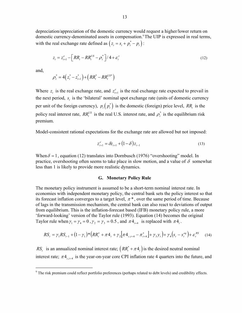
depreciation/appreciation of the domestic currency would request a higher/lower return on domestic currency-denominated assets in compensation.9 The UIP is expressed in real terms,

with the real exchange rate defined as *t t t tz s p p :

*1 / 4e US z

t t t t t tz z RR RR (12)

and,

* * * * *14 US

t t t t tz z RR RR

Where tz is the real exchange rate, and 1

etz is the real exchange rate expected to prevail in

the next period, ts is the ‘bilateral’ nominal spot exchange rate (units of domestic currency

per unit of the foreign currency), *t tp p is the domestic (foreign) price level, tRR is the

policy real interest rate, UStRR is the real U.S. interest rate, and *

t is the equilibrium risk

premium.

Model-consistent rational expectations for the exchange rate are allowed but not imposed: 111 1 tt

et zzz (13)

When 1 , equation (12) translates into Dornbusch (1976) “overshooting” model. In practice, overshooting often seems to take place in slow motion, and a value of somewhat less than 1 is likely to provide more realistic dynamics.

G. Monetary Policy Rule

The monetary policy instrument is assumed to be a short-term nominal interest rate. In economies with independent monetary policy, the central bank sets the policy interest so that its forecast inflation converges to a target level, * , over the same period of time. Because of lags in the transmission mechanism, the central bank can also react to deviations of output from equilibrium. This is the inflation-forecast based (IFB) monetary policy rule, a more ‘forward-looking’ version of the Taylor rule (1993). Equation (14) becomes the original Taylor rule when 1 4 0 , 5.032 , and 44t is replaced with 4t .

RSt

eqtttttctttt ssyRRRSRS

4344,2111 44*1 (14)

tRS is an annualized nominal interest rate; * 4t tRR is the desired neutral nominal

interest rate; , 44c t is the year-on-year core CPI inflation rate 4 quarters into the future, and

9 The risk premium could reflect portfolio preferences (perhaps related to debt levels) and credibility effects.

14

*4t is the year-on-year target inflation 4 quarters into the future. The structure and

parameters of this equation have a variety of implications.10 The larger the parameters 2 and

3 , the more aggressive the policy reaction to any deviation of inflation to its target, output

gap, or deviation of the exchange rate from its desired level. For the dynamics of inflation to be stable, the Taylor principle has to apply. In practice, the extent to which central banks react to fluctuations in output or inflation hinges on other characteristics of the economy, in particular the degree to which agents are forward looking and how well inflation expectations are anchored. In economies with forward-looking agents, moderate but persistent reactions of interest rates to expected inflation could still be sufficient to keep inflation close to target. The policy response can also be smoothed with gradual adjustment of interest rates in response to deviations of inflation and output from equilibrium.

In economies with a fixed exchange rate, 11 and 4 . This maintains a fixed bilateral exchange rate, with domestic interest rates set such that the exchange bilateral rate is at its desired level (here assumed to be its one period lagged value).

In general, other arguments than inflation, output, or the exchange rate could be considered in the monetary reaction function (14)—this is the case of asset prices (property or equity prices). While adding asset prices to the monetary reaction function is not very challenging from a theoretical point of view, it is difficult to implement such a policy in practice. Policy-makers would need to know whether asset prices are misaligned and how to react to such a situation (whether they should lean against a forming bubble or ease in anticipation of the bursting of such a bubble). As such, explicitly targeting asset prices has been considered unappealing in the literature.11 Many consider that the instruments of monetary policy are too blunt to be used effectively for controlling asset-price bubbles. Moreover, to the extent that asset prices affect output, there may be no reason for monetary policy to react above and beyond what is required to stabilize output and inflation. The logic would suggest that when faced with a forming asset prices bubble the best course of action is to react strongly once the bubble has burst in order to limit the negative output effects. This was the predominant view amongst policymakers before the global financial crisis broke out. However, now with the benefits of hindsight, policy makers and observers are increasingly viewing that the rigid pursuit of an inflation target could encourage the build up of imbalances in markets other than the goods market, particularly when expectations take hold that monetary conditions will remain loose for a prolonged period of time.12

10 For a brief introduction to the vast literature evaluating alternative monetary policy rules see Hunt and Orr (1999) and Taylor (1999).

11 See Bernanke (2002), Greenspan (2004), and Selody and Wilkins (2004).

12 On the subject of the role of monetary policy under credit constraints, Cúrdia and Woodford (2008) consider a “spread-adjusted Taylor rule”, in which the intercept of the Taylor rule is adjusted with changes in credit spreads. See also Gray and Malone (2008).

15

H. Yield Curve and Term Structure

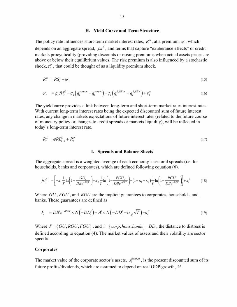
The policy rate influences short-term market interest rates, mR , at a premium, , which

depends on an aggregate spread, Efsi , and terms that capture “exuberance effects” or credit markets procyclicality (providing discounts or raising premiums when actual assets prices are above or below their equilibrium values. The risk premium is also influenced by a stochastic shock, t

, that could be thought of as a liquidity premium shock.

ttmt RSR (15)

, , , , , ,1 2 3

E corp m corp h RE m h REt t t t t t tfsi q q q q (16)

The yield curve provides a link between long-term and short-term market rates interest rates. With current long-term interest rates being the expected discounted sum of future interest rates, any change in markets expectations of future interest rates (related to the future course of monetary policy or changes to credit spreads or markets liquidity), will be reflected in today’s long-term interest rate.

mt

Lt

Lt RRLR 1 (17)

I. Spreads and Balance Sheets

The aggregate spread is a weighted average of each economy’s sectoral spreads (i.e. for households, banks and corporates), which are defined following equation (6).

1 2 1 2

1 1 1ln 1 ln 1 1 ln 1

t t t t

E fsit t ttRS T RS T RS T

GU FGU RGUfsi

T DBe T DBe T DBe

(18)

Where GU , FGU , and RGU are the implicit guarantees to corporates, households, and banks. These guarantees are defined as

i

i RS T i i i Pt t t t tA

P DB e N DD A N DD T (19)

Where , ,P GU RGU FGU , and , ,i corp hous banks . DD , the distance to distress is

defined according to equation (4). The market values of assets and their volatility are sector specific. Corporates

The market value of the corporate sector’s assets, ,corp mtA , is the present discounted sum of its

future profits/dividends, which are assumed to depend on real GDP growth, G .

16

,

1 2 1,

11 / 400

corp

corp mt tcorp m A

t tmt

DV AA

R

(20)

With 1 1

DVt t t tDV DV G . This market value of assets can differ from its equilibrium or

trend value, ,*corptA , defined as follows.

,*

1

* ,*2 1,*

11 / 400

corpt

corptcorp A

t tmt

DV AA

R

(21)

1 1t t t

DVtDV DV G

, where *G is real potential GDP growth.

Households

Households own shares in the corporate sectors, corpQ , real estate assets, ,h REtA , and have

deposits in banks. In the CCA framework, this means that households have a claim on the risk free debt of the banks in domestic and foreign economies. Households also have labor income, LI , of which the present discounted value of the future stream is households’ human asset, LIA . Households’ total asset, HousA , is given by the following equation.13

,

t

Hous banks h RE corp LIt t t t tA DB FGU A Q A (22)

The market value of households’ real estate and their labor income assets are the present discounted sum of future rents and labor income, respectively, which in turn depend on real GDP growth and employment.

1 1

11 / 400

i

it i ti A

t tmt

X AA

R

(23)

With, , R ;i h E LI , ,X rent LI , 1

rentt t i t trent rent G , and LI defined by (11).

The equilibrium values of housing and labor income assets are given by

*

*1 1*

11 / 400

i

it i ti A

t tmt

X AA

R

(24)

With 1 2t t

rentt trent rent G

and defined by (11) and LIttuy UYLI

tt ** , where

U is the NAIRU.

13 Equation (22) would take a slightly different form if households’ hold international assets.

17

Banks

Banks assets are made of loans to households and corporates at home and abroad, which provide them with junior claims on their assets.

t

banks Corp Houst t t t tA DB GU DB RGU FGU (25)

J. Uncertainty

The volatility of assets is derived from the volatility of equity using the Black-Scholes formula.

i

i

it

i QA t

t i it A

Q

A N DD T

(26)

With ; ;i corp banks hRE . For households’ assets, the volatility is derived from

equation (22) and depends on the volatility of the corporate sector’s equity, real estate assets and labor income.

, ,

,

2 2 2

2 ,

, ,

2

2 2

corp h RE LI corp h RE

hous

corp LI h RE LI

Q A A Q At t t corp RE t tA

tQ A A A

corp LI t t RE LI t t

(27)

K. Debt Dynamics

Each sector’s debt is constituted of short-term, STD , and long-term debt, LTD , that can be denominated in domestic or foreign currencies. The following equations define the debt dynamics.

1

,, ,1

1

1400

t

t

ST FXUSST FX ST FXt

t tt

DRMD s ND

s

(28)

1

,, ,1

1

1400

t

t

LT FXUSLT FX LT FXt

t tt

DRLD s ND

s

(29)

1

, , ,11400t t

ST Dom ST Dom ST Domtt

RMD D ND

(30)

18

1

, , ,11400t t

LT Dom LT Dom LT Domtt

RLD D ND

(31)

L. Financial Regulations

The contracting of new debt (ND ) is governed by the financial regulator that impose limits on banks’ capital and households’ and corporates loans-to-value ratios.

t

ygapcarbanks

banks

banks

banks

carForSTBanks

tDomSTBanks

tBankst

yA

Q

A

QNDND

A,,,,1

(32)

Where , , , ,_ _

Bank ST FOR BANK ST DOMt NDBANK DOM FOR tND ND .

, , , , arg1 ii ST Dom i ST For T ettt t LTVi i

t t

DND ND LTV

A A

(33)

With , , , ,

_ _i ST FOR i ST DOMt NDi DOM FOR tND ND , and ,i Hous corp .

Banks are required to maintain a given amount of capital by holding some form of hybrid debt. For banks, the required amount of capital increases with the cycle (output gap). Banks keep the hybrid debt to maintain their leverage ratio at a desired level during booms and convert the hybrid debt into equity during downturns. Holding of more hybrid debt during boom times increases the leverage that back assets, lowers equity, raises the external finance premium, and tightens financial conditions. Tighter financial conditions lower banks’ asset values (through lower output) and raises the cost of servicing their debt. At the same time, households’ and corporates’ borrowing is constrained by the need to maintain a given loan-to-value ratio which limits their ability to leverage during the cycle. These loan-to-value rules could also depend on the cycle (although this possibility is not explored in this paper).

M. Equity

Equity values (both market and fundamental values) are defined here as the difference between assets and risky debt following equation (1).

, ( )t

t t t

RS Ti m i itQ A DB e GU (34)

, ( )t

t t t

RS Ti m i itQ A DB e GU (35)

With ; ;i corp banks hRE . The equity values are then transformed into two indices, one

that represents the corporate and banking sector (weighted average of the two) and one that represents the housing sector.

19

N. The Supply Side

The model has all but a rudimentary supply side. Only deviations from equilibrium levels are modeled. The supply-side variables are assumed to follow simple stochastic processes. Most key supply-side variables depend only on their own lagged values and shocks. Nonetheless, some supply side effects of oil prices on trend output have been considered. The trends are measured using the LRX filter, to allow judgment particularly toward the end of the historical data range.14

IV. ILLUSTRATIVE MODEL SIMULATIONS

This section looks at the role of countercyclical prudential regulations in reducing output fluctuations.15 It does so by considering a scenario where domestic demand exogenously expands for a couple of quarters and then by comparing the paths of output and asset prices with and without countercyclical prudential regulations.

The simulations results show that countercyclical prudential regulations can help lower output fluctuations and alleviate the burden of adjustment that lies on monetary authorities. In the model, such regulations, when binding, also stem increases in asset prices during boom times and, as a corollary, limits the asset price drop during downturns (and thus lowers the risks of financial instability).

Propagation Mechanism

The mechanisms at play are as follows. Stronger domestic demand raises corporates profits and the value of corporate assets (which are held by both banks and households). As the corporates’ assets rise their available collateral increases which, in turn, lowers their credit risk. This reduces the borrowing costs of the firm. At the same time, the initial demand shock raises household income and lowers unemployment. This also adds to the increase in the value of household assets and lowers household credit risk. As a result, the financing costs of the household also decline.

14 The technical details of the LRX filter are explained in Appendix III of Berg, Karam, and Laxton (2006). It provides a simple generalized version of the original Hodrick-Prescott filter that allows the analyst to impose priors for the trend values in situations where they believe they have useful information that would not be captured otherwise.

15 Since we are only interested in the broad properties of the model in deviation from baseline, we do not discuss here the model’s calibration. See Gray, Karam, and N’Diaye (2009) for a presentation of the model’s calibration.

20

Overall financial conditions ease. However, at the same time, the demand boom increases the risk of inflation causing monetary policy to be tightened.

Countercyclical Regulations

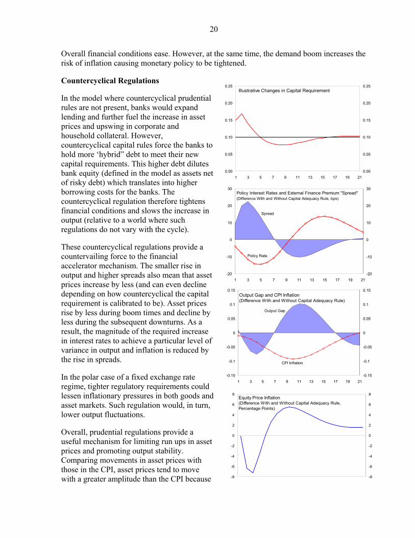
In the model where countercyclical prudential rules are not present, banks would expand lending and further fuel the increase in asset prices and upswing in corporate and household collateral. However, countercyclical capital rules force the banks to hold more ‘hybrid” debt to meet their new capital requirements. This higher debt dilutes bank equity (defined in the model as assets net of risky debt) which translates into higher borrowing costs for the banks. The countercyclical regulation therefore tightens financial conditions and slows the increase in output (relative to a world where such regulations do not vary with the cycle).

These countercyclical regulations provide a countervailing force to the financial accelerator mechanism. The smaller rise in output and higher spreads also mean that asset prices increase by less (and can even decline depending on how countercyclical the capital requirement is calibrated to be). Asset prices rise by less during boom times and decline by less during the subsequent downturns. As a result, the magnitude of the required increase in interest rates to achieve a particular level of variance in output and inflation is reduced by the rise in spreads.

In the polar case of a fixed exchange rate regime, tighter regulatory requirements could lessen inflationary pressures in both goods and asset markets. Such regulation would, in turn, lower output fluctuations.

Overall, prudential regulations provide a useful mechanism for limiting run ups in asset prices and promoting output stability. Comparing movements in asset prices with those in the CPI, asset prices tend to move with a greater amplitude than the CPI because

Illustrative Changes in Capital Requirement

0.00

0.05

0.10

0.15

0.20

0.25

1 3 5 7 9 11 13 15 17 19 21

0.00

0.05

0.10

0.15

0.20

0.25

-20

-10

0

10

20

30

1 3 5 7 9 11 13 15 17 19 21

-20

-10

0

10

20

30

Policy Rate

Spread

Policy Interest Rates and External Finance Premium "Spread"(Difference With and Without Capital Adequacy Rule, bps)

Output Gap and CPI Inflation(Difference With and Without Capital Adequacy Rule)

-0.15

-0.1

-0.05

0

0.05

0.1

0.15

1 3 5 7 9 11 13 15 17 19 21

-0.15

-0.1

-0.05

0

0.05

0.1

0.15

Output Gap

CPI Inflation

-8

-6

-4

-2

0

2

4

6

8

-8

-6

-4

-2

0

2

4

6

8Equity Price Inflation(Difference With and Without Capital Adequacy Rule, Percentage Points)

21

of their more forward looking nature and lower levels of stickiness in the model.

V. CONCLUSION

This paper showed that countercyclical macro prudential rules, such as countercyclical capital adequacy rules, could support monetary policy in reducing output fluctuations while maintaining financial stability. Specifically, the simulations show that with binding countercyclical regulatory rules monetary authorities can achieve the same objectives (in terms of deviation of output and inflation from targets) but with smaller adjustments in interest rates. The simulations also show that countercyclical capital adequacy rules can help mitigate swings in asset prices and, potentially, lower the risks of financial instability. Nevertheless, implementing and appropriately calibrating countercyclical macro prudential rules to individual country circumstances may be complex, particularly in cases where banks already exceed the existing capital adequacy requirements.

22

References

Bernanke, B., 2002, “Asset-Price ‘Bubbles’ and Monetary Policy,” remarks before the of the National Association for Business Economics , New York Chapter, October.

Bernanke, B., M. Gertler, and S. Gilchrist, 1999, “The Financial Accelerator in a Quantitative Business Cycle Framework,” in Handbook of Macroeconomics, ed. by J. Taylor and M. Woodford (Amsterdam: Elsevier).

Blanchard, O., and J. Gali, 2006, “A New Keynesian Model with Unemployment,” draft, National Bureau of Economic Research.

Berg, A., P. Karam, and D. Laxton, 2006, “Practical Model-Based Monetary Policy Analysis—A How-To Guide,” IMF Working Paper 06/81 (Washington: International Monetary Fund).

Borio, C and M Drehmann (2009) “Assessing the risk of banking crises – revisited”, BIS Quarterly Review, March, pp. 29-46.

Gray, Dale, and Samuel Malone, 2008, “Macrofinancial Risk Analysis,” (West Suxxex: Wiley Finance).

Gray, D., R. C. Merton, and Z. Bodie, 2008, “A New Framework for Measuring and Managing Macrofinancial Risk and Financial Stability,” Harvard Business School WP 09-015.

Greenspan, Alan, 2004, “Risk and Uncertainty in Monetary Policy,” American Economic Association Papers and Proceedings, Vol. 94, No. 2, pp. 33–40.

Hunt, B., P. Isard, and D. Laxton, 2003, “Inflation Targeting and the Role of the Exchange Rate,” (unpublished; Washington: International Monetary Fund).

Hunt, B., and A. Orr, 1999, “Monetary Policy Under Uncertainty,” Reserve Bank of New Zealand Conference (Wellington: Reserve Bank of New Zealand).

Karam, P, D. Gray, and P. N’Diaye, 2009, “Integrating Macro-Financial Sector Analysis,” forthcoming, IMF Working Paper (Washington: International Monetary Fund).

Kiyotaki, N., and J. Moore, 1997, “Credit Cycles,” Journal of Political Economy, Vol. 105, pp. 211–48.

Merton, R.C. , 1998, “Applications of Option-Pricing Theory: Twenty-Five Years Later,” Les Prix Nobel 1997, Stockholm: Nobel Foundation; reprinted in American Economic Review, Vol. 88 (June), pp. 323–49.

Selody, J, and C. Wilkins, 2004, “Asset Prices and Monetary Policy: A Canadian Perspective On The Issues,” Bank of Canada Review, Vol. 2004 (Autumn), pp. 3–14..

Taylor, J, ed., 1999, Monetary Policy Rules (Chicago: University of Chicago Press).