craig farnden - british columbia farnden, march 2009. survey simulator user guide v. 4.0 ii table of...

1

Craig Farnden

March 2009

Survey Simulator User Guide v. 4.0

i

Conditions

This document and the associated Excel workbook are provided free of charge on an as-is basis.

Usage implies acceptance of the following conditions:

1. No warranty can be assumed.

2. Users are solely responsible for the outcomes.

3. All modifications to the macro code and fit statistics for local calibrations must be made

publicly available on a free-of-charge basis.

4. All reports and publications using outcomes from the workbook must include an explicit

and forthright acknowledgement of usage.

Acknowledgements

The Silviculture Survey Simulator was developed as part of a PhD project at the University of

British Columbia. Funding for the project was provided by the BC Government‟s Forest

Investment Account through a delivery agreement with Canadian Forest Products Ltd., Fort St.

John. Gratefully acknowledged are the patience, guidance and advice of my supervisory

committee (Bruce Larson, Peter Marshall and John Nelson), staff at the BC Ministry of Forests

and Range - Forest Practices Branch, and staff of Canadian Forest Products Ltd, BC Timber

Sales and the BC Ministry of Forests in the Peace River region of British Columbia

Craig Farnden, March 2009


ii

Table of Contents

Introduction ..........................................................................................................1

System Requirements

Creating Stands ............................................................................................................. 2

Horizontal Complexity Layers .............................................................................................3

Vertical Structure and Species Composition .......................................................................8

Generating the TreeList .....................................................................................................11

Evaluating Generated Stands .................................................................................... 11

Stem Map ..........................................................................................................................11

Ripley‟s Spatial Indices .....................................................................................................12

Spacing Factor ...................................................................................................................14

Surveys ........................................................................................................................ 16

TreeLists for Growth modeling .................................................................................. 18

References ................................................................................................................... 19

Appendix 1: Tree Attributes ....................................................................................... 20

Appendix 2: Sub-Models ............................................................................................ 22

Appendix 3: Batch runs .............................................................................................. 28

Appendix 4: Coding New Surveys ............................................................................. 29

Appendix 5: Coding New Modeling TreeLists .......................................................... 33


1

Introduction

The Silviculture Survey Simulator is an MS Excel workbook that is used to generate realistic

stem maps of juvenile stands, and to simulate silviculture surveys on those stands. The simulator

is designed to have the following attributes:

It will operate at the scale of typical harvest openings

It will have the capability to include a wide diversity of commonly used and proposed

survey plot options, sample designs and methods for evaluating individual crop tree

suitability; it will be flexible to produce a wide range of stand level metrics for a diversity

of management objectives

It will have the capability to encompass a wide range of tree species and spatial diversity

It will allow for effects of brush species, terrain and ecosystem units on stocking and

competitive position of individual trees

In its current format (Version 4.00), the simulator is parameterized to generate young stands of

spruce and aspen based on conditions commonly found in northeastern British Columbia, and to

simulate surveys that are commonly used or proposed for use in that area.

The simulator can be functionally divided into several modules. These include:

A set of functions for generating stem maps

A set of routines for implementing silviculture surveys on simulated tree lists

A set of routines for exporting treelists to be used as initial conditions for growth

modeling (MGM1 is the only model currently supported)

A set of routines for generating spatial statistics for the generated stem map (Ripley‟s K

and L, and Spacing Factor at grid-based sample points are currently supported)

A routine for displaying the stem map as an x-y scatter chart, including the locations of

survey plots, MGM treelist plots and Ripley‟s K sample plots

Stand structures in the model are controlled using a combination of multi-scale horizontal

complexity layers (micro- and meso-site variation), species composition, and vertical

stratification. In various combinations, these features can be used to generate a wide variety of

structural types.

System Requirements

The minimum recommended system requirements to run the simulator are a Pentium 4 processor

(or equivalent) and 2 GB of RAM. The simulator will run much faster on a computer with a dual

core (or better) processor. The simulator has been run extensively on Excel 2002 and 2003 on

Windows XP. Minimal testing has occurred using either Excel 2007 or Windows Vista.

One known issue exists when using Excel 2007, related to the drawing of scatter plots with large

numbers of data points. At the time of writing, a “Hot Fix” is available from Microsoft to fix this

1 Mixedwood Growth Model, produced at the University of Alberta: http://www.ales2.ualberta.ca/rr/mgm/mgm.htm

(as accessed Feb 24, 2009).

http://www.ales2.ualberta.ca/rr/mgm/mgm.htm


2

issue. A discussion paper and links to the downloadable patch can be found on the Microsoft

support page by searching the reference KB938538. Note that at a future date this patch may also

be incorporated into a Microsoft Office Service pack.

Creating Stands

Stands are created in the survey simulator by generating x-y coordinates and tree attributes such

as species and size. Within this process, the user is responsible for defining two sets of

parameters: one describing the underlying ecosystem structure and horizontal variability, and

another describing various cohorts of trees defined by species and size. These parameters in

combination can be used to generate a very wide range of structural conditions.

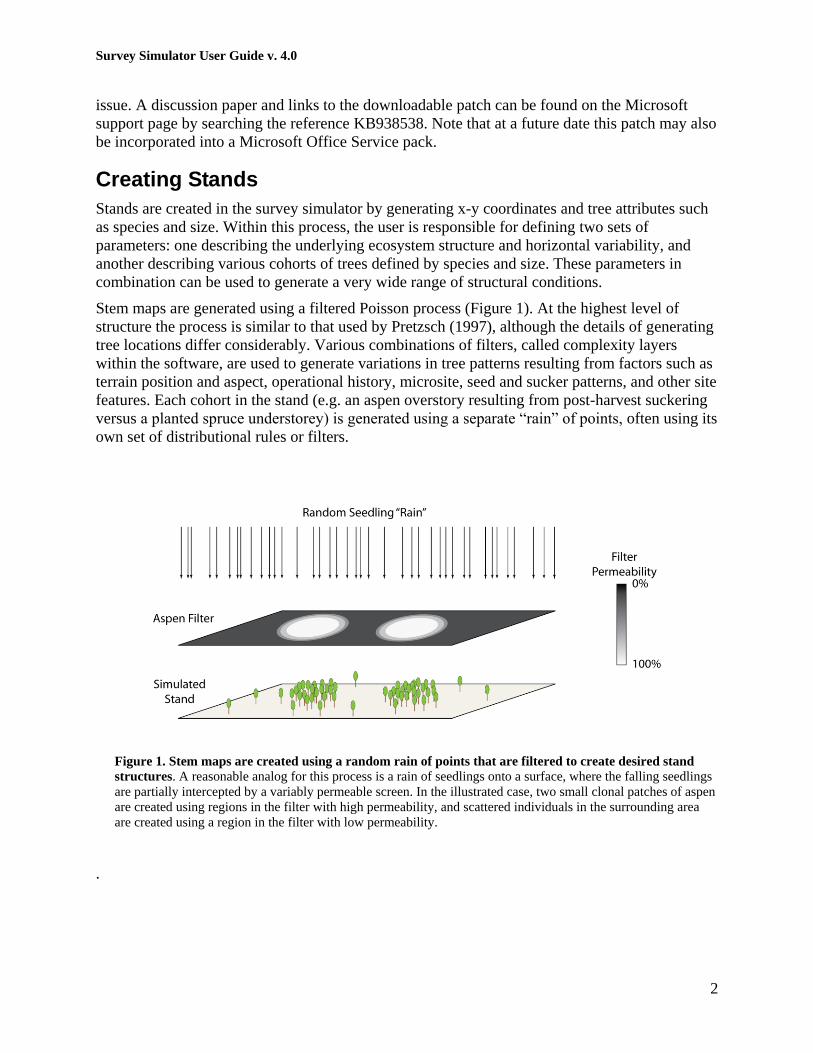
Stem maps are generated using a filtered Poisson process (Figure 1). At the highest level of

structure the process is similar to that used by Pretzsch (1997), although the details of generating

tree locations differ considerably. Various combinations of filters, called complexity layers

within the software, are used to generate variations in tree patterns resulting from factors such as

terrain position and aspect, operational history, microsite, seed and sucker patterns, and other site

features. Each cohort in the stand (e.g. an aspen overstory resulting from post-harvest suckering

versus a planted spruce understorey) is generated using a separate “rain” of points, often using its

own set of distributional rules or filters.

Figure 1. Stem maps are created using a random rain of points that are filtered to create desired stand

structures. A reasonable analog for this process is a rain of seedlings onto a surface, where the falling seedlings

are partially intercepted by a variably permeable screen. In the illustrated case, two small clonal patches of aspen

are created using regions in the filter with high permeability, and scattered individuals in the surrounding area

are created using a region in the filter with low permeability.

.


3

Horizontal Complexity Layers

To generate stem maps that reflect species and spatial diversity at a cutblock scale, 7 layers of

information are utilized, each reflecting a different pattern or scale of variation:

1. Terrain Position

Terrain position is the primary layer of information underlying all others and is used to

control the influence of all others. Terrain positions are mapped using Voronoi polygons

(Figure 2). Points representing terrain summits within the stem map and a 200 m

surround are assigned randomly or at user selected positions. Polygon boundaries

representing valleys or draws are defined using lines whose points are equidistant to the

nearest two summit points.

Figure 2. Voronoi polygons as the basis for terrain units.

Voronoi polygons are based on random points within the stem mapped area (dashed line) and

a surrounding zone of influence. Red dots (polygon centroids) represent terrain summits, and

polygon boundaries (lines for which all points are equidistant to the two nearest centroids)

represent valleys (troughs) between.

Figure 3. Derivation of Terrain positions.

Within a Voronoi polygon, any radius can be subdivided to generated concentric zones

reflecting terrain position (left), based on user defined radial percentages. The result is a

zonation of the stem map (right), where points representing tree locations are colour

coded by terrain position.

Polygon centroid = meso-terrain summit

Polygon boundary = meso-terrain trough

1

2

3

4 5

6

Terrain positions


4

Voronoi polygons can be further subdivided to reflect slope position (Figure 3). Any point

within a polygon can be classified based on the relative radial distance from the summit to the

polygon boundary. Six terrain positions are recognized. While this zonation is intended to

mimic the classification of crest, upper, mid, lower, toe and depressional slope positions, it

can also be used for other purposes such as defining large scale clusters of trees with

graduated edges.

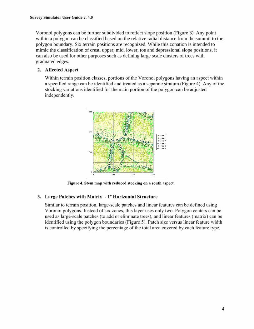
2. Affected Aspect

Within terrain position classes, portions of the Voronoi polygons having an aspect within

a specified range can be identified and treated as a separate stratum (Figure 4). Any of the

stocking variations identified for the main portion of the polygon can be adjusted

independently.

Figure 4. Stem map with reduced stocking on a south aspect.

3. Large Patches with Matrix - 1º Horizontal Structure

Similar to terrain position, large-scale patches and linear features can be defined using

Voronoi polygons. Instead of six zones, this layer uses only two. Polygon centers can be

used as large-scale patches (to add or eliminate trees), and linear features (matrix) can be

identified using the polygon boundaries (Figure 5). Patch size versus linear feature width

is controlled by specifying the percentage of the total area covered by each feature type.


5

Figure 5. Stem map illustrating use of Voronoi polygons to define linear features.

In this case, the linear features have a different stand composition than the

remainder of the stand. Note that parameters can be specified such that effects of

linear features on composition can be varied by terrain position.

4. Large Discrete Patches - 2º Horizontal Structure

Similar to terrain position and the large patches with matrix, large discrete patches are

generated using Voronoi polygons. In this case, however, once the polygons have been

divided into two zones, only the central zone is utilized. The result is a set of discrete

patches (Figure 6) that are non-overlapping. Large patches are defined based on a mean

number of centers in a 10 ha area and the percentage of the total area covered.

Figure 6. Use of large patches for spatial diversity.

Large patches can be superimposed over a stem map, and trees added or

subtracted by species. In this case, the dense clumps might represent clonal

aspen patches in a conifer plantation. If desired, the occurence of one species

can be reduced while another is increased.


6

5. Small Scale Patches (3 layers) - 3º Horizontal Structure

Small-scale patches are circular units with randomly located centers. Patch radii are

drawn from a truncated normal distribution with the mean and standard deviation

specified by the user, and tails cut off at +/- 3 standard deviations. These patches are used

to add and/or subtract trees from a simulated stand to create spatial diversity (Figure 7).

Within each of the 3 small-scale layers, patches can overlap, but the effects of overlap

within a discrete layer are not additive.

0

100

200

300

0 100 200 300

Posit ion 1

Posit ion 2

Posit ion 3

Posit ion 4

Posit ion 5

Posit ion 6

0

100

200

300

0 100 200 300

Posit ion 1

Posit ion 2

Posit ion 3

Posit ion 4

Posit ion 5

Posit ion 6

Figure 7. Use of small-scale patches for spatial diversity.

Randomly spaced trees (left) have been re-arranged (right) to create small-scale spatial

diversity. In this case, trees removed from one set of patches were replaced in another set

with different random centers.

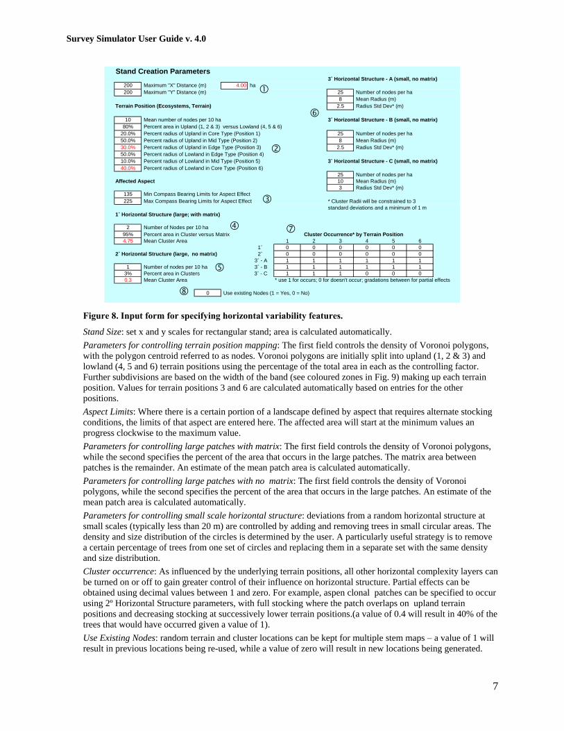
The seven horizontal complexity layers are controlled through an input form on an Excel

worksheet (Figure 8). Included on this form are entries to specify cutblock size, relative area

occupied by each terrain position, definition of the “affected aspect”, and size/distribution of the

various horizontal structure features. A final segment of the form (lower right) allows the effect

of any of the horizontal structure layers to be partially or wholly attenuated by terrain position

(i.e. if 4000 trees/ha are added to the stand in large discrete patches, this can be reduced to a

lower number on lower slopes and in depressions to reflect poorer suckering success on wetter

sites).


7

Figure 8. Input form for specifying horizontal variability features.

Stand Size: set x and y scales for rectangular stand; area is calculated automatically.

Parameters for controlling terrain position mapping: The first field controls the density of Voronoi polygons,

with the polygon centroid referred to as nodes. Voronoi polygons are initially split into upland (1, 2 & 3) and

lowland (4, 5 and 6) terrain positions using the percentage of the total area in each as the controlling factor.

Further subdivisions are based on the width of the band (see coloured zones in Fig. 9) making up each terrain

position. Values for terrain positions 3 and 6 are calculated automatically based on entries for the other

positions.

Aspect Limits: Where there is a certain portion of a landscape defined by aspect that requires alternate stocking

conditions, the limits of that aspect are entered here. The affected area will start at the minimum values an

progress clockwise to the maximum value.

Parameters for controlling large patches with matrix: The first field controls the density of Voronoi polygons,

while the second specifies the percent of the area that occurs in the large patches. The matrix area between

patches is the remainder. An estimate of the mean patch area is calculated automatically.

Parameters for controlling large patches with no matrix: The first field controls the density of Voronoi

polygons, while the second specifies the percent of the area that occurs in the large patches. An estimate of the

mean patch area is calculated automatically.

Parameters for controlling small scale horizontal structure: deviations from a random horizontal structure at

small scales (typically less than 20 m) are controlled by adding and removing trees in small circular areas. The

density and size distribution of the circles is determined by the user. A particularly useful strategy is to remove

a certain percentage of trees from one set of circles and replacing them in a separate set with the same density

and size distribution.

Cluster occurrence: As influenced by the underlying terrain positions, all other horizontal complexity layers can

be turned on or off to gain greater control of their influence on horizontal structure. Partial effects can be

obtained using decimal values between 1 and zero. For example, aspen clonal patches can be specified to occur

using 2º Horizontal Structure parameters, with full stocking where the patch overlaps on upland terrain

positions and decreasing stocking at successively lower terrain positions.(a value of 0.4 will result in 40% of the

trees that would have occurred given a value of 1).

Use Existing Nodes: random terrain and cluster locations can be kept for multiple stem maps – a value of 1 will

result in previous locations being re-used, while a value of zero will result in new locations being generated.

Stand Creation Parameters3˚ Horizontal Structure - A (small, no matrix)

200 Maximum "X" Distance (m) 4.00 ha

200 Maximum "Y" Distance (m) 25 Number of nodes per ha

8 Mean Radius (m)

Terrain Position (Ecosystems, Terrain) 2.5 Radius Std Dev* (m)

10 Mean number of nodes per 10 ha 3˚ Horizontal Structure - B (small, no matrix)

80% Percent area in Upland (1, 2 & 3) versus Lowland (4, 5 & 6)

20.0% Percent radius of Upland in Core Type (Position 1) 25 Number of nodes per ha

50.0% Percent radius of Upland in Mid Type (Position 2) 8 Mean Radius (m)

30.0% Percent radius of Upland in Edge Type (Position 3) 2.5 Radius Std Dev* (m)

50.0% Percent radius of Lowland in Edge Type (Position 4)

10.0% Percent radius of Lowland in Mid Type (Position 5) 3˚ Horizontal Structure - C (small, no matrix)

40.0% Percent radius of Lowland in Core Type (Position 6)

25 Number of nodes per ha

Affected Aspect 10 Mean Radius (m)

3 Radius Std Dev* (m)

135 Min Compass Bearing Limits for Aspect Effect

225 Max Compass Bearing Limits for Aspect Effect

1˚ Horizontal Structure (large; with matrix)

2 Number of Nodes per 10 ha

95% Percent area in Cluster versus Matrix Cluster Occurrence* by Terrain Position

4.75 Mean Cluster Area 1 2 3 4 5 6

1˚ 0 0 0 0 0 0

2˚ Horizontal Structure (large, no matrix) 2˚ 0 0 0 0 0 0

3˚ - A 1 1 1 1 1 1

1 Number of nodes per 10 ha 3˚ - B 1 1 1 1 1 1

3% Percent area in Clusters 3˚ - C 1 1 1 0 0 0

0.3 Mean Cluster Area * use 1 for occurs; 0 for doesn't occur; gradations between for partial effects

0 Use existing Nodes (1 = Yes, 0 = No)

* Cluster Radii will be constrained to 3

standard deviations and a minimum of 1 m


8

Vertical Structure and Species Composition

Species composition and vertical structure are also controlled through a series of input forms.

Separate forms are used to specify planted or other layers with a semi-regular distribution

(Figure 9) versus those with a random or clumped distribution (Figure 10) typical of natural

regeneration. In both cases, ten records (rows) are available, which can be used either for

different species, different species specifications in different terrain positions and/or different

layers or cohorts within a species. For multiple layers, more than one row can be used for each

species with different tree size, density and spatial criteria.

For planted trees, the entire stand is assumed to be planted to the same density, and is

apportioned by species using percentages by terrain position and aspect. Adjustments to density

due to mortality can be specified in a random pattern by terrain position or in a clumped pattern

using complexity layers.

For natural trees, density is specified as trees/ha by species, terrain position and aspect, and is

initially specified by terrain position and aspect. Further adjustments are made by adding or

subtracting trees by terrain position, aspect and/or complexity layers.


9

Planted Trees

1200 Total Number of Planted Trees per Hectare

20% Spacing Tolerance (percent of mean inter-tree distance)

Species Mean StdDev 1 2 3 4 5 6 1 2 3 4 5 6

101 SW 1 3 0.59 50% 50% 50% 80% 80% 80% 20% 20% 20% 80% 80% 80% 9 6

102 PL 1 4.3 0.42 40% 50% 50% 20% 20% 20% 80% 80% 80% 20% 20% 20% 9 4

103

104

105

106

107

108

109

110

Total: 100% 100% 100% 100% 100% 100% 100% 100% 100% 100% 100% 100%

2 Number of Species

Species 1 2 3 4 5 6 1 2 3 4 5 6 (1=Yes, 0=No)

101 SW 5% 5% 5% 5% 5% 5% 5% 5% 5% 5% 5% 5% 0% 0% 0% 0% 0% 0% 1

102 PL 10% 10% 10% 10% 10% 10% 0% 0% 0% 0% 0% 0% 0% 0% 0% 0% 0% 0% 1

103 0

104 0

105 0

106 0

107 0

108 0

109 0

110 0

Age

Best

Years to

BH

Height affected by

overtopping cohorts?3˚ - C

Clusters

Random Mortality by Terrain Position (%) Random Mortality by Terrain Position Within Affected Aspect (%)1˚

Clusters

1˚

Matrix

3˚ - A

Clusters

3˚ - B

Clusters

Additional Random Mortality By:

2˚

Clusters

Preference

Code

Height

Percent of Total Trees by Terrain Position Within Affected Aspect

(each column must sum to 100%)

Percent of Total Trees by Terrian Position

(each column must sum to 100%)

Figure 9. Input form for planted trees with regular spacing.

Each row in this table represents a different stand cohort, broke down primarily by species but potentially also by

size or age. It is assumed that the same total density (trees/ha as specified in top left corner) will be initially

established throughout the stem map, but that species composition and post-planting mortality can vary based on

various combinations of horizontal complexity layers.

Species: Any species codes as a text string can be used; codes will be carried through to the tree list and survey

reports.

Preference Code: This is a numerical value intended for use in silviculture surveys to allow preferential selection of

one species over another where two adjacent trees can be selected for a stocking assessment and reporting of overall

species composition by stocking.

Height: For each layer, specify the mean height and a standard deviation. Height distributions are assumed to be

normal.

Percent of Total Trees by Terrain Position (and Aspect): Species composition of planted trees must be specified

separately for each combination of terrain position and aspect class. In the example above, the species composition

is 50% white spruce (SW) and 50% lodgepole pine (PL) for terrain position 1 over most of the area, but changes to

20% spruce and 80% pine on the “affected” aspect. Each column in this section must sum to 100%.

Age and Best Years To Breast Height: The age for each layer should include the age of trees at the time of planting

(e.g. 2-year old seedling + 8 years since planting = 10 years). Best years to breast height is the total age of the tallest

seedlings upon reaching a height of 1.3 m assuming no overtopping suppression.

Random Mortality by Terrain Position: Mortality expected to have occurred from the time of planting to the current

age of the simulated stand must be specified separately for each combination of terrain position and aspect class. In

the example above, 5% of the spruce and 10% of the pine is expected to have dies over most of terrain position 1,

switching to no pine mortality in the “affected aspect”.

Additional Random Mortality by Cluster Type: Mortality in addition to that specified by terrain position can be

specified for each of the 1º, 2º, and 3º horizontal complexity layers. For planted trees, this section can be used to

generate effects such as losses in stocking due to unstockable areas (e.g. rock and swamp), intense competition from

brush patches or root diseases. It can also be used in situations where planting would not have occurred in the

presence of patches of advance regeneration. In this latter case, the „mortality‟ for the planted trees would be 100%,

and the same horizontal complexity layer would also be used within the “Stand - Natural Trees” worksheet to create

the advance regeneration.

Height Affected by Overtopping Cohorts? : Where the height growth of planted trees is likely to be affected by

patches of overtopping trees from other layers, such effects can be triggered by entering a value of 1 for the

appropriate layer in this section. Correspondingly, calibration parameters for a height reduction model will also be

required (see Appendix 2).


10

Natural Trees

Species Mean StdDev 1 2 3 4 5 6 1 2 3 4 5 6

201 AT 1 3.5 0.5 10000 10000 10000 7000 5000 4000 10000 10000 10000 7000 5000 4000

202 AC 1 3.7 0.5 500 500 500 1000 2000 2000 500 500 500 1000 2000 2000

203

204

205

206

207

208

209

210

Total 10500 10500 10500 8000 7000 6000 10500 10500 10500 8000 7000 6000

2 Number of Species

Additional Trees By:

(% of original number by terrain position)

Species Min Max (1=Yes, 0=No)

201 AT 0% 0% 0% 70% 0% 0% 0% 0% 70% 0% 6 10 4 0

202 AC 0% 0% 0% 70% 0% 0% 0% 0% 70% 0% 6 10 4 0

203 0

204 0

205 0

206 0

207 0

208 0

209 0

210 0

Height affected by

overtopping

cohorts?3˚ - B

Clusters

Percentage Stand Density Decrease By:

3˚ - C

Clusters

3˚ - C

Clusters

1˚

Clusters

2˚

Clusters

3˚ - A

Clusters

3˚ - B

Clusters

Age

Total trees/ha by Terrain Position Due to AspectHeightPreference

Code

1˚

Matrix

2˚

Clusters

3˚ - A

Clusters

Total Trees/ha by Terrain Position

(distribution but not numbers adjusted by lower level clusters)

Best Yrs

to BH

Figure 10. Input form for naturally regenerated trees with variations on a random distribution.

Each row in this table represents a different stand component, broke down primarily by species but also by size or

age. Unlike the situation for planted trees, the density is not constant across all terrain positions and aspect classes,

but instead is the sum of the values specified for each layer.

Species: Any species codes as a text string can be used; codes will be carried through to the tree list and survey

reports.

Preference Code: This is a numerical value intended for use in silviculture surveys to allow preferential selection of

one species over another where two adjacent trees can be selected for a stocking assessment and reporting of overall

species composition by stocking.

Height: For each layer, specify the mean height and a standard deviation. Height distributions are assumed to be

normal.

Total Trees by Terrain Position (and Aspect): Species composition of natural trees must be specified separately for

each combination of terrain position and aspect class. In the example above, the overall density (trees/ha) declines

from upland terrain positions moving to the wetter lowland terrain positions. At the same time, the prevalence of

aspen (AT) declines while the prevalence of cottonwood (AC) increases. Also in this example, there is no change

specified by aspect class. Also in this example, there is no change specified by aspect class. Also in this example,

there is no change specified by aspect class.

Percentage Stand Density Decrease By Cluster Type: The initial stand density specified by terrain position and

aspect class can be altered based on overlaps with the horizontal structure features. For example, a narrow matrix for

the 1º horizontal structure clusters can be used to simulate reduced natural regeneration on skid trails.

Additional Trees By Cluster Type: The initial stand densities specified by terrain position and aspect class can also

be augmented based on overlap with horizontal complexity features. This ability is useful for creating discrete

patches of natural regeneration. It is also extremely useful in combination with „Decreases By Cluster Type‟ for

creating fine scale (< 10 m) clustering. In the example illustrated above, 70% of the trees are removed from one set

of 3º clusters and replaced in a second set. Such re-arrangement of trees from the initial Poisson distribution can be

used to create a large degree of variability in spatial pattern, although considerable trial and error may be required to

get the desired results.

Age and Best Years To Breast Height: Specify the maximum and minimum ages that might be measured for trees in

a particular layer, and the age of the fastest growing trees upon reaching a height of 1.3 m assuming no overtopping

suppression.

Height Affected by Overtopping Cohorts? : Where the height growth of trees is likely to be affected by patches of

overtopping trees from other layers, such effects can be triggered by entering a value of 1 for the appropriate layer in

this section. Correspondingly, calibration parameters for a height reduction model will also be required (see

Appendix 2).


11

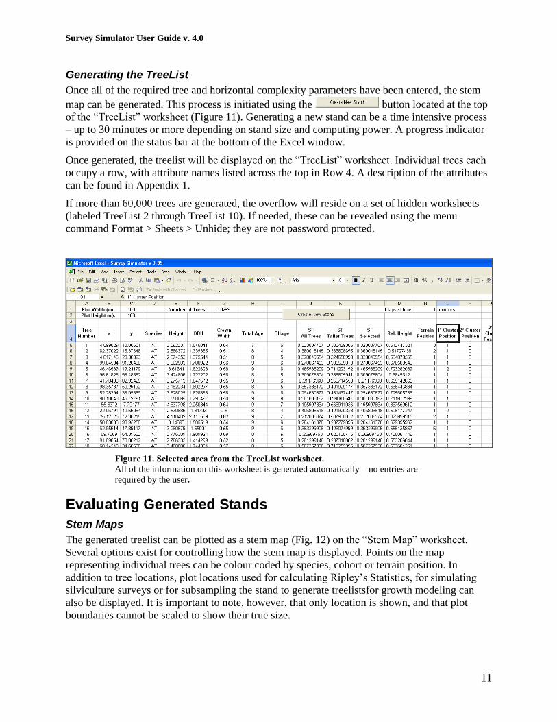
Generating the TreeList

Once all of the required tree and horizontal complexity parameters have been entered, the stem

map can be generated. This process is initiated using the button located at the top

of the “TreeList” worksheet (Figure 11). Generating a new stand can be a time intensive process

– up to 30 minutes or more depending on stand size and computing power. A progress indicator

is provided on the status bar at the bottom of the Excel window.

Once generated, the treelist will be displayed on the “TreeList” worksheet. Individual trees each

occupy a row, with attribute names listed across the top in Row 4. A description of the attributes

can be found in Appendix 1.

If more than 60,000 trees are generated, the overflow will reside on a set of hidden worksheets

(labeled TreeList 2 through TreeList 10). If needed, these can be revealed using the menu

command Format > Sheets > Unhide; they are not password protected.

Figure 11. Selected area from the TreeList worksheet.

All of the information on this worksheet is generated automatically – no entries are

required by the user.

Evaluating Generated Stands

Stem Maps

The generated treelist can be plotted as a stem map (Fig. 12) on the “Stem Map” worksheet.

Several options exist for controlling how the stem map is displayed. Points on the map

representing individual trees can be colour coded by species, cohort or terrain position. In

addition to tree locations, plot locations used for calculating Ripley‟s Statistics, for simulating

silviculture surveys or for subsampling the stand to generate treelistsfor growth modeling can

also be displayed. It is important to note, however, that only location is shown, and that plot

boundaries cannot be scaled to show their true size.


12

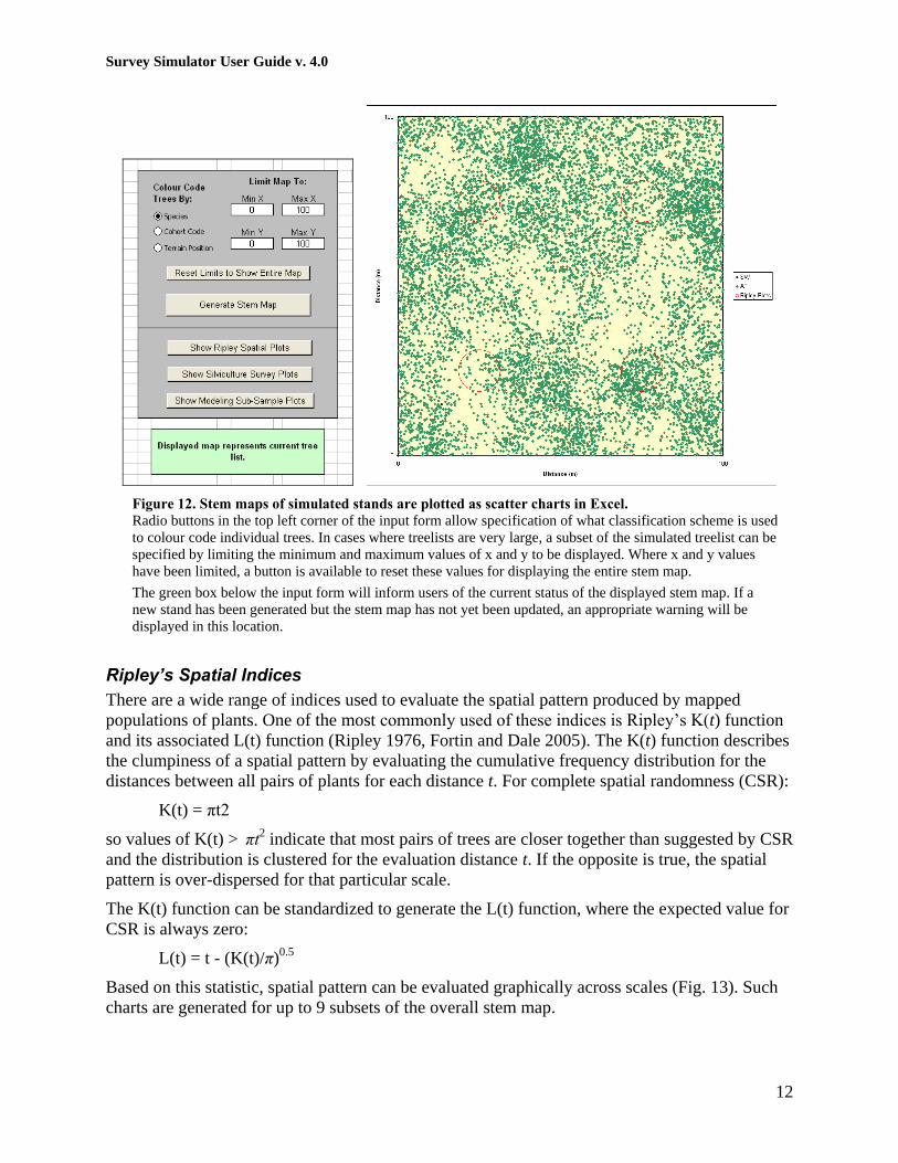
Figure 12. Stem maps of simulated stands are plotted as scatter charts in Excel.

Radio buttons in the top left corner of the input form allow specification of what classification scheme is used

to colour code individual trees. In cases where treelists are very large, a subset of the simulated treelist can be

specified by limiting the minimum and maximum values of x and y to be displayed. Where x and y values

have been limited, a button is available to reset these values for displaying the entire stem map.

The green box below the input form will inform users of the current status of the displayed stem map. If a

new stand has been generated but the stem map has not yet been updated, an appropriate warning will be

displayed in this location.

Ripley’s Spatial Indices

There are a wide range of indices used to evaluate the spatial pattern produced by mapped

populations of plants. One of the most commonly used of these indices is Ripley‟s K(t) function

and its associated L(t) function (Ripley 1976, Fortin and Dale 2005). The K(t) function describes

the clumpiness of a spatial pattern by evaluating the cumulative frequency distribution for the

distances between all pairs of plants for each distance t. For complete spatial randomness (CSR):

K(t) = πt2

so values of K(t) > πt

2 indicate that most pairs of trees are closer together than suggested by CSR

and the distribution is clustered for the evaluation distance t. If the opposite is true, the spatial

pattern is over-dispersed for that particular scale.

The K(t) function can be standardized to generate the L(t) function, where the expected value for

CSR is always zero:

L(t) = t - (K(t)/π)0.5

Based on this statistic, spatial pattern can be evaluated graphically across scales (Fig. 13). Such

charts are generated for up to 9 subsets of the overall stem map.


13

-1

-0.5

0

0.5

1

0 5 10 15

t

L(t

)

-1

-0.5

0

0.5

1

0 5 10 15

t

L(t

)

The Ripley spatial statistics and the L(t) charts are found on a worksheet labeled “Ripley Stats”.

The top left corner of this sheet contains input forms and control buttons for generating the

statistics and charts (Fig. 14).

Caution: Generating spatial statistics is a slow process – expect to wait anywhere from

several minutes to half an hour, depending on the number of sub-samples, the sub-sample

radius and the processor speed of your computer.

Further information on Ripley‟s statistics is available from a number of sources including Ripley

(1976), Diggle (1983), Dale (1999), Fortin and Dale (2005).

Figure 13. Examples of L(t) functions.

In the top chart, trees are overdispersed

(more evenly spaced than would be

expected with CSR) at scales less than 1

m, possibly due to self-thinning. At

scales from 1 to 12 m, the stand is

clustered, and becomes overdispersed

again for larger scales. In the bottom

chart, the stand is overdispersed at scales

out to 9, a pattern that would be typically

of regularly spaced plantations. The

clustering at larger scales might indicate

large unstockable gaps or patches of

mortality in the plantation.


14

Sample Design Grid

Number of Plots 4

No. Plots - x Direction 2

No. Plots - y Direction 2

Plot Radius (m) 25

Note: The L(t) charts follow a convention whereby

K(t) is subtracted from the expected value given

complete spatial randomness. Values of L(t) greater

than zero indicate overdispersion, while values less

than zero indicate clumpiness at the given scale of

evaluation (x-axis in metres).

Dispayed L(t) charts represent the current stand

Generate Ripley's K Statistics

-1

-0.5

0

0.5

1

0 5 10 15

t

L(t

)

-1

-0.5

0

0.5

1

0 5 10 15

t

L(t

)

Spacing Factor

In some cases, the relative frequency of sample points with different values for spacing factor

may provide a good indication of spatial variability or, more particularly, thedistribution of

competitive environments within a stand. From a silviculture perspective, spacing factor can be

used to indicate locations where trees are excessively crowded for achieving a given set of

management objectives versus other areas that are within a desired range or are understocked. In

boreal mixed stands of juvenile aspen and spruce, for example, spruce growing below an aspen

canopy starts to lose height increment below spacing factors of approximately 0.25 (C. Farnden,

unpublished data). To provide an estimate of the distribution of competitive conditions within

simulated stands, two distribution charts are provided in Figure 15.

Figure 14. Input form for Ripley’s Statistics.

Ripley‟s statistics in this usage are based on samples

of the population using circular plots. Plots can be

randomly located or arranged on a grid, with up to 9

samples per stand. Users need to enter the sample

design (grid versus random), the number of sample

plots (1 to 9), the number of plots in the x direction

(grid systems only), and the sample plot radius. For

grid systems, the number of plots in the y direction

will be calculated automatically, and the total number

of plots specified must be evenly divisible by the

number of plots in the x direction. The plot radius

should be at least 20 m.

The top green box below the input form will inform

users of the current status of the displayed charts. If a

new stand has been generated but the L(t) charts have

not yet been updated, an appropriate warning will be

displayed in this location.

The bottom green box reminds users that there are two

different conventions for calculating L(t) statistics,

and indicates which variation has been used in this

case.


15

0

10

20

30

40

50

60

<0.1 0.1 to

0.2

0.2 to

0.3

0.3 to

0.4

0.4 to

0.5

0.5 to

0.6

0.6 to

0.7

0.7 to

0.8

0.8 to

0.9

> 0.9

Spacing Factor

Rela

tive F

req

uen

cy (

%)

0

10

20

30

40

50

60

70

80

90

100

0 0.1 0.2 0.3 0.4 0.5 0.6 0.7 0.8 0.9 1

Spacing Factor

Cu

mu

lati

ve F

req

uen

cy (

%)

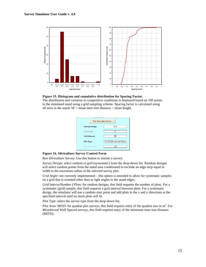
Figure 15. Histogram and cumulative distribution for Spacing Factor.

The distribution and variation in competitive conditions is displayed based on 100 points

in the simulated stand using a grid sampling scheme. Spacing factor is calculated using

all trees in the stand: SF = mean inter-tree distance ÷ mean height.

Figure 16. Silviculture Survey Control Form

Run Silviculture Survey: Use this button to initiate a survey.

Survey Design: select random or grid (systematic) from the drop-down list. Random designs

will select random points from the stand area conditioned to exclude an edge strip equal in

width to the maximum radius of the selected survey plot.

Grid Angle: not currently implemented – this option is intended to allow for systematic samples

on a grid that is oriented other than at right angles to the stand edges.

Grid Interva/Number f Plots: for random designs, this field requests the number of plots. For a

systematic (grid) sample, this field requests a grid interval between plots. For a systematic

design, the simulator will use a random start point and add plots in the x and y directions at the

specified interval until no more plots will fit.

Plot Type: select the survey type from the drop-down list.

Plot Area/ MITD: for quadrat plot surveys, this field requires entry of the quadrat size in m2. For

Mixedwood Well Spaced surveys, this field requires entry of the minimum inter-tree distance

(MITD).


16

Surveys

Silviculture surveys are run from the “Survey” worksheet using an input form (Fig 16). Three

survey methods designed for use in boreal mixedwood stands are currently implemented:

1. 5-5-2-2 (Boreal Mixedwood Survey)

The 5-5-2-2 survey starts with a 50 m2 plot that is divided into quadrants (BC Ministry of

Forests 2009, page 112 to 117; variant of survey for macro, meso and micro-scale patched

mixedwoods), each of which is roughly analogous to a stocked quadrat plot. Each quadrant

is evaluated as being either unstocked, stocked with broadleaved trees (aspen or

cottonwood), stocked with spruce or stocked with both broadleaves and spruce. In order for

a spruce to be tallied, a further assessment is required using a tree-centered subplot. The

subplot is again divided into quadrants, and the spruce must be free of broadleaved

competition for a distance of at least 5 m in two quadrants and 2 m in the remaining

quadrants in order for the spruce tree to be “well growing” and tallied.

In the BC MoF version of this survey, the subplot quadrants with a competition-free radius

of 5 m must be adjacent. In its original version and that implemented in the simulator, the 5

m radii need not be in adjacent quadrants.

Summary statistics for this survey are comprised of the percentage of plot quadrants that

fall within each of the four stocking categories.

2. Stocked Quadrats

Stocked quadrat surveys use small fixed area plots (or quadrats) each of which represents a

sample of potentially occupiable growing space. Each quadrat is tallied as being unstocked,

stocked with broadleaved trees, stocked with spruce, or stocked with both broadleaves and

spruce. There is no fixed plot size for the quadrats – plot area can be set by the user.

Summary statistics for this survey are comprised of the percentage of quadrats that fall

within each of the four stocking categories, as for quadrants in the 5-5-2-2.

3. Mixedwood Well-Spaced

The mixedwood well-spaced survey uses an extension of the standard well spaced survey

procedure (BC Ministry of Forests 2009, pages 23 to 27) utilized for a high percentage of

regenerating stands in BC. In the mixedwood variation used here, three separate tallies of

well-spaced trees are required:

Well-spaced spruce, using a minimum inter-tree distance of 2 m, ignoring the

presence of broad-leaved trees

Well-spaced deciduous trees (aspen and cottonwood), ignoring the presence of

spruce

Total well spaced trees, ignoring the concept of species

In each tally, tree selections are made to maximize the number of well spaced trees; for the

final tally of total trees this will usually require selection of different trees than were chosen

for the species specific tallies.


17

The tally of total well spaced trees is intended to primarily capture the total usage of growing

space (or inversely, what percentage in unoccupied). The species specific tallies help to

apportion that growing space between the spruce and broadleaves.

Summary statistics for this survey include: 1) mean number of total well-spaced trees, 2)

mean number of broadleaved well-spaced trees, 3) mean number of spruce well-spaced trees

and 4) mean number of aspen well spaced trees associated with each well spaced spruce:

n

i

n

i

p

j

n

p

C

SwperAtMean

1

1 1

This last statistic is intended as a measure of the mean level of competition experienced by the

spruce in the stand imposed by the overtopping broadleaved trees.

Survey summary statistics are displayed on the “Survey” worksheet (Fig. 17), while individual

plot outcomes can be found on a hidden worksheet labeled “Survey Outcomes”. The outcomes

worksheet is hidden simply to avoid clutter and is not password protected.

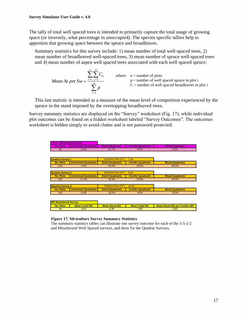
No. Plots Unstocked Quadrants Decid Quadrants Conifer Quadrants Mixed Quadrants

36 8.3% 91.7% 0.0% 0.0%

Quadrat Survey 1 Quadrat Area (m2): 7.50


100 4.0% 25.0% 13.0% 58.0%



100 17.0% 36.0% 13.0% 34.0%



100 0.0% 16.0% 9.0% 75.0%

WS Mixedwood Survey

No. Plots Mean Conif WS Mean Decid WS Mean Total WS Mean Decid WS per Conifer WS

49 5.63 6.49 7.88 5.60

5-5-2-2 Mixedwood Survey

Figure 17. Silviculture Survey Summary Statistics

The summary statistics tables can illustrate one survey outcome for each of the 5-5-2-2

and Mixedwood Well Spaced surveys, and three for the Quadrat Surveys.

where: n = number of plots

p = number of well spaced spruce in plot i

C = number of well spaced broadleaves in plot i


18

TreeLists For Growth Models

Currently, treelists can be generated only for the MGM growth model. Treelist generation is

controlled from the data entry form (Fig. 18) on the “Growth Modeling” worksheet.

Figure 18. Growth Model TreeList Control Form

Growth Model: Use this button to initiate a survey.

Survey Design: select random or grid (systematic) from the drop-down list. Random designs

will select random points from the stand area conditioned to exclude an edge strip equal in

width to the maximum radius of the selected survey plot.

Grid Angle: not currently implemented – this option is intended to allow for systematic samples

on a grid that is oriented other than at right angles to the stand edges.

Grid Interva/Number f Plots: for random designs, this field requests the number of plots. For a

systematic (grid) sample, this field requests a grid interval between plots. For a systematic

design, the simulator will use a random start point and add plots in the x and y directions at the

specified interval until no more plots will fit.

Plot Area: area of the sample plots (m2) used to generate individual treelists. The plot needs to

be large enough to capture 10 to 50 locally competing trees. The plot should be small enough

that it represents a relatively uniform set of competitive conditions within the stand. A plot area

of 100 m2 is a good place to start.

MGM works best with a treelist that is at lest 30 to 40 trees. If a smaller treelist is created at a

particular sample location, it will be multiplied to generate addition tree records until at least 40

trees are present. The plot expansion factors are automatically adjusted so that the stand level

values represented by the plot (e.g. trees/ha) are accurately retained.

Treelist files created in this manner are placed in a user defined directory. A form is provided on

the “Growth Modeling” worksheet, where the user can select either the same directory as the

survey simulator workbook, or browse for any other directory.


19

References

BC Ministry of Forests, 2009. Silviculture Survey Procedures Manual.

http://www.for.gov.bc.ca/hfp/publications/00099/Surveys/Silviculture%20Survey%20Pro

cedures%20Manual-April%201%202009.pdf, accessed March 29, 2009.

Dale, M.R.T. 1999. Spatial pattern analysis in plant ecology. Cambridge University Press,

Cambridge UK.

Diggle, P.J. 1983. Statistical analysis of point patterns. Academic Press, London UK.

Fortin, M-J and Dale, M. 2005, Spatial analysis, a guide for ecologists. Cambridge University

Press, Cambridge UK.

Pretzsch, H. 1997. Analysis and modeling of spatial stand structures. Methodological

considerations based on mixed beech-larch stands in Lower Saxony. Forest Ecology and

Management, 97: 237-253.

http://www.for.gov.bc.ca/hfp/publications/00099/Surveys/Silviculture%20Survey%20Procedures%20Manual-April%201%202009.pdf

http://www.for.gov.bc.ca/hfp/publications/00099/Surveys/Silviculture%20Survey%20Procedures%20Manual-April%201%202009.pdf


20

Appendix 1. Tree Attributes

In order of column number, the following attributes are provided on the “TreeList” worksheet:

Tree Number: A unique numerical account for each tree.

X: Horizontal distance of the tree from the left margin of the stand.

Y: Vertical distance of the tree from the bottom edge of the stand.

Species: An alphanumeric code, specified by the user, to indicate discrete species.

Height: Tree height in metres. An initial height is randomly drawn from a normal distribution

where the mean and standard deviation are specified by the user. Where necessary, height is

adjusted downward to reflect the effects of overtopping competition (see Appendix 2)

DBH: Bole diameter in centimetres measured at a height of 1.3 m from the ground. Diameter is

calculated as a function of height and spacing factor (see Appendix 2).

Crown Width: Mean radial diameter of the tree crown in metres. Currently, crown width is

generated as a crude linear function of DBH (CW = 0.31 + 0.148*DBH). Crown width has been

included as an attribute to facilitate its use in surveys where it is needed to evaluate of

overtopping competition.

Total Age: Years since germination. For planted trees, age is specified by the user. For natural

trees, age is initially estimated as a function of height, and adjusted based on a random draw

from a skewed beta distribution (see Appendix 2).

BHage: Breast Height Age is the number of years since reaching a height of 1.3 m; also

described as the ring count of a tree cored with an increment borer at a height of 1.3 m. This

value is calculated as a function of height and total age, assuming a linear fit between height and

age for trees above breast height (see Appendix 2).

SF All Trees: Spacing Factor (mean inter-tree distance as a percentage of mean height)

calculated using all trees within a calculated search radius of the subject tree. The search radius

is determined as 70% of the maximum tree height in the stand.

SF Taller Trees: Spacing Factor (mean inter-tree distance as a percentage of mean height)

calculated using all trees taller than the subject tree within a calculated search radius of the

subject tree. The search radius is determined as 70% of the maximum tree height in the stand.

SF Selected: Spacing Factor (mean inter-tree distance as a percentage of mean height) calculated

using all trees of user selected species set within a calculated search radius of the subject tree.

The search radius is determined as 70% of the maximum tree height in the stand.

Relative Height: Height of the subject tree as a proportion of the height of the maximum

potential height a given cohort.

Terrain Position: Record of terrain position associated with subject tree. Possible values are

integers 1 through 6.

1˚ Cluster Position: Record of position within primary horizontal complexity layer – value of 1

represents cluster, value of 2 represents matrix.


21

2˚ and 3˚ Cluster Positions: Records of position within secondary and tertiary clusters. A value

of 1 indicates tree is within a given cluster set, a value of 0 indicates tree is not within a given

cluster set.

Affected Aspect: Record of position within affected aspect. A value of 1 indicates tree lies

within the aspect range defined as the “affected aspect”, while a value of 0 indicates that it lies

outside that range.

Nearest Cluster & X & Y: Number and x-y coordinates of nearest terrain position centroid to

the subject tree.

2nd

Nearest Cluster & X & Y: Number and x-y coordinates of second nearest terrain position

centroid to the subject tree.

Survey Preference Code: Ranking factor provided by the user in the specification of stand

cohorts to indicate a preference of one species over another when choosing trees for stocking

assessments in silviculture surveys.

Competition Map Pixel: Parameter used to subset the stem map into small grid squares for

evaluation of local competition. Pixel dimensions are based on rounding up the spacing factor

search radius to the nearest integer than divides evenly into the x and y stand dimensions

respectively. A cluster of 9 pixels centered on the one containing the subject tree will then

contain all possible trees needed to assess local competition. A similar process is used to subset

the stand for survey plots and plots used to generate treelists for initiating growth model

simulations (where pixel size is based on rounding up the plot radius).

Cohort/Layer: Record of the cohort from which a particular tree was derived, as specified by

the user.


22

Appendix 2: Sub-Models

Tree Height Adjustments

Tree heights are initially drawn from a normal distribution with mean and standard deviation

specified by the user (see Figures 9 and 10 in main text). Where height is anticipated to have

been affected by overtopping competition by trees from other cohorts1, height can be adjusted

downward using a multiplier (range = 0 to 1). The multiplier is determined as a function of one

of three variations on spacing factor, using one of eight different functional shapes and using

calibration parameters as set by the user. An example of a function for the impact of an aspen

canopy on understorey spruce is illustrated in Figure 2-1.

Built-in functions available to represent this type of relationship include:

Weibull: 3211

bxb

eby

where b1 is fixed at 1.00

Chapman Richards: 3211

bxbeby

where b1 is fixed at 1.00

Generalized Logistic: xbb

eb

by

32

4

1

where b1 = b4 = 1.00

Gompertz: xbb

eeby32

1

where b1 = 1.00

Segmented Linear: 12 by for x > b1

)( 132 xbbby for x < b1

Specifying the function to use along with the appropriate parameters is done using a form in

columns X through AH of the „Stand Creation Parameters‟ worksheet (Fig. 2-2).

1 Cohorts needing adjustment must be indicated on the cohort description forms – see Figures 9 & 10.

Figure 2-1. Weibull fit of relative spruce height as

predicted by spacing factor calculated using the

overtopping deciduous canopy. Relative spruce

height was determined by first fitting the curve

using absolute spruce height, then dividing each

height value by the asymptote.

228.32.3771 xey

RMSE = 0.19


23

Height Adjustment Parameters

Cohort Model Code b1 b2 b3 b4 b5

Model Form* Model Code 101 1 1 377.2 3.2278 0 0

Weibull (3 param) 1 102 1 1 377.2 3.2278 0 0

Chapman-Richards 2 103 1 1 377.2 3.2278 0 0

Gen. Logistic 3 104 1 1 377.2 3.2278 0 0

Gompertz 4 105 1 1 377.2 3.2278 0 0

Segmented Linear 5 106 1 1 377.2 3.2278 0 0

Polynomial 6 107 1 1 377.2 3.2278 0 0

Exp Polynomial* 7 108 1 1 377.2 3.2278 0 0

Linear 8 109 1 1 377.2 3.2278 0 0

* Hover cursor over model name for format 110 1 1 377.2 3.2278 0 0

Measure of Competition Used in Predictions: 201 1 0 0 0 0 0

Spacing Factor 1 202 1 0 0 0 0 0

Spacing Factor Taller 2 203 1 0 0 0 0 0

Spacing Factor Selected Cohorts 3 204 1 0 0 0 0 0

205 1 0 0 0 0 0

Ht Adj Model Uses: 3 206 1 0 0 0 0 0

DBH Model Uses: 3 207 1 0 0 0 0 0

208 1 0 0 0 0 0

209 1 0 0 0 0 0

210 1 0 0 0 0 0

Calibrated Models:

Planted white spruce under aspen (Farnden 2009)

1 1 377.2 3.2278 0 0

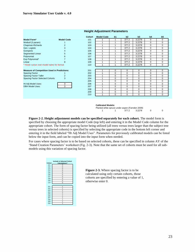
Figure 2-2. Height adjustment models can be specified separately for each cohort. The model form is

specified by choosing the appropriate model Code (top left) and entering it in the Model Code column for the

appropriate cohort. The form of spacing factor being utilized (all trees versus trees larger than the subject tree

versus trees in selected cohorts) is specified by selecting the appropriate code in the bottom left corner and

entering it in the field labeled “Ht Adj Model Uses”. Parameters for previously calibrated models can be listed

below the input form, and can be copied into the input form when needed.

For cases where spacing factor is to be based on selected cohorts, these can be specified in column AY of the

„Stand Creation Parameters‟ worksheet (Fig. 2-3). Note that the same set of cohorts must be used for all sub-

models using this variation of spacing factor.

Cohort

101 0

102 0

103 0

104 0

105 0

106 0

107 0

108 0

109 0

110 0

201 1

202 1

203 1

204 1

205 1

206 1

207 1

208 1

209 1

210 1

Include in Selected Cohort

Calculations?

Figure 2-3. Where spacing factor is to be

calculated using only certain cohorts, those

cohorts are specified by entering a value of 1,

otherwise enter 0.


24

Diameter

Diameters are calculated as a function of height (Fig 2-4). Separate diameter versus height

functions can be utilized for each cohort.

A number of functional forms are available including:

Weibull: 3211

bxb

eby

Chapman Richards: 3211

bxbeby

Generalized Logistic: xbb

eb

by

32

4

1

Gompertz: xbb

eeby32

1

Polynomial: 4

5

3

4

2

321 xbxbxbxbby

Exponential Polynomial: 4

5

3

4

2

321)log( xbxbxbxbby

Linear: xbby 21

Specifying the function to use along with the appropriate parameters is done using a form in

columns X, Y and AK through AU of the „Stand Creation Parameters‟ worksheet (Fig. 2-2).

Figure 2-4. Linear fit of logarithmically

transformed dbh for aspen diameters predicted by

height.

xey 2797.04106.0

I2 = 0.87

RMSE = 0.67


25

Diameter Prediction Parameters

Cohort Model Code b1 b2 b3 b4 b5 b6 b7 b8 b9

Model Form* Model Code 101 8 -1.503 1.4193 0 0 0

Weibull (3 param) 1 102 8 -1.503 1.4193 0 0 0

Chapman-Richards 2 103 8 -1.503 1.4193 0 0 0

Gen. Logistic 3 104 8 -1.503 1.4193 0 0 0

Gompertz 4 105 8 -1.503 1.4193 0 0 0

Segmented Linear 5 106 8 -1.503 1.4193 0 0 0

Polynomial 6 107 8 -1.503 1.4193 0 0 0

Exp Polynomial* 7 108 8 -1.503 1.4193 0 0 0

Linear 8 109 8 -1.503 1.4193 0 0 0

* Hover cursor over model name for format 110 8 -1.503 1.4193 0 0 0

Measure of Competition Used in Predictions: 201 7 -0.416 0.2797 0 0 0

Spacing Factor 1 202 7 -0.416 0.2797 0 0 0

Spacing Factor Taller 2 203 7 -0.416 0.2797 0 0 0

Spacing Factor Selected Cohorts 3 204 7 -0.416 0.2797 0 0 0

205 7 -0.416 0.2797 0 0 0

Ht Adj Model Uses: 3 206 7 -0.416 0.2797 0 0 0

DBH Model Uses: 3 207 7 -0.416 0.2797 0 0 0

208 7 -0.416 0.2797 0 0 0

209 7 -0.416 0.2797 0 0 0

210

Calibrated Models:

Planted white spruce under aspen (Farnden 2009)

8 -1.503 1.4193 0 0 0

Aspen - natural sucker stand (Farnden 2009)

7 -0.4106 0.2797 0 0 0

Figure 2-4. Diameter models can be specified separately for each cohort. The model form is specified by choosing

the appropriate model Code (columns X & Y at left) and entering it in the Model Code column for the appropriate

cohort. The form of spacing factor being utilized (all trees versus trees larger than the subject tree versus trees in

selected cohorts) is specified by selecting the appropriate code in the bottom left corner and entering it in the field

labeled “DBH Model Uses”. Parameters for previously calibrated models can be listed below the input form, and

can be copied into the input form when needed. Columns for parameters b6 through b9 are not currently used, but

have been provided to allow for future inclusion of random variation.

For cases where spacing factor is to be based on selected cohorts, these can be specified in column AY of the „Stand

Creation Parameters‟ worksheet (Fig. 2-3). Note that the same set of cohorts must be used for all sub-models using

this variation of spacing factor.

Cohort

101 0

102 0

103 0

104 0

105 0

106 0

107 0

108 0

109 0

110 0

201 1

202 1

203 1

204 1

205 1

206 1

207 1

208 1

209 1

210 1

Include in Selected Cohort

Calculations?

Figure 2-3. Where spacing factor is to be

calculated using only certain cohorts, those

cohorts are specified by entering a value of 1,

otherwise enter 0.


26

Total Age

Total age for natural trees is calculated primarily as a function of height, assuming that the oldest

trees are also most likely to be the tallest. The first step, then, is to interpolate age from height:

minminmax

minmax

min )()(

)(AgeAgeAge

HeightHeight

HeightHeightAgeinitial

where Heightmax, Heightmin, Agemax and Agemin are determined as 3 standard deviations from the

mean for a normal distribution as specified by the user (see Figures 9 and 10 in the main text).

The next step adjusts this linear distribution upward to generate a distribution that is skewed to

older ages (assuming that more trees germinate earlier rather than later, and that older trees are

more likely to have survived early stages of self-thinning). Adjustments are based on random

draws from a skewed cumulative beta distribution (Fig. 2-5), such that most trees get a relatively

small adjustment, but a few are quite large:

)( max initialdrawinitialfinal AgeAgeBetaAgeAge

0

0.2

0.4

0.6

0.8

1

0 0.2 0.4 0.6 0.8 1

Random Value

Cu

mu

lati

ve

Be

ta(1

.5,4

)

Figure 2-5. Cumulative beta distribution

where alpha = 1.5 and beta = 4. Based on a

uniform random value, a draw is made from

the cumulative distribution to obtain and

adjustment factor for total age.


27

Breast Height Age

Breast height age is calculated from total age and height, assuming that the relationship between

height and age for young trees is linear above breast height. Breast height age is then calculated

as:

)()3.1(

xTotalBH InterceptAgeHeight

HeightAge

where interceptx is the x intercept of the linear fit for the age versus height relationship above

breast height (Fig. 2-6).

0

1

2

3

4

5

0 5 10 15

Age (yrs)

He

igh

t (m

)

1.3 m

Total Age

Years to BH

AgeBH

Figure 2-6. AgeBH determination utilizes the

assumption that a height versus age

relationship (red line) is close to linear (black

dashed line) above breast height for young

trees.


28

Appendix 3: Batch Runs

The simulator contains no built-in routine for batch runs. It has, however, been constructed to

facilitate batch runs. Some knowledge of the VBA programming language is required. There are

three steps to the process:

1. Build an excel worksheet containing the parameters that need to be changed in each

successive run of the simulator, with one row for each simulation and a run ID number or

name in the first cell.

2. Construct a VBA macro that will copy the parameters into the appropriate locations on

the simulator worksheets, run the simulator, and save the results. In pseusdo-code:

Sub Batch_Macro()

For i = 1 to Number_Of_Simulations

Copy parameters from Row i of batch workbook to simulator, where

the first column contains a Run ID

Call the appropriate simulator subroutine(s)

Save the simulator workbook using the Run ID from cell (i,1)

Next i

End Sub

The simulator workbook must be open before the batch run is started, and should not be

closed between successive simulations.

Subroutines that may need to be called to initiate batch runs include:

Create_Stand2 Equivalent to selecting the “Create New Stand” button on the

“TreeList” worksheet.

Run_Survey Equivalent to selecting the “Run Silviculture Survey” button on

the “Survey” worksheet.

Run_Modeling_TreeLists Equivalent to selecting the “Generate TreeLists For Growth

Models” button on the “TreeList” worksheet

Generate_Map Equivalent to selecting the “Generate Stem Map” button on the

“Stem Map” worksheet

Generate_Spatial_Stats Equivalent to selecting the “Generate Ripley‟s K Statistics”

button on the “Ripley Stats” worksheet


29

Appendix 4: Coding New Surveys

In order to code in a new survey methodology there are several actions that you need to take with

regard to worksheet locations in the simulator workbook:

1. Add the survey name to the Plot Type list in Column BA of the “Survey” worksheet.

2. Ensure that the Data Validation option for cell D10 on the “Survey” worksheet covers the

range of cells that includes your entry in Column BA.

3. Determine the number of statistics that need to be recorded for each plot in the survey.

4. Unhide the Sheet labeled “Survey Outcomes” and identify a range of unused columns

that is sufficiently wide enough to encompass all of your plot level statistics plus Plot

Number, X-coordinate and y-coordinate (see examples already present on this

worksheet). Label your columns. Note that this worksheet has been set up with many

blank columns between successive survey methods to allow for future adjustments.

5. Create a block of cells on the “Survey” worksheet (starting in column G) to summarize

the plot level statistics from the “Survey Outcomes” worksheet into stand level statistics

as desired. Use Excel formulas to sum, average or otherwise compile the plot level

statistics into stand level statistics.

6. Determine user defined plot variables (such as plot area or minimum inter-tree distance

for well spaced trees) and assign then to input fields in the user form on the top left

corner of the “Survey” worksheet. In doing so, note that:

The first four fields (rows 4, 6, 8 and 10) should not be changed

The fifth field (row 12) can be used for any purpose, and the field label set to

change (via a cell formula) according to the choice made for Plot Type (row 10).

Additional fields can be added below the current ones as needed.

The next step is to develop an algorithm for your survey and translate it into VBA code. All code

for silviculture surveys is found in Module 1, and follows the flow chart illustrated in Figure 4-1.


30

Sub Survey_Design

• Read in survey parameters

• Create plot centers

Sub Read_TreeList

• Read in stem map from

Excel worksheet

• Create subsets of treelist

by grid squares (pixels)

Sub Create_Plot_TreeList

• Compile subset of main treelist

specific tp plot

Various Survey Subroutines

• Determine which trees are “in”

• Compile plot statistics into array

Call appropriate survey

subroutine

Write plot statistics to

“Survey Outcomes”

worksheet

Count

Through plots:

More required?

Start

End

Yes

No

Sub Survey_Design

• Read in survey parameters


Sub Read_TreeList

• Read in stem map from

Excel worksheet

• Create subsets of treelist

by grid squares (pixels)

Sub Create_Plot_TreeList

• Compile subset of main treelist

specific tp plot

Various Survey Subroutines

• Determine which trees are “in”

• Compile plot statistics into array

Call appropriate survey

subroutine

Write plot statistics to

“Survey Outcomes”

worksheet

Count

Through plots:

More required?

Count

Through plots:

More required?

Start

End

Yes

No

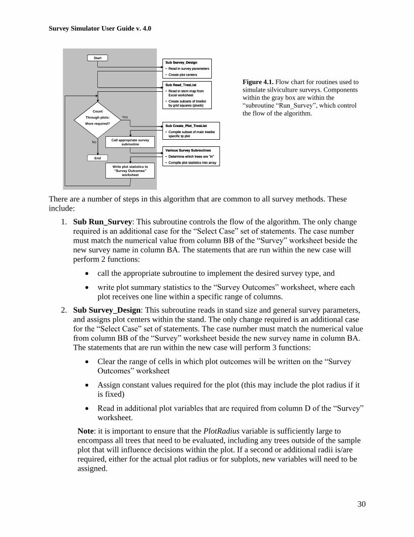
There are a number of steps in this algorithm that are common to all survey methods. These

include:

1. Sub Run_Survey: This subroutine controls the flow of the algorithm. The only change

required is an additional case for the “Select Case” set of statements. The case number

must match the numerical value from column BB of the “Survey” worksheet beside the

new survey name in column BA. The statements that are run within the new case will

perform 2 functions:

call the appropriate subroutine to implement the desired survey type, and

write plot summary statistics to the “Survey Outcomes” worksheet, where each

plot receives one line within a specific range of columns.

2. Sub Survey_Design: This subroutine reads in stand size and general survey parameters,

and assigns plot centers within the stand. The only change required is an additional case

for the “Select Case” set of statements. The case number must match the numerical value

from column BB of the “Survey” worksheet beside the new survey name in column BA.

The statements that are run within the new case will perform 3 functions:

Clear the range of cells in which plot outcomes will be written on the “Survey

Outcomes” worksheet

Assign constant values required for the plot (this may include the plot radius if it

is fixed)

Read in additional plot variables that are required from column D of the “Survey”

worksheet.

Note: it is important to ensure that the PlotRadius variable is sufficiently large to

encompass all trees that need to be evaluated, including any trees outside of the sample

plot that will influence decisions within the plot. If a second or additional radii is/are

required, either for the actual plot radius or for subplots, new variables will need to be

assigned.

Figure 4.1. Flow chart for routines used to

simulate silviculture surveys. Components

within the gray box are within the

“subroutine “Run_Survey”, which control

the flow of the algorithm.


31

3. Sub Read_TreeList: This subroutine reads the treelist for the entire stand and subdivides

it into grid rectangles (or pixels). The dimensions of each pixel are as small as possible

such that the x and y dimensions are larger than the value of the PlotRadius variable, and

will divide evenly into the respective x and y stand dimensions (MaxX and MaxY

variables). Each pixel is assigned a vector within a 2-D array which contains a list of all

trees that occur within that pixel. No changes are required in this subroutine.

4. Sub Create_Plot_TreeList: This subroutine finds the pixel that contains a plot center

along with the eight surrounding pixels to form a 3 x 3 grid of pixels. The list of trees in

each of the nine pixels is then used to compile a new treelist that is a subset of the main

treelist and contains all of the trees that need to be evaluated for a given plot. No changes

are required in this subroutine.

The remaining subroutines in Module 1 are unique to specific surveys, and are called from the

Run_Survey subroutine as required. These subroutines are called separately for each plot. The

data available to be used by the survey method subroutines include:

a) A 2-D array labeled PlotTrees containing all trees to be evaluated in the plot. Each row in

the array is an individual tree, and each column is an attribute as described in Appendix

1. The order of attributes is the same as can be found on the “TreeList” worksheet.

b) A set of variables including PlotRadius and any other variables or constants that are

specific to the plot type.

Also available are a set of built in functions which can be found in Module 3. Of particular

interest is a function that calculates the distance between two points:

Dist(x1, y1 ,x2 ,y2)

The new survey subroutine should calculate plot level statistics (e.g. stocking class, count of

trees by species, count of well spaced trees by species) based on rules imposed by the survey

methodology, with the statistics stored as variables that are accessible in the Run_Survey

subroutine.


32

Appendix 5: Coding New Modeling TreeLists

In order to code in a new sub-sampling methodology for creating tree-lists to initial simulations

in accessory growth and yield models, there are several actions that you need to take with regard

to worksheet locations in the simulator workbook:

1. Add the survey name to the Plot Type list in Column BI of the “Growth Modeling”

worksheet.

2. Ensure that the Data Validation option for cell E5 on the “Growth Modeling” worksheet

covers the range of cells that includes your new entry in Column BI.

3. Ensure that the user form in the top left corner of the “Growth Modeling” worksheet

contains all of the require plot parameters.. In doing so, note that:

The first four fields (rows 4, 6, 8 and 10) should not be changed

The fifth field (row 12) can be used for any purpose, and the field label set to

change (via a cell formula) according to the choice made for Growth Model

(row 5).

Additional fields can be added below the current ones as needed. For instance,

if a nested plot is required, additional plot radii or basal area factors may be

required.

The next step is to develop an algorithm for your sampling scheme and translate it into VBA

code. All code for growth model sub-sampling is found in Module 5, and follows the flow chart

illustrated in Figure 5-1.

Sub Model_Plots

• Read in sample design parameters


Sub Read_TreeList_For_Models

• Read in stem map from Excel

worksheet

• Create subsets of treelist by grid

squares (pixels)

Create subset treelist from

pixels

Determine which tree ar “in” the

sample plot

Count

Through plots:

More required?

Count

Through plots:

More required?

Start

End

Yes

No

Determine for which models to

create treelists

Various Subroutines

- Start -

Write trees to output file with:

• Any required additional attributes

• Appropriate column order

• Appropriate header information


33

There are a number of steps in this algorithm that need either no change or minimal change for

adding new modeling methods. These include:

1. Sub Run_Modeling_TreeLists: This subroutine controls the flow of the algorithm. The

only change required is an additional case for the Select Case set of statements. The case

number must match the numerical value from column BJ of the “Survey” worksheet

beside the new survey name in column BI. The only statement that is run from the Select

Case set of statements is a call to another subroutine that contains algorithms for defining

the contents of the sub-sample treelist.

2. Model_Plots: This subroutine reads in stand size and general sub-sampling parameters,

and assigns plot centers within the stand. The only change that may be required is the

addition of statements to read in any additional plot parameters that may have been

added. These statements are near the top of the subroutine following a comment that

reads Read in Survey Design Parameters.

Note: The variable PlotRadius is calculated from a user defined plot area.

3. Sub Read_TreeList_For_Models: This subroutine reads the treelist for the entire stand

and subdivides it into grid rectangles (or pixels). The dimensions of each pixel are as

small as possible such that the x and y dimensions are larger than the value of the

PlotRadius variable, and will divide evenly into the respective x and y stand dimensions

(MaxX and MaxY variables). Each pixel is assigned a vector within a 2-D array which

contains a list of all trees that occur within that pixel. No changes are required in this

subroutine.

There is also a block of code identified in the Create_MGM_TreeList subroutine that will be

required for each new sample algorithm. This block of code creates a subset of the main treelist

that covers a mapped area slightly larger than each sample plot.

The remaining subroutines in Module 5 are unique to specific surveys, and are called from the

Run_Modeling_TreeLists subroutine as required. For MGM, there is a main subroutine called

Create_MGM_Stands that controls the flow and output, and a second routine called

Create_MGM_TreeList that carries out instruction specific to individual sample plots. The

functions of these routines include:

1. Count through the desired number of sample plots

2. Read in a subset of the main treelist specific to each plot

3. Create a 2-D array containing trees from the subset are in the sample plot

4. Write the 2_D array to a new file, with a column order suited to the specific model‟s

input requirements, alon with any other required formatting and header requirements.

The data available to be used by the sampling subroutines include:

1. A 2-D array labeled PlotTrees containing all trees to be evaluated in the plot. Each row in

the array is an individual tree, and each column is an attribute as described in

Appendix 1. The order of attributes is the same as can be found on the “TreeList”

worksheet.

2. A set of variables including PlotRadius and any other variables or constants defined

earlier that are specific to the plot type.


34

Also available are a set of built in functions which can be found in Module 3. Of particular

interest is a function that calculates the distance between two points:

Dist(x1, y1 ,x2 ,y2)

craig farnden - british columbia farnden, march 2009. survey simulator user guide v. 4.0 ii table of...

Documents