craniometry of the equidae part i: two-dimensional … · 07.05.2018 · f:am 60823 pliohippus...

Paludicola 7(1):1-13 October 2008 © by the Rochester Institute of Vertebrate Paleontology

1

CRANIOMETRY OF THE EQUIDAE PART I: TWO-DIMENSIONAL SHAPE ANALYSIS

Robert L. Evander

Department of Vertebrate Paleontology, American Museum of Natural History, Central Park West at 79th, New York NY 10024

ABSTRACT Morphometric analysis of landmark data on fifty-three drawings of fossil horse skulls reveals that the first principal component of horse skull shape variation involves a simultaneous decrease in the relative size of the braincase, an increase in the relative size of the maxilla, an increase in the relative length of the malar crest, a deepening of the nasal incisure, and the movement anteriorly and inferiorly of the maxillary alveoli relative to the orbit and braincase. Two other principal components of shape variation also emerge. These results identify the Frick collection of fossil skull illustrations as an important graphic database of fossil mammal form.

INTRODUCTION

One particular advantage of studying the fossil horses of the Frick Collection is a portfolio of extraordinary illustrations. These illustrations were drawn by a succession of artists employed by Childs Frick to illustrate his collection. The longest serving of these artists were Hazel DeBerard (retired 1958) and Raymond Gooris (retired about 1985). Although none of the illustrations are signed or dated, it is likely that the choice of specimens was made by Morris Skinner during the 1960's, and that the bulk of these illustrations are therefore the artwork of Raymond Gooris. The Frick fossil horse portfolio includes approximately 350 line drawings, mostly of horse dentitions. Significantly for this study, the Frick portfolio also includes fifty-two lateral aspects of relatively complete mature horse skulls. When Frick artists illustrated a specimen of the size of a horse skull, they began by outlining the principal features using a suspension pantograph. Two of these instruments survive at the American Museum of Natural History, where they were transferred as part of the donation of the Frick Collection. A suspension pantograph is simply a large pantograph in which the various linkages of the instrument are suspended from a central tower. The suspension mechanism allows for large excursions by both the stylus and the pen of the pantograph; and at the same time allows nimble movements of the heavy, solid metal arms of the instrument. This large excursion was necessary because all of the fossil horse illustrations share a scale of 1:1. That is, all of the illustrations are drawn to the actual size of the specimen. To enable the positioning of these large specimens, the Frick Laboratory had a special lift

constructed. Only a couple of feet square, this lift allowed the positioning of the specimen just below the stylus of the pantograph and just off the table upon which the artwork was positioned. The pantograph produces an image that is in zero-point perspective in artistic terminology, or that is a parallel projection in mathematical terminology. This means that x-y coordinates of features on the illustrations are accurate records of their x-y coordinates in two-dimensional space. Thus, because Childs Frick dictated a correct choice of illustration techniques 70 years ago, we have a portfolio of 50-year-old horse illustrations that are amenable to morphometric analysis by the most modern of analytical techniques.

PROCEDURE

The fifty-two illustrations (Table 1) were scanned into Adobe Photoshop as grayscale images at 600 dpi using an Epson 1640XL large-format flatbed scanner in the Microscope and Imaging Facility at the American Museum. Five of the illustrations proved too large for the bed of the scanner. These five illustrations were scanned in two parts, and the parts merged using Adobe Photoshop. Because my primary intent at the time of the scanning was the creation of a computer portfolio of publication-ready illustrations, all of the figures were rotated to a uniform orientation and scaled to a bed size of 14.5 centimeters. These orientation and scale manipulations were performed using Adobe Photoshop. The original 600 dpi image density was maintained. The electronic files were converted from Photoshop documents (.psd) to JPEG images (.jpg) using Adobe Photoshop. Each of the images occupied roughly 1,000

PALUDICOLA, VOL. 7, NO. 1, 2008

2

TABLE 1 - The skulls analyzed. “<>” indicates holotype specimen. Number Identity Locality Figure 7 AMNH 1752 Equus andium Punin ECUADOR 1 F:AM 60009 Equus sp. Cripple Creek AK 2 F:AM 60028 Equus sp. Cripple Creek AK 3 F:AM 60030 Equus sp. Fairbanks Creek AK 4 F:AM 60351 Protohippus perditus Devil's Gulch Horse Quarry NB 5 F:AM 60500 Hypohippus sp. Xmas Quarry NB 6 F:AM 60700 Megahippus matthewi Plum Creek NB 7 F:AM 60775 Sinohippus zitteli Ma Chi Lien Kou CHINA 8 F:AM 60810 Pliohippus mirabilis Devil's Gulch Horse Quarry NB 9 F:AM 60812 Pliohippus mirabilis Pole Creek NB 10 F:AM 60823 Pliohippus mirabilis Devil's Gulch Horse Quarry NB 11 F:AM 69500 "Merychippus" coloradense Chama-el Rito NM 12 F:AM 69503 "Merychippus" coloradense Canyada Moquino NM 13 F:AM 69506 "Merychippus" coloradense Uhl Pit CO 14 F:AM 69508 "Merychippus" sp. Paleo-channel Quarry NB 15 F:AM 69511 "Merychippus" coloradense Boulder Quarry NB 16 F:AM 69550 "Merychippus" sp. Trinity River Pit I TX 17 F:AM 69700 "Merychippus" primus Greenside Quarry NB 18 F:AM 69701 "Merychippus" primus Greenside Quarry NB 19 F:AM 71000 "Merychippus" sp. Mill Quarry NB 20 F:AM 71018 "Merychippus" sp. East Sand Quarry NB 21 F:AM 71154 "Merychippus" cf. isonesus East Sand Quarry NB 22 F:AM 71700 Parahippus cognatus Sand Canyon NB 23 F:AM 71800 Cormohipparion occidentale Xmas Quarry NB 24 F:AM 71887 Hipparion forcei Olcott Quarry NB 25 F:AM 71888 Cormohipparion quinni <> Devil's Gulch Horse Quarry NB 26 F:AM 73909 Cormohipparion skinneri <> Gidley's Horse Quarry TX 27 F:AM 73940 Cormohipparion goorisi <> Trinity River Pit I TX 28 F:AM 74023 Mesohippus bairdii NW of Conata SD 29 F:AM 74400 Hipparion tehonense MacAdams Quarry TX 30 F:AM 87001 Merychippus insignis Echo Quarry NB 31 F:AM 87001 Merychippus insignis Echo Quarry NB 32 F:AM 87201 Dinohippus interpolatus Edson Quarry KS 33 F:AM 87301 Scaphohippus intermontanus East Sand Quarry NB 34 F:AM 108644 Neohipparion affine Leptarctus Quarry NB 35 F:AM 108645 Calippus martini MacAdams Quarry TX 36 F:AM 109909 Hipparion brevidontus Trinity River Pit I TX 37 F:AM 110128 Parapliohippus carrizoensis Yermo Quarry CA 38 F:AM 111728 Neohipparion affine MacAdams Quarry TX 39 F:AM 114730 Neohipparion affine near Big Spring Quarry CO 40 F:AM 116128 Protohippus perditus Paleo-channel Quarry NB 41 F:AM 126899 "Merychippus" sp. Deep Creek NB 42 F:AM 128154 "Merychippus" calamarius Tesuque NM, near 43 F:AM 141219 Cormohipparion merriami <> June Quarry NB 44 F:AM 142498 Parahippus tyleri Dunlap Camel Quarry NB 45 F:AM 142511 "Merychippus" primus Hilltop Quarry NB 46 F:AM 142515 "Merychippus" sp. Boulder Quarry NB 47 F:AM 142647 Scaphohippus intermontanus Skull Ridge NB 48 F:AM 142648 Scaphohippus intermontanus Skull Ridge NB 49 UNSM 1159 "Merychippus" sp. Railway Quarry 'A' NB 50 UNSM 1352 Cormohipparion goorisi Railway Quarry 'A' NB 51 UNSM 1353 Hypohippus affinis Gordon Creek Quarry NB 52

EVANDER—CRANIOMETRY OF THE EQUIDAE

3

KB of disk space. The 600 dpi resolution was not affected by the conversion to JPEGs. These images were then processed into digitizing software (Rohlf, 2005) downloaded from the Stony Brook Morphometrics site (http://life.bio.sunysb.edu/morph/). The tpsDig software version 2.10 allows simple manipulations of the image (magnification control, frame changes) so that landmarks can be placed precisely at the cursor with the click of the mouse. Thirty-three landmarks were located on each of the images using tpsDig (Figure 1, Table 2). The program labels and numbers each of the landmarks on the illustration, and thus provides a graphic resume of the digitizing process. But the essential output from the tpsDig is an x-y location for each of the thirty-three landmarks recorded in the units of pixels which output as a .tps file. The x-y locations reported out of the tpsDig software were then treated by the Morphologika2 software version 2.4 (O’Higgins and Jones, 2006) downloaded from the Morphologika site (http: //hyms.fme.googlepages.com/downloadmorphologika). The tpsDig output required minor reformatting to become Morphologika2 input. (The latest version of Morphologika2 accepts tpsDig output directly.) Shape analysis by Morphologika2 proceeds by three steps: a preliminary generalized Procrustes analysis, and unseen transformation of the Procrustes results into an abstract mathematical method for the description of shape, then a principal components analysis performed on data twice transformed. These steps require a few paragraphs of explanation, as only two steps are clearly visible to a user. Generalized Procrustes analysis is a mathematically rigorous method for aligning the landmarks from two (or more) specimens as neatly as possible. The Procrustes analysis employed by Morphologika2 (O’Higgins and Jones, 1998) requires three steps: calculation of location of the centroid for each specimen, size normalization of all the specimens, and registration of all the specimens. A centroid, effectively the mean landmark taking all landmarks into consideration, is calculated for each specimen in the analysis. The x coordinate of the centroid is the average of all the x coordinates of the landmarks for that specimen, and the y coordinate is the average of all the y coordinates (Figure 2). Size normalization involves calculating centroid size for each specimen, defined as the square root of the sum of the squared distances from the centroid to each of the landmarks (Figure 3) (O’Higgins and Jones, 1998). For each specimen, every landmark is then divided by that specimen’s centroid size, resulting in a new set of size-adjusted landmarks where geometry is preserved. Finally, the various specimens are superimposed by aligning the centroids all specimens, and rotating one specimen about the centroid until the sum of distances

between analogous landmarks are minimized (Figure 4). This process of rotating for the minimum difference in distances is known as registration. _____________________________________________ TABLE 2. The landmarks analyzed.

Description 1 Most anterior spur of bone between the alveoli of the two I1's 2 Intersection of the alveolar border of the premaxilla with the canine 3 Intersection of the alveolar border of the maxilla with the canine 4 Intersection of the alveolar border of the maxilla with the P3 5 Highest point of bone above the incisors 6 Maximum perpendicular distance from a line connecting landmarks 5 and 7 7 Deepest point of the nasal notch 8 Highest point on the rim of the orbit 9 Most anterior point on the rim of the orbit 10 Lowest point on the rim of the orbit 11 Most posterior point on the rim of the orbit 12 Most anterior point on the rim of the temporal fossa 13 Center of the rim of the infraorbital foramen 14 Intersection of the maxillary tuberosity with the M3 alveolus 15 Most posterior bone of the nuchal crest 16 Crest of the occipital condyles 17 Intersection of the basisphenoid and the basipterygoid 18 Most anterior point on the nasals 19 Point on the top of the skull just above landmark 7 20 Point on the top of the skull just above landmark 20 21 Highest point on the skull 22 Anterior limit of the malar crest 23 Lowest point on the bottom of the zygomatic arch 24 Highest point on the bottom of the zygomatic arch 25 Lowest point on the articular condyle of the zygomatic arch 26 Deepest point in the condylar fossa 27 Tip of the postglenoid process 28 Most anterior point in the incisure at the posterior attachment of the zygomatic arch 29 Most posterior point on the zygomatic arch 30 Highest point on the top of the zygomatic arch 31 Highest point on the crest of the temporal fossa 32 Lowest point on the top of the zygomatic arch 33 Most posterior point on the rim of the lacrimal fossa ________________________________________________________ Output from the Procrustes analysis consists of a transformed set of x-y coordinates for the thirty-three landmarks. The transformed coordinates are geometrically similar to the original coordinates because they preserve the same shape. The transformed coordinates preserve the geometric relationships between all landmarks. The transformed coordinates may show significant rotations from the original coordinates, but in this case the rotations are subtle because the original coordinates had been visually aligned during the scanning process. The transformed coordinates are not congruent with the original coordinates because they have been adjusted for size. The original coordinates could be measured in pixels scanned at 600 dpi. Because of the size changes, the transformed coordinates are dimensionless distances.


4

FIGURE 1: The thirty-three landmarks. ______________________________________________________________________________________________________________________________

FIGURE 2: Calculating the location of the centroid. The thirty-three landmarks are shown in the upper left. In the upper right, the average of the thirty-three x coordinates is calculated. (Only four of the thirty-three x coordinates are shown as contributing to the calculation.) In the lower left, the average of the thirty-three y coordinates is calculated. (Again, only four of the thirty-three y coordinates are shown as contributing to the calculation.) In the lower right average of the x coordinates and the average of the y coordinates are the (x,y) coordinates of the centroid. __________________________________________________________________________________________________________________________

FIGURE 3: Calculating the size of the centroid. Lines are drawn from the centroid to each of the thirty-three landmark points. The length of each of the lines is calculated, those lengths are squared, and the squares summed. The size of the centroid is the square root of the sum of the squares.


5

When operating the Morphologika2 program, the Procrustes analysis is readily apparent to the user, as he or she clicks on a pull down menu item to initiate the Procrustes analysis. The principal components analysis at the end of the program similarly is evoked clicking on another pull down menu item. But between this first and this final step, a full-fledged data conversion occurs, and this conversion is transparent to the user. Perhaps this transparency is best, because it involves quite a leap into mathematical abstraction. On the other hand, it appears that the great power of this software is due to this unseen leap into difficult mathematical concepts. Morphologika2 does not analyze the landmark coordinates themselves. It analyses the relative position of the landmarks to each other. In Morphologika2, the principal components analysis is performed in Kendall’s shape space. Kendall’s shape space is a multivariate concept that can only be visualized easily only for simple triangular shapes (Figure 5). Triangles with a horizontal base of a fixed length are arranged around a sphere is such a way that taller triangles are located near the poles, shorter triangles near the equator, and the magnitude of the angle at the apexes are arranged systematically. As it turns out, most triangular shapes are repeated twelve times around the sphere. Isosceles triangles appear only six times on the shape sphere, and are restricted to six lines running from pole to pole. An equilateral triangle pointing upward is present only at the north pole, and an equilateral triangle pointing downward is present only at the south pole. The globe is divided into six slices (lunes) defined by the lines of isosceles triangles stretching from pole to pole. Each of these slices is divided into two semilunes by the equator. Every possible triangular shape can be located somewhere within each of these twelve semilunes. Conversion to Kendall’s shape space is the description of a triangular shape using the polar coordinates (latitude and longitude if you will) of one semilune of this shape sphere to describe a triangle rather than the more familiar lengths of sides or magnitude of angles. More complex polygons can be described in Kendall’s shape space by resolving them into triangles, each of which is described in additional dimensions of shape space. The dimensionality of the shape space required to describe a complex shape is fixed by the number of landmarks in the shape being described (O’Higgins and Jones, 1998). Fifty-two dimensions of shape space are required to describe the arrangement of the thirty-three planar landmarks used in this analysis. The essential point is this: the principal components analysis of Morphologika2 is performed in a fifty-two dimensional shape space rather than upon the sixty-six landmark coordinates that were input. In general application, multivariate data sets are

submitted to principal components analysis in order that important covariances within the data are identified. These axes of covariance, termed principal components, are constrained mathematically to be independent from each another. A simple example will illustrate the power of principal components analysis. Consider a set of three variables, say length, width, and breath, measured on each of a number of specimens. If plotted in three dimensions, these variables would form a cloud of points. It is unlikely that this cloud would be spherical. More likely, the cloud would be shaped like a football, pointy at the extremes. An axis drawn from one point of the football to the other would be the major axis of covariation, termed the first principal component. Individual specimens can be scored along this first principal component based on how close they are to one point of the football, and how far they are away from the opposite point. If you now viewed the cloud of points along this major axis of variation, effectively looking from point to point along the football, the same cloud of points would have a different shape. Again, this shape in unlikely to be spherical, but rather will have an elongate axis in some direction. This second elongate axis is the second major axis of variation, or the second principal component. Again, individual specimens can be scored on this second axis depending on where they fall along this axis. In the case of three measurements per specimen, we can have only three independent (i.e. mutually perpendicular) components. The third principal component lies in the direction mutually perpendicular to the first two principal components, and our analysis is complete. To a first approximation then, principal components analysis permits a rescoring of the variables describing an object along new axes, technically termed a rotation. In this case, the first, second, and third principal components are subject to the condition that they are statistically independent of each other. This can be a very useful condition. The axes revealed by a principal components analysis are absolutely independent of each other by the strict definitions of mathematics. Principal components analysis goes further in that it permits objective assessment of the relative importance of the various axes of covariance. If the cloud of points described in the exercise above is shaped like a hotdog bun, then the data contains a lot of covariance along the first principal component, and this axis is said to contain to contain a lot of power, because it describes a lot of the covariance. On the other hand, if the cloud of points was shaped like a hamburger bun, then the first and second axes of covariance are almost equally important, because each contains very similar amounts of variation.


6

FIGURE 4: Registration. In the upper left, a skull with its centroid located just in front of the orbit is shown. In the upper right, a different skull, with its centroid located well in front of the orbit is shown. The first step in registration, shown in the lower left, involves aligning the two centroids one above the other. The second step in registration, shown in the lower right, involves rotating one skull about the centroid so as to minimize the total distances between homologous landmarks. _____________________________________________________________________________________ ______________________________________

FIGURE 5: Two views of the full sphere of triangular shape space. On the left, one hemisphere viewed from just above the equator. On the right, one hemisphere viewed from the north pole. The semilune used to demonstrate shape space is located in the center front of the northern hemisphere. The semilune actually used in computations is the shaded semilune shown just to the left of the demonstration semilune in both drawings.


7

Principal components analysis accomplishes this entire thought process by mathematical calculation alone. In the day of the modern desktop computer, the calculations are performed quickly and very precisely, even when the number of variables increases beyond the three dimensions that most of us are capable of envisioning. Having explained at length the concept of principal components analysis, I should note that its common use is as a data reduction technique. Biological measurements vary. Multivariate biological measurements vary in ways that are often difficult to conceptualize. Principal components analysis offers mathematically rigorous axes of covariation to interpret. Just as importantly, it orders those axes from most (first, second...) to least important. Attention naturally focuses on the higher axes to the exclusion of the lower. Principal components analysis permits us to separate out important tendencies within the data, and allows us to ignore less significant tendencies. Kendall’s shape space is an inherently spherical concept, and at fifty-two dimensions is impossible to visualize. The result of the principal components analysis of our data is expressed in fifty-two dimensional shape space. The great beauty of the Morphologika2 software is that is enables a graphic depiction of those results. This is accomplished by projecting the scatter of points representing each specimen onto a plane tangent to the point representing the centroid (Figure 6) “in exactly the same way that a cartographer might project a map from a globe onto a flat sheet of paper” (O’Higgins and Jones, 1998: 258). My one minor criticism of the Morphologika2 methodology is that the authors do not specify the method of projection explicitly. A cartographer would use a stereographic projection because stereographic projections are orthomorphic. O’Higgins and Jones (1998: their Figure 3A) illustrate an orthographic projection. Regardless of the method of projection, the authors present both the projected scatter and a graphic depiction of the meaning of that scatter. They accomplish the later by generating an ‘average’ (recognizable) set of skull landmarks in a separate window, and morphing those landmarks according to the location of the cursor in the first window with the projected scatter. This two-windows technique is both flexible and satisfying, especially when the wire frame option allows the landmarks to become reasonable depictions of horse skulls. O’Higgins and Jones have hit upon a very powerful way to present the results of their analytical method.

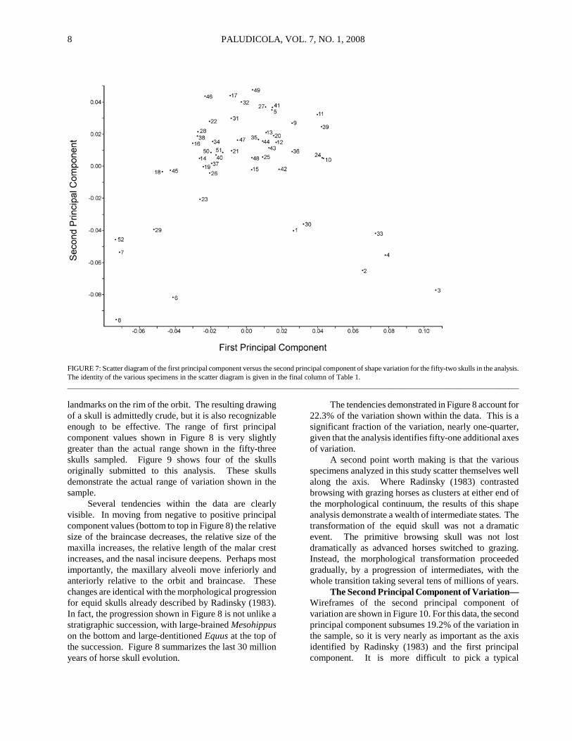
RESULTS A scatter plot of the first principal component versus the second principal component for the fifty-two skulls

submitted to this analysis is shown in Figure 7. If two specimens are closely adjacent on this plot, then their skulls have similar shapes. This is the first window produced by the principal components analysis of Morpholgika2. Movement of the cursor on this screen produces the wireframe depictions of skulls shown in subsequent figures. _____________________________________________

FIGURE 6. Transforming shape space into principal component coordinates. A typical shape equal to the centroid of all of the shapes in shape space is calculated, and a flat plane is fixed normal to the surface of the shape spheroid at the coordinates of this typical shape. The coordinates for each of the shapes in the analysis are then projected from the shape spheroid onto this flat planes on lines that are normal to the plane. ________________________________________________________ The First Principal Component of Variation—Shape changes along the first principal component of morphological variation are shown in Figure 8. I have chosen to display wireframe images, as they are easier to interpret than a scatter of landmarks. In this case, I used four lines to construct the wireframe: a line of points connecting peripheral landmarks that displays the outline of the specimen, a line of points connecting landmarks along the lower edge of the zygomatic arch, a line of points connecting landmarks along the upper edge of the zygomatic arch, and a line of points connecting the four


8

FIGURE 7: Scatter diagram of the first principal component versus the second principal component of shape variation for the fifty-two skulls in the analysis. The identity of the various specimens in the scatter diagram is given in the final column of Table 1. __________________________________________________________________________________________________________________________ landmarks on the rim of the orbit. The resulting drawing of a skull is admittedly crude, but it is also recognizable enough to be effective. The range of first principal component values shown in Figure 8 is very slightly greater than the actual range shown in the fifty-three skulls sampled. Figure 9 shows four of the skulls originally submitted to this analysis. These skulls demonstrate the actual range of variation shown in the sample. Several tendencies within the data are clearly visible. In moving from negative to positive principal component values (bottom to top in Figure 8) the relative size of the braincase decreases, the relative size of the maxilla increases, the relative length of the malar crest increases, and the nasal incisure deepens. Perhaps most importantly, the maxillary alveoli move inferiorly and anteriorly relative to the orbit and braincase. These changes are identical with the morphological progression for equid skulls already described by Radinsky (1983). In fact, the progression shown in Figure 8 is not unlike a stratigraphic succession, with large-brained Mesohippus on the bottom and large-dentitioned Equus at the top of the succession. Figure 8 summarizes the last 30 million years of horse skull evolution.

The tendencies demonstrated in Figure 8 account for 22.3% of the variation shown within the data. This is a significant fraction of the variation, nearly one-quarter, given that the analysis identifies fifty-one additional axes of variation. A second point worth making is that the various specimens analyzed in this study scatter themselves well along the axis. Where Radinsky (1983) contrasted browsing with grazing horses as clusters at either end of the morphological continuum, the results of this shape analysis demonstrate a wealth of intermediate states. The transformation of the equid skull was not a dramatic event. The primitive browsing skull was not lost dramatically as advanced horses switched to grazing. Instead, the morphological transformation proceeded gradually, by a progression of intermediates, with the whole transition taking several tens of millions of years. The Second Principal Component of Variation—Wireframes of the second principal component of variation are shown in Figure 10. For this data, the second principal component subsumes 19.2% of the variation in the sample, so it is very nearly as important as the axis identified by Radinsky (1983) and the first principal component. It is more difficult to pick a typical


9

morphocline out of the original data, because all of the original skulls are also overprinted with variation along the first principal component. But four skulls in the morphocline are shown in Figure 11. _____________________________________________

FIGURE 8. Wireframe drawings of the first principal component of variation. The range of variation shown is very slightly greater than the range shown by the actual sample. ________________________________________________________ Unfortunately, this second axis of variation is of difficult interpretation. The two outstanding tendencies in the data are expressed at opposite ends of the skull. At the back of the skull, the relative size of the braincase changes little on the second axis, but the orientation of the braincase changes significantly. For negative values of the second principal component (at the bottom of Figure 10), the facial angle between the sphenoids and the pterygoids is obtuse. As the second principal component increases, the facial angle becomes more acute. At the front of the skull, the nasals clearly move anteriorly as you move up the figure, and the depth of the nasal notch decreases. At the center of the skull, the orbit, the zygomatic arch, and the tooth row demonstrate relatively

FIGURE 9: Four of the drawings upon which this analysis is based chosen and arranged so as to demonstrate the morphocline along the first principal component of variation. ________________________________________________________ fixed relations across all values of the second principal component. Largely because the second principal component segregates all of the anchitheriines in the sample with high positive values, the second principal component may be separating browsers from grazers. Differences at the back of the skull in the facial angle accord well with this hypothesis. Browsers browse with the head flexed on an erect neck. Grazers graze with the head extended from a flexed neck. But I find no corroboration for the browsing-grazing hypothesis in the rostrum. Comparative studies of mammalian rostra suggest that a broad incisor arcade is the hallmark of a grazing dentition (Gordon and Illius, 1988; Janis and Ehrhardt, 1988), and associate retracted nasals with a proboscis (Radinsky, 1965).


10

Neither of those conclusions seems appropriate to the tendencies revealed in the present study. ____________________________________________

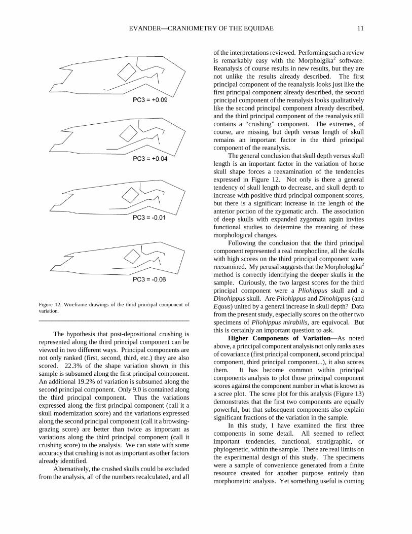
Figure 10: Wireframe drawings of the second principal component of variation. Again, the range of variation shown in this diagram is very slightly greater than the range shown by the actual sample. _________________________________________________________ I would hope that broader studies of ungulate rostra using the present technique might shed additional light on this area of the skull. It is not that the rostrum has received little attention from functional anatomists or systematists, but existing methodologies have produced a meager suite of generalizations. The present study suggests a significant morphocline in rostral morphology. We might understand more about why this morphocline is significant by studying this same area of the skull in deer or African antelope. The Third Principal Component of Variation—Wire frames of the shape changes along the third principal component of variation are shown in Figure 12. For negative values of the third principal component (at the bottom of Figure 12) the skulls are elongate from rostrum to occiput. For positive values of the third

principal component (at the top of Figure 12) the skulls are deeper inferior-superiorly from tooth row to frontals. This axis appears to represent some measure of post-depositional skull deformation. At least at one extreme, a perusal of the specimens themselves corroborates such a hypothesis. At the negative end of the scale, F:AM 111728 with PC3=-0.05, F:AM 69700 with PC3=-0.04, and UNSM 1353 with PC3=-0.04 all demonstrate collapse of the frontal suture on the top of the skull, suggesting vertical crushing. But collapse of the frontal suture is all too common in fossil horse skulls. F:AM 60810 with PC3=+0.06 (the largest value for the third principal component) also demonstrates collapse of the frontal suture. _____________________________________________

FIGURE 11. Four of the drawings upon which this analysis is based chosen and arranged so as to demonstrate the morphocline along the second principal component of variation.


11

Figure 12: Wireframe drawings of the third principal component of variation. ______________________________________________ The hypothesis that post-depositional crushing is represented along the third principal component can be viewed in two different ways. Principal components are not only ranked (first, second, third, etc.) they are also scored. 22.3% of the shape variation shown in this sample is subsumed along the first principal component. An additional 19.2% of variation is subsumed along the second principal component. Only 9.0 is contained along the third principal component. Thus the variations expressed along the first principal component (call it a skull modernization score) and the variations expressed along the second principal component (call it a browsing-grazing score) are better than twice as important as variations along the third principal component (call it crushing score) to the analysis. We can state with some accuracy that crushing is not as important as other factors already identified. Alternatively, the crushed skulls could be excluded from the analysis, all of the numbers recalculated, and all

of the interpretations reviewed. Performing such a review is remarkably easy with the Morpholgika2 software. Reanalysis of course results in new results, but they are not unlike the results already described. The first principal component of the reanalysis looks just like the first principal component already described, the second principal component of the reanalysis looks qualitatively like the second principal component already described, and the third principal component of the reanalysis still contains a “crushing” component. The extremes, of course, are missing, but depth versus length of skull remains an important factor in the third principal component of the reanalysis. The general conclusion that skull depth versus skull length is an important factor in the variation of horse skull shape forces a reexamination of the tendencies expressed in Figure 12. Not only is there a general tendency of skull length to decrease, and skull depth to increase with positive third principal component scores, but there is a significant increase in the length of the anterior portion of the zygomatic arch. The association of deep skulls with expanded zygomata again invites functional studies to determine the meaning of these morphological changes. Following the conclusion that the third principal component represented a real morphocline, all the skulls with high scores on the third principal component were reexamined. My perusal suggests that the Morphologika2 method is correctly identifying the deeper skulls in the sample. Curiously, the two largest scores for the third principal component were a Pliohippus skull and a Dinohippus skull. Are Pliohippus and Dinohippus (and Equus) united by a general increase in skull depth? Data from the present study, especially scores on the other two specimens of Pliohippus mirabilis, are equivocal. But this is certainly an important question to ask. Higher Components of Variation—As noted above, a principal component analysis not only ranks axes of covariance (first principal component, second principal component, third principal component...), it also scores them. It has become common within principal components analysis to plot those principal component scores against the component number in what is known as a scree plot. The scree plot for this analysis (Figure 13) demonstrates that the first two components are equally powerful, but that subsequent components also explain significant fractions of the variation in the sample. In this study, I have examined the first three components in some detail. All seemed to reflect important tendencies, functional, stratigraphic, or phylogenetic, within the sample. There are real limits on the experimental design of this study. The specimens were a sample of convenience generated from a finite resource created for another purpose entirely than morphometric analysis. Yet something useful is coming


12

FIGURE 13: Scree plot. The scree plot continues approaching the x axis as the diagram proceeds to the right, reflecting the diminishing importance of succeeding principal components. Only fifteen principal components are shown. _____________________________________________ from the results. I do not want to push the conclusions beyond the limits of the data. Better data, from more specimens and collected expressly for morphometric study, are available. The current study clearly calls for moving in the direction of better data.

CONCLUSIONS It seems that two important conclusions are possible as a result of this study. The first conclusion is that morphometric analysis of landmark data taken from fossil horse skulls reveals some important axes of covariation. One of these axes was previously identified by Radinsky (1983). At least two other axes of covariation are summarizing tendencies that invite additional study. Both of these additional axes seem to be summarizing tendencies that should be important functionally. All three of these higher axes might be of use phylogenetically. The second conclusion is that the Frick skull illustrations, because they were accomplished with a suspension pantograph and because they were drawn at a scale of 1:1, are amenable to morphometric analysis. These illustrations constitute a significant graphic database of mammalian variation for the late Tertiary. The prospectus for future study seems bright. The instrument exists for digitizing landmarks in three dimensions. Morphologika2 has the capability to analyze this three-dimensional input. The Frick Collection contains literally hundreds of skulls that might be digitized. The functional importance of the second and third components of the present investigation need to be studied. Additional data can only help in understanding these covariances.

ACKNOWLEDGEMENTS I wish to thank Jacob Mey, Rebecca Rudolph, and especially Angela Klause for access to the large-format scanner in the Microscope and Imaging Facility at the American Museum of Natural History. Chester Tarka knew significant details of the artistic techniques of the Frick artists, and communicated that knowledge to me. Without that seed, this paper would not have been possible. Lorraine Meeker provided honest assessment of the illustrations, sharing her talent generously. William Harcourt-Smith guided me to the PAST, tpsDig, and Morphologika2 software on the internet. He also has shared his talent generously. I would be remiss if I did not personally thank some of the authors who have shared their understanding of complex mathematical concepts by writing freely-available software for morphometricians. Øyvind Hammer, David A. T. Harper, and P. D. Ryan have written PAST, a general statistical package for paleontological applications. Although I do not explicitly cite it above, I relied upon their package frequently in the course of this study. F. James Rohlf coded tpsDig as just one of several morphometric packages available from the Stonybrook Morphometrics site. Six months ago I was determined to sit down and generate landmark data manually using the show info window and measure tool in Photoshop. Rohlf’s software saved me that labor, allowing a focus on the horses I study rather than the difficult process of transitioning from a Photoshop image to landmark coordinates. Paul O’Higgins and Nicholas Jones created Morphologika2, which serves as a bridge between a theory of landmarks and the reality of a morphometric analysis in shape space. All of these groups have hidden powerful mathematics and difficult computer coding in attractive, easy-to-use packages. These packages are elegant creations that deserve special thanks to their authors for sharing them so freely. Finally, I am honored that Richard Tedford, William Hartcourt-Smith, and Thomas Kelly volunteered to review this contribution. Their careful reading of the manuscript and lucid criticisms significantly improved the final result. I remain responsible for any remaining mistakes.

LITERATURE CITED Gordon, I. J. and A. W. Illius. 1988. Incisor arcade

structure and diet selection in ruminants. Functional Ecology 2:15-22.

Janis, C. M. and D. Ehrhardt. 1988. Correlation of relative muzzle width and relative incisor width with dietary preference in ungulates. Zoological Journal of the Linnean Society 92:267-284.


13

O’Higgins, P. and N. Jones. 1998. Facial growth in Cercocebus torquatus: an application of three-dimensional geometric mophometric techniques to the study of morphological variation. Journal of Anatomy 193:251-272.

O’Higgins, P. and N. Jones. 2006. Morphologika2, tools for shape analysis. Functional Morphology and Evolution Research Group, Hull York Medical College, University of York.

Radinsky, L. B. 1965. Evolution of the tapiroid skeleton from Heptodon to Tapirus. Bulletin of the Museum of Comparative Zoology 134:69-106.

Radinsky, L. B. 1983. Allomerty and reorganization in horse skull proportions. Science 221:1189-1191.

Rohlf, F. J. 2005. TpsDig, digitize landmarks and outlines, version 2.05. Department of Ecology and Evolution, State University of New York at Stony Brook.

craniometry of the equidae part i: two-dimensional … · 07.05.2018 · f:am 60823 pliohippus...

Documents