Credit Crunches, Asset Prices and Technological Change

Luis AraujoMichigan State University

Qingqing CaoMichigan State University

Raoul Minetti∗

Michigan State University

Pierluigi MurroLuiss University

Abstract

We investigate the effects of a credit crunch in an economy where firms can retain a maturetechnology or adopt a new technology. We show that firms’ collateral eases firms’ access to creditand investment but can also inhibit firms’ innovation. When this occurs, a contraction in theprice of collateral assets squeezes collateral-poor firms out of the credit market but fosters theinnovation of collateral-rich firms. The analysis reveals that the credit and asset market policiesadopted during recent credit market crises can boost investment but slow down innovation. Wefind that the predictions of the model are consistent with the innovation patterns of a largesample of European firms during the 2008-2010 credit crisis.

Keywords: Credit Crunch, Technological Change, Collateral.JEL Codes: E44; G21; G01.

∗Department of Economics, Michigan State University. E-mail: minetti@msu.edu. Phone: +1-517-355-7349.Address: 486 W. Circle Drive, 110 Marshall-Adams Hall, Michigan State University, East Lansing, MI 48824-1038.We wish to thank the editor and two anonymous referees for their comments. For comments and conversations, wealso wish to thank Giorgio Gobbi, Luigi Guiso, Maurizio Iacopetta, Matteo Iacoviello, Nobuhiro Kiyotaki, RowenaPecchenino, Susan Chun Zhu and seminar participants at Bank of France, Bank of Portugal, Boston College, EinaudiInstitute for Economics and Finance, Fed Board of Governors, London School of Economics (FMG/ESRC Conference),North Carolina State University, Stockholm School of Economics (Finance Department), University of Kentucky,University of Michigan Ross Business School (Finance Department), Chicago Fed “Summer Workshop on Money,Banking, Payments and Finance”, American Economic Association Meetings, Midwest Meetings in Economic Theoryand in Macroeconomics, SKEMA Workshop on “Credit Frictions and Money” (Nice), OFCE-Sciences Po Workshopon “Finance, Growth and Crises” (Paris). All remaining errors are ours.

Credit Crunches, Asset Prices and Technological Change

Abstract

We investigate the effects of a credit crunch in an economy where firms can retaina mature technology or adopt a new technology. We show that firms’ collateral easesfirms’ access to credit and investment but can also inhibit firms’ innovation. When thisoccurs, a contraction in the price of collateral assets squeezes collateral-poor firms outof the credit market but fosters the innovation of collateral-rich firms. The analysisreveals that the credit and asset market policies adopted during recent credit marketcrises can boost investment but slow down innovation. We find that the predictions ofthe model are consistent with the innovation patterns of a large sample of Europeanfirms during the 2008-2010 credit crisis.

Keywords: Credit Crunch, Technological Change, Collateral.JEL Codes: E44; G21; G01.

1 Introduction

During the financial crisis that started in 2008, a major drop in the value of collateral assets,especially real estate, triggered a credit contraction, prompting firms to reduce their investments.The literature offers well-established arguments for interpreting these effects of a credit crunch.When entrepreneurs cannot commit to repay lenders, collateral eases their access to credit.1 Thus,aggregate shocks that erode collateral asset values depress total investment by hindering firms’access to external finance (Kiyotaki and Moore, 1997; Lorenzoni, 2008; Holmstrom and Tirole,1997; Den Haan, Ramey and Watson, 2003; Buera and Moll, 2015).

While useful to explain key transmission mechanisms of a credit market crisis, these argumentsonly yield partial insights into the effects of a credit crunch on technological change. Financialcrises appear to have contrasting effects on technological change. The OECD (2009) reviews severalpieces of evidence and concludes that credit market crises can certainly damage innovative firmsbut also be “times of industrial renewal”. Field (2011) documents that the Great Depression wasa period of major innovations for the U.S. economy.2 These innovations ranged from Teflon inpetrochemicals industries to household appliances, such as the radio and refrigerator, and formedthe basis for the post-World War II economic expansion. In South Korea and in Finland, thenumber of innovative firms boomed during and in the immediate aftermath of the 1990s financialcrises (OECD, 2009). And firm-level surveys reveal that while the credit crisis that started in 2008depressed the innovation efforts of firms with difficult access to credit, such as young businesses withscarce collateralizable wealth, it also stimulated the innovation activity of other firms, especiallymore established businesses with more pledgeable assets and easier access to credit (see, e.g.,Hall, 2011; European Commission, 2012; Voigt and Moncada-Paterno-Castello, 2009; Cincera,

1Ex post, after entrepreneurs default, lenders can repossess collateral and this compensates for the limited pledge-ability of entrepreneurs’ output; ex ante, lenders’ threat to repossess collateral deters entrepreneurs’ misbehavior.

2Further back in history, the Long Depression started in 1873 was marked by the introduction of major innovations.

1

Cozza, Tubke and Voigt, 2012, and references therein). In Section 2, we will uncover evidence insupport of these conclusions by exploring survey data on the innovation activity of about 15,000European firms during the 2008-2009 credit crisis. The results will suggest that, while the majorityof firms responded to the 2008-2009 credit crunch and drop in collateral asset prices by postponinginnovation, a non-negligible number of firms responded to shrinking credit and collateral valuesby investing in innovation. Such firms were concentrated in the segment of businesses with largepledgeable assets, whereas firms with little collateral assets scaled down their innovation activity.

These observations elicit fundamental questions: Can we build a model economy that capturesthese contrasting effects of credit market crises on innovation? In such an economy, under whatconditions does a credit crunch triggered by a drop in collateral values depress or stimulate inno-vation? And what policies are more innovation-friendly during a credit crunch? This paper takes astep towards addressing these questions. Building on the above observations, we focus on the inno-vation propensity within incumbent businesses that rely on collateral-based funding. We posit aneconomy where entrepreneurs operate a mature technology or innovate and adopt a new technology.Lenders, in turn, acquire information that is essential for repossessing and liquidating productiveassets pledged as collateral when entrepreneurs default (as in Diamond and Rajan, 2001, for exam-ple). Lenders’ information on collateral assets eases entrepreneurs’ access to credit but can makelenders reluctant to finance entrepreneurs’ innovation. In fact, the assets of the new technology aremore illiquid and firm specific and, hence, less pledgeable as collateral than the assets of the maturetechnology. Furthermore, lenders’ information on the assets of the mature technology is (partially)specific and non-transferable to the assets of the new technology. Therefore, expecting that the in-formation they have accumulated on mature collateral assets will go wasted if entrepreneurs switchto the new technology, lenders may hinder entrepreneurs’ innovation efforts.

The distribution of firms across collateral values replicates salient features of that obtainedin previous general equilibrium models of the credit market (e.g., Holmstrom and Tirole, 1997).Collateral-poor firms lack access to credit because they cannot pledge enough expected returns tolenders. Firms with medium and rich collateral assets, instead, obtain credit. The novelty consistsof firms’ technology adoption. When lenders’ technological inertia arises, while firms with a mediumvalue of collateral potentially innovate, collateral-rich firms retain the mature technology. In fact,their lenders expect a large depreciation in the value of their information if the mature technologyis abandoned in favor of the new technology.

We study the effects of a contraction in the price of collateral assets (e.g., as in Holmstromand Tirole, 1997, and Kiyotaki and Moore, 1997). Following a drop in the asset price, marginalfirms with collateral assets just sufficient to obtain credit are squeezed out of the credit marketbecause they can no longer pledge enough expected returns to lenders. This tends to reduce totalinvestment and innovation. Consider next collateral-rich firms. The asset price drop erodes thevalue of the information acquired by their lenders on mature collateral assets, mitigating lenders’potential technological inertia. This can foster the innovation of collateral-rich firms. Overall, whilethe asset price drop depresses total investment, its impact on innovation depends on the relativemagnitudes of the drop in the innovation of firms squeezed out of the credit market and the increasein the innovation of collateral-rich firms.3

The analysis delivers novel policy implications. We investigate the effects of two unconventionalpolicies implemented by central banks and governments during the recent credit crisis: an interven-tion in the collateral asset market aimed at bolstering the asset price and a policy of direct lending

3In the paper, we characterize conditions under which an asset price drop is more likely to trigger an increase ininnovation. For example, we relate the likelihood of this scenario to the verifiability of the output of projects and tothe probability of project success.

2

to collateral-poor firms. We find that both policies boost total investment but may dampen theincrease in the innovation of collateral-rich firms after the shock. Notably, the asset market policyturns out to be more taxing for innovators than the direct lending policy.

In the last part of the paper, we revisit the mechanisms of the model under richer structuresof the credit sector and the corporate sector. The goal is to assess under what structures of thecredit and corporate sectors a credit crunch is more likely to depress or stimulate innovation. Inthe credit sector, we allow for information-intensive credit relationships between firms and lendersin which lenders obtain more information on firms’ collateral assets (Diamond and Rajan, 2001).We find that, following a contraction in the price of collateral assets, the increase in the innovationof collateral-rich firms can entail a reduction in the number of credit relationships. In turn, thiscan dampen the stimulus to output triggered by innovation. In the corporate sector, we allow formanagerial firms and managers’ technological inertia due to higher riskiness of the new technology.We then investigate how managers’ inertia interacts with lenders’ potential technological inertia.

This paper especially relates to two strands of literature. The first strand investigates theimpact of a disruption in the financial structure on aggregate investment (e.g., Gertler and Karadi,2011; Gertler and Kiyotaki, 2010, 2015). In this literature, we borrow some properties of ourmodelling strategy, such as the focus on a finite horizon economy, from Holmstrom and Tirole(1997). Other related papers in this literature include Den Haan, Ramey and Watson (2003),Dell’Ariccia and Garibaldi (2001), Buera and Moll (2015) and Catherine, Chaney, Huang, Sraerand Thesmar (2017). Buera and Moll (2015) study the effects of a tightening of collateral constraintson investment wedges in a model with credit frictions and heterogeneous firms. Catherine et al.(2017) structurally estimate the impact on investment and output of collateral shocks in a modelwith heterogeneous firms.4 While in these studies a credit tightening depresses investment, in oureconomy it depresses investment but may foster technological change.

The second related strand of literature analyzes the impact of recessions on firms’ innovationthrough the credit market (e.g., Caballero and Hammour, 2005; Ramey, 2004; Garcia-Macia, 2017;Wang, 2017). Caballero and Hammour (2005) show that, because of credit frictions, productionunits can be destroyed at an excessive rate during a recession and the subsequent recovery canoccur more through a slowdown in the destruction rate than through an increase in the creationrate. Ramey (2004) shows that if financial managers have empire-building incentives, during down-turns they can discard efficient projects to preserve the size of their portfolios. This paper putsforward a view opposite to these studies: while it depresses investment, a credit tightening canmitigate lenders’ technological inertia. In this regard, our analysis shares some features with theShumpeterian view of recessions as moments of creative destruction. For example, in Caballeroand Hammour (1994) during recessions innovative production units can more easily enter and dis-place outdated ones. However, we do not focus on the innovations of newly formed start-ups, butrather on changes in the innovation propensity within incumbent businesses, showing how changesin the value of their collateral assets can alter the incentives of their lenders to support innovation.Accordingly, we focus on collateralized lending by financial institutions, rather than early-stageprivate equity or growth funding. Recent studies in this literature focus increasingly on the designof effective policies for promoting innovation. Garcia-Macia (2017) investigates an economy whereheterogeneous firms invest in physical and intangible capital. Intangible capital is harder to seize bycreditors and hence incurs into higher financing costs. In a financial crisis, these costs rise and theresulting fall in intangible investment amplifies the crisis. Garcia-Macia (2017) finds that a policyof transfers conditional on firm age may speed up the recovery from a crisis more than credit sub-

4Gilchrist, Sim and Zakraj (2014) quantify the output loss due to misallocation of credit across firms. See alsoShourideh and Zetlin-Jones (2017).

3

sidies. Wang (2017) studies R&D investment and knowledge capital accumulation in an economywith credit frictions. Unlike physical capital, knowledge capital cannot be pledged as collateral.Wang (2017) shows that firms with initially high knowledge capital engage in precautionary savingsto raise their collateralizable financial assets. He also examines the impact of industrial policies,finding that tax credits for R&D investment can boost output more than policies that encouragethe use of intellectual property as collateral.

The remainder of the paper unfolds as follows. In Section 2, we provide background evidencefor key mechanisms of the model. In Section 3, we present the baseline model. Section 4 solves forthe equilibrium. In Section 5, we conduct experiments aimed at mimicking a credit market crisis.Section 6 considers policies. Section 7 studies extensions while Section 8 concludes. Appendix Acontains additional details on the data and the empirical analysis while Appendix B contains themain proofs (baseline model, Sections 3-5). Further details of the derivations and additional resultsare relegated to the online Supplement.

2 Empirical Background

As noted, various pieces of evidence point to a possible role of credit market crises in stimulatingthe start of innovative plans by established firms with large pledgeable collateral, while depressingthe access to credit and the innovative plans of collateral-poor firms. To gain further intuition,in this section we exploit information from a large survey of European firms conducted in 2010with reference to the years 2007-2009. Our data source is the EU-EFIGE data set, collected aspart of the EFIGE project (European Firms in a Global Economy: internal policies for externalcompetitiveness) supported by the Directorate General Research of the European Commissionand coordinated by the Bruegel Institute. The survey targets a representative sample at thecountry level of almost 15,000 manufacturing firms with more than 10 employees in seven Europeancountries (Austria, France, Germany, Hungary, Italy, Spain, United Kingdom). The data setincludes quantitative and qualitative information on firms’ R&D, innovation, labor organization,financing and organizational activities. Questions related to the behavior of firms during the 2008-2010 financial crisis were also included in the survey. We complement the EFIGE data set withfirms’ balance-sheet information from the BvD-Amadeus database.

The EFIGE data set is ideally suited for our purposes. First, it surveys firms in European coun-tries generally characterized by a strong importance of banking sectors in firm financing. Second,it covers the period of the credit market crisis that started in 2008. The seven countries covered bythe EFIGE survey experienced a sizeable credit crunch from 2008 to 2009, with the average creditto non-financial businesses dropping by about 1.2% in real terms from the last quarter of 2008 tothe last quarter of 2009 (source: BIS, Credit to the Non-Financial Sector, section on non-financialfirms). Third, one of the main goals of the survey was to investigate firms’ response to deteriorat-ing credit market conditions from 2008 to 2009. Thus, the survey questionnaire explicitly askedthe firms whether from 2008 to 2009 they increased or decreased their activities on a number ofrelevant margins. Importantly for our purposes, firms’ innovation activity is one of the marginsinvestigated by the survey. Using the survey questions on innovation, we construct a dummy vari-able that takes the value of one if the firm declares that in 2008-2009 it engaged in innovations thatresulted in products and product features that were innovative with respect to products existingin the market. We label this indicator variable “engagement in innovations in 2008-2009”. Wealso construct an alternative variable using a somewhat stricter definition: a dummy variable thattakes the value of one if the dummy “engagement in innovations in 2008-2009” takes the value ofone and in addition the firm declares that in 2008-2009 it did not postpone innovation plans and

4

that it actually expanded its range of products (signalling non-marginal innovations). We labelthis second indicator variable “start or acceleration of non-marginal innovations in 2008-2009”. Inaddition, our data provide rich information on the availability of collateralizable assets as well asdetails on banks’ lending technologies, including banks’ emphasis on firms’ collateral when grantingcredit (see Appendix A for more details on the variables).

Before turning to the empirical analysis, it is useful to check the relevance of external financingfor firms’ innovation activities. The survey asks the firms the percentage of funding for investmentsthat comes from internal funds, intragroup financing, venture capital, bank credit, public funding,leasing and factoring, or other. It also asks the firms whether the composition of funding forinnovation activities and R&D is the same as for investments broadly meant. In line with figuresfrom the literature (e.g., Allen and Gale, 2001), the firms declare that the percentage of bankfunding for investments approximately equals 26.5%, versus slightly more than 50% of internalfinancing. Around two thirds of the firms declare that the share of bank funding for innovationactivities and R&D is the same as for other investments. When we consider firms with below themedian size (employees) the share of bank funding for investments approximately equals 30% (witharound two thirds declaring the same relevance for innovation and R&D funding). These figuresindicate that a substantial share of funding for innovation activities does not come from internalfinancing and, in particular, that bank credit is an important source of funding for such activities.

In Table 1, we use the information provided by the EFIGE data set in two ways. In Panel A,we explore whether during the credit market crisis (2008-2009) there were significant differencesbetween firms that invested in innovation and firms that instead postponed their innovation plans.Unsurprisingly, the panel reveals that during the credit crunch about 85% of the firms postponedinnovation plans. Yet, about 15% of the firms in the sample declare that during the credit crunchthey instead started or accelerated non-marginal innovation plans. Importantly for our purposes,the panel shows that such firms were of similar size and age as the firms that postponed innovationbut exhibited a significantly larger availability of collateralizable assets, especially fixed assets easilypledgeable as collateral. Panel A further suggests that during the crisis banks’ emphasis on collateraltended to be associated with a drop in the innovation activity of firms with little pledgeable assetsbut with some increase in the propensity to innovate of firms with large pledgeable assets. Finally,the panel indicates stronger importance of credit relationships for innovative firms than for firmsthat postponed innovation.

While the 2008-2009 credit crunch was pervasive, some firms suffered from its effects more thanothers. Further, our theoretical analysis stresses the impact of a drop in the value of collateralizableassets. In Panel B of Table 1, we then dig deeper into the data and test whether the firms thatduring the 2008-2009 credit crunch experienced a contraction in the value of their fixed, pledgeableassets exhibited a tendency to invest in innovation or to postpone innovation plans. Again, ourmain interest is whether firms with larger initial collateral responded differently to a drop in thevalue of their pledgeable fixed assets, investing in innovation rather than postponing innovation(see the interaction term in the regressions). We saturate all the probit regressions in Panel B witha full set of country and two-digit industry dummies and in columns 5-8 we further include variousfirm-level controls, such as proxies for firm size, age and labor productivity (the inclusion of thesecontrols entails a loss of observations). The results in the panel reveal that during the crisis thefirms with little assets that experienced a contraction in the value of fixed assets did not engage ininnovations and indeed postponed innovation plans following such a contraction. By contrast, thefirms with initially large assets responded to a contraction in the value of fixed assets by engagingin innovations and actually starting or accelerating non-marginal innovation plans. For example,in column 1 the estimated coefficient on the change in the value of fixed assets is positive and

5

Tab

le1:

Eu

rop

ean

Fir

ms’

Inn

ovat

ion

du

rin

gth

e20

08-2

009

Cre

dit

Mar

ket

Cri

sis

6

equal to 0.064 while the interaction term with the dummy for larger-than-median assets is negativeand equal to -0.112. In column 2, the estimated coefficient on the change in fixed assets is againpositive (equalling 0.061) while the coefficients on the interaction terms with the dummies for the3rd and 4th asset quartiles are significantly negative (and equal to -0.095 and -0.124, respectively).These findings are confirmed when we reestimate the regressions for different subsamples based onfirms’ initial asset value, rather than inserting interaction terms (see, e.g., columns 3-4 and 13-14).Further, in columns 9-10 we reestimate the regression in column 1 separately for firms that declarethat their banks are significantly involved in the financing of the firm’s investments and for firms forwhich banks have little involvement. We find that, for firms with initially large assets, the tendencyto innovate in response to a drop in fixed assets manifested itself especially when their banks wheresignificantly involved in investment financing (compare the interaction terms in columns 9 and 10).

Consistent with the evidence mentioned in Section 1 and with the conclusions of OECD (2009),the results in Table 1 thus suggest that during the 2008-2009 European credit crisis, while themajority of firms responded to the contraction in credit and collateral values by scaling down theirinnovation plans, a non-negligible share of firms responded by investing in innovation. Such firmswere concentrated in the segment of businesses with relatively large availability of assets pledgeableas collateral.

2.1 Robustness

We conduct several tests to verify the robustness of the findings in Table 1. To conserve space, wepresent the robustness tests in the Appendix Tables A.1-A.2. The reader could wonder whetherfirms with large availability of collateralizable assets have also a large stock of outstanding debt. Ifthat were the case, the size of total assets or fixed assets of a firm might not reflect accurately theavailability of assets pledgeable to financiers. In a first set of robustness tests we then experimentby adding the firm’s leverage as a control (where leverage is total liabilities over total assets). Theresults remain virtually unaffected and leverage appears to have no (or at most limited) power inexplaining firms’ innovation decisions (Table A.1, columns 1-5). To further control for outstandingdebt obligations that could reduce collateral asset availability, in columns 6 and 7 of Table A.1 wealso insert the ratio of bank debt over the total liabilities of the firm and the ratio of short-termbank debt over total liabilities. Bank debt is generally collateralized while corporate bonds are not;moreover, short-term debt often entails more stringent debt obligations than long-term debt. Theresults are robust to including these further controls for firms’ debt obligations.5

The reader might also wonder whether in the baseline regressions of Table 1 the effect of assetson innovation reflects the availability of internal cash. In columns 8-17 of Table A.1, we include twoproxies of cash availability: the firm’s cash flow in 2008 (columns 8-12) and the firm’s liquidity ratio,defined as the stock of cash and cash equivalents over total assets in 2008 (columns 13-17). Theresults remain essentially unaltered and the proxies for cash availability are generally insignificant.

Firms’ innovation decisions can be dictated by expectations about the net profit of the business.While we cannot directly observe such expectations, in Table A.2, Panel C, we include a measureof the firm’s profitability in the years of the sample, the firm’s return on assets (ROA). The resultsremain virtually unchanged whether we control for the firm’s ROA in 2008 (columns 7-11) or theaverage ROA over 2008 and 2009 (not tabulated). And columns 12-13 show that the results remainunchanged after controlling for an additional proxy of firm labor productivity, the number of skilledblue collar workers of the firm.6

5Supplementary Table S.3 also contains the estimates obtained after controlling for banks’ emphasis on collateral.6In untabulated tests, we also experimented with other proxies for the human capital of the firm.

7

A possible further concern could be that there is some reverse causality from innovation tocollateral asset availability. In our context, we do not expect the start or acceleration of innovationplans during the crisis period to directly influence the stock of collateral with which a firm entersthe period. However, to further assuage lingering doubts, we experiment by using a measure ofcollateral availability which is driven by the inherent technological characteristics of the firm’sindustry. In particular, we employ the sectorial measure of asset tangibility constructed by Braun(2005). In Panel A of Table A.2, columns 1-2, we then reestimate the regressions by inserting thismeasure of asset tangibility interacted with the change in the firm’s fixed assets. The results areconsistent with those obtained in Table 1 using total assets: for firms with higher asset tangibility,a contraction in fixed assets promotes innovation.7

In Panel B of Table A.2, columns 3-6, we experiment with an alternative definition of thedependent variable. To further narrow down the firms that started or accelerated innovation plansduring 2008-2009, we code a dummy that equals one if the indicator variable “start or accelerationof non-marginal innovations” takes the value of one and, on top of this, the firm applied for a patentin 2008-2009 or purchased foreign R&D and engineering services. Using this definition yields almostidentical insights.

Finally, the reader might wonder whether during the crisis firms with limited collateral andtight financial and profitability conditions engaged in a “gamble for resurrection behavior” byundertaking risky but potentially profitable innovations. If that were the case, some of thesefirms could have failed during the crisis, exiting the sample. While we lack information on suchpotential sample dropouts, we can carry out two tests that provide some evidence regarding thepresence of a gambling for resurrection behavior in our sample. In columns 14-18 of Table A.2,employing a propensity score matching model, we test whether indeed the impact of the treatment(collateral availability) on innovation decisions does not reflect riskiness, profitability, or defaultprobability of the firm. In particular, we estimate the determinants of innovation in a sample ofmatched firms above and below the median total asset value and that feature similar profiles ofriskiness (Z-score),8 profitability, age, industry, and country. Matched firms were selected in twoalternative ways: (i) without replacement using all matching firms within the predefined propensityscore distance (caliper) δ = 0.001 and (ii) using the control firm with the closest propensity score(nearest neighbor), without resampling or distance restrictions. With both methods, the resultsobtained in this matched sample appear to be virtually identical to those in the full sample.9

A second way in which we can detect the presence of “gambling for resurrection” is to verifywhether firms in our sample on the verge of distress at the onset of the crisis and that choseto innovate during the crisis exhibited higher propensity to fail in the following years. Matchinginformation on firm exit from the Orbis and Amadeus databases to the firms in our sample, wethen constructed a proxy for firm exit taking the value of one if the firm exited in 2010 or 2011(“exit by 2011”); we also constructed an indicators for exit in 2010-2012 (“exit by 2012”). Next,we verified to what extent these proxies for exit correlate with innovation activities for firms withsigns of distress at the onset of the crisis (firms with total assets below the median, firms withROA below the median and, in line with Altman et al., 1977, firms with a Z-score below a cutoff(1.8) which is reputed to be a sign of incipient distress). Supplementary Table S.4 gathers a widerange of correlations. We find no evidence that firms on the verge of distress at the onset of thecrisis exhibited a positive correlation between innovation and propensity to exit in 2010, 2011 and

7As an alternative check, we also considered the measure of asset redeployability in Kim and Kung (2017), obtainingsimilar results.

8The Z-score for non-listed firms is constructed as in Altman et al. (1977) and following studies.9In columns 14-18 we display the estimates obtained with the first method.

8

2012 (if anything, we find negative, though not significant, correlations between innovation and ourproxy for exit). These conclusions hold up when we regress the indicator for exit on innovationand on sector and country fixed effects. And similar insights are obtained if we replace the proxyfor exit with an indicator of distress after the crisis, the firm’s solvency ratio. Thus, it does notappear that distressed firms that innovated during the crisis had a higher propensity to fail in thefollowing years.

3 The Baseline Model

This section describes a general equilibrium model of the credit market where firms exhibit het-erogenous availability of collateralizable assets. Firms can retain a mature technology or potentiallyadopt a new technology. We then explore the impact on firms’ innovation of shocks to collateralasset values and the implications of policy interventions. Figure 1 illustrates the timing of eventswhile Table 2 summarizes the notation of the model.

3.1 Agents, goods, and technology

Consider a three-date economy (t = 1, 2, 3) populated by a unit continuum of entrepreneurial firmsand a continuum of investors of measure larger than one. There is a final consumption good, whichcan be produced and stored, and productive assets of two vintages, mature and new. Entrepreneurshave no endowment while each investor is initially endowed with an amount ω of final good. Allagents are risk neutral and consume on date 3.

Each entrepreneur can carry out one indivisible project that requires an investment i < ω offinal good. On date 1, an entrepreneur can choose an innovative plan for his project that cangenerate an innovation opportunity on date 2. If the innovative plan is chosen and the innovationopportunity arises, the entrepreneur adopts a new technology. Otherwise, the entrepreneur has toretain a mature, less productive technology. Under the mature (new) technology, on date 3 theentrepreneur transforms an amount i of final good into one unit of mature (new) assets. Withprobability π the project succeeds and the mature (new) assets yield an output y (y(1 +n)) of finalgood; otherwise the project fails and the entrepreneur goes out of business.

In case of failure, a fraction µa of assets can be recovered and redeployed outside the firm. acaptures the amount of collateralizable assets of an entrepreneur and is uniformly distributed acrossentrepreneurs over the domain [0, 1]. µ reflects the effort the entrepreneur exerts for the maintenanceof the collateralizable assets. This maintenance can be thought as acquiring information on thecollateral assets and their market or also as restraining from looting and asset depreciation.10 Wespecify a simple technology for the maintenance of collateral assets: an entrepreneur sustains a

per-unit effort cost of ζµ2

2 for achieving a level µ of maintenance.On date 3, each entrepreneur still in business can reuse one unit of liquidated assets, obtaining

an amount ηy of final good. y is an idiosyncratic output with a positive mass on zero. Theexpected value of y is θ, which is uniformly distributed across entrepreneurs over the domain [0, θ];η represents the aggregate productivity of liquidated assets.11

10Different classes of models focus on various activities of collateral asset maintenance and preservation and wedo not restrict attention to one particular interpretation. A broad empirical literature shows that borrowers’ actionscan significantly impair or enhance the actual liquidation value of collateral (see, e.g., Calomiris, Larrain, Liberti andSturgess, 2017, Udell, 2004, ILO, 2001, and references therein). In macroeconomic settings, firms are often assumedto engage in activities of capital repair (see, e.g., Gertler and Karadi, 2011).

11The heterogeneity in entrepreneurs’ ability to reuse assets generates a downward sloping asset demand.

9

Figure 1: Decisions of entrepreneurs and lenders. The bottom of the tree shows the repayments tothe lender in the event of project success.

3.2 Credit sector

Each entrepreneur can enter a credit contract with one investor on date 1. Following an establishedliterature, we allow the lender to exert some control over the entrepreneur’s production opportu-nities (see, e.g., Aghion and Bolton, 1992; Rajan, 1992). Precisely, consider the case in which theentrepreneur has chosen an innovative plan for his project. On date 2, the lender can carry outa costless action that affects the probability of the innovation opportunity: if she carries out thisaction, the opportunity will arise with probability 1−σA; otherwise, the opportunity will arise witha lower probability 1− σA (where 0 < σA < σA < 1).

The lender also acquires information on assets as a by-product of her financing activity. As inDiamond and Rajan (2001) and Habib and Jonsen (1999), this enables her (unlike other agents) toobtain value from the liquidation of the entrepreneur’s assets. Precisely, the liquidation value thelender recovers in the event of project failure and liquidation of the mature technology is pµa, wherep denotes the asset price; the rest is lost in the form of transaction costs.12 To capture the idea thatthe lender has instead lower ability to acquire experience about the assets of a new technology, weassume that the lender recovers less value from new assets than from mature assets (we normalizeto zero what she obtains in case of liquidation of the new technology).13

3.3 Contractual structure

As in Aghion and Bolton (1992) and Diamond and Rajan (2001), a lender cannot contractuallycommit to carry out her action that facilitates (increases the probability of) the innovation oppor-tunity because the action is non-verifiable; similarly, the level of collateral maintenance performed

12Throughout, unless otherwise stated, we let transaction costs be transfers rather than a real resource loss. Thisis without loss of generality.

13As discussed in Section 7.3, and shown in the Supplement, the results carry through with alternative specifications.In the Supplement, we consider an alternative case in which the lender has control over the success probability ofprojects (Section C.1 of the Supplement) and a case in which the lender has partial ability to liquidate the assetsof the new technology (Section B.3). We also study alternative settings where the new technology has a higher or alower success probability than the mature technology (Sections B.1 and B.2).

10

Table 2: Notation of the Model

Probability of project success π

Output of mature technology y

Productivity edge of new technology n

Collateral assets of firm a

Investment outlay of project i

Share of verifiable output l

Probability of innovation opportunity if lender facilitates 1− σA

Probability of innovation opportunity if lender hinders 1− σA

Aggregate productivity liquidated assets η

Idiosyncratic productivity liquidated assets θ

Lender’s bargaining power in renegotiation λ

Maintenance cost of collaterals ζ

Lender’s endowment ω

Note: The table describes the parameters and exogenous variables of the model.

by an entrepreneur is not verifiable in courts, implying that no contract can be written upon it. Im-perfect enforceability also limits agents’ commitment to pecuniary transfers and, hence, the designof pecuniary incentives for the lender. Specifically, in the event of project success, only a fractionl of the output is verifiable while the rest accrues privately to the entrepreneur. In the event ofproject failure and asset liquidation, the lender cannot commit the specific liquidation skills tiedto her information about the assets. Thus, as in Diamond and Rajan (2001), she can threaten towithhold her skills during the liquidation, forcing a renegotiation of the allocation of the liquidationproceeds. We denote by λ the bargaining power of the lender in the renegotiation.

Given this contractual structure, on date 1 the contract between a lender and an entrepreneurspecifies a loan amount of i and the repayment to the lender in the event of project success, con-tingent on the technology adopted. Precisely, if the entrepreneur does not choose an innovativeplan, the contract specifies the repayment rIm if the mature technology is successfully operated; ifthe entrepreneur chooses an innovative plan, the contract specifies the repayment rIm(rIn), if themature (new) technology is successfully operated. Since on date 1 there is perfect competitionamong investors, the contract maximizes the entrepreneur’s expected return subject to the en-trepreneur’s limited liability constraints rIm, r

Im ≤ ly, rIn ≤ l(1 + n)y, and the relevant constraints

of the lender.1415 These include the lender’s participation constraint and the lender’s incentiveconstraint if the entrepreneur wants to incentivize the lender to carry out the action that facilitatesinnovation.

3.4 Discussion

In the real sector, the difference between the two technologies is that the new technology producesmore output (y(1 + n) > y) but its assets have lower liquidation value (µnpa < µpa, where for

14Since assets purchased in the liquidation market have zero output with positive probability, an entrepreneur isunable to commit such liquidation output to a lender, on top of the output of his project. This feature captures in areduced form the difficulty to contractually pledge output from distant and unrelated activities.

15We do not impose a limited liability constraint for the lender. Implicitly, we are assuming that the lender hasmore than enough funds to make transfers to the entrepreneur on date 3, if needed. Adding a limited liabilityconstraint would not alter the results.

11

simplicity we have set µn = 0).16 The assets that embody new technologies and R&D results arelikely to be firm specific and illiquid, thus having little collateral value (Carpenter and Petersen,2002; Hall and Khan, 2003; Berlin and Butler, 2002; Rajan and Zingales, 2001; Garcia-Macia, 2017;Wang, 2017). Moreover, lenders typically have less experience in liquidating new vintages of assetsthan mature ones.

In the credit sector, two features are worth discussion: the control exerted by a lender and thecharacterization of information as asset liquidation skills. We share with Aghion and Bolton (1992),Rajan (1992), and Bhattacharya and Chiesa (1995), for example, the assumption that a lendercarries out an interim action that affects production opportunities. This action has several realworld counterparts. In an R&D race, it can consist of concealing the findings of the entrepreneur’sinternal research from his competitors (Bhattacharya and Chiesa, 1995); it can consist of providingthe entrepreneur with advice or information for expanding the firm’s technological frontier; if thelender has representatives on the board of the firm, as in the case of German and Japanese banks,it can consist of voting for an innovative strategy. In other circumstances, it can consist of arefinancing (Rajan, 1992): the need for refinancing is likely for a new technology which generallyyields little interim cash flow, especially at the R&D stage (Goodakre and Tonks, 1995). Aghion andBolton (1992) discuss examples of other actions of lenders which can affect innovation opportunities,such as supporting firms’ mergers and spin-offs.

We borrow the characterization of information as asset liquidation skills from Diamond andRajan (2001) and Habib and Johnsen (1999). The critical feature is that the lender acquires moreinformation than the entrepreneur and the other investors. As for the latter, following Diamond andRajan (2001), our assumption reflects the idea that the lender gathers more information on assetsthrough her financing activity. As for the former, “Because he [the entrepreneur] is a specialist atmaximizing the value of the asset in its primary use [...] it is reasonable to assume that he lacksthe skill even to identify the asset’s next best use or to recognize clearly the occurrence of the badstates” (Habib and Johnsen, 1999, p. 145).

4 Equilibrium

We solve the model in steps. First, we take the asset price as given and study the problems oflenders and entrepreneurs. We solve for the date-2 choice of collateral asset maintenance by anentrepreneur. We then solve for a lender’s choice α ∈ {A,A} between action (A) and inaction (A)on date 2, and her choice whether to finance an entrepreneur. We next solve for the date 1 choiceof an entrepreneur whether to engage in an innovative plan and her choice of contract.

4.1 Entrepreneurs’ collateral maintenance

When choosing the level of maintenance of the collateral assets, an entrepreneur maximizes

E(µ)− ζµ2

2pa

where E(µ) denotes the return that the entrepreneur expects to appropriate in case of liquidationof the mature assets. Lemma 1 characterizes the decision of collateral maintenance. The lemmashows that the maintenance effort increases as the probability of operating the mature technologyincreases (and therefore the probability of innovation declines).

16µ is an endogenous choice by entrepreneurs. It is positive in equilibrium, as the next section shows. In theSupplement (Section B.3), we consider a case in which new assets have positive liquidation value, though lower thanthat of mature assets. The results carry through.

12

Lemma 1 (Collateral maintenance). (i) If an entrepreneur adopts an innovative plan (I), andthe lender takes the action that facilitates innovation (A), the collateral maintenance effort is

µIA =(1− π)(1− λ)σA

ζ.

(ii) If an entrepreneur adopts an innovative plan (I), while the lender chooses inaction (A), themaintenance effort is

µIA =(1− π)(1− λ)σA

ζ.

(iii) If an entrepreneur does not adopt an innovative plan (I), the maintenance effort is

µI =(1− π)(1− λ)

ζ.

As σA < σA < 1, µIA < µIA < µI .

4.2 Lenders

Let us consider the case in which an entrepreneur chooses an innovative plan on date 1 and let usstudy the date 2 decision of his lender whether to carry out the action that facilitates innovation.The lender compares her expected return if she facilitates innovation with her expected return ifshe hinders it. Assuming that she breaks a tie in favour of innovation, she will carry out the actionif and only if

(1− σA)πrIn + σA[πrIm + λ(1− π)µIApa

]≥ (1− σA)πrIn + σA

[πrIm + λ(1− π)µIApa

].

Using the solution of µIA and µIA, the above inequality can be rewritten as

rIn − rIm ≥(σA + σA)(1− π)2λ(1− λ)pa

πζ. (1)

Inequality (1) is the lender’s incentive constraint. The left hand side is the spread between therepayments in the event of successful adoption of the new technology and in the event of successfuladoption of the mature one. The right hand side captures the reduction in the expected assetliquidation proceeds that the lender suffers if she facilitates innovation. This reduction, due to thelender’s worse ability to liquidate new assets, is positively related to the liquidation value pa ofmature assets. The lender will facilitate innovation if and only if, as in (1), the contract guaranteesher a sufficiently higher repayment if the new technology is successfully adopted, compensating thereduction in her expected liquidation proceeds.

Lemma 2 (Credit for innovation). Conditional on that an entrepreneur adopts an innovative plan,there exists a feasible contract that induces a lender to carry out the action for innovation if andonly if the entrepreneur’s collateral assets satisfy a ∈ [aIA(p), a(p)], where:

aIA(p) =ζ[i− πly(1 + n− σAn)]

(σA)2(1− π)2λ(1− λ)p, (2)

and

a(p) =ζ[πly(1 + n)− i]

σAσA(1− π)2λ(1− λ)p. (3)

13

The intuition is as follows. The spread rIn − rIm that can be set in a contract is bounded. Infact, the repayment rIn for the new technology is constrained above by the entrepreneur’s limitedliability constraint. And, for a given rIn, the repayment rIm for the mature technology is constrainedbelow by the lender’s participation constraint. Lemma 2 shows that if a > a(p), in (1) the left handside falls short of the right hand side for any feasible pair (rIn, r

Im). In this region, the lender hinders

innovation. Inspection of (3) reveals that a lender is more likely to hinder innovation when themaintenance cost ζ on the assets is lower, when the entrepreneur is rich in collateral assets (has ahigh a), and when the asset price p is higher. Intuitively, a lender loses more from the depreciationof her asset liquidation skills when the entrepreneur’s collateral maintenance is higher and the assetvalue pa is higher. Turning to the lower bound aIA(p), this stems from the fact that collateral-poorfirms (a < aIA(p)) cannot satisfy a lender’s participation constraint and are thus excluded fromthe credit market. Inspection of (2) reveals that a lender is more likely to provide credit whenthe maintenance cost ζ on the assets is lower, when an entrepreneur is rich in collateral assets,and when the asset price is higher. Lemma 2 thus illustrates the dual role of collateral. On theone hand, collateral eases the access to credit. On the other hand, an excess of collateral hindersinnovation.

When the lender does not take the action for innovation or when the entrepreneur does notadopt an innovative plan, the lender may still provide credit as long as the entrepreneur has enoughcollateral assets. Lemma 3 characterizes the lower bound of collateral assets a for the lender toextend credit in these scenarios.

Lemma 3 (Credit under no innovation). If an entrepreneur adopts an innovative plan but thelender hinders innovation, the lender is willing to provide credit if and only if the collateral assetssatisfy a ≥ aIA(p), where

aIA(p) =ζ[i− πly(1 + n− σAn)]

(σA)2(1− π)2λ(1− λ)p.

If an entrepreneur does not adopt an innovative plan, the lender is willing to provide credit if andonly if the collateral assets satisfy a ≥ aI(p), where

aI(p) =ζ (i− πly)

(1− π)2λ(1− λ)p.

We make the following parametric assumptions:

A1:i

πly< 1 +

n

1 + σA,

A2:i

πly> 1 + n− σAn.

Lemma 4. Under assumption A1, aIA(p) < aIA(p) < a(p), and aIA(p) < aI(p) < a(p). Underassumption A2, aIA(p) > 0.

Lemma 4 states that if the lender refuses to provide credit when an innovative plan is adoptedand she facilitates innovation (a < aIA(p)), the lender will also refuse to provide credit when theentrepreneur does not adopt an innovative plan (a < aIA(p)) or when the lender hinders innovation(a < aI(p)).

The measure of entrepreneurs who obtain credit and the measure of entrepreneurs whose lendersfacilitate innovation depend on the asset price p. For instance, if p is too low, we can have aIA(p) >

14

1, in which case no entrepreneur will obtain credit. Below, when studying the equilibrium assetprice, we will characterize the conditions under which such degenerate cases do not occur. Untilthen, we will reason conditionally. For instance, Lemma 2 states that, conditional on a being inthe interval

[aIA(p), a(p)

], innovation is feasible.

4.3 Entrepreneurs’ innovation decision

Let us now examine entrepreneurs’ decisions. Given Lemmas 3 and 4, entrepreneurs with a < aIA(p)do not have access to credit. The following lemma characterizes decisions for firms with a > aIA(p).

Lemma 5 (Innovation decision). Assume that l < 2λ1+λ and that assumptions A1 and A2 hold. Let

a > aIA(p).

(i) If iπly ≤ 1 + n − 2λnσAσA

l(1+λ)(1+σA), there exists a∗A(p) ≡ 2ζπny

(1−π)2(1−λ2)(1+σA)p≤ a(p) such that

an entrepreneur chooses an innovative plan if a ∈[aIA(p), a∗A(p)

]and chooses not to innovate if

a > a∗A(p).

(ii) If 1 + n− 2λnσAσA

l(1+λ)(1+σA)< i

πly < 1 + n− 2λnσAσA

l(1+λ)(1+σA), an entrepreneur chooses an innovative

plan if a ∈[aIA(p), a(p)

]and chooses not to innovate if a > a(p).

(iii) If iπly ≥ 1 + n − 2λnσAσA

l(1+λ)(1+σA), there exists a∗A(p) ≡ 2ζπny

(1−π)2(1−λ2)(1+σA)p≥ a(p) such that

an entrepreneur chooses an innovative plan if a ∈[aIA(p), a∗A(p)

]and chooses not to innovate if

a > a∗A(p).

In cases (i)-(iii), conditional on the lender facilitating (hindering) innovation, an entrepreneurchooses an innovative plan if a ≤ a∗A(p) (a ≤ a∗A(p)). These cases capture scenarios where someentrepreneurs can deliberately choose not to innovate because the expected return from the maturetechnology dominates that of the new technology. Observe that cases (i) and (iii) have an empty

intersection with assumptions A1 and A2 if σA(1+σA)

1+σA< l(1+λ)

2λ < σA

1+σA. We impose this assumption,

thus restricting attention to interesting scenarios in which every entrepreneur is willing to innovateif his lender takes the action that facilitates innovation.17

4.4 Asset price and firm distribution

We now solve for the asset price.18 There always exists a degenerate equilibrium in which the assetprice is zero.19 We are interested in non-degenerate equilibria in which the price is positive. Thedemand D(p) for liquidated assets satisfies

D(p) =[1− aIA(p)

]π

(1− p

ηθ

).

A measure 1 − aIA(p) of entrepreneurs obtain credit and become active. Moreover, a share π ofactive entrepreneurs remain in business. Finally, a share

(ηθ − p

)/ηθ of the entrepreneurs still in

17The restriction on the parameters is intuitive. For example, regarding l, when the output verifiability (l) is nottoo high, it is hard to induce the lender to carry out the action for the innovation. Thus, whenever it is possibleto induce the lender to facilitate the innovation, the entrepreneur prefers innovating. On the other hand, whenthe output verifiability (l) is not too low, it is relatively easy to induce the lender to carry out the action for theinnovation. Thus, when the lender has no incentive to facilitate innovation, the entrepreneur prefers not to innovate.

18We focus on the asset market clearing. In the credit market, investors’ supply of funds is infinitely elastic at anexpected return of one. In fact, investors are risk neutral and can store their endowment instead of lending it.

19This degenerate equilibrium is the result of a coordination failure. If entrepreneurs and lenders believe that theasset price is zero, no project will be funded. This will lead to a zero demand and a zero supply of assets.

15

business recover an output no lower than p from reusing assets. The supply of asset S(p) satisfies

S(p) = (1− π)

∫ 1

aIA(p)ada.

This is given by the probability 1 − π that an entrepreneur fails times the amount of assetsa liquidated by a failed entrepreneur, integrated across the active entrepreneurs.

The asset demand is increasing in the probability π of project success (entrepreneurs still inbusiness can reuse liquidated assets) while the supply is decreasing in π (liquidated assets comefrom failed entrepreneurs). Therefore, the lower π, the lower the net asset demand and the assetprice. If the price is too low, it may cause aIA(p) to exceed one, completely shutting down en-trepreneurs’ access to credit. Thus, π cannot be too low. For a similar reason, the upper bound ηθon entrepreneurs’ ability to reuse assets cannot be too low. Overall, we need to assume20

A3: ηθ

(π − 1

2

)>π

2

ζ[i− πly

(1 + n− σAn

)](σA)2 (1− π)2 λ(1− λ)

.

Lemma 6 solves for the equilibrium price.

Lemma 6 (Collateral asset price). Consider the region of parameters where assumptions A1-A3hold. There exists a unique equilibrium with positive asset demand and supply. In this equilibrium,the asset price is given by

p∗ =ηθ

2π

3π − 1

2+

[(3π − 1

2

)2

− 2π

ηθ

ζ[i− πly

(1 + n− σAn

)](σA)2 (1− π)λ(1− λ)

] 12

. (4)

Proposition 1 characterizes the distribution of firms across collateral values.

Proposition 1 (Firm distribution). Consider the region of parameters where assumptions A1-A3hold. (i) If

ηθ ≤ ζ[πly(1 + n)− i]σAσA(1− π)2λ(1− λ)

[3π − 1

2π− (1− π)σA

2πσAi− πly

(1 + n− σAn

)πly(1 + n)− i

]−1

, (5)

no firm with collateral a < aIA(p∗) has access to credit, and all firms with collateral a > aIA(p∗)have access to credit and potentially innovate.

(ii) If (5) does not hold, no firm with collateral a < aIA(p∗) has access to credit, all firms withcollateral a ∈

[aIA(p∗), a(p∗)

]have access to credit and potentially innovate, and all firms with

collateral a > a(p∗) have access to credit but do not innovate.

Case (i) in Proposition 1 shows that, if the equilibrium asset price is low (say, because ηθ isrelatively small), then all firms with access to credit potentially innovate. In fact, as noted, lendershinder the adoption of the new technology only when the collateral asset value is not too low.Figure 2 instead displays the distribution of firms in the case in which the asset price is not too lowand a(p∗) < 1, that is, case (ii) in Proposition 1. This is the interesting case in which a positivemeasure of collateral-rich firms face lenders’ technological inertia and do not innovate.

20The particular lower bound on π we obtain (π > 12) is driven by our assumptions on the distribution of collateral

assets (a ∼ U [0, 1]) and on the distribution of entrepreneurs’ ability to reuse assets (θ ∼ U[0, θ

]). We chose these

distributions for tractability. However, it should be clear that a lower bound constraint on π applies more generally.

16

Figure 2: Firm distribution across collateral values

5 Credit Crisis Experiments

We study the effects of a collateral squeeze as in Holmstrom and Tirole (1997) (see also the capitalquality shock in Gertler and Karadi, 2011). Precisely, we consider a drop in the aggregate pro-ductivity η of liquidated assets and assume that the drop is small so we can evaluate its effectsusing differential calculus. In practice, as in Holmstrom and Tirole (1997), for example, we performcomparative statics exercises, comparing the equilibrium for different values of η. Throughout, weconsider two scenarios. In the first scenario, which occurs in the region of parameters defined in (ii)of Proposition 1 and which is represented in Figure 2, lenders can engage in technological inertia.In the second, which occurs in the region of parameters defined in (i) of Proposition 1, lenders donot engage in technological inertia and all firms with access to credit potentially innovate.

In the credit sector, we focus on the effect on the measure of firms obtaining credit,

C = 1− aIA(p∗).

In the real sector, we focus on the effect on the asset price p∗, total investment I = iC, the measureof innovative firms

N = min{C, a(p∗)− aIA(p∗)

},

and output Y .

Proposition 2 (Collateral squeeze and innovation). Consider the region of parameters in whichassumptions A1-A3 hold. A collateral squeeze (reduction of η) reduces the asset price, total invest-ment, and the measure of firms with access to credit. Moreover,

(i) If (5) holds, the collateral squeeze reduces the measure of innovative firms; if (5) does nothold, it increases the measure of innovative firms.

(ii) If (5) holds, the collateral squeeze reduces output; if (5) does not hold, it reduces output ifand only if

∂C

∂η(πy − i) + π

∂

(C∫ θp∗η

ηθθdθ

)∂η

> −∂N∂η

π(1− σA)ny. (6)

The drop in the productivity η of assets induces a fall of the asset price because the demandfor liquidated assets shrinks. The measure of firms with access to credit falls with the asset price.In particular, the firms that were “marginal” in the credit market (with collateral assets in theneighborhood of aIA(p∗)) are denied credit because they can no longer pledge enough expectedreturns to a lender. These firms drop out of the credit market and their investment is lost. Theirexclusion from the credit market further reduces the net asset demand and feeds back on the assetprice. This effect is similar to that in Holmstrom and Tirole (1997).

The new prediction regards collateral-rich firms in the scenario in which lenders’ technologicalinertia arises (case (ii) in Proposition 1). Since the threshold a(p∗) above which collateral-rich firmsface lenders’ technological inertia is negatively related to the asset price, the collateral squeezeinduces firms in the neighborhood of a(p∗) to potentially innovate. The assumption of a uniform

17

distribution of collateral values implies that the measure of additional collateral-rich firms thatpotentially innovate outweighs the measure of firms that drop out of the credit market, so the totalmeasure of innovative firms increases. Of course, with a generic distribution, whether the totalmeasure of innovative firms increases or decreases depends on the relative size of these two groupsof firms. However, the message of the paper is that in a credit crunch there can be a positive effecton innovation that contrasts with the traditional effect due to tight credit. Notably, in generalequilibrium the exclusion of some firms from the credit market is beneficial for the innovation ofcollateral-rich firms. In fact, when some firms become inactive, the net asset demand drops. Thisfurther depresses the asset price, and, given the negative relationship between a(p∗) and p∗, itfosters the innovation of collateral-rich firms. This will be crucial for evaluating the impact ofpolicies that sustain the access of collateral-poor firms to credit. Turning to the effect on output,in the scenario with lenders’ technological inertia this effect reflects the competition between twoopposite forces: the investment drop due to the exclusion of some firms from the credit market andthe increase of innovation of collateral-rich firms.

While the model does not aim at providing a quantitative assessment, in the Supplement wepresent some numerical experiments. These experiments help illustrate conditions under which acollateral squeeze can indeed stimulate innovation, that is, condition (5) does not hold (case (ii) inProposition 1). They also help illustrate conditions under which the effects of a collateral squeezeare larger. We relegate details to the Supplement and summarize here the main points. It can beshown that the scenario in which the measure of innovative firms grows after a collateral squeezeis more likely when the output verifiability l, the probability of project success π, and the outputedge of the new technology n are lower. Intuitively, in all these cases firms are more exposed tolenders’ technological inertia and hence a drop in collateral asset values is more likely to relaxlenders’ inertia and boost innovation. Moreover, in all these cases, conditional on the measure ofinnovative firms increasing after the shock, the effect of the shock on the measure of innovativefirms is larger. Intuitively, since lenders’ technological inertia is tighter to start with, the impacton innovation of the asset price drop and of the resulting relaxation in lenders’ inertia is larger.21

6 Credit Policies

During the recent financial crisis, central banks and governments (including the Federal Reserveand the U.S. Treasury as well as the ECB and various European governments) engaged in twounconventional credit policies. First, they intervened in asset markets to sustain asset prices – forinstance, by purchasing mortgage-backed securities. Second, they directly granted loans to firmsand non-bank financial institutions to finance asset holdings at margin requirements lower thanthose of financial institutions. We are going to see that a consequence of these policies could bethat while, as intended, they boost investment, they also tend to freeze the stimulus to innovationtriggered by a credit crunch.

Before proceeding, it is useful to compare the decentralized equilibrium with the allocation thatwould be chosen by a social planner. Lemma 7 shows that in the decentralized equilibrium themeasures of active firms and of innovative firms are suboptimally low.

21Interestingly, in the numerical experiments a lower bargaining power λ of lenders makes more likely the scenarioin which the measure of innovative firms grows after the collateral squeeze. However, conditional on this scenariooccurring, a lower bargaining power of lenders reduces the positive impact of the shock on the measure of innovativefirms. In the case of λ two effects compete with each other. A lower λ reduces lenders’ appropriation of collateralvalue but also boosts entrepreneurs appropriation and, hence, entrepreneurs’ collateral maintenance effort.

18

Lemma 7 (Social optimum). A social planner would choose an allocation in which more en-trepreneurs obtain credit than in the decentralized equilibrium. All funded entrepreneurs wouldchoose innovative plans.

In the social planner’s problem, a positive measure of firms with a < aIA(p∗) would invest.However, it is not necessarily the case that the planner would want all entrepreneurs to invest,because entrepreneurs with a low value a provide few assets for other entrepreneurs to reuse andproduce output. Therefore, they may have a negative social value.

We can think of the asset market policy as consisting of the government subsidizing assetpurchases on date 3. Precisely, we posit that the government makes a transfer τ of final goodto each entrepreneur who purchases one unit of liquidated assets. The government can financethese subsidies by levying non-distortionary (lump-sum) taxes. For example, on date 3 it may taxinvestors’ revenues, regardless of whether these originate from storage, from loan repayment orfrom asset liquidation; alternatively, it may tax the output of collateral-rich entrepreneurs withoutdistorting agents’ decisions. Since the subsidy affects the asset demand and the equilibrium assetprice (see the Appendix), assumption A3 needs to be rewritten as

A3(τ) : ηθ

(π − 1

2

)>π

2

[ζ[i− πly

(1 + n− σAn

)](σA)2 (1− π)2 λ(1− λ)

− τ

].

Note that A3 implies A3(τ) for any positive τ . Proposition 3 illustrates the effects of the assetmarket policy. Again, we contrast the scenario in which lenders’ technological inertia arises forcollateral-rich firms (case (ii)) with the scenario in which lenders’ inertia does not arise (case (i)).

Proposition 3 (Asset market policy). Consider the region of parameters in which assumptionsA1, A2, and A3(τ) hold. An increase of the transfer τ boosts the asset price and total investment.Moreover, (i) If

ηθ ≤[

ζ[πly(1 + n)− i]σAσA(1− π)2λ(1− λ)

− τ][

3π − 1

2π− (1− π)σA

2πσAi− πly

(1 + n− σAn

)πly(1 + n)− i

]−1

, (7)

an increase of the transfer raises the measure of innovative firms and output; (ii) If (7) does nothold, an increase of the transfer reduces the measure of innovative firms. The increase in transferincreases output if

∂C

∂τ(πy − i) + π

∂

(C∫ θp∗−τη

ηθθdθ

)∂τ

> −∂N∂τ

π(1− σA)ny.

The second policy consists of the government directly lending to firms at margin require-ments lower than private lenders. We assume that the government grants credit to firms witha ∈

[aG, a

IA(p)], where the policy tool is now the aG threshold. Similar to the first policy, the

government finances any loss by levying lump-sum taxes. As above, assumption A3 needs to berewritten to account for the new price level:

A3(aG) : ηθ

(π − 1

2

)>ζ[i− πly

(1 + n− σAn

)](σA)2 (1− π)2 λ(1− λ)

(2π − 1)π

3π − 1− (1− π) aG. (8)

Note that A3 implies A3(aG) for any aG < 1. Proposition 4 studies the effects of direct lending.

19

Proposition 4 (Direct lending). Consider the region of parameters in which assumptions A1, A2,and A3(aG) hold. A decrease of aG boosts the asset price and total investment. Moreover, (i) If

ηθ ≤ ζ [πly(1 + n)− i]σAσA(1− π)2λ(1− λ)

2π

3π − 1− (1− π) aG, (9)

a decrease of aG raises the measure of innovative firms and increases output; (ii) If (9) does nothold, a decrease of aG increases the measure of innovative firms and output if

ηθ ≥ ζ[πly(1 + n)− i]σAσA(1− π)2λ(1− λ)

2π(1− π)

[3π − 1− (1− π) aG]2.

Otherwise, a decrease of aG reduces the measure of innovative firms; it increases output if

∂C

∂aG(πy − i) + π

∂

(C∫ θp∗−τη

ηθθdθ

)∂aG

< − ∂N∂aG

π(1− σA)ny.

The policy of subsidies boosts the asset price, easing the access of collateral-poor firms to credit.However, a higher asset price reduces the collateral threshold above which lenders hinder innovation.Similarly, the direct lending policy promotes the access of collateral-poor firms to credit but, sincein general equilibrium this increases the asset demand and the asset price, it reduces the collateralthreshold above which lenders hinder innovation. However, unlike in the case of subsidies, thedirect lending policy directly promotes the access of collateral-poor firms to credit while it exertsan upward pressure on the asset price indirectly. Thus, its chilling effect on innovation is only apossibility, that is, the direct lending policy is more innovation-friendly than the policy of subsidies.This conclusion also emerges in the numerical experiments presented in the Supplement, which showthat the direct lending policy is more successful in raising both the measure of firms with access tocredit and the measure of innovative firms.

7 Extensions

In what follows, we extend the baseline model to richer structures of the credit and corporatesectors. Our goal is to understand what structures of the credit and corporate sectors are moreconducive to the mechanisms investigated in the baseline model and, hence, under what structurescredit crunches are more likely to depress or stimulate firms’ innovation. In the credit sector,we introduce credit relationships. A growing strand of literature finds beneficial effects of creditrelationships during credit crunches (see, e.g., Beck, Degryse, De Haas and van Horen, 2018). Thus,it is natural to examine how credit relationships would affect the collateral channel of innovationisolated in the baseline model. In the corporate sector, we consider managerial firms and examinea form of managers’ technological inertia and its interaction with lenders’ inertia.

7.1 Credit relationships

Entrepreneurs can establish information-intensive credit relationships with lenders or seek trans-actional loans with little information content (Berger and Udell, 2002).22 We now account for thisand show that the innovation of collateral-rich firms following a collateral squeeze can entail theirswitch from relationship to transactional funding. In turn, this may involve an output cost.

22For evidence, see, e.g., Guiso and Minetti (2010).

20

In this extension, we posit that there is a date 0 when each entrepreneur chooses whether toestablish an information-intensive relationship with his financier on date 1 or seek a transactionalloan. Under relationship finance the asset liquidation value achieved for a given collateral mainte-nance cost is higher, capturing the idea that a relationship lender can acquire better informationabout the collateral and its market and also help avoid collateral asset depreciation (Diamond andRajan, 2001). This will enhance the asset liquidation value. Formally, we let the cost for collat-eral maintenance be lower when an entrepreneur chooses to have a relationship lender (ζ = ζR)than when he chooses to have a a transactional lender (ζ = ζT ). Therefore, we now also needto solve for an entrepreneur’s funding choice ζ ∈ {ζR, ζT }. The trade-off is immediate. A rela-tionship lender allows to achieve a higher liquidation value of mature assets. Thus, she can offercheaper financing and also grant credit to entrepreneurs that would not be funded by a transac-tional lender (aIAR(p) < aIAT (p)). However, a transactional lender is more willing to facilitateinnovation because, extracting less value from mature assets, she loses less collateral asset value incase of adoption of the new technology (aT (p) > aR(p)).

Throughout, we maintain the assumptions of the baseline model, with the caveat that they holdfor ζ ∈ {ζR, ζT }. The analysis for extreme collateral values is trivial. Collateral-poor firms with a <aIAR(p) cannot obtain credit, even if they choose relationship funding. Collateral-rich firms witha > aT (p) cannot innovate, even if they choose transactional funding. Since relationship fundingis cheaper, they choose ζ = ζR. The non-trivial case occurs for firms with intermediate collateralassets (a ∈ [aIAR(p), aT (p)]). For those among them with a ∈

[aIAR(p), aR(p)

]relationship funding

is innovation-friendly and cheaper. Firms with a ∈(aR(p), aT (p)

]face instead a non-trivial choice:

transactional funding facilitates innovation but it is more expensive. Specifically, there are twopossible cases. In the first case, aIAT (p) > aR(p) so some firms with a ∈

(aR(p), aT (p)

]cannot

obtain credit if they want to innovate under transactional funding. We examine this possibilityin supplementary analysis (available from the authors). In the second case, aIAT (p) ≤ aR(p) soall firms with a ∈

(aR(p), aT (p)

]can obtain credit if they choose to innovate under transactional

funding. Here, we restrict attention to this case by assuming

A4 :i

πly≤ 1 +

1

1 + σA−

(σAζT − ζR

) (σA)2(

σAζT + σAζR)

(1 + σA)

n.Note that A4 implies A1 if and only if σA ≥ ζT /ζR. Figure 3 illustrates the distribution of firms.Lemma 8 solves for an entrepreneur’s funding choice. For expositional simplicity, we focus here onthe interesting scenario in which a positive measure of collateral-rich firms do not innovate underrelationship funding, i.e., aR(p) < 1 ((5) evaluated at ζ = ζR does not hold).

Lemma 8 (Funding choice). An entrepreneur chooses transactional funding if and only if a ∈(aR(p), aT (p)

]and a ≤ 2ζRζT (1−σA)πny

(1−π)2(1−λ2)[ζT−ζR(σA)2]p≡ a(p).

Lemma 8 identifies two credit regimes. In the first, which arises when a(p) ≤ aR(p), no en-trepreneur chooses transactional funding. We label it “relationship finance” regime. This ariseswhen relationship lenders hinder only the innovation of firms with very large collateral or whenrelationship funding is much cheaper. In the second regime, which arises when a(p) > aR(p), en-trepreneurs with intermediate collateral avoid the technological inertia of relationship lenders bychoosing transactional funding. We label it “mixed finance” regime. This arises when relationshiplenders are very inclined to technological inertia or when their cost advantage is small. In bothregimes, collateral-rich firms form credit relationships in which they retain the mature technology.

21

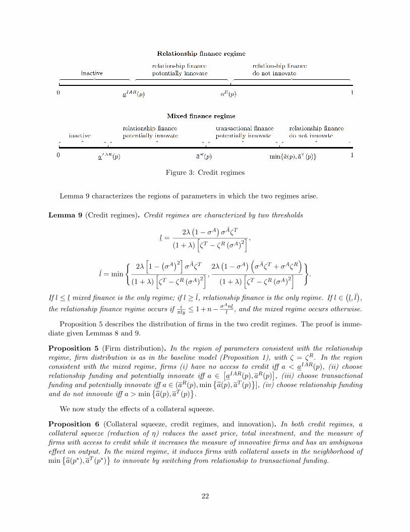
Figure 3: Credit regimes

Lemma 9 characterizes the regions of parameters in which the two regimes arise.

Lemma 9 (Credit regimes). Credit regimes are characterized by two thresholds

l =2λ(1− σA

)σAζT

(1 + λ)[ζT − ζR (σA)2

] ,

l = min

{2λ[1−

(σA)2]

σAζT

(1 + λ)[ζT − ζR (σA)2

] , 2λ(1− σA

) (σAζT + σAζR

)(1 + λ)

[ζT − ζR (σA)2

] }.

If l ≤ l mixed finance is the only regime; if l ≥ l, relationship finance is the only regime. If l ∈(l, l),

the relationship finance regime occurs if iπly ≤ 1 +n− σAnl

l , and the mixed regime occurs otherwise.

Proposition 5 describes the distribution of firms in the two credit regimes. The proof is imme-diate given Lemmas 8 and 9.

Proposition 5 (Firm distribution). In the region of parameters consistent with the relationshipregime, firm distribution is as in the baseline model (Proposition 1), with ζ = ζR. In the regionconsistent with the mixed regime, firms (i) have no access to credit iff a < aIAR(p), (ii) chooserelationship funding and potentially innovate iff a ∈

[aIAR(p), aR(p)

], (iii) choose transactional

funding and potentially innovate iff a ∈ (aR(p),min{a(p), aT (p)

}], (iv) choose relationship funding

and do not innovate iff a > min{a(p), aT (p)

}.

We now study the effects of a collateral squeeze.

Proposition 6 (Collateral squeeze, credit regimes, and innovation). In both credit regimes, acollateral squeeze (reduction of η) reduces the asset price, total investment, and the measure offirms with access to credit while it increases the measure of innovative firms and has an ambiguouseffect on output. In the mixed regime, it induces firms with collateral assets in the neighborhood ofmin

{a(p∗), aT (p∗)

}to innovate by switching from relationship to transactional funding.

22

In the relationship finance regime, collateral-rich firms innovate within their credit relationships.In the mixed regime, instead, since min

{a(p∗), aT (p∗)

}is negatively related to the asset price, after

the drop in η collateral-rich firms innovate by switching to transactional funding. This can haveimplications for output. In fact, since the recovery value of collateral assets is higher within creditrelationships, the switch to transactional funding increases liquidation costs. If these costs areassumed to be at least partially a real resource loss, this adds to the effects on output of theinvestment decline and of the increase in innovation.

Discussion. One may argue that some types of lenders, though at a disadvantage in liquidatingcollateral assets (like the transactional lenders in the above extension), have the ability to boost thesuccess probability of innovations. This might be the case for venture capitalists, which allegedlyhave less experience on mature, established technologies but have also special expertise in acquiringinformation about new technologies and asset vintages. Although, as noted, our model does notfocus on venture capital finance, we could capture this scenario by assuming that for transactionallenders ζT > ζR and σAT < σAR.23 The analysis and results are similar to the case with only ζT >ζR. Higher probability of innovation further reduces entrepreneurs’ collateral maintenance whenthey borrow from transactional lenders, as collateral assets are less likely to be useful. The rankingsaIAR(p) < aIAT (p) and aR(p) < aT (p) are further reinforced. Therefore, under an assumptionsimilar to A4, we again obtain the rankings of thresholds aIAR(p) < aIAT (p) < aR(p) < aT (p).

The entrepreneurs make decisions on which lender to borrow from and whether to adopt aninnovative plan. Again, collateral-poor firms with a < aIAR(p) cannot obtain credit, even if theychoose relationship funding; collateral-rich firms with a > aT (p) cannot innovate, even if theychoose transactional funding. Since relationship funding is cheaper, they choose to borrow fromrelationship lenders. Firms with a ∈

(aIAR(p), aIAT (p)

)can only borrow from relationship lenders

and innovate. Firms with a ∈[aIAT (p), aR(p)

]can borrow from both types of lenders and in-

novate. The trade-off is that relationship lenders induce lower innovation probability but alsolower maintenance costs of mature assets. Assuming that the advantage of lower maintenancecost dominates, firms with a ∈

[aIAT (p), aR(p)

]would all choose relationship lenders. Firms with

a ∈(aR(p), aT (p)

)] face the choice between transactional lenders that facilitate innovation versus

relationship lenders that hinder innovation. Similar as in Lemma 8, either the mixed finance regimeor the relationship finance regime could occur.

7.2 Managerial firms

In the baseline model, we have considered entrepreneurial firms. In this section, we extend thebaseline model to managerial firms and investigate the interaction between lenders’ inertia and aform of technological inertia inside borrowing firms. The source of borrowers’ inertia is the higherrisk of failure that the new technology can entail relative to the mature technology.

We model technological inertia inside borrowing firms building on the extant literature onagency conflicts in managerial firms (see, e.g., Jensen and Meckling, 1976, for a discussion). Wenow posit that the economy is also populated by a continuum of managers of measure larger thanone. Managers have no endowment and have the same utility as entrepreneurs and investors.In a firm the implementation of a project now requires a manager, who faces an effort (or anopportunity) cost e for working for the firm. On date 2, the manager can carry out a non-verifiablecostless action that facilitates innovation: if the manager and the lender both take actions, thenthe probability of innovation increases from 1− σA to 1− σA. To highlight managers’ aversion toinnovation due to higher riskiness of the new technology, we now let the success probability πn of

23We assume that σAT = σAR = σA, so the probability of innovation is the same when lenders do not take actions.

23

the new technology be lower than the success probability π of the mature one (though, consistentwith the baseline model, πny(1 + n) > πy).

A manager’s compensation package comprises a wage w if the project succeeds and the firmremains in business, plus a possible bonus wn in the event the new technology is successfullyadopted. In case of project failure, the manager loses his job and obtains zero. With a flatcompensation (i.e., w > 0, wn = 0), the manager would prefer retaining the mature technologywith its higher success probability in order to minimize the risk of losing his job. To preventthis, the entrepreneur needs to pledge part of the higher output of the new technology as a bonus(wn > 0) to the manager. Assuming that he breaks a tie in favor of innovation, the incentiveconstraint under which the manager prefers facilitating the new technology reads

(1− σA)πn(w + wn) + σAπw ≥ (1− σA)πn(w + wn) + σAπw, (10)

or, rearranging,

wn ≥(π − πn)

πnw. (11)

The manager’s bonus reduces the output pledgeable to the lender in case of successful adoption ofthe new technology. Thus, the entrepreneur now faces a tension between the need to incentivize thelender and the need to incentivize the manager. Lemma 10 solves for the collateral asset thresholdbelow which a firm has no access to credit and the threshold above which a firm does not innovate.The lemma compares these thresholds with those in the absence of managers’ moral hazard (forexample, if managers worked for firms but did not affect innovation).

Lemma 10 (Managers’ and lenders’ inertia). There exists a feasible contract that induces botha lender and a manager to facilitate innovation if and only if the entrepreneur’s collateral assetssatisfy a ∈

[a′IA(p), a′(p)

], where

a′IA(p) =ζ[i+ e− (1− σA)πnl(1 + n)y − σAπly]

(σA)2(1− π)2λ(1− λ)p

a′(p) =ζ[πnly(1 + n)− e− i]σAσA(1− π)2λ(1− λ)p

.

Absent managers’ moral hazard, the threshold above which firms do not innovate would equal

a′′(p) ≡ζ[πnly(1 + n)− πne

(1−σA)πn+σAπ− i]

σAσA(1− π)2λ(1− λ)p> a′(p), (12)

while the threshold below which firms do not obtain credit would equal a′′IA(p) = a′IA(p).

Henceforth, we maintain assumptions analogous to A1-A3 to guarantee that in this extendedenvironment a positive measure of firms (but not all firms) obtain credit (0 < a′IA(p) < 1) andthat a positive measure of funded firms potentially innovate (a′IA(p) < a′(p)).

Lemma 10 shows that, for a given asset price, the region of collateral values in which techno-logical inertia arises is now larger (a′(p) < a′′(p)). In particular, an entrepreneur with a > a′(p)cannot simultaneously satisfy the lender’s and the manager’s incentive constraints, so that eitherthe lender or the manager do not have the incentive to facilitate the innovation. To complete theanalysis, however, we need to account for the general equilibrium effects through the asset price.

24

Proposition 7 (Firms’ innovation). The measure of innovative firms is lower in the presence ofmanagers’ moral hazard than in its absence.

As shown in Lemma 10, in this extended environment in which both lenders and managerscan engage in technological inertia the measure of innovative firms tends to be lower. Since thenew technology succeeds with a lower probability (πn < π), this implies that a larger measure offirms remain in business and a smaller measure of firms fail. The resulting higher net demand forliquidated assets induces a higher asset price, further exacerbating technological inertia (rememberthat a′(p) is negatively related to p). Thus, there is both a direct negative effect and an indirect,general equilibrium negative effect (through asset prices) on the measure of innovative firms.

It is immediate that the results on the effects of a collateral squeeze (drop in η) carry throughto this extended environment. Moreover, a given drop in the asset price boosts the measure ofinnovative firms more than in the baseline model (see the proof of Proposition 7).

7.3 Other extensions

In the Supplement of the paper, we present other extensions and robustness checks of the baselineresults. First, we study the effects of a drop in the probability of success of projects, rather thanthe effects of a collateral squeeze. We then investigate a scenario in which lenders exert control overthe success probability of projects, rather than exerting control over the probability of innovationopportunities.24 Finally, we examine the case in which the success probability of the new technologyis higher or lower than the success probability of the mature one. We show that in these variousalternative scenarios the baseline results of the analysis carry through, with opportune revisitationsof the parametric assumptions. Indeed, in the Supplement we show that agents’ decisions are thesame as in the baseline model, when parameters are chosen in a specific way. We refer the readerto the Supplement for more details.

8 Conclusion

This paper has studied a credit crunch triggered by a drop in collateral asset values in an economywhere firms can adopt new technologies or retain less productive technologies. In our economy,lenders hinder the innovation of collateral-rich firms to preserve the value of their informationon mature technologies. By depressing the price of collateral assets, a negative collateral shocksqueezes collateral-poor firms out of the credit market but fosters the innovation of collateral-richfirms. The analysis reveals that credit and asset market policies such as those implemented duringthe recent credit crisis promote investment but may slow down innovation.

The paper leaves important questions open for future research. First, while the model can helpdisentangle the effects of a credit crunch on technological change, it cannot offer predictions ontheir magnitude. A priority is to cast the analysis into a dynamic general equilibrium environmentand study the quantitative relevance of the effects. Second, in our economy, following negativecollateral shocks collateral-poor firms lose access to credit while collateral-rich firms switch to moreproductive technologies. Thus, the cross-sectional dispersion of innovation increases. Interestingly,this is reminiscent of the finding of Bloom, Floetotto, Jaimovich, Saporta-Eksten and Terry (2018)that during recessions the cross-sectional dispersion of output rises. An objective for future researchis to dig deeper into the cross-sectional effects of a credit crunch on innovation and output.

24We also show robustness to assuming that the lender has partial ability to liquidate the assets of the newtechnology.

25

References

Aghion, P. and P. Bolton (1992) “An incomplete contracts approach to financial contracting,”Review of Economic Studies 59, 3, 473–494.

Allen, F. and D. Gale (2001) Comparing Financial Systems. MIT Press, Cambridge, MA.

Altman, I., Haldeman R. G. and P. Narayanan (1977) “ZETA analysis. A new model to identifybankruptcy risk of corporations,” Journal of Banking & Finance 1, 1, 29–54.

Beck, T., Degryse, H., De Haas, R. and N. van Horen (2018) “When arm’s length is too far.Relationship banking over the credit cycle,” Journal of Financial Economics 127, 1, 174–196.

Berger, A. N. and G. F. Udell (2002) “Small business credit availability and relationship lending:The importance of bank organisational structure,” Economic Journal 102, 2, 32–53.

Berlin, M. and A. Butler (2002) “Collateral and competition,” Working paper 02-22, Federal Re-serve Bank of Philadelphia.

Bhattacharya, S. and G. Chiesa (1995) “Proprietary information, financial intermediation, andresearch incentives,” Journal of Financial Intermediation 4, 4, 328–357.

Bloom, N., Floetotto, M., Jaimovich, N., Saporta-Eksten, I. and S. J. Terry (2018) “Really uncer-tain business cycles,” Econometrica, forthcoming.

Braun, M. (2005) “Financial contractability and asset hardness,” Working Paper, UniversidadAdolfo Ibanez.

Buera and Moll (2015) “Aggregate implications of a credit crunch: The importance of heterogene-ity,” American Economic Journal: Macroeconomics 7, 3, 1–42.

Caballero, R. and M. Hammour (2005) “The costs of recessions revisited: a reverse-liquidationistview,” Review of Economic Studies 72, 2, 313–341.

Caballero, R.J. and Hammour M. (1994) “The cleansing effect of recessions,” American EconomicReview 84, 5, 1350–68.

Calomiris, C., Larrain, M., Liberti J. and J. Sturgess (2017) “How collateral laws shape lendingand sectoral activity,” Journal of Financial Economics 123, 1, 163–188.

Carpenter, R.J. and B. Petersen (2002) “Capital market imperfections, high-tech investment, andnew equity financing,” Economic Journal 102, 2, 54–72.

Catherine, S., T. Chaney, Z. Huang, D. Sraer and D. Thesmar (2017) “Aggregate effects of collateralconstraints: Evidence from a structural estimation,” Working Paper, MIT.

Cincera, M., Cozza, C., Tubke, A. and P. Voigt (2012) “Doing R&D or not (in a crisis), that is thequestion...,” European Planning Studies 20, 9, 1525–1547.

Dell’ Ariccia, G. and P. Garibaldi (2001) “Bank lending and interest rate changes in a dynamicmatching model,” International Monetary Fund, Working Paper 98/93.

Den Haan, W. J., G. Ramey and J. Watson (2003) “Liquidity flows and fragility of businessenterprises,” Journal of Monetary Economics 50, 6, 1215–1241.

26

Diamond, D. and R. Rajan (2001) “Liquidity risk, liquidity creation and financial fragility: a theoryof banking,” Journal of Political Economy 109, 2, 287–327.

European Commission (2012) “EU R&D scoreboard - The 2012 EU industrial R&D investmentscoreboard,” Joint Research Centre, Directorate-General for Research and Innovation, EuropeanCommission, Brussels.

Field, A. (2011) A Great Leap Forward: 1930s Depression and U.S. Economic Growth. Yale Uni-versity Press.

Garcia-Macia, D. (2017) “The financing of ideas and the great deviation. Working Paper No.17/176, International Monetary Fund, Washington, D.C.

Gertler, M. and P. Karadi (2011) “A model of unconventional monetary policy,” Journal of Mone-tary Economics 58, 1, 17–34.

Gertler, M. and N. Kiyotaki (2010) “Financial intermediation and credit policy in business cycleanalysis,” in: B. M. Friedman and M. Woodford, eds., Handbook of Monetary Economics 1, 3, pp.547–599.

Gertler, M. and N. Kiyotaki (2015) “Banking, liquidity, and bank runs in an infinite horizoneconomy,” American Economic Review 105, 7, 2011–43.

Gilchrist, S., J. W. Sim and E. Zakraj (2014) “Uncertainty, financial frictions, and investmentdynamics,” NBER Working Paper No. 20038.

Goodacre, A. and I. Tonks (1995) “Finance and technological change,” in P. Stoneman, ed.: Hand-book of the economics of innovation and technological change. Blackwell, Oxford.

Guiso, L. and R. Minetti (2010) “The structure of multiple credit relationships: Evidence fromU.S. firms,” Journal of Money, Credit and Banking 42, 6, 1037–1071.

Habib, M. A. and D. B. Johnsen (1999) “The financing and redeployment of specific assets,” Journalof Finance 54, 2, 693–720.

Hall, B. (2011) “R&D in the crisis,” OECD Lecture, Workshop on R&D and innovation in thecurrent macroeconomic climate, OECD, Paris, France.

Hall, B. and B. Khan (2003) “Adoption of new technology,” in: Jones, D.C. (Ed.), New EconomyHandbook. Elsevier Science, Amsterdam, pp. 230–251.

Holmstrom, B., and J. Tirole (1997) “Financial intermediation, loanable funds and the real sector,”Quarterly Journal of Economics 112, 3, 663–691.

ILO (2001) “Collateral, collateral law and collateral substitutes,” Social Finance Working PaperNo. 26, Geneva.

Jensen, M. J. and W. H. Meckling (1976) “Theory of the firm: Managerial behavior, agency costsand ownership structure,” Journal of Financial Economics 3, 4, 305–360.

Kim, H. and H. Kung (2017) “The asset redeployability channel: How uncertainty affects corporateinvestment,” Review of Financial Studies 30, 1, 245–280.

27

Kiyotaki, N. and J. Moore (1997) “Credit cycles,” Journal of Political Economy 105, 2, 211–48.

Lorenzoni, G. (2008) “Inefficient credit booms,” Review of Economic Studies 75, 3, 809–833.

OECD (2009) Policy Responses to the Economic Crisis: Investing in Innovation for Long-TermGrowth. Paris, France.

Rajan, R. (1992) “Insiders and outsiders: the choice between informed and arm’s length debt,”Journal of Finance 47, 4, 1367–1400.

Rajan, R. and L. Zingales (2001) “Financial systems, industrial structure, and growth,” OxfordReview of Economic Policy 17, 4, 467–482.

Ramey, G. (2004) “Financial intermediation in a restructuring economy,” Unpublished workingpaper, University of California San Diego.

Shourideh, A. and A. Zetlin-Jones (2017) “External financing and the role of financial frictions overthe business cycle: Measurement and theory,” Journal of Monetary Economics 92, 1–15.

Udell, G. (2004) Asset-Based Finance: Proven Disciplines for Prudent Lending. Commercial Fi-nance Association, New York.

Voigt, P. and P. Moncada-Paterno-Castello (2009) “The global economic and financial downturn:What does it imply for firms’ R&D strategies?” IPTS Working Paper No. 12/2009, EuropeanCommunities.

Wang, Y. (2017) “Debt market friction, firm-specific knowledge capital accumulation and macroe-conomic implications.” Review of Economic Dynamics 26, 19–39.

Appendix A

This Appendix A contains: i) details on data sources and definitions for the empirical analysis;ii) Appendix Tables A.1 and A.2 for the empirical analysis.

Data Sources and Definitions

The data collection for EFIGE was performed through a survey carried out by a professional con-tractor. The questionnaire covers six areas: firm ownership structure; workforce characteristics;investment, technological innovation, R&D (and related financing); export and internationaliza-tion; market structure and competition; financial structure and bank-firm relationships. To ensurestatistical representativeness, the data set was built so as to fulfill two main criteria. First, theavailability of an adequately large target sample of firms, initially set at around 3,000 firms for largecountries (France, Germany, Italy, Spain and the UK), and about 500 firms for smaller countries(Austria and Hungary). Second, a proper stratification of the sample to ensure representativeness ofthe collected data ex ante and ex post for each country, considering in particular three dimensions:sector composition, regions and size classes.

The EFIGE survey provides information on innovation activities and on the impact of the finan-cial crisis on such activities. For measuring innovation activities, we use and combine informationfrom three questions: 1) During 2009, has your firm decided to postpone investments in innova-tion? (Yes/No); 2) Always referring to the last year (2009), the range of products that your firm

28

has decided to offer has (relative to past years): (a) Been widened; (b) Remained the same; (c)Been reduced; 3) On average in the last three years did the firm carry out product innovation,that is, introduction of a good which is either new or significantly improved with respect to itsfundamental characteristics (the innovation should be new to the market)? (Yes/No).

Starting from these questions, we construct two variables: “engagement in innovations in 2008-2009” is a dummy equal to one if the firm answers Yes to question 3), zero otherwise; “start oracceleration of non-marginal innovations in 2008-2009” is a dummy equal to one if the firm answersNo to question 1), a) to question 2) and Yes to question 3), zero otherwise.

Data on fixed and total assets are from firms’ balance sheet information (BvD-Amadeus).Further, in the following survey question, firms are requested to specify the type of information

they normally provide to their main bank in the screening and monitoring process. The questionreads out as follows: “Which type of information does the bank normally use/ask to assess yourfirm’s creditworthiness? (a) collateral (0/1); (b) balance sheet information (0/1); (c) interviewswith management on firm’s policy and prospects (0/1); (d) business plan and firms’ targets (0/1);(e) historical records of payments and debt service (0/1); (f) brand recognition (0/1); (g) other(0/1).” Starting from this categorization, following Berger and Udell (2006), we build a dummyvariable “Emphasis on Collateral” that equals one if the firm answers yes to a), and zero otherwise.

Relationship length is defined as the number of years the firm has been doing business with itsmain bank. The variable “Bank Involvement in Investments Finance” is based on a survey questionasking the firms the percentage of investments that was financed with bank credit. We construct adummy that equals 1 if this percentage is higher than the sample median, and zero otherwise.

Labor productivity of a firm is measured as value added per worker.Leverage is defined as the total liabilities of the firm divided by total assets. As noted in the

text, we also construct the ratios of bank debt over total liabilities and of short-term bank debtover total liabilities.

Cash flow of the firm is available from the Amadeus database. Liquidity ratio is defined as theratio of the value of cash and cash-equivalent instruments of the firm over total assets of the firm.

The sectoral measure of asset tangibility is obtained from Braun (2005).The alternative dependent variable of columns 3-6 of Table A.2 is a dummy that takes the value

of one if a firm undertook non-marginal innovation activities, did not postpone innovation, and, ontop of this, applied for a patent in 2008-2009 or purchased foreign R&D and engineering services.

ROA is the return on assets, defined as the EBIT (earning before interests and taxes) over totalassets. The Z-score is adapted from Altman (1977) to account for the case of non-listed firms. Itis obtained as a linear combination of business ratios, weighted by coefficients. In particular, itincludes current assets minus current liabilities, over total assets; retained earnings over total assets;earnings before interests and taxes, over total assets; book value of equity over total liabilities; andsales over total assets.

The proxy for exit is constructed from the Orbis and Amadeus databases, using information onthe last year in which firms report information and status of the firms in the last year of report.The solvency ratio used in Supplementary Table S.4 is from Orbis and Amadeus.

29

Tab

leA

.1:

Rob

ust

nes

sT

ests

.R

ole

ofF

irm

Lev

erag

e,D

ebt

and

Cas

h

30

Tab

leA

.2:

Rob

ust

nes

sT

ests

.A

lter

nat

ive

Pro

xie

s;R

ole

ofF

irm

Pro

fita

bil

ity

and

Dis

tres

s

31

Appendix B

This Appendix B contains the main proofs for the theoretical model.

Proof of Lemma 1

If an entrepreneur adopts the innovative plan, and the lender exerts action, the entrepreneur choosesmaintenance effort to maximize:

maxµIA

(1− π)(1− λ)σAµIApa−ζ(µIA

)22

pa.

From the first order condition, we solve for µIA = (1−π)(1−λ)σA

ζ .If an entrepreneur adopts the innovative plan, while the lender chooses inaction, the en-

trepreneur chooses maintenance effort to maximize:

maxµIA

(1− π)(1− λ)σAµIApa−ζ(µIA

)2

2pa.

Therefore, µIA = (1−π)(1−λ)σA

ζ .If an entrepreneur does not adopt an innovative plan, the entrepreneur solves the problem:

maxµI

(1− π)(1− λ)µIpa−ζ(µI)2

2pa.

Therefore, µI = (1−π)(1−λ)ζ .

Proof of Lemma 2

The incentive compatibility constraint for the lender is

(1− σA)πrIn + σA[πrIm + λ(1− π)µIApa

]≥ (1− σA)πrIn + σA

[πrIm + λ(1− π)µIApa

], (13)

which implies equation (1). The participation constraint for the lender is

(1− σA)πrIn + σA[πrIm + λ(1− π)µIApa

]≥ i. (14)

Due to limited commitment, the lender can at most pledge l fraction of output. Therefore,

rIn ≤ ly(1 + n), and rIm ≤ ly.

As shown in Figure A.1, for the existence of a feasible contract, the point (rIm, rIn) = (ly, ly(1 + n))

must lie in the shaded area. Therefore, (ly, ly(1 + n)) must satisfy two conditions: (i) it must lieabove the PC, i.e.,

(1− σA)πly(1 + n) + σA[πly + λ(1− π)µIApa

]≥ i,

32

from which we can solve for

a ≥ ζ[i− πly(1 + n− σAn)]

(σA)2(1− π)2λ(1− λ)p≡ aIA(p);

(ii) it is above the intersection of IC and PC, i.e.,

i

π+σAσA(1− π)2λ(1− λ)pa

πζ≤ ly(1 + n),

from which we can solve for

a ≤ ζ[πly(1 + n)− i]σAσA(1− π)2λ(1− λ)p

≡ a(p).

Figure A.1: IC and PC of the lender

Proof of Lemma 3

If an entrepreneur adopts an innovative plan but the lender hinders innovation, the lender’s par-ticipation constraint is

(1− σA)πrIn + σA[πrIm + λ(1− π)µIApa

]≥ i. (15)

Using the fact that rIn ≤ ly(1 + n), and rIm ≤ ly, we can derive aIA(p) in Lemma 3.If an entrepreneur does not adopt an innovative plan, the lender’s participation constraint is

πrIm + λ(1− π)µIpa ≥ i. (16)

Using the fact that rIm ≤ ly, we can derive aI(p) in Lemma 3.

33

Proof of Lemma 4

To show that aIA(p) < a(p),

a(p)

aIA(p)> 1⇔ σA[πly(1 + n)− i]

σA[i− πly(1 + n− σAn)]> 1⇔ i

πly< 1 + n− σAσAn

σA + σA.

The last inequality holds under assumption A1, as 11+σA

< 1− σAσA

σA+σA, when σA, σA ∈ (0, 1).

To show that aIA(p) < aIA(p) < a(p),

aIA(p)

aIA(p)> 1⇔ (σA)2[i− πly(1 + n− σAn)]

(σA)2[i− πly(1 + n− σAn)]> 1⇔ i

πly< 1 + n− σAσAn

σA + σA,

anda(p)

aIA(p)> 1⇔ σA[πly(1 + n)− i]

σA[i− πly(1 + n− σAn)]> 1⇔ i

πly< 1 + n− σAσAn

σA + σA.

Both inequalities hold under assumption A1, as 11+σA

< 1− σAσA

σA+σA, when σA, σA ∈ (0, 1).

To prove that aI(p) > aIA(p) and aI(p) < a(p),

aI(p)

aIA(p)> 1⇔ (σA)2 (i− πly)

i− πly(1 + n− σAn)> 1⇔ i

πly< 1 +

n

1 + σA.

anda(p)

aI(p)> 1⇔ πly(1 + n)− i

σAσA (i− πly)> 1⇔ i

πly< 1 +

n

1 + σAσA.

The last inequality holds under assumption A1, as 11+σA

< 11+σAσA

, when σA ∈ (0, 1).

To prove the last part of the lemma,

aIA(p) > 0⇔ ζ[i− πly(1 + n− σAn)]

(σA)2(1− π)2λ(1− λ)p> 0⇔ i

πly> 1 + n− σAn.

Proof of Lemma 5

Firms with a ∈[aIA(p), aI(p)

)have no option but to innovate in order to obtain credit. For a firm

with a ∈[aI(p), a(p)

], if it chooses an innovative plan, the lender will facilitate innovation. Such a

firm chooses an innovative plan if and only if

(1− σA)π[(1 + n)y − rIn

]+ σA

[π(y − rIm

)+ (1− π) (1− λ)µIApa

]−ζ(µIA

)22

pa

≥π(y − rIm

)+ (1− π)(1− λ)µIpa−

ζ(µI)2

2pa. (17)

Using the lenders’ participation constraints (14) and (16), and the entrepreneurs’ choice of main-tenance efforts in Lemma 1, we can get a ≤ 2ζπny

(1−π)2(1−λ2)(1+σA)p≡ a∗A(p). Under the assumption

l < 2λ1+λ and assumptions A1, we have a∗A(p) > aI(p). To see this,

a∗A(p)

aI(p)> 1⇔ i

πly< 1 +

2λ

l(1 + λ) (1 + σA).

34

The latter holds when l < 2λ1+λ and assumptions A1 holds.

For a firm with a > a(p), if it chooses an innovative plan, the lender will not facilitate innovation,and innovation opportunities arrive with lower probability. Such a firm chooses an innovative planif and only if

(1− σA)π[(1 + n)y − rIn

]+ σA

[π(y − rIm

)+ (1− π) (1− λ)µIApa

]−ζ(µIA

)2

2pa

≥π(y − rIm

)+ (1− π)(1− λ)µIpa−

ζ(µI)2

2pa. (18)

Using the lenders’ participation constraints (15) and (16), and the entrepreneurs’ choice of main-tenance efforts in Lemma 1, we can get a ≤ 2ζπny

(1−π)2(1−λ2)(1+σA)p≡ a∗A(p). As σA > σA, a∗A(p) <

a∗A(p). Depending on the ranking of a∗A(p), a∗A(p), and a(p), we have the following three cases:

(i) If iπly ≤ 1 + n − 2λnσAσA

l(1+λ)(1+σA), then a∗A(p) < a∗A(p) ≤ a(p). An entrepreneur chooses an

innovative plan if a ∈[aIA(p), a∗A(p)

].

(ii) If 1 + n − 2λnσAσA

l(1+λ)(1+σA)< i

πly < 1 + n − 2λnσAσA

l(1+λ)(1+σA), then a∗A(p) < a(p) < a∗A(p). An

entrepreneur chooses an innovative plan if a ∈[aIA(p), a(p)

].

(iii) If iπly ≥ 1 + n − 2λnσAσA

l(1+λ)(1+σA), then a(p) ≤ a∗A(p) < a∗A(p). An entrepreneur chooses an

innovative plan if a ∈[aIA(p), a∗A(p)

].

Proof and Lemma 6

Equating demand and supply gives[1− aIA(p)

]π

(1− p

ηθ

)=

1

2(1− π)

[1− aIA(p)2

]which can be rewritten as

π

ηθp2 − 3π − 1

2p+

ζ[i− πly

(1 + n− σAn

)]2 (σA)2 (1− π)λ(1− λ)

= 0.

We obtain

p∗ =ηθ

2π

3π − 1

2±

[(3π − 1

2

)2

− 2π

ηθ

ζ[i− πly

(1 + n− σAn

)](σA)2 (1− π)λ(1− λ)

] 12

.

We restrict the parameters to ensure that aIA(p) < 1 and that there is a unique positive equilibriumprice. This implies that aIA(p−) > 1 and aIA(p+) < 1. Substituting for the price, both hold whenassumption A3 holds.

Proof of Proposition 1

The proof directly follows from Lemmas 1-6. There are two cases to be considered. First, a(p∗) ≥ 1,

which occurs whenever p∗ ≤ ζ[πly(1+n)−i]σAσA(1−π)2λ(1−λ)

, i.e.,

ηθ ≤ ζ[πly(1 + n)− i]σAσA(1− π)2λ(1− λ)

[3π − 1

2π− (1− π)σA

2πσAi− πly

(1 + n− σAn

)πly(1 + n)− i

]−1

.

35

In this case, all firms with collateral a > aIA(p∗) have access to credit and potentially innovate.

Second, a(p∗) < 1, which occurs whenever p∗ > ζ[πly(1+n)−i]σAσA(1−π)2λ(1−λ)

, i.e.,

ηθ >ζ[πly(1 + n)− i]

σAσA(1− π)2λ(1− λ)

[3π − 1

2π− (1− π)σA

2πσAi− πly

(1 + n− σAn

)πly(1 + n)− i

]−1

.

In this case, all firms with collateral a ∈[aIA(p∗), a(p∗)

]have access to credit and potentially

innovate, and all firms with collateral a > a(p∗) have access to credit but do not innovate.

Proof of Proposition 2

Given (4), it is straightforward that ∂p∗

∂η > 0. The investment change is computed by multiplying i

by the change in the measure of firms obtaining credit, C = 1− aIA(p∗):

∂I

∂η= i

∂C

∂η= −i∂a

IA(p∗)

∂p∗∂p∗

∂η> 0.

If (5) holds, the measure of firms that innovate equals that of firms with access to credit: C = N .Hence, ∂N

∂η > 0. If (5) does not hold, N = a(p∗)− aIA(p∗) and

∂N

∂η= −a(p∗)− aIA(p∗)

p∗∂p∗

∂η.

Assumption A2 implies that ∂N∂η < 0.

Consider now output. If (5) holds, letting L denote the measure of investors,

Y = ωL+ C[πy(1 + n− nσA

)− i]

+ πC

∫ θ

p∗η

ηθ

θdθ.

The second term is increasing in η because ∂C∂η > 0. We show the third term is also increasing in η,

πC

∫ θ

p∗η

ηθ

θdθ = πC

η2θ2 − p∗2

2ηθ=ηθ

2πC

(1− p∗

ηθ

)(1 +

p∗

ηθ

)=ηθ

2D(p∗)

(1 +

p∗

ηθ

)=ηθ

2S(p∗)

(1 +

p∗

ηθ

).

It is straightforward to show that ∂S(p∗)∂η > 0 and

∂ p∗η

∂η > 0. Therefore, the third term is alsoincreasing in η. If (5) does not hold,

Y = ωL+ C

{π

[1 +

N

C(1− σA)n

]y − i

}+ πC

∫ θ

p∗η

ηθ

θdθ.

An increase in η raises output iff

∂C

∂η(πy − i) + π

∂

(C∫ θp∗η

ηθθdθ

)∂η

> −∂N∂η

π(1− σA)ny.

36

The Following Supplement is Not Intended forPublication.

Supplement. Not for Publication

This supplement contains:Section A) technical proofs omitted from the main text;Section B) robustness analysis: a case in which the new technology has higher success prob-

ability than the mature technology (Section B.1); a case in which the new technology has lowersuccess probability than the mature technology (Section B.2); a case in which the assets of the newtechnology have positive liquidation value (Section B.3);

Section C) further extensions of the baseline setting: a case in which the lender has control overthe probability of project success (Section C.1); a case of a shock given by a drop in the probabilityof project success π (Section C.2);

Section D) numerical experiments;Section E) supplementary empirical figures and tables: supplementary Tables S.3 and S.4 for the

empirical analysis, as well as Figure S.5 for the joint distribution of firms’ collateral and innovation.

A Technical Proofs

Proof of Lemma 7

The marginal firm that obtains credit has collateral equal to aIA(p∗). The social value of thismarginal firm is

V = (1− σA)[πy(1 + n) + (1− π)ηθaIA(p∗)

]+ σA

[πy + (1− π)ηθaIA(p∗)

]− i,

where θ is the marginal buyer of resale assets. The maintenance costs are assumed to be transfers,so they are not subtracted from the social value. We now show that the social value of the marginalfirm is positive. The participation constraint of the marginal firm’s lender implies that

(1− σA)πly(1 + n) + σA[πly + λ(1− π)µIAp∗aIA(p∗)

]=(1− σA)πly(1 + n) + σA

[πly + λ(1− π)µIAηθaIA(p∗)

]= i.

Therefore,

V = (1−σA)[π(1− l)y(1 + n) + (1− π)ηθaIA(p∗)

]+σA

[π(1− l)y + (1− π)ηθaIA(p∗)

(1− λµIA

)]> 0.

The last inequality holds both because l < 1 (i.e., the social planner would account for the outputnot pledgeable to investors) and because the social planner would internalize the asset liquidationreturns of the new technology (which are a transfer). It follows that in the allocation chosen bythe social planner, a positive measure of firms with a < aIA(p∗) would invest.

In the social planner’s problem, all funded firms will take the innovative plan. This is because(i) since the liquidation costs are a transfer, in the event of project failure the asset liquidationreturns of the two technologies are equal; (ii) in the event of project success the output of the newtechnology exceeds that of the mature since y(1 + n) > y.

Supp.Page 1

Proof of Proposition 3

The asset demand and supply are

D(p) =[1− aIA(p)

]π

(1− p− τ

ηθ

)and S(p) =

1

2(1− π)

[1− aIA(p)2

].

Equating D(p) and S(p) and solving for p,

p∗(τ) =τ

2+ηθ

2π

3π − 1

2±

[(3π − 1

2+πτ

ηθ

)2

− 2π

ηθ

ζ[i− πly

(1 + n− σAn

)](σA)2 (1− π)λ(1− λ)

] 12

.

To ensure that there exists a unique positive equilibrium price, we need aIA(p+) < 1 and aIA(p−) >1. These hold whenever

ηθ

(π − 1

2

)>π

2

[ζ[i− πly

(1 + n− σAn

)](σA)2 (1− π)2 λ(1− λ)

− τ

]and the unique price is

p∗(τ) =τ

2+ηθ

2π

3π − 1

2+

[(3π − 1

2+πτ

ηθ

)2

− 2π

ηθ

ζ[i− πly

(1 + n− σAn

)](σA)2 (1− π)λ(1− λ)

] 12

.

Clearly, ∂p∗

∂τ > 0. Thus,

∂C(τ)

∂τ= −∂a

IA(p∗)

∂p∗∂p∗(τ)

∂τ> 0.

If (7) holds, the measure of innovative firms equals that of firms with access to credit. Hence,∂N(τ)∂τ > 0. To show that ∂Y/∂τ > 0, note that if (7) holds,

Y = ωL+ C[πy(1 + n− nσA

)− i]

+ πC

∫ θ

p∗−τη

ηθ

θdθ.

The second term increases in τ because ∂C∂τ > 0. It remains to show that the third term also

increases in τ . If ∂(p∗ − τ)/∂τ ≤ 0, then it immediately follows that πC∫ θp∗−τη

ηθθdθ increases in τ .

If ∂(p∗ − τ)/∂τ > 0, note that

πC

∫ θ

p∗−τη

ηθ

θdθ = πC

η2θ2 − (p∗ − τ)2

2ηθ=ηθ

2πC

(1− p∗ − τ

ηθ

)(1 +

p∗ − τηθ

)=ηθ

2D(p∗)

(1 +

p∗ − τηθ

)=ηθ

2S(p∗)

(1 +

p∗ − τηθ

).

Because ∂S(p∗)∂τ = ∂S(p∗)

∂p∗∂p∗

∂τ > 0, ηθ2 S(p∗)

(1 + p∗−τ

ηθ

)increases in τ , and so does πC

∫ θp∗−τη

ηθθdθ.

Therefore, whether ∂(p∗ − τ)/∂τ ≤ 0 or not, we have shown that the third term is also increasingin τ .

If (7) does not hold, N = aIA(p∗)− a(p∗) and

∂N(τ)

∂τ= −a(p∗)− aIA(p∗)

p∗∂p∗(τ)

∂τ< 0.

Supp.Page 2

Output equals

Y = ωL+ C

{π

[1 +

N

C(1− σA)n

]y − i

}+ πC

∫ θ

p∗−τη

ηθ

θdθ.

An increase in τ raises output iff

∂C

∂τ(πy − i) + π

∂

(C∫ θp∗−τη

ηθθdθ

)∂τ

> −∂N∂τ

π(1− σA)ny.

Proof of Proposition 4

The asset demand and supply are

D(p) = (1− aG)π

(1− p

ηθ

)and S(p) =

1

2(1− π)

(1− a2

G

).

Equating

p∗(aG) =ηθ

2π[3π − 1− (1− π) aG] .

We let aIA(p∗) < 1, which holds whenever

ηθ

(π − 1

2

)>ζ[i− πly

(1 + n− σAn

)](σA)2 (1− π)2 λ(1− λ)

(2π − 1)π

3π − 1− (1− π) aG.

Clearly,∂p∗(aG)∂aG

< 0, and

∂C(aG)

∂aG=∂ (1− aG)

∂aG= −1 < 0.

If (9) holds, the measure of innovative firms equals that of firms with access to credit. Hence,∂N∂aG

< 0. To show that ∂Y/∂aG < 0, note that

Y = ωL+ C[πy(1 + n− nσA

)− i]

+ πC

∫ θ

p∗η

ηθ

θdθ.

The second term decreases in aG because ∂C∂aG

< 0. To show that the third term decreases in aG,

note that

πC

∫ θ

p∗η

ηθ

θdθ = πC

η2θ2 − p∗2

2ηθ=ηθ

2πC

(1− p∗

ηθ

)(1 +

p∗

ηθ

)=ηθ

2D(p∗)

(1 +

p∗

ηθ

)=ηθ

2S(p∗)

(1 +

p∗

ηθ

).

Because ∂S(p∗)∂aG

= ∂S(p∗)∂p∗

∂p∗

∂aG< 0 and ∂p∗/∂aG < 0, the third term decreases in aG.

If (9) does not hold, N = a(p∗)− aG and

∂N(aG)

∂aG=∂ [a(p∗(aG))− aG]

∂aG= − ζ[πly(1 + n)− i]

σAσA(1− π)2λ(1− λ)p∗(aG)2

∂p∗(aG)

∂aG− 1.

This is positive iff

− ζ[πly(1 + n)− i]σAσA(1− π)2λ(1− λ)p∗(aG)2

∂p∗(aG)

∂aG> 1.

Supp.Page 3

Plugging in∂p∗(aG)∂aG

,

ηθ <ζ[πly(1 + n)− i]

σAσA(1− π)2λ(1− λ)

2π(1− π)

[3π − 1− (1− π) aG]2.

Output equals

Y = ωL+ C

{π

[1 +

N

C(1− σA)n

]y − i

}+ πC

∫ θ

p∗η

ηθ

θdθ.

An increase in aG reduces output iff

∂C

∂aG(πy − i) + π

∂

(C∫ θp∗η

ηθθdθ

)∂aG

< − ∂N∂aG

π(1− σA)ny,

which always holds if ∂N/∂aG < 0, as the left-hand-side is negative.

Proof of Lemma 8

An entrepreneur cannot innovate under relationship funding and can innovate under transactionalfunding iff a ∈

(aR(p), aT (p)

]. In this case, the condition under which an entrepreneur chooses

transactional funding is

(1− σA)π[(1 + n)y − rITn

]+ σA

[π(y − rITm

)+ (1− π) (1− λ)µIAT pa

]−ζT(µIAT

)22

pa

≥π(y − rIRm

)+ (1− π)(1− λ)µIRpa−

ζR(µIR

)2

2pa. (19)

The repayments rITm and rITn that guarantee zero profits to a transactional lender when theinnovation can occur satisfy

(1− σA)πrITn + σA[πrITm + λ(1− π)µIAT pa

]= i,

whereas the repayment rIRm that guarantees zero profits to a relationship lender when the innovationcannot occur satisfies

πrIRm + λ(1− π)µIRpa = i.

Using the above two equations to substitute into (19), we obtain

a ≤ 2ζRζT (1− σA)πny

(1− π)2(1− λ2)[ζT − ζR (σA)2

]p≡ a(p).

Proof of Lemma 9

A mixed finance regime occurs when a(p) > aR(p), which can be rewritten as

i

πly> 1 + n−

2ζT(1− σA

)σAσAλn

(1 + λ)[ζT − ζR (σA)2

]l.

Supp.Page 4

Assumptions 1, 2 and 4 restrict that 1+n−σAn < iπly < min

{1+ n

1+σA, 1+

[1

1+σA− (σAζT−ζR)(σA)

2

(σAζT+σAζR)(1+σA)

]n

}.

(i) If 1 + n − 2ζT (1−σA)σAσAλn(1+λ)[ζT−ζR(σA)2]l

≤ 1 + n − σAn, that is, l ≤ 2λ(1−σA)σAζT

(1+λ)[ζT−ζR(σA)2]= l, then en-

trepreneurs with a ∈(aR(p),min

{a(p), aT (p)

})choose transactional funding and set a contract

that induces the lender to choose the action that facilitates innovation.

(ii) If 1 +n− 2ζT (1−σA)σAσAλn(1+λ)[ζT−ζR(σA)2]l

≥ min

{1 + n

1+σA, 1 +

[1

1+σA− (σAζT−ζR)(σA)

2

(σAζT+σAζR)(1+σA)

]n

}, that is,

l ≥ min

{2λ

[1−(σA)

2]σAζT

(1+λ)[ζT−ζR(σA)2],

2λ(1−σA)(σAζT+σAζR)(1+λ)[ζT−ζR(σA)2]

}= l, mixed finance regime never occurs.

(iii) If 1+n−σAn < 1+n− 2ζT (1−σA)σAσAλn(1+λ)[ζT−ζR(σA)2]l

< min

{1+ n

1+σA, 1+

[1

1+σA− (σAζT−ζR)(σA)

2

(σAζT+σAζR)(1+σA)

]n

},

that is, l ∈(l, l), there are two regimes of parameters consistent with assumptions 1, 2, and 4.

When iπly ≤ 1+n− 2ζT (1−σA)σAσAλn

(1+λ)[ζT−ζR(σA)2]l, the relationship regime occurs, and the mixed regime occurs

otherwise.

Proof of Proposition 6

The proof for the effects in the relationship regime and for the effects on the asset price, investment,and the measure of firms with access to credit in the mixed regime are as in case (ii) of Proposition2.

Here we first present the proof for the effects of the shock on the measure of innovative firmsand on output in the mixed finance regime, which are similar to those in case (ii) of Proposition 2.In the mixed finance regime, the measure of firms that innovate is

Nm = min{a(p∗), aT (p∗)

}− aIAR(p∗).

Hence,

∂Nm

∂η=

{− a(p∗)−aIAR(p∗)

p∗∂p∗

∂η if aT (p∗) ≥ a(p)

−aT (p∗)−aIAR(p∗)p∗

∂p∗

∂η if aT (p∗) < a(p∗).

The existence of the mixed financing regime implies that min{a(p∗), aT (p∗)

}− aIAR > 0. Thus, it

is always the case that ∂Nm∂η < 0.

Output is given by

Yj = ωL+ C

{π

[1 +

Nj

C(1− σA)n

]y − i

}+ πC

∫ θ

p∗η

ηθ

θdθ,

where j ∈ {r,m} identifies the relationship or mixed credit regime.∂Yj∂η > 0 iff

∂C

∂η(πy − i) + π

∂

(C∫ θp∗η

ηθθdθ

)∂η

> −∂Nj

∂ηπ(1− σA)ny.

We then study credit relationships. In the relationship regime, their measure (Rr) equals that ofactive firms (C):

Rr = C = 1− aIAR.

Supp.Page 5

Thus,∂Rr∂η

=∂C

∂η=aIAR(p∗)

p∗∂p∗

∂η> 0.

In the mixed regime,

Rm = C −[min

{a(p∗), aT (p∗)

}− aR(p∗)

]= 1− aIAR(p∗)−

[min

{a(p∗), aT (p∗)

}− aR(p∗)

].

Hence,

∂Rm∂η

=

{aIAR(p∗)+aT (p∗)−aR(p∗)

p∗∂p∗

∂η if aT (p∗) ≤ a(p∗)aIAR(p∗)+a(p∗)−aR(p∗)

p∗∂p∗

∂η if aT (p∗) > a(p∗).

Therefore, ∂Rm∂η > 0. Next, we study how the measure of relationships changes relative to that of

active firms. One can show that

∂(RmC

)∂η

=C −RmC2

1

p∗∂p∗

∂η> 0.

Proof of Lemma 10

Introducing managers into the model does not change the optimal maintenance efforts of en-trepreneurs (µIA, µIA, and µI) in Lemma 1, because maintenance generates positive expectedpayoff only when the mature technology is used and the project fails.

A manager’s participation constraint is

(1− σA)πn(w + wn) + σAπw ≥ e, (20)

while the lowest wn satisfying (10) is

wn =π − πnπn

w. (21)

Using (20) and (21),

wn =(π − πn)e

πnπ

and w = eπ . Thus, the compensation in case of successful adoption of the new technology is w+wn =

eπn

. Next, consider the lender. The incentive compatibility constraint for the lender is

(1− σA)πnrIn + σA

[πrIm + λ(1− π)µIApa

]≥ (1− σA)πnr

In + σA

[πrIm + λ(1− π)µIApa

].

That is,

πnrIn − πrIm ≥

(σA + σA)(1− π)2λ(1− λ)pa

ζ.

The participation constraint for the lender is

(1− σA)πnrIn + σA

[πrIm + λ(1− π)µIApa

]≥ i. (22)

Due to limited commitment, the lender can at most pledge l fraction of output. We also need totake into account the payment to managers. Therefore,

rIn ≤ ly(1 + n)− (w + wn) = ly(1 + n)− e

πn,

Supp.Page 6

rIm ≤ ly − w = ly − e

π.

Following the same logic as the proof of Lemma 2, one can show that the two thresholds become

a′IA(p) =ζ[i+ e− (1− σA)πnl(1 + n)y − σAπly]

(σA)2(1− π)2λ(1− λ)p,

a′(p) =ζ[πnly(1 + n)− e− i]σAσA(1− π)2λ(1− λ)p

.

Consider now the scenario in which the manager cannot prevent the innovation. The manager’sparticipation constraint under innovation is

(1− σA)πnw + σAπw ≥ e,

from whichw =

e

(1− σA)πn + σAπ.

Therefore, the pledgeable returns to the lender are

rIn ≤ ly(1 + n)− w = ly(1 + n)− e

(1− σA)πn + σAπ,

rIm ≤ ly − w = ly − e

(1− σA)πn + σAπ.

The lender’s IC and PC are the same as the case with moral hazard. Therefore, one can solve for

a′′(p) ≡ζ[πnly(1 + n)− πne

(1−σA)πn+σAπ− i]

σAσA(1− π)2λ(1− λ)p,

anda′′IA(p) = a′IA(p).

One can show that

a′′(p) =ζ[πnly(1 + n) + σA(π−πn)

(1−σA)πn+σAπ− e− i]

σAσA(1− π)2λ(1− λ)p> a′(p).

Proof of Proposition 7

The difference between the asset demand D′(p) in the presence of managerial moral hazard andthe demand D′′(p) in its absence is

D′(p)−D′′(p) =[a′′(p)− a′(p)

] (1− σA

)(π − πn)

(1− p

ηθ

)> 0,

while the difference in the supply is

S′(p)− S′′(p) = −

{[a′′(p)]2

2− [a′(p)]2

2

}(1− σA

)(π − πn) < 0.

Supp.Page 7

Thus, the equilibrium price is higher in the presence of moral hazard: p′ > p′′. The difference inthe measure of innovative firms is (assuming a′′(p) < 1, which holds if ηθ is large enough)

N ′(p′)−N ′′(p′′) =[a′(p′)− a′IA(p′)

]−[a′′(p′′)− a′′IA(p′′)

]<[a′(p′)− a′IA(p′)

]−[a′(p′′)− a′IA(p′′)

]< 0.

The first inequality holds because a′(p′′) < a′′(p′′) and a′IA(p′′) = a′′IA(p′′). The second inequalityholds because p′ > p′′ and

[a′(p)− a′IA(p)

]is decreasing in p.

B Robustness Analysis

B.1 Robustness: new technology has a higher success probability

Our model assumes that the new technology is more productive than the mature technology (n > 0).In this section, we study an alternative setting where the new technology has a higher successprobability. We show that all agents’ decisions are the same as the main model when parametersare chosen in a specific way. Suppose the new technology has the same output y as the maturetechnology but a higher probability of success πn > π. We show that the lenders’ and entrepreneurs’problems are equivalent to those in the main model, when πn is chosen in a specific way.

Entrepreneurs’ maintenance effort. The maintenance efforts µIA, µIA, and µI are thesame as in Lemma 1, because mature assets are only useful when the mature technology is adoptedand therefore the value of πn is irrelevant.

The lender’s decision whether to take an action to innovate. The lender’s IC (13)becomes

(1− σA)πnrIn + σA

[πrIm + λ(1− π)µIApa

]≥ (1− σA)πnr

In + σA

[πrIm + λ(1− π)µIApa

], (23)

that is,

πnrIn − πrIm ≥(σA + σA)(1− π)2λ(1− λ)pa

ζ. (24)

The participation constraint for the lender (14) is

(1− σA)πnrIn + σA

[πrIm + λ(1− π)µIApa

]≥ i. (25)

Due to limited commitment, the entrepreneur can at most pledge a fraction l of output. Therefore,

rIn ≤ ly, and rIm ≤ ly.

Now let rIn = πnπ r

In. Substituting for rIn in (24) and (25), we get

πrIn − πrIm ≥(σA + σA)(1− π)2λ(1− λ)pa

ζ,

and(1− σA)πrIn + σA

[πrIm + λ(1− π)µIApa

]≥ i,

which are identical as (1) and (14) in Lemma 2. The limited commitment constraint yields that

rIn ≤ lπnπy, and rIm ≤ ly.

Supp.Page 8

Therefore, if πnπ = 1 + n, the lender’s problem is exactly the same as that in Lemma 2. Similarly,

the lender’s participation constraint when she hinders innovation is the same as that in (15), andher participation constraint when the entrepreneur does not take an innovative plan is the same asthat in (16).

The entrepreneur’s decision whether to adopt an innovative plan. The entrepreneurchooses an innovative plan if and only if

(1− σA)πn(y − rIn

)+ σA

[π(y − rIm

)+ (1− π) (1− λ)µIApa

]−ζ(µIA

)22

pa

≥π(y − rIm

)+ (1− π)(1− λ)µIpa−

ζ(µI)2

2pa.

Again, let rIn = πnπ r

In and πn

π = 1 + n, this constraint becomes

(1− σA)π[(1 + n)y − rIn

]+ σA

[π(y − rIm

)+ (1− π) (1− λ)µIApa

]−ζ(µIA

)22

pa

≥π(y − rIm

)+ (1− π)(1− λ)µIpa−

ζ(µI)2

2pa,

which is identical as (17). Similarly, conditional on that the lender hinders innovation, we can getan identical incentive constraint for the entrepreneur as in (18).

B.2 Robustness: new technology has a lower success probability

In this section, we study an alternative setting where the new technology has a lower successprobability. We show that all agents’ decisions are the same as in the main model when parametersare chosen in a specific way. Suppose the new technology has output y(1+n′) but a lower probabilityof success πn < π. We show that the lenders’ and entrepreneurs’ problems are equivalent to thosein the main model, when πn and n′ are chosen in a specific way.

Entrepreneurs’ maintenance effort. The maintenance efforts µIA, µIA, and µI are thesame as in Lemma 1, because mature assets are only useful when the mature technology is adoptedand therefore the value of πn is irrelevant.

The lender’s decision whether to take an action to innovate. The lender’s IC (13)becomes

(1− σA)πnrIn + σA

[πrIm + λ(1− π)µIApa

]≥ (1− σA)πnr

In + σA

[πrIm + λ(1− π)µIApa

], (26)

that is,

πnrIn − πrIm ≥(σA + σA)(1− π)2λ(1− λ)pa

ζ. (27)

The participation constraint for the lender (14) becomes

(1− σA)πnrIn + σA

[πrIm + λ(1− π)µIApa

]≥ i. (28)

Due to limited commitment, the entrepreneur can at most pledge a fraction l of output. Therefore,

rIn ≤ l(1 + n′)y, and rIm ≤ ly.

Supp.Page 9

Now let rIn = πnπ r

In. Substituting for rIn in (27) and (28), we get

πrIn − πrIm ≥(σA + σA)(1− π)2λ(1− λ)pa

ζ,

and(1− σA)πrIn + σA

[πrIm + λ(1− π)µIApa

]≥ i,

which are identical as (1) and (14) in Lemma 2. The limited commitment constraint yields that

rIn ≤ lπnπ

(1 + n′)y, and rIm ≤ ly.

Therefore, if πnπ (1 + n′) = 1 + n, the lender’s problem is exactly the same as that in Lemma 2.

Similarly, the lender’s participation constraint when she hinders innovation is the same as that in(15), and her participation constraint when the entrepreneur does not take an innovative plan isthe same as that in (16).

The entrepreneur’s decision whether to adopt an innovative plan. The entrepreneurchooses an innovative plan if and only if

(1− σA)πn[y(1 + n′)− rIn] + σA[π(y − rIm

)+ (1− π) (1− λ)µIApa

]−ζ(µIA

)22

pa

≥π(y − rIm

)+ (1− π)(1− λ)µIpa−

ζ(µI)2

2pa.

Again, let rIn = πnπ r

In and πn

π (1 + n′) = 1 + n, this constraint becomes

(1− σA)π[(1 + n)y − rIn

]+ σA

[π(y − rIm

)+ (1− π) (1− λ)µIApa

]−ζ(µIA

)22

pa

≥π(y − rIm

)+ (1− π)(1− λ)µIpa−

ζ(µI)2

2pa,

which is identical as (17). Similarly, conditional on that the lender hinders innovation, we can getan identical incentive constraint for the entrepreneur as in (18).

B.3 Robustness: positive liquidation value of new technology

In this supplementary section we consider a scenario where the assets of the new technology havea positive liquidation value but lower than those of the mature technology. Precisely, since theentrepreneur chooses the maintenance effort before knowing whether the innovation opportunitywill arise, the optimal maintenance effort solves

maxµIj

{[σjµIj + (1− σj)ρµIj

](1− π)(1− λ)pa−

ζ(µIj)2

2pa

},

where j ∈{A,A

}corresponds to the choice of the lender whether to carry out the action that facil-

itates innovation. The difference from the benchmark is that now the assets of the new technology

Supp.Page 10

have a liquidation value ρµIjpa, where ρ ∈ (0, 1]. Under this specification, if the entrepreneurchooses the innovative plan, the optimal maintenance effort is given by

µIj =

[σj + (1− σj)ρ

](1− π)(1− λ)

ζ.

Note that, as in the benchmark environment, the entrepreneur exerts more effort if the lender doesnot carry out the action. Note also that the maintenance effort increases with ρ, irrespective of thechoice of the lender; but the impact of an increase in ρ on the maintenance effort is stronger if thelender does carry the action that facilitates innovation (j = A).

If the entrepreneur chooses the innovative plan, the lender chooses to undertake the action thatfacilitates innovation if and only if (where we break the tie in favour of innovation)

(1− σA)

[πrIn + λ(1− π)ρµIApa

]+

σA[πrIm + λ(1− π)µIApa

] ≥

(1− σA)

[πrIn + λ(1− π)ρµIApa

]+

σA[πrIm + λ(1− π)µIApa

] ,

which can be rewritten as

rIn − rIm ≥(1− π)2λ(1− λ)pa

πζ

{(σA + σA

)+ ρ

[(1− σA

)+(1− σA

)]}(1− ρ) .

The above inequality corresponds to the incentive compatibility constraint (IC) of the lender. As inthe benchmark environment, its right-hand side captures the reduction in the expected liquidationproceeds of the lender if she chooses to facilitate innovation. Note that an increase in ρ impacts theright-hand side in two ways. First, for any given maintenance effort, an increase in ρ increases theliquidation value of the new technology, thus favouring innovation. However, this effect is partiallydampened by the increase in the maintenance effort associated with an increase in ρ.

In turn, the participation constraint (PC) of the lender becomes

(1− σA)[πrIn + λ(1− π)ρµIApa

]+ σA

[πrIm + λ(1− π)µIApa

]≥ i,

which can be rewritten as

(1− σA)rIn + σArIm +(1− π)2λ(1− λ)pa

πζ

[σA + ρ(1− σA)

]2 ≥ i

π.

We can use the modified IC and PC to solve for the corresponding thresholds aIAρ (p) and aρ(p). Weobtain that the lender is willing to fund the project when the entrepreneur chooses the innovativeplan if and only if

a ≥ζ[i− πly

(1 + n− σAn

)][σA + ρ(1− σA)]2 (1− π)2λ(1− λ)p

≡ aIAρ (p),

which collapses to aIA(p) if ρ = 0. In turn, the lender is willing to carry out the action thatfacilitates the innovation if and only if

a ≤ ζ [πly(1 + n)− i]{σA (1− ρ)

[σA + ρ

(1− σA

)]− ρ [σA + ρ(1− σA)]

}(1− π)2λ(1− λ)p

≡ aρ(p),

Supp.Page 11

which collapses to aρ(p) if ρ = 0. Moreover, in this setting, the demand and supply of assets are

D(p) =[1− aIAρ (p)

]π

(1− p

ηθ

),

and

S(p) = (1− π)

∫ 1

aIAρ (p)ada.

It is straightforward to show that the results of the analysis carry through in this modified settingif ρ is not too large.

C Further Extensions

C.1 Extension: lender has control over success probability

The reader could wonder what would be the working of the model if the lender exerted control overthe probability of success of the technologies, rather than over the probability of occurrence of aninnovation opportunity. In this supplementary section, we consider an alternative scenario in whichthe lender has influence over the success probability of the two technologies. We are interested incapturing a similar trade-off as that present in the baseline model. We then posit that the lendercan undertake an action that raises the probability of success of the new technology, at the costof reducing the probability of success of the mature technology. In particular, by undertaking theaction the lender increases the probability that an innovation plan adopted on date 1 turns outto be viable on date 2 (e.g., that an R&D effort is successful in generating the opportunity toinnovate), but reduces the probability that the retention of the mature technology is viable. If the(mature of new) technology turns out to be not viable, then it fails with certainty.

Specifically, let κn (respectively, κm) denote the probability that the new (mature) technologyis viable. Conditional on a technology being viable, the project succeeds with probability π or failswith probability 1− π, and the assets get liquidated; if instead the technology is not viable, it failswith certainty and the assets get liquidated but are unrecoverable. In case the lender does notundertake the action, the probability of viability of the mature technology is κH , while that of thenew technology is κL < κH . If instead the lender undertakes the action, the probability of viabilityof the new and the mature technology are both equal to κ, with κL < κ < κH .

In this modified scenario, the incentive compatibility constraint (IC) of the lender becomes25

(1− σ)κπrIn + (1− σ)(1− κ)∗0 + σκ[πrIm + λ(1− π)µIApa] + σ(1− κ)∗0

≥ (1− σ)πκLrIn + (1− σ)(1− κL)∗0 + σκH [πrIm + λ(1− π)µIApa] + σ(1− κH)∗0,

which can be rewritten as

(1− σ)κπrIn + σκ[πrIm + λ(1− π)µIApa] ≥ (1− σ)πκLrIn + σκH [πrIm + λ(1− π)µIApa].

The participation constraint of the lender becomes

(1− σ)κπrIn + σκ[πrIm + λ(1− π)µIApa] ≥ i,

25The maintenance effort becomes µIA = (1−π)(1−λ)σκζ

, and µIA = (1−π)(1−λ)σκH

ζ.

Supp.Page 12

that is,

(1− σ)κπrIn + σκπrIm +λ(1− λ)(1− π)σ2κ2pa

ζ≥ i.

The IC of the lender can be rewritten as

(1− σ)π(κ− κL)rIn − σπ(κH − κ)rIm ≥λ(1− λ)(1− π)σ2pa

[(κH)2 − κ2

]ζ

.

To simplify the algebra, we assume that

(1− σ)(κ− κL) = σ(κH − κ).

Then, the IC simplifies to

π(rIn − rIm) =λ(1− λ)(1− π)σpa(κH + κ)

ζ.

Using the modified IC and PC, we can solve for the aIA(p) and a(p) thresholds in this setting

aIA(p) =ζ [i− πκly (1 + n− σn)]

λ(1− λ)(1− π)2σ2κ2p,

a(p) =ζ [πκly (1 + n)− i]

λ(1− λ)(1− π)2σ2κκHp.

Moreover, in this setting the demand and supply of assets are

D(p) =[1− aIA(p)

]κπ

(1− p

ηθ

), S(p) = (1− π)κ

∫ 1

aIA(p)ada.

It is straightforward to show that the results of the analysis carry through in this modified setting.

C.2 Extension: effect of a drop in π

In this supplementary section, we consider a shock alternative to that considered in the main text.In particular, we posit a drop in the probability π of project success. We first analyze the effect ofsuch shock on the asset price p. The excess demand of assets is

D(p)− S(p) =[1− aIA(p)

] [π

(1− p

ηθ

)−

(1− π)(1 + aIA(p)

)2

].

Denote the term in the bracket as F (π, p):

F (π, p) = π

(1− p

ηθ

)−

(1− π)(1 + aIA(p)

)2

= π

(1− p

ηθ

)−1

2(1−π)

[1 +

ζ[i− πly(1 + n− σAn)]

(σA)2(1− π)2λ(1− λ)p

].

The equilibrium price p∗ is a function of π and satisfies F (π, p∗(π)) = 0. We obtain,

∂F

∂π=

(1− p

ηθ

)+

1

2

[1− ζ[i− πly(1 + n− σAn)]

(σA)2(1− π)2λ(1− λ)p+

ly(1 + n− σAn)

(σA)2(1− π)λ(1− λ)p

]=

(1− p

ηθ

)+

1

2

[1− aIA(p) +

ly(1 + n− σAn)

(σA)2(1− π)λ(1− λ)p

].

Supp.Page 13

Because 1− p∗

ηθ> 0, 1− aIA(p∗) > 0, and 1 + n− σAn > 0, we have ∂F (π,p∗)

∂π > 0. Moreover,

∂F

∂p=

1

p

[−πpηθ

+(1− π)aIA(p)

2

]=

1

p

(−2πp

ηθ+

3π − 1

2

).

Because p∗ > ηθ2π

3π−12 according to equation (4), ∂F

∂p (π, p∗) < 0. As a result, using the implicitfunction theorem,

dp∗

dπ= −

∂F∂π (π, p∗)∂F∂p (π, p∗)

> 0.

This shows that, as a result of a drop in π, the asset price drops. We next study the effecton the measure of firms obtaining credit C = 1 − aIA(p∗) and the measure of innovative firmsN = a(p∗)− aIA(p∗) (assuming equation (5) holds). The effect of a decrease in π on C is given by

dC

dπ=

ζ

(σA)2(1− π)3λ(1− λ)p∗

{ly(1 + n− σAn)(1 + π) +

[i− πly(1 + n− σAn)

](1− π)

dp∗/dπ

p∗− 2i

}.

Next, we look at the effect on the measure of innovative firms:

dN

dπ=

ζ

(σA)2σA(1− π)3λ(1− λ)p∗

{−2(σA + σA

)i+[σA(1 + n) + σA(1 + n− σAn)

]ly(1 + π)

−[σAπly(1 + n) + σAπly(1 + n− σAn)−

(σA + σA

)i]

(1− π)dp∗/dπ

p∗

}.

dNdπ < 0 if and only if

− 2(σA + σA

)i+[σA(1 + n) + σA(1 + n− σAn)

]ly(1 + π)

−[σAπly(1 + n) + σAπly(1 + n− σAn)−

(σA + σA

)i]

(1− π)dp∗/dπ

p∗< 0.

It is immediate to grasp the mechanisms at work from inspection of the above formulas. In par-ticular, the drop in π exerts a downward pressure on the asset price, and this tends to increasethe measure of innovative firms N by raising the a(p∗) threshold. On the other hand, a drop inπ makes projects more likely to fail thus raising the weight on assets in the incentive compatibil-ity constraint of lenders. This effect tends to reduce the measure of innovative firms by reducingthe a(p∗) threshold. Finally, the measure of innovative firms is also affected by the shift in theaIA(p∗) threshold.

D Numerical Experiments

In this supplementary section, we develop some numerical experiments that help further grasp theintuition behind the results of the model.

Supp.Page 14

D.1 A numerical example

In Table S.1 we present a parameterization for the baseline model. Under this parameterization,Assumptions 1-3 hold, and case (ii) of Proposition 1 is realized (i.e., condition (5) does not hold).The choice of these parameters is illustrative. For example, there is not an obvious way to definethe counterpart of a “period” in our model (a period may correspond to the length of an innovationproject which can entail multiple years).

Table S.1: Value of Parameters

Probability of project success π 0.80Output of mature technology y 1.65Productivity edge of new technology n 0.40Collateral assets of firm a -Investment outlay of project i 1.00Share of verifiable output l 0.60Probability of innovation opportunity if lender facilitates 1− σA 0.60

Probability of innovation opportunity if lender hinders 1− σA 0.04Aggregate productivity liquidated assets η 1.00Maximum idiosyncratic productivity liquidated assets θ 2.40Lender’s bargaining power in renegotiation λ 0.90Maintenance cost of collaterals ζ 0.02Lender’s endowment ω -

Table S.2 shows the baseline result:

Table S.2: Numerical Example

p aIA a C N Y

Baseline value 2.01 0.31 0.78 0.69 0.47 0.64Percentage change -1.05 0.33 0.83 -0.48 1.06 -0.72

Note: The first row shows the value of variables under baselineparameterization. The second row shows the percentage changewhen there is a one percent decline in η.

D.2 Validity of equation 5

Using the parameterization in Table S.1, we next assess under what conditions the scenario in whicha negative collateral shock can foster innovation is more likely. In particular, Figure S.1 below showsthe boundary on ηθ implied by equation 5 as parameters vary. Recall from Propositions 1 and 2that a higher boundary on ηθ implies that the scenario in which a collateral squeeze stimulatesinnovation is less likely (because it is more likely that all firms with access to credit can innovate,that is, collateral-rich firms do not face lenders’ technological inertia). Note also that ηθ does notenter other assumptions made in the model and that, for the range of parameters in the graphs, allother assumptions made in the model still hold.

Supp.Page 15

0.595 0.600 0.605Share of verifiable output l

1.8

2.0

Lower bound of

0.79 0.80 0.81Probability of project success

1.75

2.00

2.25

Lower bound of

0.79 0.80 0.81Productivity edge of new technology n

1.851.901.95

Lower bound of

0.89 0.90 0.91Lender′s bargaining power

1.75

2.00

2.25Lower bound of

Figure S.1: Boundaries on ηθ below which all firms with credit access can innovate

The intuition for the results in Figure S.1 is as follows. Consider first the output verifiabilityl. The larger is l, the easier it is to pledge output to a lender and to satisfy the lender’s incentivecompatibility constraint. Therefore, the boundary on ηθ below which collateral-rich firms do notface lenders’ technological inertia is higher. Consider next the probability of project success π.Whenπ is higher, the liquidation value of assets has lower weight in the incentive compatibility constraintof the lender. As a result, it is easier to induce lenders to undertake the action that favors innovation.Thus, the boundary on ηθ below which collateral-rich firms do not face lenders’ technological inertiais higher. As for the impact of n, for a higher n it is easier to pledge output to a lender and tosatisfy the incentive compatibility constraint of the lender. Therefore, the boundary on ηθ belowwhich collateral-rich firms do not face lenders’ technological inertia is higher. Finally, the higheris the lender’s bargaining power λ, the lower is the collateral maintenance of the entrepreneur,and again it is easier to pledge output to a lender and satisfy the lender’s incentive compatibilityconstraint. Therefore, the boundary on ηθ below which collateral-rich firms do not face lenders’technological inertia is higher.

D.3 Sensitivity of main results

In Figure S.2 below we show how the effects of a one-percent decrease in η change as key parametersof the model vary. We focus on the measure of firms with access to credit, the measure of innovativefirms, the asset price and output.

The intuition for the results can be provided as follows. The larger are l and π, the larger is theweight on the repayment in case of success and the lower is the weight on collateral asset values inthe incentive compatibility constraint of the lenders. Therefore, when the collateral shock occurs,the impact on the asset price is milder and, as a result, the drop in the measure of firms with accessto credit, and the increase in the measure of firms that innovate, are also smaller. The impact onoutput is overall smaller (the smaller drop in the measure of active firms dominates over the smallerincrease in the measure of innovative firms). A similar outcome can be observed when n is higher.The larger is n, the larger is the weight on the repayment in case of success and the lower is the

Supp.Page 16

0.595 0.600 0.605Share of verifiable output l

1.10

1.05%

Asset price p

0.595 0.600 0.605Share of verifiable output l

1

0

%

Ouput Y

0.595 0.600 0.605Share of verifiable output l

1

0

%

Measure of firms with credit C

0.595 0.600 0.605Share of verifiable output l

1.05

1.10

%

Measure of innovative firms N

0.79 0.80 0.81Probability of project success

1.10

1.05%

0.79 0.80 0.81Probability of project success

1

0

%

0.79 0.80 0.81Probability of project success

1.0

0.5

0.0

%

0.79 0.80 0.81Probability of project success

1.05

1.10

%

0.395 0.400 0.405Productivity edge of new tech n

1.06

1.05

1.04

%

0.395 0.400 0.405Productivity edge of new tech n

0.4

0.2%

0.395 0.400 0.405Productivity edge of new tech n

0.6

0.4

%

0.395 0.400 0.405Productivity edge of new tech n

1.05

1.06

1.07

%

0.89 0.90 0.91Lender′s bargaining power

1.06

1.05%

0.89 0.90 0.91Lender′s bargaining power

0.344

0.342

0.340

%

0.89 0.90 0.91Lender′s bargaining power

0.6

0.5

0.4

%

0.89 0.90 0.91Lender′s bargaining power

1.06

1.07

%

Figure S.2: The figure plots the effect of a one-percent drop in η, as parameters vary

weight on collateral asset values in the incentive compatibility constraint of the lenders. Therefore,when the shock occurs the impact on the asset price is milder and thus the drop in the measure offirms with access to credit, and the increase in the measure of firms that innovate, are smaller. Theimpact on output is overall smaller (the smaller drop in the measure of active firms dominates overthe smaller increase in the measure of innovative firms). However, observe that in this case, whenn is higher, while there is a smaller increase in the measure of innovative firms following the shock,their return from innovation is higher. Finally, in the case of lenders’ bargaining power λ, twoeffects compete with each other. A lower λ reduces lenders’ appropriation of collateral value butalso boosts entrepreneurs appropriation and, hence, entrepreneurs’ collateral maintenance. Thenumerical experiment shows that overall the impact on output and the measure of innovative firmsis smaller when λ is lower.

D.4 Effect of policies

Figure S.3 below shows how the boundary on ηθ in equation (5) below which all firms with accessto credit can innovate changes depending on the extent of policy interventions (transfer τ in case ofasset market interventions; aG threshold in case of direct lending policy). As noted in the main text,the policies tend to reduce the bound, thus slowing down the innovation of collateral-rich firms.Figure S.4 shows that the baseline parameters are in the region where direct lending increasesoutput Y and the measure of innovative firms N, while asset purchases reduce Y and N . Thenumerical experiment thus shows that the asset market policy is indeed more taxing for innovatorsthan the direct lending policy.

Supp.Page 17

0 2 4Transfer for asset purchase

1.86

1.88

1.90

Lower bound of

0.0 0.5 1.0 1.5Direct lending

1.878

1.879

1.880

1.881

1.882

Lower bound of

Figure S.3: The bounds on ηθ implied by equation (7) and (9). Thex-axes are percentage points. Direct lending is defined as aIA − aG.

0.0 0.5 1.0Transfer for asset purchase

1

0%

Asset price p

0.0 0.5 1.0Transfer for asset purchase

2

1

%

Ouput Y

0.0 0.5 1.0Transfer for asset purchase

0.50

0.25

0.00

0.25

%

Measure of firms with credit C

0.0 0.5 1.0Transfer for asset purchase

0

1

%

Measure of innovative firms N

0.0 0.2 0.4 0.6Direct lending

1.05

1.00%

0.0 0.2 0.4 0.6Direct lending

0.25

0.00

0.25

0.50

%

0.0 0.2 0.4 0.6Direct lending

0.50

0.25

0.00

0.25

%

0.0 0.2 0.4 0.6Direct lending

1.0

1.5

2.0

%

Figure S.4: The effect of a one-percent decline in η, as the policy response τ or directlending varies. Direct lending is defined as aIA − aG. The values of τ and direct lendingare in percentage points.

Supp.Page 18

E Supplementary Empirical Figures and Tables

Table S.3: Robustness Tests. Alternative Proxies; Role of Collateral

Supp.Page 19

Tab

leS

.4:

Rob

ust

nes

sT

ests

.G

amb

lin

gfo

rR

esu

rrec

tion

Beh

avio

r

Supp.Page 20

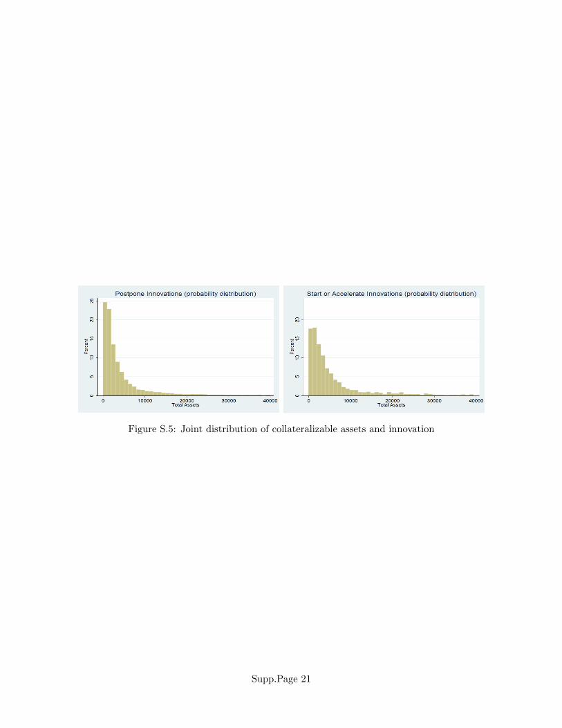
Figure S.5: Joint distribution of collateralizable assets and innovation

Supp.Page 21