credit risk management and jump models
TRANSCRIPT

Alma Mater Studiorum · Universita di Bologna
DOTTORATO DI RICERCA IN MATEMATICA
CICLO XXXI
Credit Risk Management and JumpModels
Presentata da: Sidy Diop
Coordinatore dottorato:Chiar.ma Prof.ssaGiovanna Citti
Supervisore:Chiar.mo Prof.Andrea Pascucci
Co-supervisore:Chiar.mo Dr.Marco Di Francesco
Esame finale 2018

Abstract
Since the breakout of global financial crisis 2007-2009 and the failures of system-relevant
financial institutions such as Lehman Brothers, Bear Stearns and AIG, improving credit risk
management models and methods is among the top priorities for institutional investors. Indeed,
the effectiveness of the traditional quantitative models and methods have been reduced by
the new complex credit derivatives introduced by the the financial innovations. The level of
implication of the credit default swaps (CDSs) in the crisis makes the CDS market an interesting
and active field of research. This doctoral thesis comprises three research papers that seek
to improve and create corporate and sovereign credit risk models, to provide an approximate
analytic expressions for CDS spreads and a numerical method for partial differential equation
arisen from pricing defaultable coupon bond.
First, an extension of Jump to Default Constant Elasticity Variance in more general and
realistic framework is provided (see Chapter 3). We incorporate, in the model introduced in [9],
a stochastic interest rate with possible negative values. In addition we provide an asymptotic
approximation formula for CDS spreads based on perturbation theory. The robustness and
efficiency of the method is confirmed by several calibration tests on real market data.
Next, under the model introduced in Chapter 3, we present in Chapter 4 a new numerical
method for pricing non callable defaultable bond. we propose appropriate numerical schemes
based on a Crank-Nicolson semi-Lagrangian method for time discretization combined with
biquadratic Lagrange finite elements for space discretization. Once the numerical solutions
of the PDEs are obtained, a post-processing procedure is carried out in order to achieve the
value of the bond. This post-processing includes the computation of an integral term which
is approximated by using the composite trapezoidal rule. Finally, we present some numerical
results for real market bonds issued by different firms in order to illustrate the proper behaviour
of the numerical schemes.
Finally, we introduce a hybrid Sovereign credit risk model in which the intensity of default of a
sovereign is based on the jump to default extended CEV model (see Chapter 5). The model

captures the interrelationship between creditworthiness of a sovereign, its intensity to default
and the correlation with the exchange rate between the bond’s currency and the currency
in which the CDS spread are quoted. We consider the Sovereign Credit Default Swaps Italy,
during and after the financial crisis, as a case of study to show the effectiveness of our model.

Acknowledgements
First and foremost, I would like to express my sincere gratitude to my supervisor, Professor
Andrea Pascucci for his great support of my doctoral studies and the many valuable comments
and discussions. Without his assistance and inspiration, the work in this dissertation would not
be possible.
I thank Dr. Marco Di Francesco very much for co-supervising my doctoral thesis and adding to
it with his thoughtful comments and suggestions. His guidance helped me in all the time of
research and writing of this thesis.
My sincere thanks also goes to Professor Carlos Vazquez, and Dr. Marıa Del Carmen, from the
University of A Coruna, who provided me an opportunity to join their team, and who gave
access to the laboratory and research facilities . Without their precious support it would not
be possible to conduct this research.
I thank my colleagues at UnipolSai who created a collaborative and stimulating working
environment, notably Martina, Lorenzo, Elisa, Festino and Gian Luca De Marchi for his
collaboration. Also I thank my friends in the Mathematics Department of the University of
Bologna.
Last but not the least, I would like to thank my family: my parents and my brothers and sisters
for supporting me spiritually throughout writing this thesis and my life in general.


To my beloved parents for their love, endless support and sacrifices.


Contents
Abstract c
Acknowledgments e
1 Introduction 1
2 Preliminaries 7
2.1 Default Times with Stochastic Intensity . . . . . . . . . . . . . . . . . . . . . . 7
2.1.1 Default time . . . . . . . . . . . . . . . . . . . . . . . . . . . . . . . . . 7
2.1.2 Conditional expectation with respect to Ft . . . . . . . . . . . . . . . . 8
2.1.3 Enlargements of Filtrations . . . . . . . . . . . . . . . . . . . . . . . . . 8
2.1.4 Conditional expectation with respect to Gt . . . . . . . . . . . . . . . . 10
2.1.5 Conditional survival probability . . . . . . . . . . . . . . . . . . . . . . . 13
2.2 Equivalent Probabilities, Radon-Nikodym Densities and Girsanov’s Theorem . 14
2.2.1 Decomposition of PMartingales as Qsemi-martingales . . . . . . . . . . 16
2.2.2 Girsanov’s Theorem . . . . . . . . . . . . . . . . . . . . . . . . . . . . . 16
i

j CONTENTS
2.2.3 Risk-neutral measure . . . . . . . . . . . . . . . . . . . . . . . . . . . . . 18
2.3 PDE approach for pricing defaultable contingent claim . . . . . . . . . . . . . . 19
3 CDS calibration under an extended JDCEV model 23
3.1 Introduction . . . . . . . . . . . . . . . . . . . . . . . . . . . . . . . . . . . . . . 23
3.2 CDS spread and default probability . . . . . . . . . . . . . . . . . . . . . . . . . 24
3.2.1 Valuation of CDS . . . . . . . . . . . . . . . . . . . . . . . . . . . . . . . 26
3.2.2 Market CDS Spread . . . . . . . . . . . . . . . . . . . . . . . . . . . . . 27
3.3 CDS spread approximation under extended JDCEV model . . . . . . . . . . . . 29
3.4 CDS calibration and numerical tests . . . . . . . . . . . . . . . . . . . . . . . . 36
3.4.1 CDS calibration . . . . . . . . . . . . . . . . . . . . . . . . . . . . . . . 37
4 Numerical method for evalution of a defaultable coupond bond 45
4.1 Introduction . . . . . . . . . . . . . . . . . . . . . . . . . . . . . . . . . . . . . . 45
4.2 Model and PDE formulation for price of defaultable bond . . . . . . . . . . . . 46
4.3 Numerical methods for picing defaultable bond . . . . . . . . . . . . . . . . . . 49
4.3.1 Localization procedure and formulation in a bounded domain . . . . . . 49
4.3.2 Time discretization . . . . . . . . . . . . . . . . . . . . . . . . . . . . . . 53
4.3.3 Finite elements discretization . . . . . . . . . . . . . . . . . . . . . . . . 55
4.3.4 Composite trapezoidal rule . . . . . . . . . . . . . . . . . . . . . . . . . 56
4.4 Empirical Results . . . . . . . . . . . . . . . . . . . . . . . . . . . . . . . . . . 56

4.4.1 Example 1 . . . . . . . . . . . . . . . . . . . . . . . . . . . . . . . . . . . 57
4.4.2 Example 2 . . . . . . . . . . . . . . . . . . . . . . . . . . . . . . . . . . . 58
5 Sovereign CDS calibration under a hybrid Sovereign Risk Model 63
5.1 Introduction . . . . . . . . . . . . . . . . . . . . . . . . . . . . . . . . . . . . . . 63
5.2 Model and Set-up . . . . . . . . . . . . . . . . . . . . . . . . . . . . . . . . . . . 69
5.3 Sovereign Credit Default Swap spread . . . . . . . . . . . . . . . . . . . . . . . 75
5.4 Sovereign CDS calibration and empirical test . . . . . . . . . . . . . . . . . . . 83
6 Conclusion 89
7 Appendix 95
7.1 Appendix A: Asymptotic approximation for solution to Cauchy problem . . . . 95
7.2 Appendix B: Further calibration tests I . . . . . . . . . . . . . . . . . . . . . . 105
7.3 Appendix C: Further calibration tests II . . . . . . . . . . . . . . . . . . . . . . 109
Bibliography 113
k

l

List of Tables
3.1 Calibration to ZCB. . . . . . . . . . . . . . . . . . . . . . . . . . . . . . . . . . 37
3.2 Calibration to UBS AG CDS spreads (uncorrelated case). . . . . . . . . . . . . 39
3.3 Calibration to UBS AG CDS spreads (Correlated case). . . . . . . . . . . . . . 39
3.4 Calibration to BNP Paribas CDS spreads (uncorrelated case). . . . . . . . . . . 40
3.5 Calibration to BNP CDS spreads (Correlated case). . . . . . . . . . . . . . . . 40
3.6 Computational Times . . . . . . . . . . . . . . . . . . . . . . . . . . . . . . . . 41
3.7 Risk-neutral UBS AG survival probabilities (uncorrelated case). . . . . . . . . . 41
3.8 Risk-neutral UBS AG survival probabilities (correlated case). . . . . . . . . . . 41
3.9 Risk-neutral BNP Paribas survival probabilities (uncorrelated case). . . . . . . 42
3.10 Risk-neutral BNP Paribas survival probabilities (correlated case). . . . . . . . . 42
3.11 Impact of the correlation . . . . . . . . . . . . . . . . . . . . . . . . . . . . . . . 44
4.1 Different finite element meshes (number of elements and nodes). . . . . . . . . 57
4.2 Parameters of the model for the UBS bond. . . . . . . . . . . . . . . . . . . . . 58
4.3 Market and model values of the ZCB. . . . . . . . . . . . . . . . . . . . . . . . 58
m

4.4 Value of the UBS bond for different meshes and time steps. . . . . . . . . . . . 60
4.5 Parameters of the model for the JP Morgan bond. . . . . . . . . . . . . . . . . 60
4.6 Value of the JP Morgan bond for different meshes and time steps. . . . . . . . 60
4.7 New method vs Monte Carlo simulation . . . . . . . . . . . . . . . . . . . . . . 61
5.1 Calibration to Italy USD CDS quoted as COB November, 15th, 2011 . . . . . . 84
5.2 Calibration to Italy USD CDS quoted as COB May, 30th 2017 . . . . . . . . . 85
7.1 Calibration to Caixa Bank SA CDS spreads (Correlated case). . . . . . . . . . 106
7.2 Calibration to Citigroup Inc CDS spreads (Correlated case). . . . . . . . . . . . 106
7.3 Calibration to Commerzbank AG CDS spreads (Correlated case). . . . . . . . . 107
7.4 Calibration to Mediobanca SpA spreads (Correlated case). . . . . . . . . . . . . 107
7.5 Calibration to Deutsche Bank AG spreads (Correlated case). . . . . . . . . . . 108
7.6 Calibration to France USD CDS quoted as COB November, 15th, 2011. . . . . 109
7.7 Calibration to France USD CDS quoted as COB May, 30th 2017. . . . . . . . . 110
7.8 Calibration to Portugal USD CDS quoted as COB November, 15th, 2011. . . . 110
7.9 Calibration to Portugal USD CDS quoted as COB May, 30th 2017. . . . . . . . 111
7.10 Calibration to Spain USD CDS quoted as COB November, 15th, 2011. . . . . . 111
7.11 Calibration to Spain USD CDS quoted as COB May, 30th 2017. . . . . . . . . 112
n

List of Figures
3.1 CDS Spreads with fixed maturity . . . . . . . . . . . . . . . . . . . . . . . . . . 26
3.2 Dependence of the error on the maturity . . . . . . . . . . . . . . . . . . . . . . 42
4.1 Value of the UBS bond . . . . . . . . . . . . . . . . . . . . . . . . . . . . . . . . 61
4.2 Value of the JP Morgan bond . . . . . . . . . . . . . . . . . . . . . . . . . . . . 61
5.1 Government Bonds Spread versus Bund . . . . . . . . . . . . . . . . . . . . . . 65
5.2 SCDS foreign Survival Probabilities of Italy USD CDS quoted as COB November,
15th, 2011 . . . . . . . . . . . . . . . . . . . . . . . . . . . . . . . . . . . . . . . 87
5.3 SCDS foreign Survival Probabilities of Italy USD CDS quoted as COB May,
30th 2017 . . . . . . . . . . . . . . . . . . . . . . . . . . . . . . . . . . . . . . . 87
7.1 Dependence of the error on the maturity . . . . . . . . . . . . . . . . . . . . . . 109
o

p

Chapter 1
Introduction
‘All of life is the management of risk, not its elimination.’
Walter Wriston, former chairman of Citicorp
Credit risk is most simply defined as the potential loss in the mark-to-market value that
may be incurred due to the occurrence of a credit event. A credit event is any sudden and
perceptible change in the counterparty’s ability to perform its obligations: Bankruptcy, failure
to pay, restructuring, repudiation, moratorium, obligation, acceleration and obligation default.
Credit default also includes sovereign risk. This happens , for instance, when countries impose
foreign-exchange controls that make it impossible for counterparties to respect the terms of a
contract. Credit risk management is described in the financial literature as being concerned
with identifying and managing a firm’s exposure to credit risk.
The financial innovations, after the decision of the US Federal Reserve to lower the interest
rate to 1%, followed by the housing bubble, have introduced new complex instruments in the
1

2 Chapter 1. Introduction
financial market. This led to a rapid growth in the market for credit derivatives, which has
become the third-largest derivatives market, after interest rate and foreign exchange derivatives,
in terms of gross market value, accounting for USD 1.2 quadrillion as of June 2018. Among
the credit derivatives, the credit default swaps (CDS) are the most popular and influential
in trading credit risk. However, their level of implication in the recent financial scandals is
significant: in the sub-prime crisis in 2007-2008 or the trading losses by the “London Whale”
at JP Morgan Chase in 2012. Most of the new credit derivatives have limited historical data
and required assumptions regarding risk and correlations with other instruments, reducing the
effectiveness and robustness of quantitative risk models prior to the crisis. To deal with these
complex financial instruments, the ”traditional” models either omitted them and waited until
they obtained enough historical data, or created simple approximations or just used proxies. It
followed failures of credit risk management. Then, improving models and methods is among
the top priorities for institutional investors in the wake up of the recent global financial.
Nowadays the credit risk models can be divided into two primary classes of credit risk modeling
approach: the structural approach and the reduced form approach also known as intensity form
approach. Structural models, first developed by Black, Scholes and Merton, employ modern
option pricing theory in corporate debt valuation. In 1974, Robert Merton, in [34], proposed
the first structural model for assessing credit risk of a company by building the company’s
equity as a call option on its asset, thus allowing the Black-Scholes option pricing method.
The structural model has known many improvements due to the simplicity and the several
assumptions of its initial version in [34]. Black and Cox [4] introduced the first extension by
considering a possible default event before maturity and assumed that default can also occur at
the first time the asset price goes below a fixed value. Geske [15] included a coupon bond in
the model. Ramaswamy and Sundaresan [40] as well as Kim [25] considered a default event at
coupon payment dates and incorporated a stochastic interest rate following a CIR model. In
1995 Longstaff and Schwartz [28] extended the model by assuming that default can happen at

3
anytime, while Zhou [41] modeled the value of the firm as a jump-diffusion process.
The reduced-form models, on the other hand, trace their roots back to the work of Jarrow
and Turnbull [17] and subsequently studied by Jarrow and Turnbull [18], Duffie and Singleton
[11], and Madan and Unal [31], among others. In reduced form approach models, the set of
information requires less detailed knowledge about the firm’s assets and liabilities than the
structural approach. They are consistent with available market information. The idea is to
observe the filtration generated by the default time and the vector of state variables , where the
default time is a stopping time generated by a Cox process with an intensity process depending
on the state variables which follows a diffusion process. We call the payoff to the firm’s debt in
the event of default by recovery rate, given by a stochastic process. In 2006, Carr and Linetsky
introduced the Jump to Default Constant Elasticity Volatility model [9], an improvement of a
reduced approach, which unifies credit and equity models into the framework of deterministic
and positive interest rates. Assuming that the stock price follows a diffusion process with a
possible jump to zero, hazard rate of default is an increasing affine function of the instantaneous
variance of returns on the stock price, and stock volatility is defined as in the Constant Elasticity
of Variance (CEV) model, the authors developed a model that captures the following three
observations:
credit default swap (CDS) spreads and corporate bond yields are both positively related
to implied volatilities of equity options;
realized volatility of stock is negatively related to its price level;
equity implied volatilities tend to be decreasing convex functions of option’s strike price.
The JDCEV model, thanks to the standard Bessel process with killing, provides an explicit
analytical expression for survival probabilities and CDS spreads. However, this approach
does not work in the case of a stochastic or negative interest rate. The main purpose of this

4 Chapter 1. Introduction
dissertation is, therefore, to extend the JDCEV models to a more general framework and to
provide approximate analytic expressions for CDS spreads for both corporate and sovereign.
In the second chapter, we summarize some preliminaries of mathematical theory (e.g. Ito
calculus, Girsanov’s theorem etc.) often used in the valuation of options (and other derivatives).
In the third chapter, we propose a new methodology for the calibration of a hybrid credit-equity
model to credit default swap (CDS) spreads and survival probabilities. We consider an extended
Jump to Default Constant Elasticity of Variance model incorporating stochastic and possibly
negative interest rates. Our approach is based on a perturbation technique that provides an
explicit asymptotic expansion of the credit default swap spreads. The robustness and efficiency
of the method is confirmed by several calibration tests on real market data.
In the fourth chapter, we consider the numerical solution of a two factor-model for the valuation
of defaultable bonds which pay coupons at certain given dates. We consider the extended
JDCEV model introduced in the previous chapter. From the mathematical point of view, the
valuation problem requires the numerical solution of two partial differential equations (PDEs)
problems for each coupon and with maturity those coupon payment dates. In order to solve
these PDE problems, we propose appropriate numerical schemes based on a Crank-Nicolson
semi-Lagrangian method for time discretization combined with biquadratic Lagrange finite
elements for space discretization. Once the numerical solutions of the PDEs are obtained,
a kind of post-processing is carried out in order to determine the value of the bond. This
post-processing includes the computation of an integral term which is approximated by using
the composite trapezoidal rule. Finally, we present some numerical results for real market bonds
issued by different firms in order to illustrate the proper behavior of the numerical schemes.
The fifth chapter presents a hybrid sovereign risk model in which the intensity of default of the
sovereign is based on the jump to default extended CEV model with a deterministic interest
rate. The model captures the interrelationship between creditworthiness of a sovereign, its

5
intensity to default and the correlation with the exchange rate between the bond’s currency
and the currency in which the CDS spread are quoted. We analyze the differences between the
default intensity under the domestic and foreign measure and we compute the default-survival
probabilities in the bond’s currency measure. We also give an approximation formula to
sovereign CDS spread obtained by using the same technique as in the Chapter 3. Finally, we
test the model on real market data by several calibration experiments to confirm the robustness
of our method.
We conclude the thesis and present,in the first section of the appendix, the theory of the
asymptotic approximation method used in third and fifth fourth chapters, and introduced in
[29]. The second and third sections in the appendix consist of results from calibration tests on
corporates and sovereigns credit default swap spreads.

6 Chapter 1. Introduction

Chapter 2
Preliminaries
In this chapter, we summarize some definitions and results from finance, stochastic calculus and
the theory of partial differential equations. We mainly focus on the risk-neutral measure and
Girsanov’s Theorem, enlargement filtrations and the PDE approach for pricing. The following
definitions and results are in major adapted from [21], [39] and [6]. More detailed information
can be found in these books.
2.1 Default Times with Stochastic Intensity
2.1.1 Default time
Let (Ω,G,P) be a probability space endowed with a filtration F and let λ be a positive F-adapted
process. We assume that there exists, on the space (Ω,G,P), a random variable Θ, independent
of F∞, with exponential law of parameter 1: P (Θ ≤ t) = e−t. We define the default time τ as
the first time when the increasing process Λt =∫ t
0 λsds exceeds the random level Θ, i.e.,
τ = inf t ≥ 0: Λt ≥ Θ.
7

8 Chapter 2. Preliminaries
In particular, τ ≥ s = Λs ≤ Θ. We assume that Λt <∞, ∀ t, and Λ∞ =∞.
2.1.2 Conditional expectation with respect to Ft
Lemma 2.1.1. The conditional distribution function of τ given the filtration σ−algebra Ft is,
for t ≥ s,
P (τ > s|Ft) = exp (−Λs).
Proof. The proof comes straightforward from the equality τ > s, the independence assumption
and the Ft-measurablity of Λs for s ≤ t
P (τ > s|Ft) = P (Λs < Θ|Ft) = exp (−Λs).
Remark 2.1.2. 1. for t < s, we obtain P (τ > s|Ft) = E (exp (−Λs|Ft)).
2. If the process λ is not positive, the process Λ is not increasing and we obtain, for s < t,
P (τ > s|Ft) = P
(supu≤s
Λu < Θ
)= exp
(− supu≤s
Λu
).
2.1.3 Enlargements of Filtrations
The problems of enlargement and immersion of filtration have been first introduced by K. Ito
[16] and then later studied in the seventies by Barlow [1], Jeulin and Yor [22]. Let F and G be
two filtrations. G is larger than F does not imply that a F-martingale is a G-martingale.
Definition 2.1.3 ((H) hypothesis). The filtration F is said to be immersed in G if any square
2.1. Default Times with Stochastic Intensity 9
integrable F-martingale is a G-martingale. That is
P (τ ≤ t|Ft) = P (τ ≤ t|F∞) = P (τ ≤ t|Fs) , ∀ t, s, t ≤ s.
Proposition 2.1.4. Hypothesis (H) is equivalent to any of the following properties:
(i) ∀ t ≥ 0, the σ-fields F∞ and Gt are conditionally independent given Ft
(ii) ∀ t ≥ 0, ∀At ∈ L1 (Gt) E (At|F∞) = E (At|Ft)
(iii) ∀ t ≥ 0, ∀F ∈ L1 (F∞) , E (F |Gt) = E (F |Ft).
In particular (H) holds if and only if every F−local martingale is G−local martingale.
Proof. For the proof, the reader can refer to the chapter 5 in [20].
Consider the default process Dt = 1τ≤t and Dt = σ (Ds : s ≤ t). We set the filtration
Gt = Ft ∨Dt, that is, the enlarged filtration generated by the underlying filtration F and the
default time process D. We write G = F∨D, the smallest filtration which contains the filtration
F and such that the default time τ is a G-stopping time. If At is an event in the σ-algebra Gt,
then there exists At ∈ Ft such that
At ∩ τ > t = At ∩ τ > t,
It follows that, if (Yt)t≥0 is a G-adapted process, there exists an F-adapted process (Yt)t≥0 such
that
Yt1t<τ = Yt1t<τ.

10 Chapter 2. Preliminaries
2.1.4 Conditional expectation with respect to Gt
Lemma 2.1.5. Let Y be an integrable random variable. Then
1τ>tE (Y |Gt) = 1τ>tE(Y 1τ>t|Ft
)E(1τ>t|Ft
) = 1τ>teΛtE
(Y 1τ>t|Ft
).
Proof. We have, by definition of the conditional expectation, that Yt = E (Y |Gt) is Gt-measurable.
Then
1τ>tYt = 1τ>tE (Y |Gt)
⇒ E(1τ>tYt|Ft
)= E
(1τ>tE (Y |Gt) |Ft
)⇒ YtE
(1τ>t|Ft
)= E
(1Y τ>t|Ft
)⇒ 1τ>tYt = 1τ>t
E(1Y τ>t|Ft
)E(1τ>t|Ft
) = 1τ>teΛtE
(Y 1τ>t|Ft
),
where the last equality comes from the lemma 2.1.1.
We denote by F the right-continuous cumulative distribution function of the random variable τ
defined as Ft = P(τ ≤ t) and we assume that Ft < 1 for any t ≤ T , where T is a finite horizon.
Corollary 2.1.6. If X is an integrable FT -measurable random variable, for t < T
E(X1T<τ|Gt
)= 1τ>te
ΛtE(Xe−ΛT |Ft
).
Proof. Since E(X1T<τ|Gt
)is equal to zero on the Gt-measurable set τ < t, then
E(X1T<τ|Gt
)= 1τ>tE
(X1T<τ|Gt
),
= 1τ>teΛtE
(X1T<τ1τ>t|Ft
), by lemma 2.1.5
= 1τ>teΛtE
(E(X1T<τ|FT
)|Ft),
2.1. Default Times with Stochastic Intensity 11
= 1τ>teΛtE
(XE
(1T<τ|FT
)|Ft),
= 1τ>teΛtE
(Xe−ΛT |Ft
).
Lemma 2.1.7. (i) Let h be a (bounded) F-predictable process. Then
E (hτ |Ft) = E
(∫ ∞0
huλue−Λudu|Ft
)= E
(∫ ∞0
hudFu|Ft)
and
E (hτ |Gt) = eΛtE
(∫ ∞t
huλudFu|Ft)1τ>t + hτ1τ≤t. (2.1.1)
In particular
E (hτ ) = E
(∫ ∞0
huλue−Λudu
)= E
(∫ ∞0
hudFu
).
(ii) The process (Dt −∫ t∧τ
0 λsds, t ≥ 0) is a G- martingale.
Proof. Let Bv ∈ Fv and h the elementary F-predictable process defined as ht = 1t>vBv.
Then,
E (hτ |Ft) = E(1τ>vBv|Ft
)= E
(E(1τ>vBv|F∞
)|Ft)
= E (BvP (τ > v|F∞) |Ft) = E(Bve
−Λv |Ft).
It follows that
E (hτ |Ft) = E
(Bv
∫ ∞v
λue−Λudu|Ft
)= E
(Bv
∫ ∞0
huλue−Λudu|Ft
)
and (i) is derived from the monotone class theorem. Equality (2.1.1) follows from the Lemma

12 Chapter 2. Preliminaries
2.1.5.
The martingale property (ii) follows from the integration by parts formula. Indeed, let s < t.
Then, on the one hand from the Lemma 2.1.5
E (Dt −Ds|Gs) = P (s < τ ≤ t|Gt) = 1s<τP (s < τ ≤ t|Fs)P (s < τ |Fs)
= 1s<τ(1− eΛsE
(e−Λt |Fs
)).
On the other hand, from part (i), for s < t,
E
(∫ t∧τ
s∧τλudu|Gs
)= E (Λt∧τ − Λs∧τ |Gs) = E (ψτ |Gt)
= 1s<τeΛsE
(∫ ∞s
ψuλue−Λudu|Fs
)
where ψu = Λt∧u − Λs∧u = 1s<u(Λt∧u − Λs). Consequently,
∫ ∞s
ψuλue−Λudu =
∫ t
s(Λu − Λs)λue
−Λudu+ (Λt − Λs)
∫ ∞t
λue−Λudu
=
∫ t
sΛuλue
−Λudu− Λs
∫ ∞s
λue−Λudu+ Λte
−Λt
=
∫ t
sΛuλue
−Λudu− Λse−Λs + Λte
−Λt
= e−Λs − e−Λt .
It follows that
E (Dt −Ds|Gs) = E
(∫ t∧τ
s∧τλydu|Gs
),
hence the martingale property of the process Dt −∫ t∧τ
0 λudu.

2.1. Default Times with Stochastic Intensity 13
2.1.5 Conditional survival probability
Let G be the survival hazard process, Gt := P(τ > t|Ft) = 1 − Ft. Since the default time is
constructed with a Cox process model, we can see that
Gt = E(1τ>t|Ft
)= exp
(−∫ t
0λudu
).
It follows that the immersion property holds.
Lemma 2.1.8. Let X be an FT -measurable integrable random variable. Then, for t < T ,
E(X1T<τ|Gt
)= 1τ>t (Gt)
−1E (XGT |Ft) .
Proof. The proof is the same as in Corollary 2.1.6. Indeed
1τ>tE(X1T<tτ|Gt
)= 1τ>txt,
where xt is Ft-measurable. Taking conditional expectations w.r.t Ft of both sides, we deduce
xt =E(X1τ>T|Ft
)E(1τ>t|Ft
) = 1τ (Gt)−1E (XGT |Ft) .
Lemma 2.1.9. Let h be an F-predictable process. Then
E(hτ1τ≤T|Gt
)= hτ1τ≤t − 1τ>t (G)−1
E
(∫ T
thudGu|Ft
)
Proof. The proof follows the same line as that of Lemma 2.1.7.

14 Chapter 2. Preliminaries
2.2 Equivalent Probabilities, Radon-Nikodym Densities and
Girsanov’s Theorem
Let P and Q be two probabilities defined on the same measurable space (Ω,F). The probability
Q is said to be absolutely continuous with respect to P, (denoted Q P) if P = 0 implies
Q (A) = 0, for any A ∈ F. In that case, there exists a positive, F-measurable random variable
L, called the Radon-Nikodym density of Q with respect to P, such that
∀A ∈ F, Q (A) = EP (L1A) .
This random variable L satisfies EP (L) = 1 and for any Q-integrable random variable X,
EQ (X) = EP (XL). The notationdQ
dP= L ( or Q|F = LP|F) is common use, in particular in
the chain of equalities
EQ (X) =
∫XdQ =
∫X
dQ
dPdP =
∫XLdP = EP (XL) .
The probabilities P and Q are said to be equivalent, (this will be denoted P ∼ Q), if they
have the same null sets, i.e., if for any A ∈ F,
Q (A) = 0 ⇐⇒ P (A) = 0,
or equivalently, if Q P and P Q. In that case, there exists a strictly positive, F-
measurable random variable L, such that Q (A) = EP (L1A). Note that dPdQ = L−1 and
P (A) = EQ(L−11A
).
Conversely, if L is a strictly positive F-measurable r.v., with expectation 1 under P, then
Q = L·P defines a probability measure on F, equivalent to P. From the definition of equivalence,
if a property holds almost surely (a.s.) with respect to P, it also holds a.s. for any probability

2.2. Equivalent Probabilities, Radon-Nikodym Densities and Girsanov’s Theorem 15
Q equivalent to P. Two probabilities P and Q on the same probability space (Ω,F) are said to
be equivalent if they have the same negligible sets on Ft, for every t ≥ 0, i.e. ,if Q|Ft ∼ P|Ft .
In that case, there exists a strictly positive F-adapted process (Lt)t≥0 such that Q|Ft = LtP|Ft .
Furthermore, if τ is a stopping time , then
Q|Fτ∩τ<∞ = Lτ · P|Fτ∩τ<∞.
Proposition 2.2.1. (Bayes Formula) Suppose that Q and P are equivalent on FT with Radon-
Nikodym density L. Let X be a Q-integrable FT -measurable random variable, then, for t < T
EQ (X|Ft) =EP (LTX|Ft)
Lt.
Proof. The proof follows immediately from the definition of conditional expectation. To check
that Ft-measurable r.v. Z = EP(LTX|Ft)Lt
is the Q-conditional expectation of X, we prove that
EQ (FtX) = EQ (FtZt) for any bounded Ft-measurable r.v. Ft. This follows from the equalities
EQ (FtX) = EP (LTFtX) = EP (FtEP (XLT |Ft))
= EQ(FtL
−1t EP (XLT |Ft)
)= EQ (FtZ) .
Proposition 2.2.2. Let Q and P be two locally equivalent probability measures with Radon-
Nikodym density L. A process M is a Q-martingale if and only if a process LM is a P-martingale.
By localization, this result remains true for local martingales.
Proof. Let M be a Q-martingale. From the Bayes formula, we obtain, for s ≤ t,
Ms = EQ (Mt|Fs) =EP (LtMt|Fs)
Ls

16 Chapter 2. Preliminaries
and the result follows. The converse part is now obvious.
2.2.1 Decomposition of PMartingales as Qsemi-martingales
Theorem 2.2.3. Let Q and P be two locally equivalent probability measures with Radon-
Nikodym density L. We assume that the process L is continuous. If M is a continuous P-local
martingale, then the process M defined by
dM = dM − 1
Ld〈M,L〉
is a continuous Q-local martingale. If N is another continuous P-local martingale,
〈M,N〉 = 〈M, N〉 = 〈M, N〉.
Proof. From Proposition 2.2.2, it is enough to check that ML is a P-local martingale, which
follows easily from Ito’s calculus.
Corollary 2.2.4. Under the hypothesis of Theorem 2.2.3, we may write the process L as
a Doleans-Dade martingale: Lt = E (ξ)t, where ξ is an F-local martingale. The process
M = M − 〈M, ξ〉 is a Q-local martingale.
2.2.2 Girsanov’s Theorem
Assume that F is generated by a Brownian motion W and let L be the Radon-Nikodym density
of the locally equivalent measures P and Q. Then the martingale L admits a representation of
the form dLt = ψtdWt. Since L is strictly positive, this equality takes the form dLt = −θtLtdWt.
where θ = −ψL . It follows that
Lt = exp
(−∫ t
0θsdWs −
1
2
∫ t
0θ2sds
)= E (ξ)t ,

2.2. Equivalent Probabilities, Radon-Nikodym Densities and Girsanov’s Theorem 17
where ξt = −∫ t
0 θsdWs.
Proposition 2.2.5. Let W be an (P,F)-Brownian motion and let θ be an F-adapted process
such that the solution of the stochastic differential equation (SDE)
dLT = −LtθtdWt, L0 = 1
is a martingale. We set Q|Ft = LtP|Ft. Then the process W admits a Q-semi-martingale
decomposition W as Wt = Wt −∫ t
0 θsds where W is a Q-Brownian motion.
Proof. From dLt = −LtθtdWt, using the Girsanov’s theorem 2.2.3, we obtain that the decompo-
sition of W under Q is Wt −∫ t
0 θsds. The process W is a Q-semi-martingale and its martingale
part W is a Brownian motion. This last fact follows from Levy’s theorem, since the bracket of
W does not depend on the (equivalent) probability.
Remark 2.2.6. (Multidimensional case) Let W be an n-dimensional Brownian motion and θ be
an n-dimensional adapted process such that∫ t
0 ||θs||2ds <∞, a.s.. Define the local martingale
L as the solution of
dLt = Ltθt · dWt = Lt
(n∑i=1
θitdWit
),
so that
Lt = exp
(∫ t
0θs · dWs −
1
2
∫ t
0||θs||2ds
).
If L is a martingale, the n-dimensional process(Wt = Wt −
∫ t0 θsds, t ≥ 0
)is a Q-martingale,
where Q is defined by Q|Ft = LtP|Ft . Then W is an n-dimensional Brownian motion (and in
particular its components are independent).
If W is a Brownian motion with correlation matrix Λ, then, since the brackets do not depend

18 Chapter 2. Preliminaries
on the probability, under Q, the process
Wt = Wt −∫ t
0θs · Λds
is a correlated Brownian motion with the same correlation n matrix Λ.
2.2.3 Risk-neutral measure
The value of a derivative can be calculated as the expectation of the derivative payoff over all
possible asset price paths which affect the payoff. The measure under which this expectation is
taken is critical, determining whether the pricing of derivatives is in line with the standard
no-arbitrage assumptions present in almost all models of derivative pricing. The fundamental
theorem of asset pricing tells us that a complete market is arbitrage free if and only if there
exists at least one risk-neutral probability measure. Under this measure all assets have an
expected return which is equal to the risk-free rate.
The history of the development of risk-neutral pricing is one that spans decades and largely
follows the development of quantitative finance. Consider the standard assumption that there
is a stock whose price satisfies
dSt = µtStdt+ σtStdWt.
In addition, suppose that we have an adapted interest rate process rt, t ≥ 0. The corresponding
discount process follows
dDt = −rtDtdt.
The discounted stock price process is given by
d (DtSt) = rtDtSt (θdt+ dWt) ,

2.3. PDE approach for pricing defaultable contingent claim 19
where we define the market price of risk to be
θt =αt − rtσt
.
We introduce a probability measure Q defined in Girsanov’s theorem, which uses the market
price of risk θt. In terms of Brownian motion W , we rewrite the discount stock price as
d (DtSt) = σtDtStdWt
We call Q the risk-neutral measure.
2.3 PDE approach for pricing defaultable contingent claim
We assume that P represents the real-world probability as opposed to the risk neutral probability
measure denoted by Q and chosen by the market. We assume that a defaultable risky asset S
and a stochastic interest rate r are the only assets available in the market whose risk-neutral
dynamics are as follows:
dSt = µ (St, rt) dt+ σ (St, rt) dW 1
t
drt = α (St, rt) dt+ β (St, rt) dW 2t
dW 1t dW 2
t = ρdt.
The filtration F represents the quantity of information on the assets and the filtration D is
generated by τ which models the time to default of the defaultable asset. We assume that
the market is complete and arbitrage-free. Consider a contingent claim H on the defaultable
risky asset S that consists of a payment of an amount H = h (ST , rT ) at maturity if no default
occurs prior to maturity T . The time-t price V (t,H) of the contingent claim is given, from

20 Chapter 2. Preliminaries
Corollary 2.1.6, by
V (t,H) = E(e−∫ Tt (ru+λu)duh (ST , rT ) |Ft
).
Let
f (t, St, rt) = V (t,H)
and
g (St, rt) = E(e−∫ T0 (ru+λu)duh (ST , rT ) |Ft
).
As soon as g is smooth enough (see [24]), Ito’s formula leads to
dg (St, rt) =
(∂tg (St, rt) + µ (St, rt) ∂Sg (St, rt) +
1
2σ (St, rt)
2 ∂2Sg (St, rt) + α (St, rt) ∂rg (St, rt)
+1
2β (St, rt)
2 ∂2rg (St, rt) + ρβ (St, rt)σ (St, rt) ∂Srg (St, rt)− (rt − λt) g (St, rt)
)dt
+ σ (St, rt) ∂Sg (St, rt) dW 1t + β (St, rt) ∂rg (St, rt) dW 2
t .
Since the process (g (St, rt) , t ≥ 0) is a martingale, the dt-term is equal to zero. That is
0 =∂tg (St, rt) + µ (St, rt) ∂Sg (St, rt) +1
2σ (St, rt)
2 ∂2Sg (St, rt)
+ ρβ (St, rt)σ (St, rt) ∂Srg (St, rt) + α (St, rt) ∂rg (St, rt) +1
2β (St, rt)
2 ∂2rg (St, rt)− (rt − λt) g (St, rt) ,
and
g (ST , rT ) = E(e−∫ TT (ru+λ−u)duh (ST ) |FT
)= h (ST ) .
Proposition 2.3.1. Let the risk-neutral dynamics of the defaultable risky asset and the stochas-

2.3. PDE approach for pricing defaultable contingent claim 21
tic interest rate be defined as
dSt = µ (St, rt) dt+ σ (St, rt) dW 1
t
drt = α (St, rt) dt+ β (St, rt) dW 2t
dW 1t dW 2
t = ρdt.
Assume that u solves the Cauchy problem
(∂t + A)u (t, S, r) = 0, t ∈ [0, T ), S ≥ 0, r ∈ R
u (T, S, r) = h (S, r) , S ≥ 0, r ∈ R,
with
A = ∂t + µ (St, rt) ∂S +1
2σ (St, rt)
2 ∂2S + α (St, rt) ∂r +
1
2β (St, rt)
2 ∂2r + ρβ (St, rt)σ (St, rt) ∂Sr − (rt − λt) .
Then the value at time t of the contingent claim H = h (ST , rT ) is equal to u (t, St, rt).

22 Chapter 2. Preliminaries
Chapter 3
CDS calibration under an extended
JDCEV model
3.1 Introduction
The purpose of this chapter is to provide a robust and efficient method to calibrate a hybrid
credit-equity model to the CDS market. Credit Default Swaps (CDS) are the most influential
and traded credit derivatives. They played an important role in the recent financial scandals:
in the sub-prime crisis in 2007-2008 or the trading losses by the “London Whale” at JP Morgan
Chase in 2012. On the other hand, large global banks have been successfully exploiting the CDS
market in their trading activities: for example, JP Morgan has several trillions of dollars of
CDS notional outstanding. In parallel, the academic research on CDS, liabilities and derivatives
in general has quickly expanded in the recent years. Among the most important contributions,
the Jump to Default Constant Elasticity of Variance (JDCEV) model by Carr and Linetsky
[9, 32, 33] is one of the first attempts to unify credit and equity models into the framework of
deterministic and positive interest rates. The authors of [9] claim that credit models should
23

24 Chapter 3. CDS calibration under an extended JDCEV model
not ignore information on stocks and there exists a connection among stock prices, volatilities
and default intensities. Indeed, earlier research on credit models (e.g. [10, 18, 19] was more
focused on how to palliate the absence of the bankruptcy possibility in classical option pricing
theory and take into account that in the real world firms have a positive probability of default
in finite time.
Nowadays the restrictive assumption of positive and deterministic interest rates of the JDCEV
model is not realistic and contradicts market observations. To incorporate stochastic and
possibly negative interest rates into the JDCEV model, we propose a fast and efficient technique
to compute CDS spreads and default probabilities for calibration purposes. In doing this we
employ a recent methodology introduced in [29, 37], which consists of an asymptotic expansion
of the solution to the pricing partial differential equation. Our method allows to calibrate
the extended JDCEV model to real market data in real time. To assess the robustness of the
approximation method and the capability of the model of reproducing price dynamics, we
provide several tests on UBS AG and BNP Paribas CDS spreads.
This chapeter is organized as follows. In Section 3.2 we set the notations and review the
jump to default diffusion model. In Section 3.3 we introduce an extended JDCEV model with
stochastic interest rates and provide explicit approximation formulas for the CDS spreads and
the risk-neutral survival probabilities. Section 3.4 contains the numerical tests: we consider
both the cases of correlated or uncorrelated spreads and interest rates; we calibrate the model to
market data of CDS spreads and compute the risk-neutral survival probabilities: a comparison
with standard Monte Carlo methods is provided as well.
3.2 CDS spread and default probability
We consider a probability space (Ω,G,Q) carrying a standard Brownian motion W and an
exponential random variable ε ∼ Exp(1) independent of W . We assume, for simplicity, a

3.2. CDS spread and default probability 25
frictionless market, no arbitrage and take an equivalent martingale measure Q as given. All
stochastic processes defined below live on this probability space and all expectations are taken
with respect to Q.
Let S be the pre-default stock price. We assume that the dynamics of X = log S are given by
dXt =
(rt − 1
2σ2 (t,Xt) + λ (t,Xt)
)dt+ σ (t,Xt) dW 1
t ,
drt = κ (θ − rt) dt+ δdW 2t ,
dW 1t dW 2
t = ρdt,
where the interest rate rt follows the Vasicek dynamics with parameters κ, θ, δ > 0. The
time- and state-dependent stock volatility σ = σ(t,X) and default intensity λ = λ(t,X)
are assumed to be differentiable with respect to X and uniformly bounded. In general the
price can become worthless in two scenarios: either the process eX hits zero via diffusion
or a jump-to-default occurs from a positive value. The default time ζ can be modeled as
ζ = ζ0 ∧ ζ, where ζ0 = inft > 0 | St = 0 is the first hitting time of zero for the stock price
and ζ = inft ≥ 0 | Λt ≥ ε is the jump-to-default time with intensity λ and hazard rate
Λt =∫ t
0 λ(s,Xs)ds. In what follows, we denote by F = Ft, t ≥ 0 the filtration generated
by the pre-default stock price and by D = Dt, t ≥ 0 the filtration generated by the process
Dt = 1ζ≤t. Eventually, G = Gt, t ≥ 0, Gt = Ft ∨Dt is the enlarged filtration.
A Credit Default Swap (CDS) is one of the most representative financial instruments depending
on default probabilities of firms. Designed to protect against default, a CDS with constant
rate R and recovery at default (1− η) is a contract between a party A (protection buyer), the
buyer of the protection against a reference entity C which defaults at time ξ, and a party B
(protection seller). Party A pays a premium R of the CDS notional amount N to the seller B
until ξ ∧ T at some predetermined date ti ≤ T with interval time α, where T is the maturity of
the CDS. If the default occurs prior to T , the seller pays, at the default time ξ, (1− η(ξ)) of N

26 Chapter 3. CDS calibration under an extended JDCEV model
to the buyer.
B → protection (1− η(ξ)) at ξ, default time of C, if ξ < T → A
B ← rate R at t1, t2, · · · , ξ ∧ T ← A
(1 − η) is called the loss-given-default, represents the default protection and R is the CDS
rate, also termed spread, premium or annuity of the CDS. Figure 3.1 represents the evolutions
of 5 years maturity CDS spreads of large corporates with respect to the observation date t
(t 7→ CDS(t, 5Y )).
Figure 3.1: CDS Spreads with fixed maturity
Evolution of 5 years CDS Spreads in function of observation date of four large corporates in the CDS market.
3.2.1 Valuation of CDS
Consider a CDS contract with rate R, default recovery (1 − η) and maturity time T . By
definition, its market value at time t is given by the expectation of the difference of the
discounted payoffs of the protection and premium legs
Vt (R) = EQ
(e−∫ ξt rudu (1− η (ξ))1ξ≤T −
M∑i=it
e−∫ tit ruduαR1ξ>ti|Gt
)(3.2.1)

3.2. CDS spread and default probability 27
where it = inf i ∈ 1, 2, · · · , M : t ≤ ti with tM = T .
Proposition 3.2.1. The price of a CDS at time t ∈ [0, T ] is given by
Vt (R) = 1t<ξ
(EQ(∫ T
te−∫ st (ru+λu)du (1− η (s))λsds|Ft
)−
M∑i=it
EQ(αRe−
∫ Tt (ru+λu)du|Ft
)).
Proof. The proof comes straightforward from Corollary 2.1.6 and Lemma 2.1.9 by setting
hs = (1− η (s)) e−∫ st rudu and Xi = e−
∫ tit rudu.
3.2.2 Market CDS Spread
Definition 3.2.2. A market CDS spread starting at t is a CDS initiated at time t whose value
is equal to zero . A T-maturity market CDS spread at time t is the level of the rate R = R(t, T )
that makes a T-maturity CDS starting at t valueless at its inception. A market CDS spread
at time t is thus determined by the equation Vt(R(t, T )) = 0, where V is defined by (3.2.1).
Hence, on 1t<ξ, we have
R (t, T ) =EQ(∫ T
t e−∫ st (ru+λu)du (1− η (s))λsds|Ft
)∑M
i=itEQ(αe−
∫ Tt (ru+λu)du|Ft
) . (3.2.2)
Proposition 3.2.3. Consider a CDS contract with constant default recovery (1− η), spread R
paid at premium payment dates ti, i = 1, 2, · · · M , so that that α = ti+1 − ti = TM . Then, at

28 Chapter 3. CDS calibration under an extended JDCEV model
time t = 0, the spread R := R (0, T ) is given by
R =(1− η)
(1− E
[e−∫ T0 (ru+λ(u,Xu))du
]−∫ T
0 E[e−∫ s0 (ru+λ(u,Xu))durs
]ds)
TM
M∑i=1E[e−∫ ti0 (ru+λ(u,Xu))du
] . (3.2.3)
Proof. From the definition of equation (3.2.2), the spread at time t = 0 is given by
R =(1− η)E
[∫ T0 e−
∫ s0 (ru+λ(u,Xu))duλ(s,Xs)ds
]TM
M∑i=1E[e−∫ ti0 (ru+λ(u,Xu))du
] . (3.2.4)
The statement follows by replacing the following identities in (3.2.4):
e−∫ s0 (ru+λ(u,Xu))duλ(s,Xs) = − ∂
∂s
(e−∫ s0 (ru+λ(u,Xu))du
)− rse−
∫ s0 (ru+λ(u,Xu))du,
and
∫ T
0e−∫ s0 (ru+λ(u,Xu))duλ(s,Xs)ds = 1−
(e−∫ T0 (ru+λ(u,Xu))du +
∫ T
0e−∫ s0 (ru+λ(u,Xu))dursds
).
Remark 3.2.4. The default intensity λ(t,Xt) can be considered as the instantaneous probability
that the stock will default between t and t+ dt, conditioned on the fact that no default has
happened before:
λ(t,Xt)dt = Q (t ≤ ζ < t+ dt | ζ ≥ t) .
The survival probability up to time t is defined as
Q (t) := E[e−∫ t0 λ(u,Xu)du
]. (3.2.5)

3.3. CDS spread approximation under extended JDCEV model 29
3.3 CDS spread approximation under extended JDCEV model
In the JDCEV model the stock volatility is of the form
σ(t,X) = a(t)e(β−1)X
where β < 1 and a(t) > 0 are the so-called elasticity parameter and scale function. The default
intensity is expressed as a function of the stock volatility and the stock log-price, as follows
λ(t,X) = b(t) + c σ(t,X)2 = b(t) + c a(t)2e2(β−1)X , (3.3.1)
where b(t) ≥ 0 and c ≥ 0 govern the sensitivity of the default intensity with respect to the
volatility. The risk-neutral dynamics of the defaultable stock price St = St, t ≥ 0 are then
given by
St = S0eXt1ζ≥t, S0 > 0,
dXt =(rt − 1
2σ2 (t,Xt) + λ (t,Xt)
)dt+ σ (t,Xt) dW 1
t ,
drt = κ (θ − rt) dt+ δdW 2t ,
ζ = inft ≥ 0 |∫ t
0 λ (t,Xt) ≥ e,
dW 1t dW 2
t = ρdt.
(3.3.2)
Let us consider a European claim on the defaultable asset, paying h(XT ) at maturity T if no
default happens and without recovery in case of default. In case of constant interest rates, one
deduces the value of the European claim from the following result proved in [9].
Theorem 3.3.1. Let r ∈ R be a non-negative constant and h be a continuous and bounded

30 Chapter 3. CDS calibration under an extended JDCEV model
function. Then, for any 0 ≤ t ≤ T , we have
E
[exp
(−c∫ T
ta(u)2e2(β−1)Xudu
)h (XT ) |Xt = X0
]= E
[(Zτ(t)
x
)− 1|β−1|
h(e∫ Tt α(s)ds
(|β − 1|Zτ(t)
) 1|β−1|
)],
(3.3.3)
where Zt, t ≥ 0 is a Bessel process starting from x, of index ν = c+1/2|β−1| , and τ is the
deterministic time change defined as
τ (t) =
∫ t
0a2(u)e2|β−1|
∫ u0 αsdsdu, α(t) = r + b(t). (3.3.4)
By Theorem 3.3.1 and standard results from enlargement filtration theory (cf. [19]), the value
of the European claim at time t < T is given by
E[e−∫ Tt ruduh (XT ) |Gt
]= 1ζ>tE
[e−∫ Tt (ru+λ(u,Xu))duh (XT ) |Ft
](3.3.5)
= 1ζ>te−∫ Tt (ru+bu)duE
[e−c
∫ Tt a2ue
2(β−1)Xuduh (XT ) |Ft]
= 1ζ>te−∫ Tt (ru+bu)duE
[(Zτ(t)
x
)− 1|β−1|
h(e∫ Tt αsds
(|β − 1|Zτ(t)
) 1|β−1|
)].
The validity of the second and third equality above is based on the assumption of deterministic
interest rates. In the general case of stochastic rates, the time-change function (3.3.4) is not
deterministic anymore and the expectation (3.3.3) cannot be computed analytically. For this
reason, to deal with the general case, we adopt a completely different approach and introduce a
perturbation technique which provides an explicit asymptotic expansion of the building block
(3.3.5). Specifically, we base our analysis on the recent results in [29, 37] on the approximation
of solution to parabolic partial differential equations and we derive approximations of the CDS
spread (3.2.3) and the risk-neutral survival probability (3.2.5).

3.3. CDS spread approximation under extended JDCEV model 31
We see from (3.2.3) that we have to evaluate expectations of the form
u (0, X0, r0;T ) = E[e−∫ T0 (ru+λ(u,Xu))duh (rT )
], (3.3.6)
with h (r) = 1 or h (r) = r. By the change of variable rt = e−κtyt and from the Feynman-Kac
formula (cf., for instance, [39]) it follows that u in (3.3.6) is solution to the Cauchy problem
(∂t + A)u (t, x, y) = 0, t < T, x, y ∈ R
u (T, x, y) = h (y) , x, y ∈ R,(3.3.7)
with
∂t + A = ∂t +1
2σ2 (t, x) ∂xx + ρδσ(t, x)eκt∂xy +
1
2δ2e2κt∂yy (3.3.8)
+
(e−κty + λ (t, x)− 1
2σ2 (t, x)
)∂x + κθeκt∂y −
(e−κty + λ (t, x)
)= ∂t +
1
2〈Σ∇,∇〉+ 〈µ,∇〉+ γ,
where
Σ (t, x, y) =
σ2 (t, x) ρδσ (t, x) eκt
ρδσ (t, x) eκt δ2
, µ (t, x, y) =
e−κty − 12σ
2 (t, x) + λ (t, x)
κθeκt
,
γ (t, x) = −(e−κty + λ (t, x)
).
Operator A is only locally uniformly parabolic in the sense that, for any ball
OR := (x, r) ∈ R2 | |(x, r)| < R;
the coefficients of A satisfy the following conditions:

32 Chapter 3. CDS calibration under an extended JDCEV model
Assumption 3.3.2. 1. (H1) The matrix Σ(t, x, y) is positive definite, uniformly with
respect to (t, x, y) ∈ (0, T ]× OR.
2. (H2) The coefficients Σ, µ, γ are bounded and Holder-continuous on (0, T ]× OR.
Under these conditions we can resort to the recent results in [38], Theor. 2.6, or [27], Theor.1.5,
about the existence of a local density for the process (X, y).
Theorem 3.3.3. For any R > 0, the process (X, y) has a local transition density on OR, that is
a non-negative measurable function Γ = Γ(t, x, y;T, z, s) defined for any 0 < t < T , (x, y) ∈ R2
and (z, s) ∈ OR such that, for any continuous function h = h(x, y) with compact support in OR,
we have
u(t, x, y) := Et,x,y [h(XT , yT )] =
∫OR
Γ(t, x, y;T, z, s)h(z, s)dzds
and u satisfies (∂t + A)u(t, x, y) = 0, (t, x, y) ∈ [0, T )× OR,
u(T, x, y) = h(x, y) (x, y) ∈ OR.
(3.3.9)
Problem (3.3.9) can be used for numerical approximation purposes. Notice however that (3.3.9)
does not posses a unique solution due to the lack of lateral boundary conditions. Nevertheless,
numerical schemes can be implemented imposing artificial boundary conditions and the result
which guarantees the validity of such approximations is the so-called principle of not feeling the
boundary. A rigorous statement of this result can be found in [14], Appendix A, or [38], Lemma
4.11. Economically speaking, there exists positive constants S and r such that for any t > 0,
we have |St| ≤ St and |rt| ≤ r. In what follows, we assume that the Assumptions 3.3.2 hold.
Theorem 3.3.4. Under the assumptions of Proposition 3.2.3 and under the general dynamics
(3.3.2), the N -th order approximation of the CDS spread in (3.2.3) is given by

3.3. CDS spread approximation under extended JDCEV model 33
RN =
(1− L)
(1−
N∑n=0
L(x,y)n (0, T )u1
0 (0, x, y;T )−∫ T
0 e−κsN∑n=0
L(x,y)n (0, s)u2
0 (0, x, y; s) ds
)TM
M∑i=1
N∑n=0
L(x,y)n (0, ti)u1
0 (0, x, y; ti)
,
(3.3.10)
where
u10 (t, x, y, s) = e−
∫ st (e−κuy+λ(u,x))du,
u20 (t, x, y; s) = e−
∫ st (e−κuy+λ(u,x))du (y +m2 (t, s)) ,
m2(t, s), the second component of the vector m(t, s), and the differential operators L(x,y)n are
respectively defined in equations (7.1.9) and (7.1.11) in the Appendix A.
Proof. In formula (3.2.3) there appears terms of the form
E[e−∫ t0 (ru+λ(u,Xu))du
]
in the numerator and denominator, that are solutions to problem (3.3.7) with h(y) = 1. On
the other hand, in (3.2.3) there also appear terms of the form
E[e−∫ t0 (ru+λ(u,Xu))durt
]
which are solutions to the same problem with h(y) = e−κty. Theorem 7.1.3 and Theorem 7.1.6
in Appendix A 7.1 yield the approximations
E[e−∫ t0 (ru+λ(u,Xu))du
]=
N∑n=0
L(x,y)n (0, t)u1
0 (0, x, y; t) + O(tN+2
2
),

34 Chapter 3. CDS calibration under an extended JDCEV model
E[e−∫ t0 (ru+λ(u,Xu))durt
]= e−κt
N∑n=0
L(x,y)n (0, t)u2
0 (0, x, y; t) + O(tN+2
2
),
as t→ 0+, where
u10 (0, x, y, t) = e−
∫ t0 (e−κuy+λ(u,x))du
∫R2
Γ0 (0, x, y; t, ξ1, ξ2) dξ1dξ2,
= e−∫ t0 (e−κuy+λ(u,x))du,
and
u20 (0, x, y; t) = u1
0 (0, x, y, t)
∫R2
Γ0 (0, x, y; t, ξ1, ξ2)h (ξ2) dξ1dξ2,
= u10 (0, x, y, t)
∫R2
Γ0 (0, x, y; t, ξ1, ξ2) ξ2dξ1dξ2
= u10 (0, x, y, t) (y +m2(0, t)) .
Remark 3.3.5. We have an analogous approximation result for the survival probability in
(3.2.5). Since it can be expressed as the solution to the problem
(∂t + A) v (t, x, y) = 0, t < T, x, y ∈ R
v (T, x, y) = 1, x, y ∈ R,
then, by Theorem 7.1.3, we have
Q (t) =∑n≥0
L(x,y)n (0, t) v0 (0, x, y;T ) , (3.3.11)
where v0(t, x, y;T ) = exp(−∫ Tt λ(u, x)du
)and the operators L
(x,y)n (0, t) are defined as in
(7.1.11) in the Appendix A. As an example, we give here the explicit first-order approximation

3.3. CDS spread approximation under extended JDCEV model 35
of the survival probability in the case of constant parameters a(t) = a and b(t) = b:
v0 (0, x, y;T ) = e−(b+ca2e2(β−1)x)T ,
v1 (t, x, y;T ) = −ce2(β−1)x−T(b+ca2e(β−1)x) (β − 1) a2·
·−4y + 4θ + e−Tκ
(4y − 4θ + eTκTκ
(4y − 4θ + eTκ
(2 (b+ θ) + (−1 + 2c) e2(β−1)xa2
)))2κ2
.
Implementation technique
These expressions are obtained by using Mathematica symbolic programming. Indeed, by
replacing G(x,y)n (0, s) and M (x,y)(0, s) by their expressions (7.1.13) and (7.1.14) in (7.1.11), we
can write vn(0, x, y;T ) as follow:
vn (0, x, y;T ) =
n∑h=1
3n∑i=0
3n−i∑j=0
n∑k=0
n∑l=0
(x− x)k (y − y)l ∂ix∂jyv0 (0, x, y;T )F
(n,h)i,j,k,l (0, T ) ,
with
F(n,h)i,j,k,l (0, T ) =
∫ T
0
∫ T
s1
· · ·∫ T
sh−1
f(n,h)i,j,k,l (0, s1, · · · , sh) ds1 · · · dsh,
and (x, y) are chosen and can be time-dependent. The coefficients f(n,h)i,j,k,l have already been
computed by symbolic programming with Mathematica and only depend on the coefficients
in (3.3.8), x and y. The final expressions are very long but very simple and easy to compute
for any n > 0. It follows, from integrations of f(n,h)i,j,k,l and partial derivatives of (7.1.8), the
expressions of vn.
36 Chapter 3. CDS calibration under an extended JDCEV model
3.4 CDS calibration and numerical tests
In this section we apply the method developed in Section 3.2 to calibrate the model to market
CDS spreads. We use quotations for different companies (specifically, UBS AG and BNP
Paribas) in order to check the robustness of our methodology. The calibration is based on a
two-step procedure: we first calibrate separately the interest rate model to daily yields curves
for zero-coupon bonds (ZCB), generated using the Libor swap curve. Subsequently, we consider
CDS contracts with different maturity dates. We use the approximation formulas (3.3.10)
and (3.3.11) for the CDS spreads and survival probabilities, respectively. We use second-order
approximations: we have found these to be sufficiently accurate by numerical experiments
and theoretical error estimates. The formulas for the second-order approximation are simple,
making the method easy to implement.
We distinguish between the uncorrelated and correlated cases: in the first case, i.e. when ρ = 0,
the survival probability, which is not quoted from the market, can be inferred from the CDS
spreads through a bootstrapping formula and therefore it is possible to calibrate directly to the
survival probabilities. In the general case when ρ 6= 0, we calibrate to the market spreads using
formula (3.3.10).
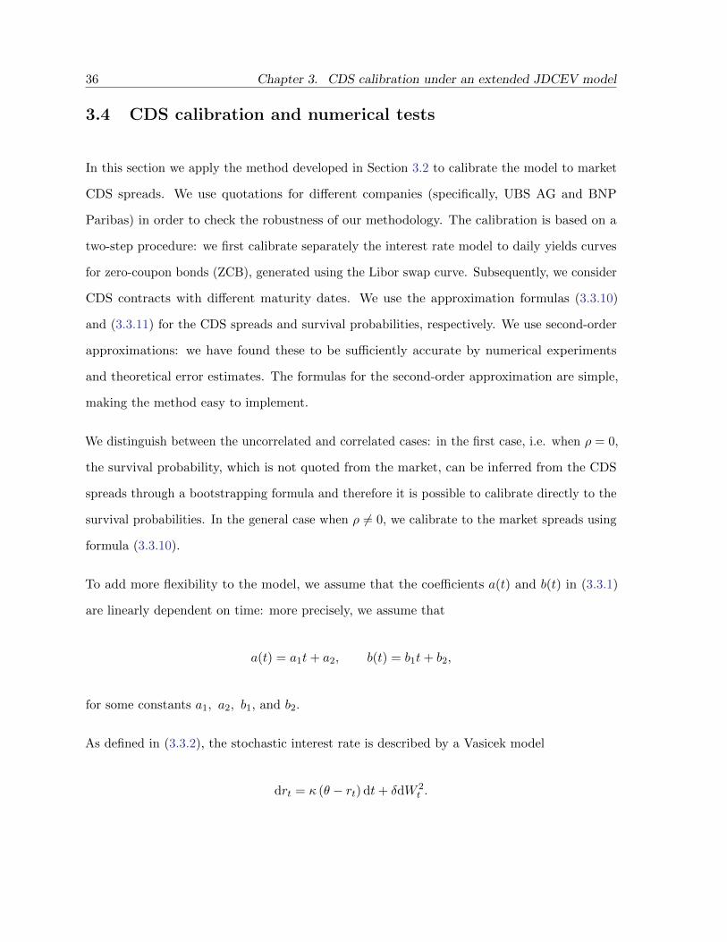
To add more flexibility to the model, we assume that the coefficients a(t) and b(t) in (3.3.1)
are linearly dependent on time: more precisely, we assume that
a(t) = a1t+ a2, b(t) = b1t+ b2,
for some constants a1, a2, b1, and b2.
As defined in (3.3.2), the stochastic interest rate is described by a Vasicek model
drt = κ (θ − rt) dt+ δdW 2t .

3.4. CDS calibration and numerical tests 37
Apart from its simplicity, one of the advantages of this model is that interest rates can take
negative values. For the calibration, we use the standard formula for the price Pt (T ) of a
T -bond, which we recall here for convenience:
Pt (T ) = At (T ) e−Bt(T )rt ,
where
At (T ) = e
(θ− δ2
2κ2
)(Bt(T )−T+t)− δ
2
4κBt(T )2
, Bt (T ) =1− e−κ(T−t)
κ.
The results of the interest rate calibration are given in Table 3.1.
Table 3.1: Calibration to ZCB.
Times to maturity (years) market ZCB model ZCB errors
1. 1.00229 1.00641 -0.410925 %2 1.00371 1.00844 -0.470717 %3 1.00333 1.00667 -0.333553 %4 1.00099 1.00165 -0.0660915 %5 0.995836 0.993987 0.185689 %6 0.987867 0.984129 0.378397 %7 0.977005 0.972476 0.463518 %8 0.963596 0.959441 0.431229 %9 0.948371 0.945363 0.317189 %10 0.933829 0.930451 0.361748 %
Calibration of the term structure formula of the ZCB to the marketvalues of the ZCB. The relative errors between the model and marketprices are reported as well. κ = 0.06, θ = 0.09, δ = 0.024, r0 = −0.009.
3.4.1 CDS calibration
The problem of calibrating the model (3.3.2) is formulated as an optimization problem. We
want to minimize the error between the model CDS spreads and the market CDS spreads. Our
approach is to use the square difference between market and model CDS spreads. This leads to

38 Chapter 3. CDS calibration under an extended JDCEV model
the nonlinear least squares method
infΘF (Θ) , F (Θ) =
N∑i=1
|Ri − Ri|2
R2i
,
where N is the number of spreads used, Ri is the market CDS spreads of the considered
reference entity observed at time t = 0 and Θ = (a1, a2, b1, b2, β, c, ρ), with
a2 ≥ 0, a1 ≥ −a2
T, b2 ≥ 0, b1 ≥ −
b2T
c > 0, β < 1 and − 1 < ρ < 1.
In order to calibrate our model to data from real market, we received data from Bloomberg for
two large credit derivatives dealers: UBS AG and BNP Paribas.
Calibration results
Here, we present the results of calibrating of the model to a set of data covering the period
from January, 1st, 2017 to January, 1st , 2023. In the Table 3.2 and the Table 3.4, we present
the results of the calibration of the model with ρ = 0 to market CDS spreads of UBS and
BNP Paribas. The Table 3.3 and the Table 3.5 show the results for the model with correlation
(ρ 6= 0). In both cases, we can see that the model gives very good fit to the market data,
particularly to the most liquid market CDS spreads (2Y, 3Y and 5Y maturities). However we
can still observe high relative errors for the BNP Paribas CDS spread with maturity 4 years
due to the market incompleteness or the non-liquidity of its 4Y maturity CDS observed at
January, 1st, 2017. The interesting fact is that the model gives very good fit to liquid market
CDS and this is confirmed, in Appendix 7.2, by more calibration tests on CDS spreads of other
different companies.
3.4. CDS calibration and numerical tests 39
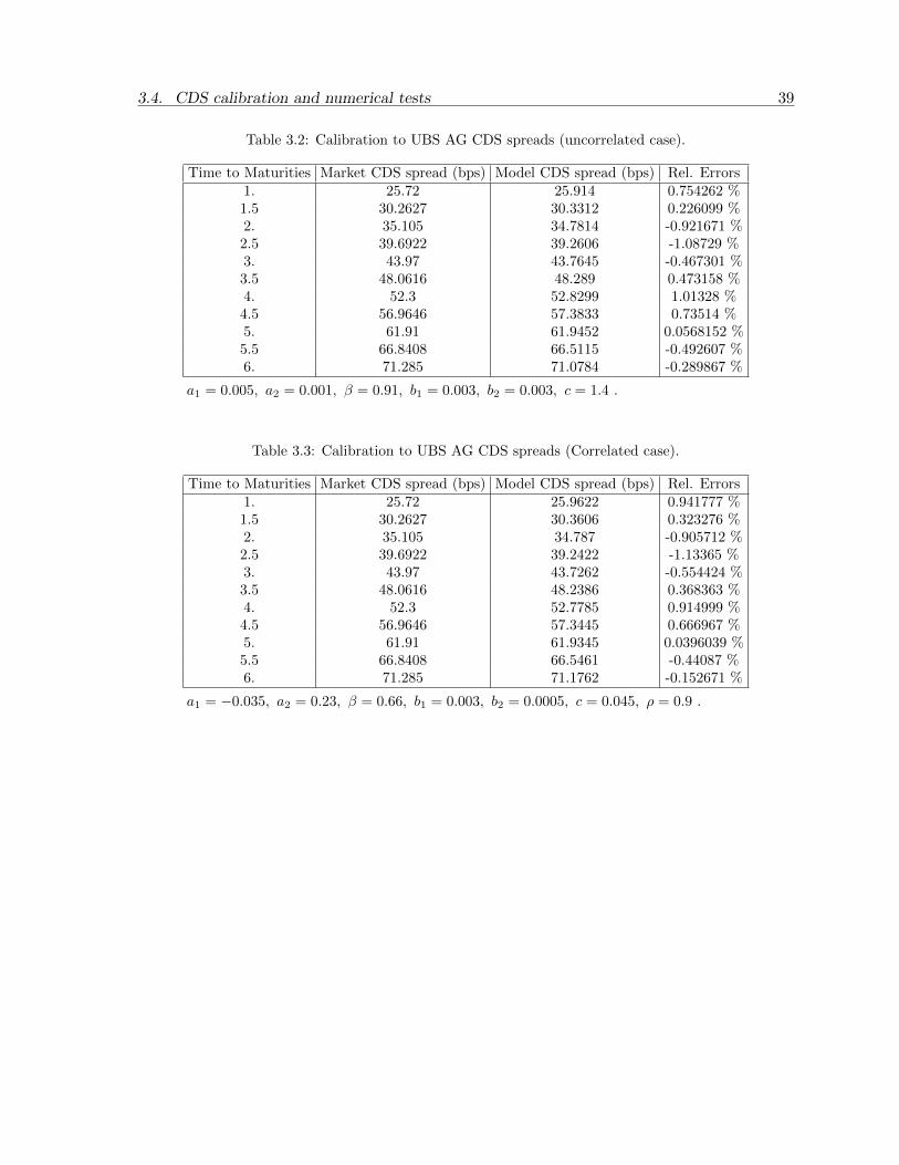
Table 3.2: Calibration to UBS AG CDS spreads (uncorrelated case).
Time to Maturities Market CDS spread (bps) Model CDS spread (bps) Rel. Errors1. 25.72 25.914 0.754262 %1.5 30.2627 30.3312 0.226099 %2. 35.105 34.7814 -0.921671 %2.5 39.6922 39.2606 -1.08729 %3. 43.97 43.7645 -0.467301 %3.5 48.0616 48.289 0.473158 %4. 52.3 52.8299 1.01328 %4.5 56.9646 57.3833 0.73514 %5. 61.91 61.9452 0.0568152 %5.5 66.8408 66.5115 -0.492607 %6. 71.285 71.0784 -0.289867 %
a1 = 0.005, a2 = 0.001, β = 0.91, b1 = 0.003, b2 = 0.003, c = 1.4 .
Table 3.3: Calibration to UBS AG CDS spreads (Correlated case).
Time to Maturities Market CDS spread (bps) Model CDS spread (bps) Rel. Errors1. 25.72 25.9622 0.941777 %1.5 30.2627 30.3606 0.323276 %2. 35.105 34.787 -0.905712 %2.5 39.6922 39.2422 -1.13365 %3. 43.97 43.7262 -0.554424 %3.5 48.0616 48.2386 0.368363 %4. 52.3 52.7785 0.914999 %4.5 56.9646 57.3445 0.666967 %5. 61.91 61.9345 0.0396039 %5.5 66.8408 66.5461 -0.44087 %6. 71.285 71.1762 -0.152671 %
a1 = −0.035, a2 = 0.23, β = 0.66, b1 = 0.003, b2 = 0.0005, c = 0.045, ρ = 0.9 .

40 Chapter 3. CDS calibration under an extended JDCEV model
Table 3.4: Calibration to BNP Paribas CDS spreads (uncorrelated case).
Time to Maturities Market CDS spread (bps) Model CDS spread (bps) Rel. Errors1. 34.615 34.0535 -1.62217 %1.5 39.8758 39.6736 -0.50717 %2. 45.115 45.4635 0.77257 %2.5 49.9935 51.4145 2.84236 %3. 56.11 57.517 2.50765 %3.5 64.5726 63.7612 -1.25665 %4. 72.59 70.1364 -3.38005 %4.5 77.6516 76.6317 -1.31333 %5. 82.27 83.2357 1.17384 %5.5 89.1455 89.9366 0.887389 %6. 96.705 96.7222 0.0177715 %
a1 = 0.018, a2 = 0.085, β = 0.88, b1 = 0.002, b2 = 0.0, c = 0.53
Table 3.5: Calibration to BNP CDS spreads (Correlated case).
Time to Maturities Market CDS spread (bps) Model CDS spread (bps) Rel. Errors1. 34.615 34.0073 -1.7557 %1.5 39.8758 39.6668 -0.524173 %2. 45.115 45.4813 0.811846 %2.5 49.9935 51.4436 2.90047 %3. 56.11 57.5465 2.56009 %3.5 64.5726 63.7827 -1.22334 %4. 72.59 70.1449 -3.36833 %4.5 77.6516 76.6259 -1.32086 %5. 82.27 83.2184 1.15283 %5.5 89.1455 89.9156 0.863835 %6. 96.705 96.7105 0.00566037 %
a1 = 0.023, a2 = 0.08, β = 0.6, b1 = 0.002, b2 = 0.002, c = 0.3, ρ = 0.96
For the calibration, we used a global optimizer, NMinimize, from Mathematica’s optimization
toolbox on a PC with 1× Intel i7-6599U 2.50 GHz CPU and 8GB RAM. We present in Table
3.6 the computational times of the calibration of the model to our two corporates in both
uncorrelated and correlated cases. One can conclude that the approximation formula (3.3.10)
gives an efficient and fast calibration.

3.4. CDS calibration and numerical tests 41
Table 3.6: Computational Times
Uncorrelated (second) Correlated (second)UBS AG 116.856 168.12
BNP Paribas 124.216 161.408
We check the results obtained from the calibration by computing the risk-neutral survival
probabilities with the approximation formula (3.3.11). In Tables 3.7 and 3.9, by comparing the
real market survival probability (column 2), our method (column 3) and the Monte Carlo (MC)
simulation (column 4), we observe that the method provides results as good as the MC. The
latter is performed with 100000 iterations and a confident interval of 95%. We do the same test
for the correlated case for both corporates and present the results in tables 3.8 and 3.10.
Table 3.7: Risk-neutral UBS AG survival probabilities (uncorrelated case).
Times to maturity Market probabilities Model probabilities Monte Carlo1. 0.995724 0.99569 [0.995704, 0.995704]2. 0.988367 0.988473 [0.988531, 0.988531]3. 0.978233 0.978335 [0.978468, 0.978468]4. 0.965644 0.965293 [0.965531, 0.965531]5. 0.949437 0.949391 [0.949765, 0.949766]6. 0.93056 0.930706 [0.931249, 0.93125]
Table 3.8: Risk-neutral UBS AG survival probabilities (correlated case).
Times to maturity model probability Monte Carlo1. 0.995724 0.995682 [0.995695, 0.995697]2. 0.988367 0.988471 [0.988523, 0.988528]3. 0.978233 0.978353 [0.978479, 0.978486]4. 0.965644 0.965324 [0.965553, 0.965563]5. 0.949437 0.949399 [0.949759, 0.94977]6. 0.93056 0.930619 [0.931142, 0.931152]

42 Chapter 3. CDS calibration under an extended JDCEV model
Table 3.9: Risk-neutral BNP Paribas survival probabilities (uncorrelated case).
Times to maturity Market probabilities Model probabilities Monte Carlo1. 0.994253 0.994339 [0.994358, 0.994359]2. 0.985077 0.984948 [0.98503, 0.985034]3. 0.972302 0.97157 [0.971779, 0.971788]4. 0.952539 0.954016 [0.954445, 0.954462]5. 0.933285 0.932175 [0.932925, 0.932955]6. 0.908874 0.906025 [0.907231, 0.90728]
Table 3.10: Risk-neutral BNP Paribas survival probabilities (correlated case).
Times to maturity market probability model probability Monte Carlo1. 0.994253 0.994347 [0.994363, 0.994368]2. 0.985077 0.98494 [0.985012, 0.985034]3. 0.972302 0.971544 [0.971742, 0.9718]4. 0.952539 0.953977 [0.95432, 0.954448]5. 0.933285 0.932115 [0.932728, 0.932973]6. 0.908874 0.9059 [0.906818, 0.907245]
However, as mentioned above in the Appendix (7.1.19), the convergence of the method is in the
asymptotic sense; that is it is asymptotically exact as the maturity goes to zero. To show the
dependence of the errors on the maturity, we plot the market and model survival probabilities
in function of maturity in Figure 3.2, T 7→ CDS(0, T ). The dotted lines correspond to the
survival probabilities computed with calibrated parameters and the continuous lines to the real
market survival probabilities. We observe that, after 6Y, the errors between the market and
model survival probabilities start increasing, as expressed by the error bounds (7.1.19).
(a) UBS AG Survival Probability (b) BNP Paribas Survival Probability
Figure 3.2: Dependence of the error on the maturity

3.4. CDS calibration and numerical tests 43
Influence of the correlation
To see the influence of the correlation in our model, we adopt the test done in [5]. Indeed
the authors consider four different payoffs that appear in credit derivatives and compare their
present values in very positive and negative correlation cases, i.e. ρ = 1 and ρ = −1.
A = D (0, 5Y )L (4Y, 5Y )1ζ<5Y , B = D (0, 5Y )1ζ<t,
C = D (0,min (ζ, 5Y )) , H = D (0, 5Y )L (4Y, 5Y )1ζ∈[4Y,5Y ],
where ζ is the time of default and L(S, T ) is the market LIBOR rate T > S. We consider the
UBS AG corporate. First we calibrate the model (3.3.2) to the UBS AG market CDS spreads
in both very positive and negative correlation cases. We obtain the following parameters:
ρ = 1 : a1 = 0.008, a2 = 0.008, β = 0.5, b1 = 0.003, b2 = 0.003, c = 0.68,
and
ρ = −1 : a1 = 0.006, a2 = 0.04, β = 0.624, b1 = 0.002, b2 = 0.0004, c = 1.325.
Table 3.11 shows, on one hand, that the correlation has no impact in the payoff of the form B
and C. Since the CDS spread and the risk-neutral survival probability expressions are written
as function in terms of B and C, the correlation has no influence in the computations of the
CDS spreads and the risk-neutral survival probabilities. On the other hand, higher effect can
be seen in the values of derivatives including LIBOR rates (A and H). This explains why in
both cases (non-correlation and correlation), our model gives a very good fit to the market
data. It follows that when we want to use the model for pricing derivatives of types A, H or

44 Chapter 3. CDS calibration under an extended JDCEV model
Table 3.11: Impact of the correlation
ρ = −1 ρ = 1 Rel. Errors Abs. ErrorsA 22.61 bps 90.986 bps +148.50% +0.00135B 505.482 bps 505.058 bps +0.083% +0.00004C 9947.149 bps 9948.279 bps -0.011% -0.00011D 16.244 bps -0.361 bps -548.883% 0.00019
pricing in general, it is better and much more accurate to consider the model with correlation.

Chapter 4
Numerical method for evalution of a
defaultable coupond bond
4.1 Introduction
The main objective of this chapter is to obtain the price of a defaultable coupon bond under
the extended Jump to Default Constant Elasticity of Variance (JDCEV) model proposed in
Chapter 3. From the mathematical point of view, the valuation problem of a defaultable coupon
bond can be posed in terms of a sequence of partial differential equation (PDE) problems,
where the underlying stochastic factors are the interest rates and the stock price. Moreover,
the stock price follows a diffusion process interrupted by a possible jump to zero (default), as it
is indicated previously. In order to compute the value of the bond we need to solve two partial
differential equation problems for each coupon and with maturities those coupon payment dates.
Concerning the numerical solution of those PDE problems, after a localization procedure to
formulate the problems in a bounded domain and the study of the boundaries where boundary
conditions are required following the ideas introduced in [36], we propose appropriate numerical
45

46 Chapter 4. Numerical method for evalution of a defaultable coupond bond
schemes based on a Crank-Nicolson semi-Lagrangian method for time discretization combined
with biquadratic Lagrange finite elements for space discretization. The numerical analysis of
this Lagrange-Galerkin method has been addressed in [3, 2]. Once the numerical solution of the
PDEs is obtained, a kind of post-processing is carried out in order to achieve the value of the
bond. This post-processing includes the computation of an integral term which is approximated
by using the composite trapezoidal rule.
This chapter is organized as follows. In Section 4.2, we present the mathematical modeling
with the PDE problem that governs the valuation of non callable defaultable coupon bonds. In
Section 4.3, we formulate the pricing problem in a bounded domain after a localization procedure
and we impose appropriate boundary conditions. Then, we introduce the discretization in time
of the problem by using a Crank-Nicolson characteristic scheme, and we state the variational
formulation of the problem in order to apply finite elements. Finally, in Section 4.4 we present
some numerical results to illustrate the good performance of the numerical methods and we
finish with some conclusions.
4.2 Model and PDE formulation for price of defaultable bond
Consider the following model introduced in Chapter 3
St = S0eXt1ζ≥t, S0 > 0,
dXt =(rt + b (t) +
(c− 1
2
)σ2 (t,Xt)
)dt+ σ (t,Xt) dW 1
t ,
drt = κ (θ − rt) dt+ δdW 2t ,
ζ = inft ≥ 0 |∫ t
0 λ (t,Xt) ≥ e,
dW 1t dW 2
t = ρdt,
(4.2.1)

4.2. Model and PDE formulation for price of defaultable bond 47
where S and r are, respectively, the defaultable stock price and the risk free interest rate and
σ (t, x) = a (t) e(β−1)x, with a, b, c and β defined as in Chapter 2. Consider a coupon bond
with maturity T , coupon rate (cpi, i = 1, · · · ,M) and recovery rate η. It consists of
A payment a coupon rate cpi at given dates ti if no default by ti, for i = 1, · · · , M where
M is the number of coupons and T = tM
A payment of a face value FV at maturity if no default occurs prior to T
A payment of a recovery rate η, in case of default before the maturity, at the default time
ζ.
The value V (t, S, r;T ) at time t > 0 of this bond is given by
V (t, S, r;T ) = FV · E
(M∑i=1
cpie−∫ tit rudu1ζ>ti + ηe−
∫ ζt rudu1ζ≤T + e−
∫ Tt rudu1ζ>T|Gt
)(4.2.2)
Proposition 4.2.1. Under the model (4.2.1), the value V (S, r;T ) := V (0, S, r;T ) at time
t = 0 of a bond with maturity T , coupon rates (cpi, i = 1, · · · ,M) and constant recovery rate η
is given by
V (S, r;T ) = FV
[M∑i=1
cpi E[exp
(−∫ ti
0
(ru + λ(u, Su)) du
)]+ E
[exp
(−∫ T
0
(ru + λ(u, Su)) du
)]
+η
(1− E
[exp
(−∫ T
0
(ru + λ(u, Su)) du
)]−∫ T
0
E[exp
(−∫ τ1
0
(ru + λ(u, Su)) du
)rτ1
]dτ1
)].
Proof. From (4.2.2) and with the Lemma 2.1.8 and 2.1.9, we have on ζ > t
V (t, S, r;T ) = FV
(M∑i=1
cpiE(e−
∫ tit rudu1ζ>ti|Gt
)+ ηE
(e−
∫ ζtrudu1ζ≤T|Gt
)+ E
(e−
∫ Ttrudu1ζ>T|Gt
))
= FV
(M∑i=1
cpiE(e−
∫ tit (ru+λu)du|Ft
)+ η
∫ T
t
E(e−
∫ st
(ru+λu)duλs|Ft)
ds+ E(e−
∫ Tt
(ru+λu)du|Ft))

48 Chapter 4. Numerical method for evalution of a defaultable coupond bond
⇒ V (S, r;T ) = FV
(M∑i=1
cpiE(e−
∫ ti0 (ru+λu)du
)+ η
∫ T
0
E(e−
∫ s0
(ru+λu)duλs
)ds+ E
(e−
∫ T0
(ru+λu)du))
The statement follows by replacing the following identities in the equality above:
e−∫ s0
(ru+λ(u,Xu))duλ(s,Xs) = − ∂∂s
(e−
∫ s0
(ru+λ(u,Xu))du)− rse−
∫ s0
(ru+λ(u,Xu))du,
and
∫ T
0
e−∫ s0
(ru+λ(u,Xu))duλ(s,Xs)ds = 1−
(e−
∫ T0
(ru+λ(u,Xu))du +
∫ T
0
e−∫ s0
(ru+λ(u,Xu))dursds
).
Next, if we denote by
u1(0, St, rt; s) = E[exp
(−∫ s
0(ru + λ(u, Su)) du
)],
u2(0, St, rt; τ1) = E[exp
(−∫ τ1
0(ru + λ(u, Su)) du
)rτ1
],
the expression of the bond value (4.2.1) can be written equivalently as
V (St, rt;T ) = FV
[M∑i=1
cpi u1(0, St, rt; ti) + u1(0, St, rt;T )
+η
(1− u1(0, St, rt;T )−
∫ T
0u2(0, St, rt; τ1) dτ1
)]. (4.2.3)
Moreover, applying the Feynman-Kac formula (see [39], for example) and by using the change
of variable yt = rt exp(κt), u1 and u2 are solutions of the Cauchy problem
(∂t + A)u(t, S, y) = 0, t < T1, (S, y) ∈ (0, ∞)× (−∞, ∞),
u(T1, S, y) = h(y), (S, y) ∈ (0, ∞)× (−∞, ∞),(4.2.4)

4.3. Numerical methods for picing defaultable bond 49
with h(y) = 1 for u = u1 or h(y) = exp(−κT1)y for u = u2, respectively. Moreover, the operator
A is defined as follows
(∂t + A)u = ∂tu+1
2σ2(t, S)S2 ∂SSu+ ρδσ(t, S) exp(κt)S ∂Syu+
1
2δ2 exp(2κt) ∂yyu
+ (exp(−κt)y + λ(t, S))S ∂Su+ κθ exp(κt) ∂yu− (exp(−κt)y + λ(t, S))u.
The existence of the solution to the Cauchy problem (4.2.4) in a bounded domain is ensured
and proved by Theorem 3.3.3.
4.3 Numerical methods for picing defaultable bond
In order to obtain a numerical approach of the value of a non callable defaultable coupon bond
we need to solve the Cauchy problem (4.2.4) for u = u1 and u = u2 with maturity T1 = ti for
i = 1, ...,M , that is each coupon payment date for both cases. Once these problems are solved,
the value of the bond is given by expression (4.2.3) in which appears an integral term. That
integral term will be approximated by means of the classical composite trapezoidal rule. For
the numerical solution of the PDE problem, we propose a Crank-Nicolson characteristics time
discretization scheme combined with a piecewise bi-quadratic Lagrange finite element method.
This Lagrange-Galerkin method has been analyzed in [3, 2] for time and space discretization.
More recently, it has been applied to the valuation of pension plans without and with early
retirement in [8] and [30], respectively. Thus, in order to apply this numerical technique, first a
localization procedure is used to cope with the initial formulation in an unbounded domain.
4.3.1 Localization procedure and formulation in a bounded domain
In this section we replace the unbounded domain by a bounded one. To determine the required
boundary conditions for the associated PDE problem we follow [36] based on the theory proposed

50 Chapter 4. Numerical method for evalution of a defaultable coupond bond
by Fichera in [13]. Let us introduce the following notation:
x0 = t, x1 = S and x2 = y.
Let x∞1 and x∞2 be two large enough real numbers and
Ω∗ = (0, x∞0 )×(
1
x∞1, x∞1
)× (−x∞2 , x∞2 )
with x∞0 = T1. Additionally, we make the changes of variables x1 = x1 − 1x∞1
, x2 = x2 + x∞2 ,
x∞1 = x∞1 − 1x∞1
and x∞2 = 2x∞2 . It follows a new bounded domain Ω defined as:
Ω = (0, x∞0 )× (0, x∞1 )× (0, x∞2 )
We denote the Lipschitz boundary by Γ = ∂Ω such that Γ =⋃2i=0(Γ−i ∪ Γ+
i ), where
Γ−i = (x0, x1, x2) ∈ Γ | xi = 0, Γ+i = (x0, x1, x2) ∈ Γ | xi = x∞i , i = 0, 1, 2.
Then, the operator defined in (4.2) can be written in the form:
Au =2∑
i,j=0
bij∂2u
∂xixj+
2∑j=0
bj∂u
∂xj+ b0u,
where the involved data are given by
B = (bij) =
0 0 0
0 12a
2(t)(x1 + 1
x∞1
)2β12ρδa(t)
(x1 + 1
x∞1
)βexp(κt)
0 12ρδa(t)
(x1 + 1
x∞1
)βexp(κt) 1
2δ2 exp(2κt)
,

4.3. Numerical methods for picing defaultable bond 51
b = (bj) =
1(
exp(−κt)(x2 − x∞2 ) + λ(t, x1 + 1
x∞1
))(x1 + 1
x∞1
)κθ exp(κt)
,
b0 = −(
exp(−κt)(x2 − x∞2 ) + λ
(t, x1 +
1
x∞1
)).
Thus, following [36], in terms of the normal vector to the boundary pointing inward Ω,
m = (m0,m1,m2), we introduce the following subsets of Γ:
ð0 =
x ∈ Γ/2∑
i,j=0
bijmimj = 0
, ð1 = Γ− ð0,
ð2 =
x ∈ ð0/
2∑i=0
bi − 2∑j=0
∂bij∂xj
mi < 0
.
As indicated in [36] the boundary conditions at ð1⋃ð2 for the so-called first boundary value
problem associated with (4.3.1) are required. Note that ð1 = Γ−1 , Γ+1 , Γ−2 , Γ+
2 and ð2 = Γ+0 .
Therefore, in addition to a final condition (see section 4.2), we need to impose boundary
conditions on Γ−1 , Γ+1 , Γ−2 and Γ+
2 . Next, we will impose Dirichlet conditions on Γ−1 , Γ−2 and
Γ+2 , whereas on Γ+
1 we will impose a homogeneous Neumann condition.
Taking into account the previous change of spatial variable and making the change of time
variable τ = T1 − t, we write the equation (4.2.4) in divergence form in the bounded spatial
domain Ω = (0, x∞1 ) × (0, x∞2 ). Thus, the initial boundary value problem (IBVP) takes the
following form:
Find u : [0, T1]× Ω→ R such that
∂τu−Div(A∇u) + v · ∇u+ lu = f in (0, T1)× Ω, (4.3.1)

52 Chapter 4. Numerical method for evalution of a defaultable coupond bond
u(0, .) = h(x2 − x∞2 ) in Ω,
u = exp
(−∫ T1
T1−τ
(exp(−κu)(x2 − x∞2 ) + λ
(u, x1 +
1
x∞1
))du
)h(x2 − x∞2 ) on (0, T1)× Γ−1 ,
∂u
∂x1= 0 on (0, T1)× Γ+
1 ,
u = exp
(−∫ T1
T1−τ
(exp(−κu)(x2 − x∞2 ) + λ
(u, x1 +
1
x∞1
))du
)h(x2 − x∞2 ) on (0, T1)× Γ−2 ,
u = exp
(−∫ T1
T1−τ
(exp(−κu)(x2 − x∞2 ) + λ
(u, x1 +
1
x∞1
))du
)h(x2 − x∞2 ) on (0, T1)× Γ+
2 ,
where the diffusion matrix A, the velocity field v, the reaction function l and the second
member f are defined as follows:
A =
12a
2(T1 − τ)(x1 + 1
x∞1
)2β12ρδa(T1 − τ)
(x1 + 1
x∞1
)βexp(κ(T1 − τ))
12ρδa(T1 − τ)
(x1 + 1
x∞1
)βexp(κ(T1 − τ)) 1
2δ2 exp(2κ(T1 − τ))
,
v =
12a
2(T1 − τ)(2β)(x1 + 1
x∞1
)2β−1−(
exp(−κ(T1 − τ)) (x2 − x∞2 ) + λ(T1 − τ, x1 + 1
x∞1
))(x1 + 1
x∞1
)12ρδa(T1 − τ)(β)
(x1 + 1
x∞1
)β−1exp(κ(T1 − τ))− κθ exp(κ(T1 − τ))
,
l = exp(−κ(T1 − τ))(x2 − x∞2 ) + λ
(T1 − τ, x1 +
1
x∞1
),
f = 0.

4.3. Numerical methods for picing defaultable bond 53
4.3.2 Time discretization
The method of characteristics is based on a finite differences scheme for the discretization of
the material derivative, i.e., the time derivative along the characteristic lines of the convective
part of the equation (4.3.1). The material derivative operator is given by
D
Dτ= ∂τ + v · ∇.
For a brief description of the method, we first define the characteristics curve through x = (x1, x2)
at time τ , X(x, τ ; s), which satisfies:
∂
∂sX(x, τ ; s) = v(X(x, τ ; s)), X(x, τ ; τ) = x. (4.3.2)
In order to discretize in time the material derivative in the Cauchy problem (4.3.1), let us
consider a number of time steps N , the time step δτ = T/N and the time mesh points τn = nδτ,
n = 0, 12 , 1,
32 , . . . , N .
The material derivative approximation by the characteristics method for both problems is given
by:
Du
Dτ=un+1 − un Xn
δτ,
where u = u1, u2 and Xn(x) = X(x, τn+1; τn). In this case, the solution of (4.3.2) is not
computed analytically. Instead, we consider numerical ODE solvers to approximate the
characteristics curves (see [3], for example). More precisely, we employ the second order
Runge-Kutta method.
Next, we consider a Crank-Nicolson scheme around(X(x, τn+1; τ), τ
)for τ = τn+ 1
2 . So, the
time discretized equation for u = u1, u2 can be written as follows:

54 Chapter 4. Numerical method for evalution of a defaultable coupond bond
Find un+1 such that:
un+1(x)− un(Xn(x))
δτ− 1
2Div(A∇un+1)(x)− 1
2Div(A∇un)(Xn(x))
+1
2(l un+1)(x) +
1
2(l un)(Xn(x)) = 0.
(4.3.3)
In order to obtain the variational formulation of the semi-discretized problem, we multiply
(4.3.3) by a suitable test function, integrate in Ω, use the classical Green formula :
∫ΩDiv(A∇un)(Xn(x))ψ(x)dx =
∫Γ(∇Xn)−T (x)n(x) · (A∇un)(Xn(x))ψ(x)dAx
−∫
Ω(∇Xn)−1(x)(A∇un)(Xn(x)) · ∇ψ(x)dx
−∫
ΩDiv((∇Xn)−T (x)) · (A∇un)(Xn(x))ψ(x)dx.
(4.3.4)
Note that, due to the characteristics curves can not be obtained analytically, the terms
(∇Xn)−1(x) and Div((∇Xn)−T (x)) in (4.3.4) are replaced by the following approximations
(see [3] for more detail):
(∇Xn)−1(x) = I(x) + δτLn(Xn(x)) +O(δτ2),
Div((∇Xn)−T (x)) = δτ ∇Div (vn(Xn(x))) +O(δτ2),
where L = ∇v.
After the previous steps, we can write a variational formulation for the time discretized problem

4.3. Numerical methods for picing defaultable bond 55
as follows:
Find un+1 ∈ H1(Ω) for all ψ ∈ H1(Ω) such that ψ = 0 on Γ−1 , Γ−2 and Γ+2 :
1
δτ
∫Ωun+1(x)ψ(x)dx +
1
2
∫Ω
(A∇un+1)(x) · ∇ψ(x)dx +1
2
∫Ω
(lun+1)(x)ψ(x)dx
=1
δτ
∫Ωun(Xn(x))ψ(x)dx− 1
2
∫Ω
(A∇un)(Xn(x)) · ∇ψ(x)dx
−δτ2
∫Ω
Ln(Xn(x))(A∇un)(Xn(x)) · ∇ψ(x)dx− 1
2
∫Ω
(lun)(Xn(x))ψ(x)dx
−δτ2
∫Ω∇Div (vn(Xn(x))) · (A∇un)(Xn(x))ψ(x)dx
+1
2
∫Γ(I(x) + δτLn(Xn(x)))Tn(x) · (A∇un)(Xn(x))ψ(x)dAx +
1
2
∫Γ+1
a12(x)∂u
∂x2(x)ψ(x)dAx,
where a12 is the corresponding coefficient of the diffusion matrix A.
4.3.3 Finite elements discretization
For the spatial discretization, we consider τh a quadratic mesh of the domain Ω. Let
(T2,Q2, σT2) be a family of piecewise quadratic Lagrangian finite elements, where Q2 denotes
the space of polynomials defined in T2 ∈ τh with degree less or equal than two in each spatial
variable and σT2 the subset of nodes of the element T2. More precisely, let us define the finite
elements space uh by
uh = φh ∈ C0(Ω) : φhT2 ∈ Q2, ∀T2 ∈ τh,
where C0(Ω) is the space of piecewise continuous functions on Ω.

56 Chapter 4. Numerical method for evalution of a defaultable coupond bond
4.3.4 Composite trapezoidal rule
In order to obtain the value of the bond at origination by means of expression (4.2.3) the
computation of an integral term is required. The approximation of this integral is carried out
by using a suitable numerical integration procedure. More precisely, we employ the classical
composite trapezoidal rule with M + 1 points, where M is the number of coupons, in the
following way:
∫ T
0u2(0, St, rt; τ1)dτ1 ≈
h
2
u2(0, St, rt; 0) + 2
M−1∑j=1
u2(0, St, rt; kj) + u2(0, St, rt;T )
where h = T
M , kj = jh for j = 1, ...,M − 1 and u2(0, St, rt; 0) = r0.
4.4 Empirical Results
In order to show the good performance of the numerical methods explained in Section 4.3, we
present some numerical results. In the following examples, the value of some of the parameters
involved in the underlying factors are obtained by applying the method introduced in Chapter
2. More precisely, first the interest rate model is calibrated to zero-coupon bonds (ZCB) and
next the model is calibrated to CDS spreads whose price is obtained by means of an asymptotic
expansion method.
In both examples, the number of elements and nodes of the finite element meshes employed in
the numerical solution of the problems are shown in Table 4.1.

4.4. Empirical Results 57
4.4.1 Example 1
First, we consider the simple case of the valuation of default-free zero-coupon bonds with
different maturities. In this setting, the valuation problem is reduced to a one-factor model.
The purpose of this example is to compare the value of the bonds we obtain with the market
zero-coupon curve. In order to obtain the value of the bonds, we solve the IBVP (4.3.1) with
initial condition h = 1 and only taking into account as underlying factor the interest rate. The
value of the parameters involved in the interest rate model are the ones collected in Table 4.2.
The values of the zero-coupon curve and the approximated ones obtained by solving the here
proposed model are presented in Table 4.3. For the numerical solution we consider Mesh 64
and the time step δτ = 1360 (one day).
Number of elements Number of nodes
Mesh 4 16 81
Mesh 8 64 289
Mesh 16 256 1089
Mesh 32 1024 4225
Mesh 64 4096 16641
Table 4.1: Different finite element meshes (number of elements and nodes).

58 Chapter 4. Numerical method for evalution of a defaultable coupond bond
Parameters of the defaultable stock price model
a1 = 0.0338a2 = 0.0524b1 = 0.0027b2 = 0.0028c = 0.0436
β = 0.731504,
Parameters of the interest rate model
κ = 0.0452δ = 0.0215θ = 0.1033
Correlation coefficient
ρ = 0.0
Initial conditions
S0 = 1.0r0 = −0.0092
Table 4.2: Parameters of the model for the UBS bond.
Maturity (years) Market ZCB Model ZCB
1 1.00229 1.006751
2 1.00372 1.009062
3 1.00333 1.007495
4 1.00099 1.002601
5 0.995825 0.994902
6 0.987805 0.984889
7 0.976833 0.973024
8 0.963223 0.959738
9 0.947687 0.945429
10 0.932845 0.930463
Table 4.3: Market and model values of the ZCB.
4.4.2 Example 2
Next, we consider the valuation of two real defaultable bonds traded in the market and issued
by different firms. On one hand, we take into account the pricing of a UBS bond quoted in

4.4. Empirical Results 59
Euro with maturity 5 years and a face value of 100. The bond pays annually coupon rates of
1.25 basis points and the recovery rate at the event of default is 40%. The model parameter
values for this example are collected in Table 4.2. In this case the correlation coefficient ρ is
assumed to be zero. Next, in Table 4.4 we present the value of the bond for different meshes
and time steps. In this case, we can appreciate that the price of the bond converges to 102.62.
On the other hand, we present a correlated case. More precisely, we address the valuation of
a JP Morgan(JPM) bond quoted in US Dollar with maturity 5 years and a face value of 100.
The bond pays annually coupon rates of 3.25 basis points and the recovery rate at the event of
default is again 40%. For this second example the parameter values of the model are the ones
which appear in Table 4.5. As we have just pointed out the correlation coefficient ρ is different
from zero. Finally, the value of this bond is shown in Table 4.6. In this case, the value of the
bond converges to 103.57.
In both cases, in order to obtain the value of the bond for we need to solve for each coupon
payment date the IBVP (4.3.1) with maturity those dates and with initial condition h = 1 or
h = exp(−κT )(x2 − x∞2 ). More precisely, in both examples the maturity of the bond is 5 years
and the frequency of coupon payments is annually, thus to obtain the value of the bond we
need to solve the problem (4.3.1) 10 times, i.e. 5 times with one initial condition to obtain the
value of u1 and 5 times with the other initial condition to obtain the value of u2.
Table 4.7 presents the a comparison of our pricing method to Monte Carlo Simulation in both
non callable defaultable coupon bonds. The Monte Carlo simulation is performed with 100000
iterations and a confident interval of 95%. Next, in Figures 4.1 and 4.2 we show the mesh value
of the UBS bond and the JP Morgan bond, respectively. Both figures are obtained with the
finer mesh and with time step δτ = 1360 (one day).

60 Chapter 4. Numerical method for evalution of a defaultable coupond bond
Time steps per year Mesh 4 Mesh 8 Mesh 16 Mesh 32 Mesh 64
90 102.499496 102.603837 102.616859 102.619028 102.618959
180 102.499599 102.605953 102.617976 102.619681 102.619602
360 102.500454 102.606351 102.618421 102.620069 102.619925
720 102.500663 102.606518 102.618587 102.620248 102.620094
Table 4.4: Value of the UBS bond for different meshes and time steps.
Parameters of the defaultable stock price model
a1 = 0.0313a2 = 0.0357b1 = 0.0004b2 = 0.0017c = 0.3466β = 0.777
Parameters of the interest rate model
κ = 0.1449δ = 0.0133θ = 0.0347
Correlation coefficient
ρ = 0.4971
Initial conditions
S0 = 1.0r0 = 0.0147
Table 4.5: Parameters of the model for the JP Morgan bond.
Time steps per year Mesh 4 Mesh 8 Mesh 16 Mesh 32 Mesh 64
90 103.725041 103.596891 103.572191 103.570225 103.570524
180 103.841153 103.605155 103.575270 103.572747 103.573144
360 103.794567 103.602389 103.576483 103.574147 103.574509
720 103.794298 103.602461 103.577110 103.574772 103.575161
Table 4.6: Value of the JP Morgan bond for different meshes and time steps.

4.4. Empirical Results 61
Step = 720 and Mesh = 64 Monte Carlo
UBS 102.620 [102.525, 102.727]
JPM 103.575 [103.556, 103.657]
Table 4.7: New method vs Monte Carlo simulation
Figure 4.1: Value of the UBS bond
Figure 4.2: Value of the JP Morgan bond

62 Chapter 4. Numerical method for evalution of a defaultable coupond bond

Chapter 5
Sovereign CDS calibration under a
hybrid Sovereign Risk Model
5.1 Introduction
Recent dynamics of sovereign credit risk in Europe have determined some significant doubts on
the paradigm considering a Euro area government bond as a risk free investment. Consequently
for investors the identification and pricing of sovereign bonds becomes a crucial issue. Main
factors determining this structural change are the following:
lack of a common economic and financial policy, with investors’ perception that the
economic and political convergence of the Euro area still require a long time;
target to stabilize government deficits constantly disregarded by governments with the
impossibility of financing infrastructural investments and difficulties in reforming the
social security system;
63

64 Chapter 5. Sovereign CDS calibration under a hybrid Sovereign Risk Model
slowdown in economic growth and interdependence between financial sector crisis and
sovereign risk for some countries;
contagion effect triggered by the PSI in Greece and hence extended to the entire Euro
system (aggravated by the downgrading of rating agencies) with a consequent increase in
the risk premium requested by investors.
In the second half of 2011, following the escalation of the sovereign debt crisis in the Euro area
and the contagion of tensions from the peripheral countries (Greece, Ireland and Portugal)
to the core countries of the Euro area, foreign demand for Eurozone debt has suffered a
major collapse involving the liquidation of outstanding positions in particular by institutional
investors. The central element that led to this substantial change in terms of asset allocation
was the perception that only a few Eurozone countries could be considered risk free; in addition,
there was the growing fear of the Euro break-up which helped to stimulate the dynamics of
cross-border capital outflow. During the period July - October 2011, foreign investors sold
Eurozone fixed income instruments for around 88 bln Euro against a 320 bln Euro inflow in
the first half of 2011. Japanese investors sold almost 98% of the Greek bonds and 61% of the
Portuguese bonds; in the same period the sale of Italian bonds was almost 10.5%. Starting
from the Lehman default event (September 2008), government bonds spreads have suffered a
dramatic widening phase both in countries with a weak public sector finance and in countries
considered to be safer. The volatility of the government bonds spread seems to reflect not only
the perceived default risk of the issuers but also some other new relevant factors:
Aggregate risk (change in monetary policy, global uncertainty, risk aversion);
Liquidity risk;
Country specific risk;

5.1. Introduction 65
Figure 5.1: Government Bonds Spread versus Bund

66 Chapter 5. Sovereign CDS calibration under a hybrid Sovereign Risk Model
Contagion and systematic risk;
Exchange rate risk.
The lack of models for the assessment of the component represented in the spread risk (eg Break
up Euro scenario) and the lack of measures deemed sufficiently robust to quantify sovereign
risk have led most investors to a hyper-prudent assessment of the situation, based on worst
case hypotheses, negatively distorting the dynamics of spreads.
Default statistics currently used to calibrate corporate credit ratings are not applicable to
sovereign risk. Furthermore, as reported in Moody’s Investor Service Sovereign Default and
Recovery Rates study [35], there is a very limited number of developed countries default events
in the last 30 years (Greece in March 2012 and December 2012, Cyprus in July 2013) and
consequently it is not possible to infer a consistent rating migration rates matrix for those
countries. Also statistics on recovery rates available on defaulted sovereign bonds are estimated
mainly with reference to emerging countries; the average recovery rates reported by Moody’s in
the sovereign default study is higher than the recovery rates for the two defaults of Greece in
2012 and for the one of Cyprus in 2013.
The need for banks and financial institutions to assess the risk associated with government
bonds exposures has posed the problem for asset managers, traders and risk managers to
determine how to assess sovereign default risk. There is no a specific standard in models used to
assess the sovereign default risk and practitioners make use of consolidated models developed for
corporate bonds. The two main families of models used to price and assess the risk of corporate
and sovereign bonds are reduced-form models and structural models. Whereas reduced-form
models are based on the specification of the risk-neutral default intensity and the fractional loss
model, the structural models focus on the behavior of the assets of the issuer and the relative
volatility compared to the value of the liabilities. Structural models have varied widely in their
implementation, starting from the original models developed by Black and Scholes (1973) and

5.1. Introduction 67
Merton (1974) and moving to more complex specifications making assumptions concerning
the capital structures of the issuers and including different types of debts and other form of
liabilities. While in structural models the default time is usually a predictable stopping time,
defined as the first hitting time to a certain barrier by the asset process, in the reduce form the
default time is a totally unpredictable stopping time modeled as the first jump of a Poisson
process with stochastic intensity.
In the reduced form models, thanks to one of the fundamental properties of jumps in Poisson
processes, the survival probabilities can be computed as a discount factors, and so it is a
common market practice to compute these probabilities from credit default swap market
information instead of the bond market. Moreover, the market of sovereign credit default swaps
(SCDS) contracts has grown very fast in the last decade and has become very liquid, clean and
standardized. So, the market of SCDS offers a consistent data framework set to estimate the
default-survival probabilities. Furthermore estimates retrieved from CDS market prices allow
practitioners to exclude the issue to represent the liquidity component of bonds spreads.
In this chapter we consider fixed Loss Given Default, that is a standard practice in the market
and supported by historical observation. Unlike corporate CDS contracts, SCDS are usually
denominated in a difference currency than the currency of the underling bonds. This is due
to avoiding the risk of depreciation of the bond’s currency in case of a credit event. In fact,
if SCDS were denominated in the same currency as the bond, the recovery value would be
significantly distorted by exchange rate fluctuation. So, for example, the market convention is
to trade Euro CDS in US dollar and US CDS in Euro. The different currency between SCDS
and bonds market makes it impossible to use the usual bootstrap technique to compute the
default-survival probabilities in the bond’s currency measure as for a corporate firm. Moreover,
the assumption that the foreign and domestic hazard rate are identical is not realistic and
contradicts market observations. So, the joint evolution of the domestic hazard rates and the
FX rate between the two currencies must be modeled.

68 Chapter 5. Sovereign CDS calibration under a hybrid Sovereign Risk Model
One of the motivations of this work has been to better understand the interrelationship between
the creditworthiness of a sovereign, its intensity to default and the exchange rate between
its bond’s currency and the currency in which SCDS contracts are quoted. We analyze the
differences between the default intensity under the domestic and foreign measure and we
compute the default-survival probabilities in the bond’s currency measure. Finally, we test our
calibration to the valuation of sovereign bonds even during the period of sovereign crisis.
We start by providing a robust and efficient method to calibrate a hybrid sovereign risk model
to SCDS market. We first present a model for the intensity of default of a sovereign government
based on the jump to default extended CEV (Constant Elasticity Variance) model introduced
in [9] in 2006 by establishing the link with the exchange rate. Then we give an approximation
formula to the SCDS spread obtained from perturbation theory.
Our approach is similar to [7] where the authors presented a model that captures the link
between the sovereign default intensity and the foreign exchange rate by adding a constant
in case of credit event to this exchange rate process. As shown in [12], the introduction of a
jump in the dynamics of the FX rate is necessary since a purely diffusion-based correlation
between the exchange rate the hazard rate is not able to explain market observations. The
default intensity is described by the exponential of some Ornstein-Uhlenbeck processes. Our
work differs from [7] in several aspects: first we provide a hybrid model that captures the
default intensity of the sovereign. Second, to approximate the SCDS spread, we employ a recent
methodology introduced in [29, 37], which consists in an asymptotic expansion of the solution
to the pricing partial differential equation. This approach of describing the sovereign default
intensity with a hybrid model has been introduced in [23]. The authors are also inspired by the
JDCEV model [9] which has been originally proposed for assessing corporate credit risks.
This chapter is organized as follows. In Section 5.2 we set the notations and introduce the
model. In Section 5.3 we recall the definitions, properties on SCDS spreads and provide an
explicit approximation formula. Section 5.4 contains the numerical test: we calibrate the model
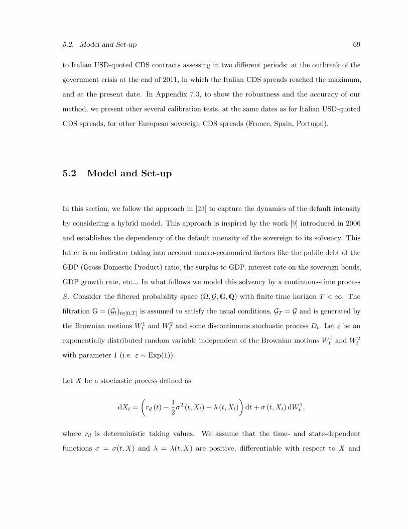
5.2. Model and Set-up 69
to Italian USD-quoted CDS contracts assessing in two different periods: at the outbreak of the
government crisis at the end of 2011, in which the Italian CDS spreads reached the maximum,
and at the present date. In Appendix 7.3, to show the robustness and the accuracy of our
method, we present other several calibration tests, at the same dates as for Italian USD-quoted
CDS spreads, for other European sovereign CDS spreads (France, Spain, Portugal).
5.2 Model and Set-up
In this section, we follow the approach in [23] to capture the dynamics of the default intensity
by considering a hybrid model. This approach is inspired by the work [9] introduced in 2006
and establishes the dependency of the default intensity of the sovereign to its solvency. This
latter is an indicator taking into account macro-economical factors like the public debt of the
GDP (Gross Domestic Product) ratio, the surplus to GDP, interest rate on the sovereign bonds,
GDP growth rate, etc... In what follows we model this solvency by a continuous-time process
S. Consider the filtered probability space (Ω,G,G,Q) with finite time horizon T < ∞. The
filtration G = (Gt)t∈[0,T ] is assumed to satisfy the usual conditions, GT = G and is generated by
the Brownian motions W 1t and W 2
t and some discontinuous stochastic process Dt. Let ε be an
exponentially distributed random variable independent of the Brownian motions W 1t and W 2
t
with parameter 1 (i.e. ε ∼ Exp(1)).
Let X be a stochastic process defined as
dXt =
(rd (t)− 1
2σ2 (t,Xt) + λ (t,Xt)
)dt+ σ (t,Xt) dW 1
t ,
where rd is deterministic taking values. We assume that the time- and state-dependent
functions σ = σ(t,X) and λ = λ(t,X) are positive, differentiable with respect to X and

70 Chapter 5. Sovereign CDS calibration under a hybrid Sovereign Risk Model
uniformly bounded. Let L be a real positive constant with L < eX0 . Let ζ be defined as
ζ = inft > 0 | eXt ≤ L ∧ inft ≥ 0 |∫ t
0λ(s,Xs)ds ≥ ε (5.2.1)
By definition, ζ is a G-stopping time.
Assumption 5.2.1. 1. The market is modelled by the filtered probability space (Ω,G,G,Qd)
defined above where Q := Qd is a domestic spot risk-neutral martingale measure and
G represents the quantity of information of the market and to which all processes are
adapted.
2. The time to default of the sovereign is the stopping time ζ defined in (5.2.1) and we define
the solvency S of the sovereign as follows:
St = S0eXt1ζ>t, S0 > 0.
Default happens when the solvency becomes worthless in one of these two ways. Either
the process eX falls below L via diffusion or a jump-to-default occurs from a value greater
than L, where L represents a threshold of the sovereign debt crisis. In what follows,
we denote by F = Ft, t ≥ 0 the filtration generated by the sovereign solvency and
by D = Dt, t ≥ 0 the filtration generated by the process Dt = 1ζ≤t. Eventually,
G = Gt, t ≥ 0, Gt = Ft ∨Dt is the enlarged filtration.
3. The rate of exchange between foreign currency cf and domestic currency cd is denoted
by Zt ≥ 0, ri are the short-term interest rates and Bi (t) = e∫ t0 ri(u)du the instantaneous
bank accounts in the respective currencies ci, i = d, f . For simplicity, we assume that
the domestic and foreign interest rates are deterministic and are function of time t.
Remark 5.2.2. One can notice that the definition of the solvency of the sovereign is similar to
the one of the defaultable stock prices of a corporate in the previous chapter. Indeed solvency

5.2. Model and Set-up 71
can be seen as the ”stock price” of a sovereign.
We assume that the rate of exchange Z, defining the value of unit of the foreign currency cf in
the domestic currency cd, satisfies a SDE of the form
dZt = µZt Zt−dt+ δ Zt−dW 2t + γ Zt−dDt, with dW 1
t dW 2t = ρdt, (5.2.2)
where δ > 0 and γ ∈ [0, 1] is the devaluation/revaluation rate of the FX process. The dynamics
(5.2.2) captures the dependency between the sovereign default risk and the rate of exchange,
first through the correlation ρ between the Brownian motion W 1 and W 2 and then via the
coefficient of devaluation/evaluation γ. Indeed, there is a jump on the rate of exchange at the
time of default ζ by
∆Zζ = γZζ−
That is at ζ, the foreign currency cf is evaluated/devaluated with respect to the domestic
currency cd in a jump fraction γ of the pre-default value of Z. Therefore the price in cd of the
foreign instantaneous bank account at time t is Bf (t)Zt. By Ito formula and (5.2.2)
d (Bf (t)Zt) = Bf (t) dZt + rf (t)Bf (t)Ztdt (5.2.3)
= rf (t)Bf (t)Ztdt+ µZt Bf (t)Ztdt+ δBf (t)ZtdW2t + γBf (t)ZtdDt
= Bf (t)Zt((rf (t) + µZt + γ (1−Dt)λ (t,Xt)
)dt+ δdW 2
t + γdMt
)where the process dMt = dDt− dAt is a martingale with At =
∫ t0 (1−Ds)λsds the compensator
of Dt.
Proposition 5.2.3. If the rate of exchange between the foreign and domestic currencies obeys
a stochastic differential equation (5.2.2), and if the riskless short-term rates of return in the
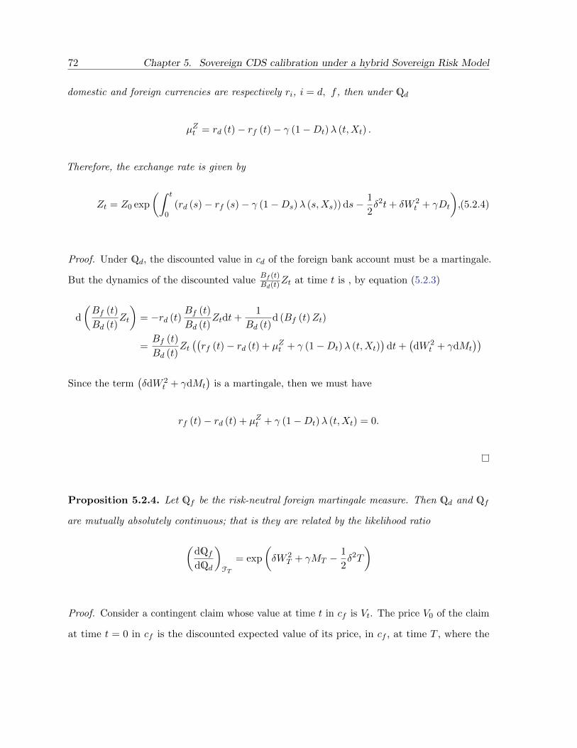
72 Chapter 5. Sovereign CDS calibration under a hybrid Sovereign Risk Model
domestic and foreign currencies are respectively ri, i = d, f , then under Qd
µZt = rd (t)− rf (t)− γ (1−Dt)λ (t,Xt) .
Therefore, the exchange rate is given by
Zt = Z0 exp
(∫ t
0(rd (s)− rf (s)− γ (1−Ds)λ (s,Xs)) ds− 1
2δ2t+ δW 2
t + γDt
),(5.2.4)
Proof. Under Qd, the discounted value in cd of the foreign bank account must be a martingale.
But the dynamics of the discounted valueBf (t)Bd(t)Zt at time t is , by equation (5.2.3)
d
(Bf (t)
Bd (t)Zt
)= −rd (t)
Bf (t)
Bd (t)Ztdt+
1
Bd (t)d (Bf (t)Zt)
=Bf (t)
Bd (t)Zt((rf (t)− rd (t) + µZt + γ (1−Dt)λ (t,Xt)
)dt+
(dW 2
t + γdMt
))Since the term
(δdW 2
t + γdMt
)is a martingale, then we must have
rf (t)− rd (t) + µZt + γ (1−Dt)λ (t,Xt) = 0.
Proposition 5.2.4. Let Qf be the risk-neutral foreign martingale measure. Then Qd and Qf
are mutually absolutely continuous; that is they are related by the likelihood ratio
(dQfdQd
)FT
= exp
(δW 2
T + γMT −1
2δ2T
)
Proof. Consider a contingent claim whose value at time t in cf is Vt. The price V0 of the claim
at time t = 0 in cf is the discounted expected value of its price, in cf , at time T , where the

5.2. Model and Set-up 73
expectation is computed under Qf , the risk-neutral foreign martingale measure:
V0 = e−∫ T0 rf (s)dsEf [VT ] . (5.2.5)
Let Ut be the time-t price of the claim in cd. Then Ut = VtZt, where Zt is the rate of exchange
between cf and cd. Since the claim is a tradable asset, its price in cd must be a martingale
under Qd. In particular the time-zero price is the discounted expected value of the time-T
price:
U0 = e−∫ T0 rd(s)dsEd [UT ]
V0Z0 = e−∫ T0 rd(s)dsEd [VTZT ]
V0 = e−∫ T0 rf (s)dsEd
[VTZTZ0
e−∫ T0 (rf (s)−rd(s))ds
].
Comparing equations (5.2.5) and (5.2.6) shows that
Ef (VT ) = Ed(VTZTZ0
e−∫ T0 (rf (s)−rd(s))ds
).
Since it holds for any non-negative GT -measurable random variable VT , it follows from (5.2.4)
that
(dQfdQd
)FT
=ZTZ0
e−∫ T0 rf (s)−rd(s)ds = exp
(δW 2
T + γMT −1
2δ2T
).
Set Yt = log (Zt). By Ito formula, the dynamics of Y is given by
dYt =
(µZt −
1
2δ2
)dt+ δ dW 2
t + γ dDt
=
(rd (t)− rf (t)− 1
2δ2 − γ (1−Dt)λ (t,Xt)
)dt+ δ dW 2
t + γ dDt.

74 Chapter 5. Sovereign CDS calibration under a hybrid Sovereign Risk Model
oAs in [9], we set the volatility of the solvency and the intensity of default as
σ(t,X) = a(t)e(β−1)X (5.2.6)
and
λ(t,X) = b(t) + c σ(t,X)2 = b(t) + c a(t)2e2(β−1)X (5.2.7)
where β < 1 and a(t) > 0 are the so-called elasticity parameter and scale function, while
b(t) ≥ 0 and c ≥ 0 govern the sensitivity of the default intensity with respect to the solvency.
Under Qd, it follows that the risk-neutral dynamics of the solvency St = St, t ≥ 0 is then
given by
St = S0eXt (1−Dt) , S0 > 0,
dXt =(rd (t)− 1
2σ2 (t,Xt) + λ (t,Xt)
)dt+ σ (t,Xt) dW 1
t ,
dYt =(rd (t)− rf (t)− 1
2δ2 − γ (1−Dt)λ (t,Xt)
)dt+ δ dW 2
t + γ dDt,
dDt = γ (1−Dt)λ (t,Xt) dt+ dMt, with M a martingale.
dW 1t dW 2
t = ρdt,
ζ = inft > 0 | eXt ≤ L ∧ inft ≥ 0 |∫ t
0 λ (t,Xt) ≥ ε.
(5.2.8)
we adopt a martingale modeling approach, in some sense similarly to what is usually done in
the theory of interest rate models. Since our market model is incomplete, we directly consider
a martingale dynamics for S. Even if our framework is completely different, the martingale
approach is also reminiscent of Carr&Linetsky’s model [9] where S represents the price of a
traded asset.

5.3. Sovereign Credit Default Swap spread 75
5.3 Sovereign Credit Default Swap spread
As presented in chaper 3, a CDS is an agreement between two parties, called the protection
buyer and the protection seller, typically designed to transfer to the protection seller the
financial loss that the protection buyer would suffer if a particular default event happened to
a third party, called the reference entity. The protection seller delivers a protection payment
to the protection buyer at the time of the default event. In exchange the protection buyer
makes periodic premium payments at time intervals α at the credit default swap rate up to
the default event or the expiry maturity, whichever comes first. The protection payment is the
specified percentage (1− η) of the CDS notional amount N (=1 by assumption), called default
recovery or loss-given-default, paid at default time. The valuation problem is to determine the
arbitrage-free CDS rate R that makes the present value of the CDS contract equal to zero. This
rate equates the present value of the protection payoff to the present value of all the premium
payments.
By Sovereign, we understand, from the definition given by the International Swaps and
Derivatives Association (ISDA), “any state, potential subdivision or government, or any agency,
instrumentality, ministry, department or other authority ( including ... central bank) thereof”.
Here, for simplicity, we consider sovereign governments. Hence a sovereign Credit Default Swap
is a CDS where the reference entity is a government. e.g Eurozone States Members. From
ISDA, a credit event in sovereign CDS contracts is induced among others by
Failure to pay : a sovereign fails to make a payment on its obligations (principle, coupons,
etc..) in an amount at least as large as the payment requirement beyond the period
allowed;
Restructuring : a sovereign alters the principle amount, coupon, currency, maturity or the
ranking in priority of repayment of an obligation;

76 Chapter 5. Sovereign CDS calibration under a hybrid Sovereign Risk Model
Repudiation/moratorium: a sovereign refuses to honor its obligation and declares a
moratorium.
Proposition 5.3.1. Consider a sovereign CDS contact settled in foreign currency with constant
default recovery (1 − η), spread R paid at premium dates ti, i = 1, 2, · · · , M , so that
α = ti−1 − ti =T
M. Then, at time t = 0, the spread R ≡ R (0, T ) is given by
R =(1− η)
∫ T0 E
d(eYs−Y0−
∫ s0 (rd(u)+λ(u,Xu))duλ(s,Xs)
)ds
TM
∑Mi=1E
d(eYti−Y0−
∫ ti0 (rd(u)+λ(u,Xu))du
) . (5.3.1)
Proof. By Lemma 2.1.8 and 2.1.9, the price of the SCDS at time t is given by
Vt (R) = Ef
(e−
∫ ζtrf (u)du (1− η)1ζ≤T −
M∑i=1
e−∫ tit rf (u)du T
MR1ζ>ti|Gt
)
= Ed
(e−
∫ ζtrf (u)du (1− η)Lξ1ζ≤T −
M∑i=1
e−∫ tit rf (u)du T
MRLti1ζ>ti|Gt
)(by change of measure)
= (1− η)Ed(Bf (t)
Bf (ζ)
Bf (ζ)ZζBd (t)
Bf (t)ZtBd (ζ)1ζ≤T|Gt
)− T
M
M∑i=1
Ed(Bf (t)
Bf (ti)
Bf (ti)ZtiBd (t)
Bf (t)ZtBd (ti)R1ζ>ti|Gt
)
= (1− η)Ed(ZζBd (t)
ZtBd (ζ)1ζ≤T|Gt
)− T
M
M∑i=1
Ed(ZtiBd (t)
ZtBd (ti)R1ζ>ti|Gt
)
= 1ζ>t (1− η)
∫ T
t
Ed(eYs−Yt−
∫ st
(rd(u)+λ(u,Xu))duλ(s,Xs)|Ft)
ds
− 1ζ>t TMR
M∑i=1
Ed(eYti−Yt−
∫ tit (rd(u)+λ(u,Xu))du|Ft
).
By definition, the market CDS spread R(t, T ) at time t is determined by the equation Vt (R (t, T )) = 0.
Hence on 1ζ>t, we have
R (t, T ) =(1− η)
∫ TtEd(eYs−Yt−
∫ st
(rd(u)+λ(u,Xu))duλ(s,Xs)|Ft)
ds
TM
∑Mi=1E
d(eYti−Yt−
∫ tit (rd(u)+λ(u,Xu))du|Ft
) .
It follows the equality (5.3.1).

5.3. Sovereign Credit Default Swap spread 77
We aim to give an explicit approximation formula to SCDS spread (5.3.1) based on an asymptotic
expansion technique introduced in [29, 39]. From Propositon 2.3.1, computing the expectations
in (5.3.1) equals to solving general backward Cauchy problems
(∂t + A)u (t, z) = 0, t < T, z ∈ Rd,
u (T, z) = h (z) , z ∈ Rd,
where A = A(t, z) is a (locally) parabolic differential operator of the form
A (t, z) =∑|α|≤2
aα (t, z)Dαz , t ∈ R+, z ∈ Rd, (5.3.2)
with
α = (α1, . . . , αd) , |α| =d∑i=1
αi, Dαz = ∂α1
z1 . . . ∂αdzd.
In our specific setting, we will consider A to be the infinitesimal generator of the stochastic
processes (X,Y ) in (5.2.8), whose precise expression in given in formula (5.3.2).
This leads to an explicit approximation formula for the SCDS spread (5.3.1).
Theorem 5.3.2. Let T be the expiry date of the SCDS contract settled in foreign currency
with constant default recovery (1− η), spread R paid at premium dates ti, i = 1, 2, · · · , M , so
that α = ti−1− ti = TM . Under the general dynamics (5.2.8), there exist sequences of differential
operators(L
1,(x,y)n
)n≥0
and(L
2,(x,y)n
)n≥0
of the form of (7.1.11) and acting on (x, y) such that
the N -th order approximation of the SCDS spread in (5.3.1) is given by
RN =
(1− η)∫ T
0
N∑n=0
L1,(x,y)n (0, s)u0 (0, x, y; s) ds
TK
K∑i=1
N∑n=0
L2,(x,y)n (0, ti) v0 (0, x, y; ti)
, (5.3.3)

78 Chapter 5. Sovereign CDS calibration under a hybrid Sovereign Risk Model
where
u0 (0, x, y, s) = e−∫ s0 (rf (u)+ 1
2δ2+λ(u,x))du
·(b (s) + c a (s)2 exp
(2 (β − 1)
(x+
∫ s
0
(rd (u) +
(β − 3
2
)σ (u, x)2 + λ (u, x)
)du
)))v0 (0, x, y; s) = e−
∫ s0 (rf (u)+ 1
2δ2+2λ(u,x))du.
Proof. We see from (5.3.1) that we have to evaluate expectations of the form
Ed(eYT−Yt−
∫ Tt (rd(u)+λ(u,Xu))duh (XT , YT ) |Ft
).
They are functions of t,Xt, Yt and Dt. Let us denote its value at time t for Xt = x, Yt = y and
Dt = d as f (t, x, y, d). Set g (t, x, y, d) the value at time t = 0 of
Ed(eYT−
∫ T0 (rd(u)+λ(u,Xu))duh (XT , YT )
).
By Ito formula and its martingale property, one can see that
∂tf (t, x, y, d) +
(rd (t)− 1
2σ (t, x)2 + λ (t, x)
)∂xf (t, x, y, d) +
1
2σ (t, x)2 ∂2
xf (t, x, y, d)
+
(rd (t)− rf (t)− 1
2δ2 + γ (1− d)λ (t, x)
)∂yf (t, x, y, d) +
1
2δ2∂2
yf (t, x, y, d) + ρδσ (t, x) ∂xyf (t, x, y, d)
+ (1− d)λ (t, x) (f (t, x, y, 1)− f (t, x, y, 0)) +
(−rf (t)− 1
2δ2 − λ (t, x)
)f (t, x, y, d) = 0.
Set
u (t, x, y) = f (t, x, y, 1) and v (t, x, y) = f (t, x, y, 0)
⇒ f (t, x, y, d) = 1d=1u (t, x, y) + 1d=0v (t, x, y)

5.3. Sovereign Credit Default Swap spread 79
For the premium leg, the final conditions of u and v are
u (T, x, y) = f (T, x, y, 1) = 0,
v (T, x, y) = f (T, x, y, 0) = h (x, y) = 1.
u is solution to the PDE
(∂t +
(rd (t)− 1
2σ (t, x)2 + λ (t, x)
)∂x +
1
2σ (t, x)2 ∂2
x +
(rd (t)− rf (t)− 1
2δ2
)∂y+
+1
2δ2∂2
y + ρδσ (t, x) ∂xy +
(−rf (t)− 1
2δ2 − λ (t, x)
))u = 0, for t < T and x, y ∈ R2
u (T, x, y) = 0 x, y ∈ R2.
It follows that u ≡ 0. Therefore , for computing the premium leg, one only need to solve
directly the PDE for v
(∂t +
(rd (t)− 1
2σ (t, x)2 + λ (t, x)
)∂x +
1
2σ (t, x)2 ∂2
x +
(rd (t)− rf (t)− 1
2δ2 + γλ (t, x)
)∂y+
+1
2δ2∂2
y + ρδσ (t, x) ∂xy +
(−rf (t)− 1
2δ2 − 2λ (t, x)
))v = 0, for t < T and x, y ∈ R2
v (T, x, y) = 1 x, y ∈ R2.
Analogously , to compute the protection leg, one solve the following PDE for u
(∂t +
(rd (t)− 1
2σ (t, x)2 + λ (t, x)
)∂x +
1
2σ (t, x)2 ∂2
x +
(rd (t)− rf (t)− 1
2δ2
)∂y+
+1
2δ2∂2
y + ρδσ (t, x) ∂xy +
(−rf (t)− 1
2δ2 − λ (t, x)
))u = 0, for t < T and x, y ∈ R2
u (T, x, y) = λ (T, x) x, y ∈ R2.
Hence to approximate the Quanto CDS spread, we must deal with two Cauchy problems with

80 Chapter 5. Sovereign CDS calibration under a hybrid Sovereign Risk Model
different operators A1 and A2 and different terminal conditions:
(∂t + A1
)u (t, x, y) = 0, t < T, x, y ∈ R
u (T, x, y) = λ (T, x) , x, y ∈ R,(5.3.4)
and (∂t + A2
)v (t, x, y) = 0, t < T, x, y ∈ R
v (T, x, y) = 1, x, y ∈ R,(5.3.5)
where
A1 =1
2σ (t, x)2 ∂2
x + ρδσ (t, x) ∂xy +1
2δ2∂2
y +
(rd (t)− 1
2σ (t, x)2 + λ (t, x)
)∂x
+
(rd (t)− rf (t)− 1
2δ2
)∂y −
(rf (t) +
1
2δ2 + λ (t, x)
)
and
A2 =1
2σ (t, x)2 ∂2
x + ρδσ (t, x) ∂xy +1
2δ2∂2
y +
(rd (t)− 1
2σ (t, x)2 + λ (t, x)
)∂x
+
(rd (t)− rf (t)− 1
2δ2 + γλ (t, x)
)∂y −
(rf (t) +
1
2δ2 + 2λ (t, x)
).
Hence by Theorem 7.1.3, there exists a sequence (L1,(x,y)n )b≥n of differential operators such that
the N-th approximation of the solution u of (5.3.4) is given by
u (0, x, y; s) =N∑n=0
L1,(x,y)n (0, s)u0 (0, x, y; s) ,
where
u0 (0, x, y; s) = e∫ s0 χ(u,x,y)du
∫R2
Γ0 (0, x, y; s, ξ1, ξ2)λ (s, ξ1) dξ1dξ2,

5.3. Sovereign Credit Default Swap spread 81
with
χ (u, x, y) = −(rf (u) +
1
2δ2 + λ (u, x)
)
and Γ0 is the probability density of the 2-dimensional Gaussian random variable (Ξ1,Ξ2) with
covariance and mean respectively given by
C (0, x, y; s) =
∫ s0 σ (u, x)2 du ρδ
∫ s0 σ (u, x) du
ρδ∫ s
0 σ (u, x) du δ2 ∗ s
and
m (0, x, y; s) =
(x+
∫ s0
(rd (u)− 1
2σ (u, x)2 + λ (u, x))
du, y +∫ s
0
(rd (u)− rf (u)− 1
2δ2)
du
),
∫R2
Γ0 (0, x, y; s, ξ1, ξ2)λ (s, ξ1) dξ1dξ2 =
∫R
Γ0 (0, x; s, ξ1)λ (s, ξ1) dξ1,
where Γ0 is the marginal probability density function of the random Gaussian random variable
Ξ1 with variance and mean
C (0, x, y; s) =
∫ s
0σ (u, x)2 du
and
m (0, x, y; s) = x+
∫ s
0
(rd (u)− 1
2σ (u, x)2 + λ (u, x)
)du.
It follows
∫R
Γ0 (0, x; s, ξ1)λ (s, ξ1) dξ1 = b (s) + c a (s)
∫R
Γ0 (0, x; s, ξ1) e2(β−1)ξ1dξ1
= b (s) + c a (s)Ed [Π] ,

82 Chapter 5. Sovereign CDS calibration under a hybrid Sovereign Risk Model
where Π = e2(β−1)Ξ1 is a log-normal distributed random variable with mean Ed[Π] equals to
Ed (Π) = exp
(2 (β − 1)m (0, x, y; s) + 4 (β − 1)2 C (0, x, y; s)
2
)= exp
(2 (β − 1)
(m (0, x, y; s) + (β − 1)C (0, x, y; s)
))= exp
(2 (β − 1)
(x+
∫ s
0
(rd (u)− 1
2σ (u, x)2 + λ (u, x)
)du+ (β − 1)
∫ s
0σ (u, x)2 du
))= exp
(2 (β − 1)
(x+
∫ s
0
(rd (u) +
(β − 3
2
)σ (u, x)2 + λ (u, x)
)du
)).
Hence
u0 (0, x, y, s) = e−∫ s0 (rf (u)+ 1
2δ2+λ(u,x))du×
×(b (s) + c a (s)2 exp
(2 (β − 1)
(x+
∫ s
0
(rd (u) +
(β − 3
2
)σ (u, x)2 + λ (u, x)
)du
))).
Analogously, we see from theorem 7.1.3 that there exists a sequence (L2,(x,y)n )b≥n of differential
operators such that the N-th approximation of the solution v of (5.3.5) is given by
v (0, x, y; s) =N∑n=0
L2,(x,y)n (0, s) v0 (0, x, y; s) ,
where
v0 (0, x, y; s) = e∫ s0 χ(u,x,y)du
∫R2
Γ0 (0, x, y; s, ξ1, ξ2) dξ1dξ2 = e∫ s0 χ(u,x,y)du
with
χ (u, x, y) = −(rf (u) +
1
2δ2 + 2λ (u, x)
).

5.4. Sovereign CDS calibration and empirical test 83
5.4 Sovereign CDS calibration and empirical test
In this section we apply the method developed in Section 5.3 to calibrate the model (5.2.8) to
the sovereign CDS spreads quoted by the market. We use quotations for Italian USD-quoted
CDS provided by Bloomberg database on the date November, 15th 2011 in order to check the
robustness of our methodology. We use the second-order approximation formula (5.3.3) for
the SCDS. We consider SCDS contracts with maturity from one up to four years and paid
quarterly with recovery rate 40% at the event of default.
Since the formula (5.3.3) gives the approximation of the SCDS spread in the domestic currency
cd (EUR) and the market SCDS is in the foreign currency cf (USD), we consider the following
formula introduced in [7]:
R =R
1 + γ,
where R is SCDS spread in the USD. This shows the link between the SCDS spreads in two
currencies. To add more flexibility to the model, we assume that the coefficients a(t) and b(t)
in (5.2.7) are linearly dependent on time: more precisely, we assume that
a(t) = a1t+ a2, b(t) = b1t+ b2,
for some constants a1, a2, b1, and b2. The problem of calibrating the model (5.2.8) is formulated
as an optimization problem. We want to minimize the error between the model CDS spread
and the market CDS spreads. Our approach is to use the square difference between market and
model CDS spreads. This leads to the nonlinear least squares method
infΘF (Θ) , F (Θ) =
N∑i=1
|Ri − Ri|2
R2i
,

84 Chapter 5. Sovereign CDS calibration under a hybrid Sovereign Risk Model
where N is the number of spreads used, Ri is the market CDS spreads of the considered
reference entity observed at time t = 0 and Θ = (a1, a2, b1, b2, β, c, δ, ρ, γ), with
a2 ≥ 0, a1 ≥ −a2
T, b2 ≥ 0, b1 ≥ −
b2T, c ≥ 0, δ ≥ 0, β < 1, −1 < γ < 1 and − 1 < ρ < 1.
For the calibration, we use a global optimizer, NMinimize, from Mathematica’s optimization
toolbox on a PC with 1× Intel i7-6599U 2.50 GHz CPU and 8GB RAM. First we calibrate
the model to real market SCDS spreads taken at the outbreak of the government crisis at the
end of 2011. Table 5.1 shows the results of the calibration to Italian SCDS contracts settled in
USD and we can observe that the model gives very good fit to the real market data with a
computational time equals to 45.808 seconds. We calibrate our model to market data quoted at
November, 15th, 2011, when the Italian CDS spreads reached their maximum value.
Table 5.1: Calibration to Italy USD CDS quoted as COB November, 15th, 2011
Times to maturity (Year) Market spreads (bps) Model spreads (bps) Rel. errors1.25 639.604 641.307 0.266268 %1.5 634.042 627.823 -0.98089 %1.75 617.96 615.888 -0.335402 %2. 601.52 605.829 0.71629 %
2.25 592.68 597.979 0.894177 %2.5 590.589 592.642 0.347765 %2.75 592.193 590.018 -0.367292 %3. 594.44 590.072 -0.734818 %
3.25 594.935 592.299 -0.442919 %3.5 593.917 595.317 0.235591 %3.75 592.288 596.172 0.655759 %4. 590.945 589.227 -0.290722 %
a1 = 0.5, a2 = 0.2, β = −0.77, b1 = −0.014, b2 = 0.056, c = 0.015, δ = 0.94 ρ =−0.41, γ = 1.0, 45.808 seconds
We follow the same process as above but this time we calibrate to Italian SCDS spreads quoted
on May, 05th 2017. Table 5.2 shows that the method still provides very good fit to real market
data.

5.4. Sovereign CDS calibration and empirical test 85
Table 5.2: Calibration to Italy USD CDS quoted as COB May, 30th 2017
Times to maturity (Year) Market spreads (bps) Model spreads (bps) Rel. errors1.25 77.3576 78.0834 0.938368 %1.5 88.3681 87.4887 -0.995104 %1.75 97.1146 96.3335 -0.804301 %2. 104.695 104.63 -0.0616158 %
2.25 112.006 112.395 0.346509 %2.5 119.142 119.642 0.419618 %2.75 125.994 126.39 0.314503 %3. 132.455 132.658 0.15294 %
3.25 138.435 138.46 0.0180013 %3.5 143.918 143.811 -0.0747112 %3.75 148.906 148.714 -0.128773 %4. 153.4 153.161 -0.15609 %
a1 = 0.2, a2 = 0.03, β = 0.63, b1 = 0.01, b2 = 0.002, c = 0.005, δ = 1.068, ρ =0.24, γ = 0.54, 41.992 seconds
At time t = 0, the foreign survival probability of the SCDS is given by
pf0 (T ) = Ef(e−∫ T0 λf (u,Xu)du
)= Ef
(e−(1+γ)
∫ T0 λ(u,Xu)du
),
where λf is the default intensity in the foreign economy and is linked to the domestic default
intensity by the relation λf (t,Xt) = (1 + γ)λ (t,Xt). The dynamics of the underlying process
X in the foreign risk-neutral measure Qf is
dXt =
(rd (t)− 1
2σ2 (t,Xt) + λ (t,Xt)− ρησ (t,Xt)
)dt+ σ (t,Xt) dW 1
t ,
where W 1 is given by
dW 1t = dW 1
t −d〈W 1, Z〉t
Zt= dW 1
t − ρηdt.
By Feynman-Kac representation formula, pf0 (T ) = u (0, x;T ), where u is solution to the Cauchy

86 Chapter 5. Sovereign CDS calibration under a hybrid Sovereign Risk Model
problem
(∂t + A)u (t, x) = 0, t < T, x ∈ R,
u (T, x) = 1, x ∈ R,
with
A =1
2σ (t, x)2 ∂2
x +
(rd (t)− 1
2σ (t, x)2 + λ (t, x)− ρησ (t, x)
)∂x − λ (t, x) .
By Theorem 7.1.3, there exists a sequence of operator (Lxn)n≥0, acting on the variable x, such
that
pf0 (T ) = u (0, x) ≈ uN (0, x;T ) =N∑n=0
Lxn (0, T )u0 (0, x;T ) , (5.4.1)
where u0 is given by
u0 (t, x;T ) = e−(1+γ)∫ Tt λ(s,x)ds.
In Figures 5.3 and 5.2 we present a comparison between the expansion approximation method
and Monte Carlo simulation by computing the foreign survival probabilities (5.4.1) of Italy
USD CDS quoted as COB November, 15th, 2011 (Table 5.1) and Italy USD CDS quoted as
COB May, 30th 2017 (Table 5.2). The Monte Carlo is performed with 100000 iterations and
a confident interval of 95%. As mentioned in the Appendix (7.1.19), the convergence of the
method is in the asymptotic sense. Up to four years maturity, the method coincides with the
Monte Carlo simulation. After then, we can see that the curves of the survival probabilities
(dashed line) start moving away from the Monte Carlo confidence intervals (blue line).

5.4. Sovereign CDS calibration and empirical test 87
Figure 5.2: SCDS foreign Survival Probabilities of Italy USD CDS quoted as COB November,15th, 2011
Figure 5.3: SCDS foreign Survival Probabilities of Italy USD CDS quoted as COB May, 30th2017
To show the accuracy of the method, we present, in the Appendix 7.3, further calibration tests
of the model on SCDS of sovereigns belonging to Eurozone (cf. 7.3). In particular, we consider
the same dates used for the calibration tests to Italian CDS spreads, and we calibrate our model
to French, Spanish and Portuguese USD-quoted CDS spreads.

88 Chapter 5. Sovereign CDS calibration under a hybrid Sovereign Risk Model

Chapter 6
Conclusion
The main objectives of this dissertation are to enrich existing models and to provide new
calibration and pricing techniques in order to give more realistic descriptions of the financial
market in the wake up of the global crisis 2007/2009. With respect to the research questions
outlined in the introduction, the following summary gives an overview of the main findings.
In Chapter 3, we have proposed a new methodology for the calibration of a hybrid credit-equity
model to credit default swap (CDS) spreads and survival probabilities. We have considered
the Jump to Default Constant Elasticity Variance model in a more general framework. More
precisely, we assume that the interest rate is stochastic, correlated to the defaultable stock
price and can possibly take negative values. In order to calibrate the model, we have derived
an approximate analytic expression of the CDS spread (and the survival probability) based
on an asymptotic approximation of solutions to parabolic partial differential equations. The
numerical test on different corporates have shown that our method gives very good fit to real
market data for short maturities, i.e. up to six years maturity. Moreover we have seen this
approximation formula give an efficient and fast calibration to the market CDS spreads, in
both correlated and uncorrelated models.
89

90 Chapter 6. Conclusion
In Chapter 4, we have considered the valuation of a non callable and callable defaultable coupon
bond where the underlying stochastic factors are the interest rate and the defaultable stock
price follow the extended JDCEV model introduced in Chapter 3. In the case of non callable
bond, the pricing problem is posed as a sequence of IBVPs. More precisely, two PDE problems
with different initial conditions with maturity each coupon payment date need to be solved.
Once the numerical solution of these problems is carried out, the value of the bond is computed
by means of an expression which also involves the computation of an integral term.
To obtain a numerical solution of the PDE problems, we have proposed appropriate numerical
methods based on Lagrange-Galerkin formulations. More precisely, we combine a Crank-Nicolson
semi-Lagrangian scheme for time discretization with biquadratic Lagrange finite elements for
space discretization. Moreover, the integral term which is involved in the computation of the
bond value is approximated by means of the classical composite trapezoidal rule. Finally, we
show some numerical results in order to illustrate the behavior of the proposed methods. we
obtained very good approximations as shown in Table 4.7 which compare the method to Monte
Carlo simulation.
In Chapter 5, we have presented a hybrid sovereign risk model in which the intensity of default
of the sovereign is based on the jump to default extended CEV model with a deterministic
interest rate. We have assumed that the solvency of a sovereign follows the Jump to Default
Constant Elasticity Variance model introduced in [9]. The model captures the interrelationship
between creditworthiness of a sovereign, its intensity to default and the correlation with the
exchange rate between the bond’s currency and the currency in which the CDS spread are
quoted. We have analyzed the differences between the default intensity under the domestic and
foreign measure and we have computed the default-survival probabilities in the bond’s currency
measure. We have also given an approximation formula to sovereign CDS spread obtained by
using the same technique as in the Chapter 3. The numerical test on Republics of Italy, France,
Portugal and Spain have shown that the model gives a very good fit to real market data, both

91
at the outbreak of the government crisis and at the present date.
With regard to future research, a relevant question to address is if these model and CDS
approximation give good results for a dynamic CDS quote. Therefore, further empirical
research is needed to extend the approximation technique introduced in this dissertation.
Furthermore, it will be highly relevant to apply the numerical method in Chapter 4 on callable
defaultable bonds. i.e a bond with an embedded call option. Indeed, instead of parabolic partial
differential equations, we would face to obstacle problems. By definition, for a callable bond
the issuer preserves the right to call back the bond and pay a fixed price for it. When interest
rates decline (bond prices rise) after the initial issue, the firm can refund the bonds at the fixed
price instead of the market value. Then, adding the call option to a bond should make it less
attractive to buyers, since it reduces the potential upside on the bond. As interest rates go
down, and the bond price increases, the bonds are more likely to be called back.
Let us assume that the defaultable coupon bond introduced in Chapter 4 now contains a call
option with R = tc, · · · , TM the set of all possible call dates and [0, tc] the protection period.
At the time of call t ∈ R, the issuer re-purchases the bond from the bondholder for a call price
K (t). We denote by Ψ the payoff to the bondholder at maturity T. Let T be the set of all
F-stopping time. We define
Tt,T = τ ∈ T : τ ∈ [t, T ] a.s.
Let τ ∈ Tt∨tc,T be the time modelling the time of call by the issuer. From [26] one can see that
the t-value of the bond assuming that no default occurs prior to t is given by
V (τ ; t, S, r) = E
[exp
(−∫ T
t(ru + λ (u, Su)) du
)Ψ (ST )1T≤τ|Ft
]

92 Chapter 6. Conclusion
+ FV · E
[M∑i=1
exp
(−∫ ti
t(ru + λ (u, Su)) du
)ci1ti<τ|Ft
]
+ E
[exp
(−∫ τ
t(ru + λ (u, Su)) du
)K (τ)1τ∈R\ T|Ft
]+ FV · E
[∫ τ
texp
(−∫ s
t(ru + λ (u, Su)) du
)ηλ (s, Ss) ds|Ft
]
The first term is the present value of the terminal payoff in case of no default and no call prior
to maturity. The second term is the present value of the coupons stream, where ci · FV is
received if no default and call occur prior to ti. The third term is the present value of the
payoff if the issuer calls the bond before default and maturity date. The fourth term is the
present value of the recovery payment in case of default before call and maturity. We set
C(t) :=∑M−1
i=1 ci · FV · δ(t− ti), where δ(x) is the Dirac delta function, and
h (t, St) =
K (t) if t ∈ R \ T,
Ψ (ST ) if t = T,
0 otherwise.
(6.0.1)
Then we have
V (τ ; t, S, r) = E
[exp
(−∫ τ
t(ru + λ (u, Su)) du
)h (τ, Sτ )
]+ E
[∫ τ
texp
(−∫ s
t(ru + λ (u, Su)) du
)C (s) ds
]+ Fv · E
[∫ τ
texp
(−∫ s
t(ru + λ (u, Su)) du
)ηλ (s, Ss) ds
].
By setting f(t, St) = − (C(t) + η · FV · λ(t, St)), (6.0.2) become
V (τ ; t, S, r) = E
[h (τ, Sτ ) exp
(−∫ τ
t(ru + λ (u, Su)) du
)−∫ τ
tf (s, Ss) exp
(−∫ s
t(ru + λ (u, Su)) du
)ds
].

93
The issuer chooses the call time to maximize the bond value V . Hence the t-value U (t, S, r;T )
of the callable bond at time t is given by
U (t, S, r;T ) = supτ∈Tt∨c,T
V (τ ; t, S, r) (6.0.2)
= supτ∈Tt∨c,T
E
[h (τ, Sτ ) exp
(−∫ τ
t
(ru + λ (u, Su)) du
)−∫ τ
t
f (s, Ss) exp
(−∫ s
t
(ru + λ (u, Su)) du
)ds|Ft
].
It can determined in terms of a complementarity problem as follows:
max(∂t + A)u− f, h− u = 0 in (0, T )× (0,∞)× (−∞,∞) ,
u (T, ·, ·) = h (T, S) , (0,∞)× (−∞,∞) ,
with a change a variable rt = e−κty. Moreover, the operator L is defined as follows
Au =1
2σ2 (t, S)S2∂SSu+ ρδσ (t, S) exp (κt)S∂Syu+
1
2δ2 exp (2κt)∂yyu
+ (exp (−κt)y + λ (t, S))S∂Su+ κθ exp (κt)∂yu− (exp (−κt)y + λ (t, S))u.
Remark 6.0.1. In the case of American callable defaultable bond, i.e R = [0, T ], the function h in
(6.0.1) is defined as
h (t, St) =
K (t) if t ∈ R \ T
Ψ (ST ) if t = T.

94 Chapter 6. Conclusion
Chapter 7
Appendix
7.1 Appendix A: Asymptotic approximation for solution to
Cauchy problem
We present an asymptotic approximation method introduce in [37] for solution to Cauchy problem. We
consider the following Cauchy problem
(∂t + A)u (t, x) = 0, t ∈ [0, T ), x ∈ Rd,
u (T, x) = ϕ (x) , x ∈ Rd,(7.1.1)
where A is the second order elliptic differential operator with variable coefficients
A =
d∑i,j=1
aij (t, x) ∂xixj +
d∑i=1
ai (t, x) ∂xi + a (t, x) , t ∈ R, x ∈ Rd. (7.1.2)
For any ninN0, we denote by Cn,1b
(Rd)
the class of bounded functions with (globally) Lipschitz
continuous derivatives of order less than equal to n, and by ||f ||Cn,1bthe sum of the L∞-norms of the
derivatives of f up to order n and the Lipschitz constants of derivatives of order n of f . We also denote
by C−1,1b = L∞ the class of bounded and measurable functions and set || · ||C−1,1
b= || · ||L∞ .
95

96 Chapter 7. Appendix
We assume that T > 0 and N ∈ N0 are fixed and the coefficients of the operators A in (7.1.1) satisfy
the following assumption.
Assumption 7.1.1. There exists a positive constant M such that the following hold:
1. Uniformly ellipticity:
M−1|ξ|2 ≤d∑
i,j=1
ai,j (t, x) ξiξj ≤M |ξ|2, t
∫[0, T ). x, ξ ∈ Rd.
2. Regularity and boundedness: the coefficients aij , ai, a ∈ C([0, T ]×Rd
)and forany t ∈ [0, T ] we
have aij (t, ·) , ai (t, ·) , a (t, ·) ∈ CN,1b
(Rd)
with their || · ||CN,1b-norms bounded by M
Under Assumption 7.1.1, for any T ∈]0, T ] and ϕinC−1,1b , the backward parabolic Cauchy problem
(7.1.1) admits a classical solution u that must be computed numerically for practical purposes since the
closed-form is unknown.
We rewrite the differential operator (7.1.2) in the more compact form
A =∑|α|
aα (t, x)Dαx , t
∫R, x ∈ Rd, (7.1.3)
where by standard notation
α = (α1 . . . , αd) , |α| =d∑i=1
αi, Dαx = Dα = ∂α1
x1· · · ∂αdxd .
One of the main steps of the method is the expansion schemes of the operator A based on the expansions
schemes of the coefficients (aα)α≤2. In what follows we only consider the Taylor polynomial expansion
but one could choose the enhanced Taylor polynomial expansion, the time-dependent Taylor polynomial
expansion or the Hermite polynomial expansion.
Definition 7.1.2. We say that (aα,n)0≤n≤N is an N th order polynomial expansion if, for any t ∈ [0, T ],
the functions aα,n (t, ·) are polynomials with aα,0 (t, ·) = aα,0 (t).

7.1. Appendix A: Asymptotic approximation for solution to Cauchy problem 97
Let (aα,n)0≤n≤N be an N th order polynomial expansion of aα. That is
aα (t, x) =
N∑n=0
aα,n (t, x)
Let us consider a polynomial expansion (aα,n)0≤n≤N , that is aα (t, x) =∑Nn=0 aα,n (t, x) , and let us
assume that the operator A in (7.1.3) can be formally written as
A =
∞∑n=0
An, An :=∑|α|≤2
aα,n (t, x)Dαn . (7.1.4)
We now follow the classical approach and expand the solution u of (7.1.1) as follows:
u =
∞∑n=0
un (7.1.5)
Inserting (7.1.4) and (7.1.5) into (7.1.1), we find that (un)n≥0 satisfy the following sequence of nested
Cauchy problems:
(∂t + A0)u0 (t, x) = 0, t ∈ [0, T ), x ∈ Rd,
u0 (T, x) = ϕ (x) , x ∈ Rd,(7.1.6)
and
(∂t + A0)un (t, x) = −
∑nh=1 Ahun−h (t, x) , t ∈ [0, T ), x ∈ Rd,
un (T, x) = 0, x ∈ Rd.(7.1.7)
Since, by assumption, the function aα,0 depend only on t, the operator A0 is elliptic with time-dependent
coefficients. It will be useful to write the operator A0 in the following form:
A0 =1
2
d∑i,j=1
Cij∂xixj + 〈m (t) ,∇x〉+ γ (t) , 〈m (t) ,∇x〉 =
d∑i=1
mi (t) ∂xi .
where the d× d-matrix C is positive definite, uniformly for t ∈ [0, T ], and m and γ are d-dimensional
vector and a scalar function, respectively.

98 Chapter 7. Appendix
It is clear the leading term u0 in the expansion (7.1.6) is explicitly given by
u0 (t, x) = e∫ Ttγ(s)ds
∫Rd
Γ0 (t, x;T, y)ϕ (y) dy, t < T, x ∈ Rd, (7.1.8)
where Γ0 is the d-dimensional Gaussian density
Γ0 (t, x;T, y) =1√
2πd detC (t, T )exp
(−1
2〈C−1 (t, T ) (y − x−m (t, T )) , (y − x−m (t, T ))〉
),
with covariance matrix C(t, T ) and mean vector z +m(t, T ) given by
C(t, T ) =
∫ T
t
C(s)ds, m(t, T ) =
∫ T
t
m(s)ds. (7.1.9)
It turns out that, for any n ≥ 0, un can be computed explicitly, as the following result shows.
Theorem 7.1.3. For any n ≥ 1, the nth term un in (7.1.7) is given by
un (t, x) = Lxn (t, T )u0 (t, x) , t < T, x ∈ Rd. (7.1.10)
In (7.1.10), Lxn(t, T ) denotes the differential operator acting on the x-variable and defined as
Lxn (t, T ) =
n∑h=1
∫ T
t
ds1
∫ T
s1
ds2 . . .
∫ T
sh−1
dsh∑i∈In,h
Gxi1 (t, s1) . . .Gxih (t, sh) , (7.1.11)
where
In,h = i = (i1, . . . , ih) ∈ Nh | i1 + i2 + . . .+ ih = n (7.1.12)
and the operators Gxn(t, s) are defined as
Gxn (t, s) =∑|α|≤2
aα,n (s,Mx (t, s))Dαx , (7.1.13)
with
Mx (t, s) = x+m (t, s) + C (t, s)∇x. (7.1.14)

7.1. Appendix A: Asymptotic approximation for solution to Cauchy problem 99
The next proposition and corollary are key for the proof of Theorem 7.1.3.
Proposition 7.1.4. For any t < s < T, x, y ∈ Rd and n ≥ 1, we have
∫Rd
Γ0 (t, x; s, ξ)Aξn (s) f (ξ) dξ = Gxn (t, s)
∫Rd
Γ0 (t, x; s, ξ) f (ξ) dξ,∫Rdf (ξ)Aξn (s) Γ0 (t, ξ;T, y) dξ = Gyn (s, T )
∫Rdf (ξ) Γ0 (s, ξ;T, y) dξ,
for any f ∈ C20
(Rd)
with
Gyn (t, s) =∑|α|≤2
(−1)|α|Dαy aα,n
(s, My (t, s)
),
My (t, s) = y −m (t, s) + C (t, s)∇y.
Furthermore, the following relation holds:
Gxn (t, s) Γ0 (t, x;T, y) = Gyn (s, T ) Γ0 (t, x;T, y) .
For the proof cf [29].
Corollary 7.1.5. Let u0 be as in (7.1.8) with γ = 0. For any t < s < T, x, y ∈ Rd, n ≥ 1, we have
∫Rd
Γ0 (t, x; s, ξ)Gξi1 (s, s1) · · · Gξin (s, sn)u0 (s, ξ) = Gxi1 (s, s1) · · · Gxin (s, sn)u0 (t, x) , (7.1.15)
for any i ∈ Nn and s < s1 < · · · < sn < T .
For the proof cf [29].
Proof of Theorem 7.1.3. Proceeding by induction on n, we first prove the case n = 1. By definition, u1
is unique solution of the non-homogeneous Cauchy problem (7.1.7) with n = 1. Thus, by Duhamel’s
principle, we have
u1 (t, x) =
∫ T
t
∫Rd
Γ0 (t, x; s, ξ)Aξ1 (s)u0 (s, ξ) dξ ds

100 Chapter 7. Appendix
=
∫ T
t
Gx1 (t, s)
∫Rd
Γ0 (t, x; s, ξ)u0 (s, ξ) dξ ds (by (7.1.16) with n = 1)
=
∫ T
t
Gx1 (t, s)
∫Rd
Γ0 (t, x; s, ξ)
∫Rd
Γ0 (t, ξ;T, y) dy dξ ds ( by (7.1.8))
=
∫ T
t
Gx1 (t, s)
∫Rdϕ (y)
∫Rd
Γ0 (t, x; s, ξ) Γ0 (t, ξ;T, y) dξ dy ds Fubini’s theorem
=
∫ T
t
Gx1 (t, s) ds u0 (t, x) ( Chapman-Kolmogorov and (7.1.8))
= Lx1 (t, T )u0 (t, x) ( by (7.1.11)− (7.1.12)) .
For the general case, let us assume that (7.1.10) holds for n ≥ 1 and prove it holds for n + 1. By
definition, un+1 is the unique solution of the non-homogeneous Cauchy problem (7.1.7). Thus, by
Duhamel’s principle, we have
un+1 (t, x) =
∫ T
t
∫Rd
Γ0 (t, x; s, ξ)
n+1∑h=1
Aξh (s)un+1−h (s, ξ) dξ ds
=
n+1∑h=1
∫ T
t
Gxh (t, s)
∫Rd
Γ0 (t, x; s, ξ)un+1−h (s, ξ) dξ ds (by (7.1.16) with n = h)
=
n+1∑h=1
∫ T
t
Gxh (t, s)
∫Rd
Γ0 (t, x; s, ξ)Lξn+1−h (s, T )u0 (s, ξ) dξ ds ( by induction hypothesis)
(7.1.16)
Now, by definition (7.1.11)-(7.1.12), we have
∫Rd
Γ0 (t, x; s, ξ)Lξn+1−h (s, T )u0 (s, ξ) dξ ds
=
n+1−h∑j=1
∫Rd
Γ0 (t, x; s, ξ)
∫ T
s
ds1 · · ·∫ T
sj−1
dsj∑
i∈In+1−h,j
Gξi1 (s, s1) · · · Gξij (s, sj)u0 (s, ξ) dξ
=
n+1−h∑j=1
∫ T
s
ds1 · · ·∫ T
sj−1
dsj∑
i∈In+1−h,j
∫Rd
Γ0 (t, x; s, ξ)Gξi1 (s, s1) · · · Gξij (s, sj)u0 (s, ξ) dξ ( Fubini’s theorem)
=
n+1−h∑j=1
∫ T
s
ds1 · · ·∫ T
sj−1
dsj∑
i∈In+1−h,j
Gξi1 (s, s1) · · · Gξij (s, sj)u0 (s, ξ)u0 (t, x) ( by (7.1.15)) . (7.1.17)
Next, by inserting (7.1.16) into (7.1.17), we obtain
un+1 (t, x) = Lxn (t, T )u0 (t, x)

7.1. Appendix A: Asymptotic approximation for solution to Cauchy problem 101
where
Lxn (t, T ) =
∫ T
t
Gxn+1 (t, s0) ds0
+
n∑h=1
n+1−h∑j=1
∫ T
t
ds0
∫ T
s0
ds1 · · ·∫ T
sj−1
dsj∑
i∈In+1−h,j
Gxh (t, s0)Gxi1 (t, si) · · · Gxij (t, sj) .
In order to conclude the proof, it is enough to check that Lxn(t, T ) = Lxn+1(t, T ). By exchanging the
indexes in the sums, we obtain
Lxn (t, T ) =
∫ T
t
Gxn+1 (t, s0) ds0
+
n∑j=1
n+1−j∑h=1
∫ T
t
ds0
∫ T
s0
ds1 · · ·∫ T
sj−1
dsj∑
i∈In+1−h,j
Gxh (t, s0)Gxi1 (t, si) · · · Gxij (t, sj)
( settint l = j + 1)
=
∫ T
t
Gxn+1 (t, s0) ds0
+
n+1∑l=2
n+2−l∑h=1
∫ T
t
ds0
∫ T
s0
ds1 · · ·∫ T
sl−2
dsl−1
∑i∈In+1−h,l−1
Gxh (t, s0)Gxi1 (t, si) · · · Gxil−1(t, sl−1)
(replacing the integration variables: (ds0,ds1, · · · ,dsl−1) 7→ (dr1,dr2, · · · ,drl))
=
∫ T
t
Gxn+1 (t, s0) ds0
+
n+1∑l=2
n+2−l∑h=1
∫ T
t
dr1
∫ T
r1
dr2 · · ·∫ T
rl−1
drl∑
i∈In+1−h,l−1
Gxh (t, r1)Gxi1 (t, r2) · · · Gxil−1(t, rl)
=
∫ T
t
Gxn+1 (t, s0) ds0
+
n+1∑l=2
∫ T
t
dr1
∫ T
r1
dr2 · · ·∫ T
rl−1
drl
n+2−l∑h=1
∑i∈In+1−h,l−1
Gxh (t, r1)Gxi1 (t, r2) · · · Gxil−1(t, rl)
(by definition(7.1.12))
=
n+1∑l=1
∫ T
t
dr1
∫ T
r1
dr2 · · ·∫ T
rl−1
drl∑
Z∈In+1,l
Gxz1 (t, r1)Gxz2 (t, r2) · · · Gxzl (t, rl)
(by definition (7.1.11))
= Lxn+1 (t, T ) ,

102 Chapter 7. Appendix
which concludes the proof.
The second main result consists of local-in-time error bounds for the Nth order Taylor expansion. Let x
be the expansion point of the Taylor series. We set, for n ≤ N and x ∈ Rd,
A(x)n =
∑|x|≤2
a(x)α,n (t, x)Dα
x , a(x)α,n (t, x) =
∑|β|=n
Dβaα (t, x)
β!(x− x)
β
The approximation term un = u(x)n in the expansion (7.1.5) solve
(∂t + A
(x)0
)u
(x)0 (t, x) = 0, t ∈ [0, T ), x ∈ Rd,
u(x)0 (T, x) = ϕ (x) , x ∈ Rd,
and for 1 ≤ n ≤ N
(∂t + A
(x)0
)u
(x)n (t, x) = −
∑nh=1 A
(x)h u
(x)n−h (t, x) , t ∈ [0, T ), x ∈ Rd,
u(x)n (T, x) = 0, x ∈ Rd.
Next, we define the approximate solution at order N for the Taylor expansion centered at x as
u(x)N (t, x) :=
N∑n=0
u(x)n (t, x) . (7.1.18)
For the particular choice x = x, we simply set
uN (t, x) := u(x)N (t, x) .
We call uN the Nth order Taylor approximation of u. Analogously for the fundamental solution Γ of
(∂t + A), we set
ΓN (t, x;T, y) = Γ(x)N (t, x;T, y) .
Theorem 7.1.6. Let Assumption 7.1.1 holds and let 0 < T < T . Assume also the initial datum

7.1. Appendix A: Asymptotic approximation for solution to Cauchy problem 103
ϕ ∈ Ck−1,1b
(Rd)
for some 0 ≤ k ≤ 2. Then we have
|u (t, x)− uN (t, x) | ≤ C (T − t)N+k+1
2 , 0 ≤ t < T, x ∈ Rd, (7.1.19)
where the constant C only depends on M, N, T , and ||ϕ||Ck−1,1b
. Moreover, for any ε > 0 we have
|Γ (t, x;T, y)− ΓN (t, x;T, y) | ≥ C (T − t)N+1
2 ΓM+ε (t, x;T, y) , 0 ≤ t < T, x, y ∈ Rd, (7.1.20)
where ΓM+ε (t, x;T, y) is the fundamental solution of the d-dimensional heat operator
HM+ε = (M + ε)
d∑i=1
∂2xi + ∂t, (7.1.21)
and C is a positive constant that depends on M, N, T , ε.
The following lemma are key for the proof of Theorem 7.1.6. For the proof, the reader can refer to [29].
Lemma 7.1.7. For any ε > 0 and β, ν in Nd0 with |ν| ≤ N + 2, we have
| (x− y)βDνxΓ (t, x;T, y) | ≤ C · (T − t)
|β|−|ν|2 ΓM+ε (t, x;T, y) , 0 ≤ t < T ≤ T , x, y ∈ Rd,
where ΓM+ε is the fundamental solution of the heat operator (7.1.21) and C is a positive constant, only
depends on M,N, T , ε and |β|.
Lemma 7.1.8. Under the hypothesis of Theorem 7.1.6, for any x ∈ Rd and N ∈ N0, we have
u (t, x)−u(x)N (t, x)
=
∫ T
t
∫Rd
Γ (t, x; s, ξ)
N∑n=0
(A− A(x)
n
)u
(x)N−n (s, ξ) dξds, t < T, x ∈ Rd,
where the function u is the solution of (7.1.1), the function u : N (x) is the N th order approximation in
(7.1.18), and
A(x)n =
n∑i=0
A(x)i .

104 Chapter 7. Appendix
Lemma 7.1.9. Under the assumptions of Theorem 7.1.6, for any multi-index β ∈ Nd0, we have
|Dβxu
(x)0 (t, x) | ≤ C · (T − t)
min k−|β|,02 , 0 ≤ t < T ≤ T , x, x ∈ Rd. (7.1.22)
Moreover, if N ≥ 1, then for any n ∈ N, n ≤ N , we have
|Dβxu
(x)n (t, x) | ≤ C · (T − t)
n+k−|β|2
(1 + |x− x|n (T − t)−
n2
), (7.1.23)
0 ≤ t < T ≤ T , x, x ∈ Rd.
The constants in (7.1.22) and (7.1.23) depend only on M,N, T , |β| and ||ϕ||Ck−1,1b
.
Proof of Theorem 7.1.6. In this proof, Cii≥1 denote some positive constants dependent only on
M, N, T , and ||ϕ||Ck−1,1b
. By Lemma 7.1.8, we have
u− uN =
N∑n=0
In, In (t, x) =
∫ T
t
∫Rd
Γ (t, x; s, ξ)
(A−
n∑i=0
Axi
)uxN−n (s, ξ) dξds.
Moreover, In = In,1 + In,2 with (cf 6.1)
In,1 (t, x) =∑|α|≤1
∫ T
t
∫Rd
(aα (s, ξ)−Taα(s,·)
x,n (ξ))
Γ (t, x; s, ξ)Dαξ u
xN−n (s, ξ) dξds,
In,2 (t, x) =∑|α|=2
∫ T
t
∫Rd
(aα (s, ξ)−Taα(s,·)
x,n (ξ))
Γ (t, x; s, ξ)Dαξ u
xN−n (s, ξ) dξds.
Now by Lemma 7.1.9, we have
|In,1 (t, x) | ≤ C1
∑|α|≤1
∫ T
t
∫Rd|ξ − x|n+1Γ (t, x; s, ξ) (T − s)
N−n−|α|+k2
(1 + (T − s)−N − n
2|x− ξ|N−n
)dξds
≤ C2
∑|α|≤1
∫ T
t
((T − s)
N−n+|α|+k2 (s− t)
n+12 + (T − s)
−|α|+k2 (s− t)
N+12
)∫Rd
ΓM+ε (t, x; s, ξ) dξds
≤ C3 · (T − t)N+k+2
2 ,

7.2. Appendix B: Further calibration tests I 105
where we have used Lemma 7.1.7 and the identity
∫ T
t
(T − s) n (s− t)k ds =ΓE (k + 1) ΓE (n+ 1)
ΓE (k + n+ 2)(T − t)k+n+1
with ΓE denoting the Euler Gamma function. To estimate In,2, we first integrate by parts and obtain
In,2 (t, x) = −∑|α1|=1
∑|α2|=1
∫ T
t
∫RdDα1
ξ((aα1+α2
(t, ξ)−Taα1+α2 (t,·)x,n (ξ)
)Γ (t, x; s, ξ)
)Dα2
ξ uxN−n (s, ξ) dξds.
Using the same arguments as above, one can show that
|In,2 (t, x) | ≤ C4 · (T − t)N+k+1
2 .
Finally, estimating (7.1.20) is obtained by a straightforward modification of the proof of (7.1.19) for
k = 0, by mean of the application of Lemma 6.1 and the Chapman-Kolmogorov equation. We omit the
details for simplicity.
7.2 Appendix B: Further calibration tests I
As said, in this section, we perform more calibration tests on more different real market CDS spreads
from large corporates (See Tables 7.1, 7.2, 7.3, 7.4 and 7.5) to confirm the efficiency and robustness of
our method.

106 Chapter 7. Appendix
Table 7.1: Calibration to Caixa Bank SA CDS spreads (Correlated case).
Time to Maturities Market CDS spread (bps) Model CDS spread (bps) Rel. Errors1. 76.655 76.8783 0.291366 %1.5 85.1622 83.5574 -1.88441 %2. 90.115 90.4517 0.373677 %2.5 96.1837 97.5516 1.42216 %3. 103.465 104.847 1.33529 %3.5 111.251 112.325 0.965738 %4. 120.19 119.976 -0.177871 %4.5 130.524 127.787 -2.09744 %5. 139.515 135.743 -2.70359 %5.5 144.723 143.832 -0.615569 %6. 147.885 152.039 2.80874 %
a1 = 0.029, a2 = 0.1, β = 0.9, b1 = 0.002, b2 = 0.007, c = 0.28, ρ = 0.9
Table 7.2: Calibration to Citigroup Inc CDS spreads (Correlated case).
Time to Maturities Market CDS spread (bps) Model CDS spread (bps) Rel. Errors1. 23.86 24.0532 0.80977 %1.5 28.1143 28.2493 0.480115 %2. 33.45 32.6986 -2.24632 %2.5 37.9995 37.393 -1.5961 %3. 42.135 42.3335 0.471192 %3.5 46.6976 47.5358 1.79501 %4. 52.165 53.0361 1.66997 %4.5 58.7451 58.8977 0.259815 %5. 65.93 65.2171 -1.08133 %5.5 73.0353 72.1307 -1.23864 %6. 79.385 79.8203 0.548391 %
a1 = 0.01, a2 = 0.04, β = −2.67, b1 = 0.0006, b2 = 0.0, c = 1.9, ρ = 0.9
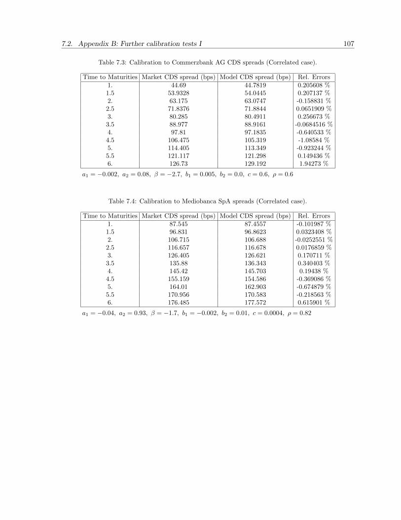
7.2. Appendix B: Further calibration tests I 107
Table 7.3: Calibration to Commerzbank AG CDS spreads (Correlated case).
Time to Maturities Market CDS spread (bps) Model CDS spread (bps) Rel. Errors1. 44.69 44.7819 0.205608 %1.5 53.9328 54.0445 0.207137 %2. 63.175 63.0747 -0.158831 %2.5 71.8376 71.8844 0.0651909 %3. 80.285 80.4911 0.256673 %3.5 88.977 88.9161 -0.0684516 %4. 97.81 97.1835 -0.640533 %4.5 106.475 105.319 -1.08584 %5. 114.405 113.349 -0.923244 %5.5 121.117 121.298 0.149436 %6. 126.73 129.192 1.94273 %
a1 = −0.002, a2 = 0.08, β = −2.7, b1 = 0.005, b2 = 0.0, c = 0.6, ρ = 0.6
Table 7.4: Calibration to Mediobanca SpA spreads (Correlated case).
Time to Maturities Market CDS spread (bps) Model CDS spread (bps) Rel. Errors1. 87.545 87.4557 -0.101987 %1.5 96.831 96.8623 0.0323408 %2. 106.715 106.688 -0.0252551 %2.5 116.657 116.678 0.0176859 %3. 126.405 126.621 0.170711 %3.5 135.88 136.343 0.340403 %4. 145.42 145.703 0.19438 %4.5 155.159 154.586 -0.369086 %5. 164.01 162.903 -0.674879 %5.5 170.956 170.583 -0.218563 %6. 176.485 177.572 0.615901 %
a1 = −0.04, a2 = 0.93, β = −1.7, b1 = −0.002, b2 = 0.01, c = 0.0004, ρ = 0.82

108 Chapter 7. Appendix
Table 7.5: Calibration to Deutsche Bank AG spreads (Correlated case).
Time to Maturities Market CDS spread (bps) Model CDS spread (bps) Rel. Errors1. 67.02 66.42 -0.895209 %1.5 77.7864 79.1848 1.79767 %2. 92.015 92.5289 0.558545 %2.5 107.233 105.796 -1.33972 %3. 120.505 118.488 -1.67348 %3.5 129.985 130.235 0.192996 %4. 138.645 140.774 1.53567 %4.5 149.244 149.928 0.458061 %5. 158.86 157.592 -0.798277 %5.5 164.376 163.718 -0.400654 %6. 167.59 168.305 0.426501 %
a1 = −0.1, a2 = 1.55, β = −0.08, b1 = −0.001, b2 = 0.006, c = 0.0003, ρ = 0.83
In tables— , in compute the survival probabilities for each CDS and we compare them to those obtained
by bootstrapping and used in the real market. One can see that our model give a very good fit to the
real market data and with the calibrated parameters one obtains survival probabilities close to the real
market ones.
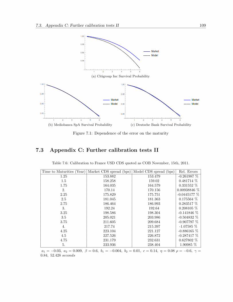
7.3. Appendix C: Further calibration tests II 109
(a) Citigroup Inc Survival Probability
(b) Mediobanca SpA Survival Probability (c) Deutsche Bank Survival Probability
Figure 7.1: Dependence of the error on the maturity
7.3 Appendix C: Further calibration tests II
Table 7.6: Calibration to France USD CDS quoted as COB November, 15th, 2011.
Time to Maturities (Year) Market CDS spread (bps) Model CDS spread (bps) Rel. Errors1.25 153.882 153.479 -0.261987 %1.5 158.258 159.02 0.481714 %1.75 164.035 164.579 0.331552 %2. 170.14 170.156 0.00938846 %
2.25 175.829 175.751 -0.0445177 %2.5 181.045 181.363 0.175564 %2.75 186.464 186.993 0.283517 %3. 192.24 192.64 0.208105 %
3.25 198.586 198.304 -0.141846 %3.5 205.021 203.986 -0.504832 %3.75 211.605 209.684 -0.907797 %4. 217.74 215.397 -1.07585 %
4.25 223.104 221.127 -0.886165 %4.5 227.526 226.872 -0.287417 %4.75 231.179 232.631 0.627802 %5. 233.936 238.404 1.90985 %
a1 = −0.03, a2 = 0.009, β = 0.6, b1 = −0.004, b2 = 0.01, c = 0.14, η = 0.08 ρ = −0.6, γ =0.84, 52.428 seconds
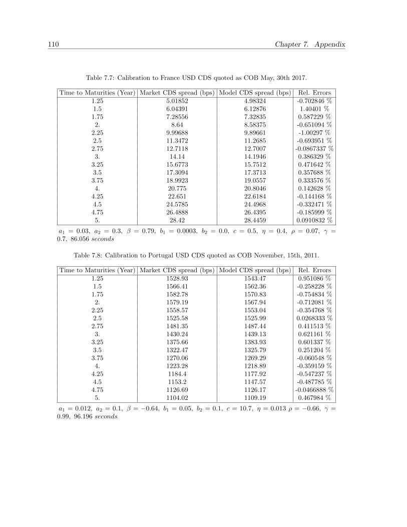
110 Chapter 7. Appendix
Table 7.7: Calibration to France USD CDS quoted as COB May, 30th 2017.
Time to Maturities (Year) Market CDS spread (bps) Model CDS spread (bps) Rel. Errors1.25 5.01852 4.98324 -0.702846 %1.5 6.04391 6.12876 1.40401 %1.75 7.28556 7.32835 0.587229 %2. 8.64 8.58375 -0.651094 %
2.25 9.99688 9.89661 -1.00297 %2.5 11.3472 11.2685 -0.693951 %2.75 12.7118 12.7007 -0.0867337 %3. 14.14 14.1946 0.386329 %
3.25 15.6773 15.7512 0.471642 %3.5 17.3094 17.3713 0.357688 %3.75 18.9923 19.0557 0.333576 %4. 20.775 20.8046 0.142628 %
4.25 22.651 22.6184 -0.144168 %4.5 24.5785 24.4968 -0.332471 %4.75 26.4888 26.4395 -0.185999 %5. 28.42 28.4459 0.0910832 %
a1 = 0.03, a2 = 0.3, β = 0.79, b1 = 0.0003, b2 = 0.0, c = 0.5, η = 0.4, ρ = 0.07, γ =0.7, 86.056 seconds
Table 7.8: Calibration to Portugal USD CDS quoted as COB November, 15th, 2011.
Time to Maturities (Year) Market CDS spread (bps) Model CDS spread (bps) Rel. Errors1.25 1528.93 1543.47 0.951086 %1.5 1566.41 1562.36 -0.258228 %1.75 1582.78 1570.83 -0.754834 %2. 1579.19 1567.94 -0.712081 %
2.25 1558.57 1553.04 -0.354768 %2.5 1525.58 1525.99 0.0268333 %2.75 1481.35 1487.44 0.411513 %3. 1430.24 1439.13 0.621161 %
3.25 1375.66 1383.93 0.601337 %3.5 1322.47 1325.79 0.251204 %3.75 1270.06 1269.29 -0.060548 %4. 1223.28 1218.89 -0.359159 %
4.25 1184.4 1177.92 -0.547237 %4.5 1153.2 1147.57 -0.487785 %4.75 1126.69 1126.17 -0.0466888 %5. 1104.02 1109.19 0.467984 %
a1 = 0.012, a2 = 0.1, β = −0.64, b1 = 0.05, b2 = 0.1, c = 10.7, η = 0.013 ρ = −0.66, γ =0.99, 96.196 seconds

7.3. Appendix C: Further calibration tests II 111
Table 7.9: Calibration to Portugal USD CDS quoted as COB May, 30th 2017.
Time to Maturities (Year) Market CDS spread (bps) Model CDS spread (bps) Rel. Errors1.25 55.7676 56.6391 1.56276 %1.5 67.7586 68.2853 0.777373 %1.75 80.3718 79.9073 -0.57795 %2. 92.975 91.4484 -1.64194 %
2.25 104.727 102.853 -1.78851 %2.5 115.529 114.07 -1.2627 %2.75 125.543 125.049 -0.393047 %3. 135.15 135.747 0.441821 %
3.25 144.688 146.124 0.992659 %3.5 154.187 156.147 1.27133 %3.75 163.548 165.787 1.36936 %4. 173.19 175.025 1.05927 %
4.25 183.136 183.842 0.385523 %4.5 192.933 192.231 -0.364032 %4.75 201.949 200.186 -0.873256 %5. 210.07 207.707 -1.12481 %
a1 = 0.015, a2 = 0.5, β = 0.7, b1 = 0.0, b2 = 0.0, c = 0.53, η = 0.78, ρ = −0.65, γ =0.7, 79.192 seconds
Table 7.10: Calibration to Spain USD CDS quoted as COB November, 15th, 2011.
Time to Maturities (Year) Market CDS spread (bps) Model CDS spread (bps) Rel. Errors1.25 443.089 447.5 0.995382 %1.5 455.942 452.898 -0.667565 %1.75 461.191 457.574 -0.784297 %2. 462.81 461.585 -0.264677 %
2.25 464.557 464.99 0.0931244 %2.5 466.775 467.842 0.228544 %2.75 469.216 470.197 0.209013 %3. 471.4 472.106 0.149761 %
3.25 473.03 473.626 0.125969 %3.5 474.222 474.819 0.125775 %3.75 475.314 475.759 0.0935208 %4. 476.525 476.544 0.0040035 %
4.25 478.011 477.313 -0.146031 %4.5 479.465 478.267 -0.24985 %4.75 480.572 479.705 -0.180317 %5. 480.911 482.072 0.24148 %
a1 = −0.06, a2 = 0.44, β = 0.52, b1 = −0.002, b2 = 0.044, c = 0.4, η = 0.03 ρ = −0.6, γ =0.5, 58.548 seconds

112 Chapter 7. Appendix
Table 7.11: Calibration to Spain USD CDS quoted as COB May, 30th 2017.
Time to Maturities (Year) Market CDS spread (bps) Model CDS spread (bps) Rel. Errors1.25 33.5073 33.4062 -0.301704 %1.5 36.6139 36.5987 -0.0413123 %1.75 39.678 39.7374 0.149748 %2. 42.74 42.8222 0.192309 %
2.25 45.7535 45.8532 0.218024 %2.5 48.7076 48.8305 0.252401 %2.75 51.6109 51.7541 0.277466 %3. 54.535 54.624 0.163207 %
3.25 57.5301 57.4403 -0.156104 %3.5 60.4933 60.2031 -0.479832 %3.75 63.2717 62.9123 -0.56793 %4. 65.87 65.5682 -0.458181 %
4.25 68.2415 68.1708 -0.103697 %4.5 70.5227 70.7201 0.279874 %4.75 72.8767 73.2164 0.466098 %5. 75.59 75.6597 0.0922325 %
a1 = −0.014, a2 = 0.073, β = 0.62, b1 = 0.002, b2 = 0.001, c = 0.28, η = 0.6, ρ = −0.38, γ =0.96, 63.304 seconds

Bibliography
[1] M. T. Barlow. Study of a filtration expanded to include an honest time. Zeitschrift fur Wahrschein-
lichkeitstheorie und Verwandte Gebiete, 44(4):307–323, Dec 1978.
[2] A. Bermudez, M. Nogueiras, and C. Vazquez. Numerical analysis of convection-diffusion-reaction
problems with higher order characteristics/finite elements. part ii: Fully discretized scheme and
quadrature formulas. SIAM Journal on Numerical Analysis, 44(5):1854–1876, 2006.
[3] A. Bermudez, M. Nogueiras, and C. Vazquez. Numerical analysis of convection-diffusion-reaction
problems with higher order characteristics/finite elements. part i: Time discretization. SIAM
Journal on Numerical Analysis, 44(5):1829–1853, 2006.
[4] F. Black and J. C. Cox. Valuing corporate securities: Some effects of bond indenture provisions.
Journal of Finance, 31(2):351–67, 1976.
[5] D. Brigo and A. Alfonsi. Credit default swap calibration and derivatives pricing with the ssrd
stochastic intensity model. Finance and Stochastics, 9(1):29–42, Jan 2005.
[6] D. Brigo and F. Mercurio. Interest Rate Models — Theory and Practice: With Smile, Inflation and
Credit. Springer Finance. Springer, 2 edition, Jan 2006.
[7] D. Brigo, N. Pede, and A. Petrelli. Multi currency credit default swaps: Quanto effects and fx
devaluation jumps. Dec 2015.
[8] M. C. Calvo-Garrido and C. Vazquez. Pricing pension plans based on average salary without early
retirement: Pde modeling and numerical solution. Journal of Computational Finance, 16:101–140,
2012.
113

114 BIBLIOGRAPHY
[9] P. Carr and V. Linetsky. A jump to default extended CEV model: an application of Bessel processes.
Finance Stoch., 10(3):303–330, 2006.
[10] D. Duffie, M. Schroder, and C. Skiadas. Recursive valuation of defaultable securities and the timing
of resolution of uncertainty. Ann. Appl. Probab., 6(4):1075–1090, 11 1996.
[11] D. Duffie and K. Singleton. Modeling term structures of defaultable bonds. Review of Financial
Studies, 12(4):687–720, 1999.
[12] P. Ehlers and P. Schonbucher. The influence of fx risk on credit spreads. 04 2004.
[13] G. Fichera. On a unified theory of boundary value problems for elliptic-parabolic equations of
second order in boundary value problems. SIAM Journal on Applied Mathematics, 73(5):1747–1767,
2013.
[14] J. Gatheral, E. P. Hsu, P. Laurence, C. Ouyang, and T.-H. Wang. Asymptotics of implied volatility
in local volatility models. Math. Finance, 22(4):591–620, 2012.
[15] R. Geske. The valuation of corporate liabilities as compound options. The Journal of Financial
and Quantitative Analysis, 12(4):541–552, 1977.
[16] K. Ito. Extension of stochastic integral. Proceedings of the International Symposium on Stochastic
Differential Equation, pages 95–109, 1978.
[17] R. Jarrow and S. Turnbull. Credit risk: Drawing the analogy. Risk Magazine, 5(9), 1992.
[18] R. Jarrow and S. M. Turnbull. Pricing derivatives on financial securities subject to credit risk.
Journal of Finance, 50(1):53–85, 1995.
[19] M. Jeanblanc and M. Rutkowski. Default risk and hazard process. In Mathematical finance—
Bachelier Congress, 2000 (Paris), Springer Finance, pages 281–312. Springer, Berlin, 2002.
[20] M. Jeanblanc, M. Yor, and M. Chesney. Mathematical methods for financial markets. Springer
Finance. Springer-Verlag London, Ltd., London, 2009.
[21] M. Jeanblanc, M. Yor, and M. Chesney. Mathematical Methods for Financial Markets, volume 31.
2010.
[22] Y.-M. Jeulin, Thierry. Grossissement d’une filtration et semi-martingales : formules explicites.
Seminaire de probabilites de Strasbourg, 12:78–97, 1978.
BIBLIOGRAPHY 115
[23] Y. Jiao and S. Li. Modelling sovereign risks: from a hybrid model to the generalized density
approach. working paper or preprint, May 2015.
[24] I. Karatzas and S. E. Shreve. Brownian motion and stochastic calculus. May 2018.
[25] I. J. Kim, K. Ramaswamy, and S. Sundaresan. Does default risk in coupons affect the valuation of
corporate bonds? : A contingent claims model. 22, Fev 1993.
[26] P. Kovalov and V. Linetsky. Valuing convertible bonds with stock price, volatility, interest rate,
and default risk. Jan 2008.
[27] A. Lanconelli, S. Pagliarani, and A. Pascucci. Local densities for a class of degenerate diffusions.
Mar 2018.
[28] F. A. Longstaff and E. S. Schwartz. A simple approach to valuing risky fixed and floating rate debt.
The Journal of Finance, 50(3):789–819, 1995.
[29] M. Lorig, S. Pagliarani, and A. Pascucci. Analytical expansions for parabolic equations. SIAM J.
Appl. Math., 75(2):468–491, 2015.
[30] A. P. M. C. Calvo-Garrido and C. Vazquez. Mathematical analysis and numerical methods for pricing
pension plans allowing early retirement. SIAM Journal on Applied Mathematics, 73(5):1747–1767,
2013.
[31] D. B. Mandan and H. Unal. Pricing the risks of default. Review of Derivatives Research, pages
121–160, 1999.
[32] R. Mendoza-Arriaga, P. Carr, and V. Linetsky. Time-changed Markov processes in unified credit-
equity modeling. Math. Finance, 20(4):527–569, 2010.
[33] R. Mendoza-Arriaga and V. Linetsky. Pricing equity default swaps under the jump-to-default
extended cev model. Finance and Stochastics, 15(3):513–540, Sep 2011.
[34] R. C. Merton. On the pricing of corporate debt: The risk structure of interest rates. The Journal
of Finance, 29(2):449–470, 1974.
[35] Moody’s Global Credit Research. Sovereign - global: Sovereign default and recovery rates, 1983-2015.
June 2016.
116 BIBLIOGRAPHY
[36] O. A. Oleinik and E. V. Radkevic. Second order equations with nonnegative characteristic form.
American Mathematical Society, 1973.
[37] S. Pagliarani and A. Pascucci. Asymptotic expansions for degenerate parabolic equations. C. R.
Math. Acad. Sci. Paris, 352(12):1011–1016, 2014.
[38] S. Pagliarani and A. Pascucci. The exact Taylor formula of the implied volatility. Finance Stoch.,
21(3):661–718, 2017.
[39] A. Pascucci. PDE and martingale methods in option pricing, volume 2 of Bocconi & Springer Series.
Springer, Milan; Bocconi University Press, Milan, 2011.
[40] K. Ramaswamy and S. M. Sundaresan. The valuation of floating-rate instruments: Theory and
evidence. Journal of Financial Economics, 17(2):251 – 272, 1986.
[41] C. Zhou, M. Pritsker, K. Ramaswamy, and R. Stulz. A jump-diffusion approach to modeling credit
risk and valuing defaultable securities. Jul 2004.