crude oil scheduling in refinery operations
TRANSCRIPT
CRUDE OIL SCHEDULING IN REFINERY OPERATIONS
P.CHANDRA PRAKASH REDDY
NATIONAL UNIVERSITY OF SINGAPORE
2003
CRUDE OIL SCHEDULING IN REFINERY OPERATIONS
P.CHANDRA PRAKASH REDDY ( B. Tech. OSMANIA, HYDERABAD)
A THESIS SUBMITTED FOR THE DEGREE OF
MASTER OF ENGINEERING
DEPARTMENT OF CHEMICAL & ENVIRONMENTAL ENGINEERING
NATIONAL UNIVERSITY OF SINGAPORE
2003

Name : Prodduturi ChandraPrakash Reddy Degree : M.Eng Department : Chemical and Environmental Engineering Title : Crude Oil Scheduling in Refinery Operations
ABSTRACT
Scheduling is one of the tools that facilitates refiner to be proactive for changing scenarios
and allows finding solutions that generate enhanced income. Scheduling considerations
prevalent with crude oil operations in a petroleum refinery have been addressed in this
work. Scheduling of crude oil operations is part of optimization of overall refinery
operations and involves unloading crude oil from vessels to storage tanks and charging
various mixes of crude oils from tanks to each distillation unit subject to capacity, flow,
and composition limitations. Refinery configurations with different unloading facilities
such as SBM (Single Buoy Mooring), multiple jetties are considered in this study.
Scheduling of crude oil operations is a complex nonlinear problem, especially when tanks
hold crude mixes. A novel iterative MILP solution approach for optimizing crude oil
operations is devised which obviates the need for solving MINLP. This work addresses
both discrete and continuous time scheduling models for crude oil scheduling problem and
presents a head to head comparison of the two models. The proposed methodology
performs much better in comparison to methodologies present in the literature and gives
near optimum solutions, thus making them suitable for large-scale operations.
Keywords: scheduling, crude oil, petroleum refinery, Single Buoy Mooring (SBM),
multiple jetties, MILP, MINLP.

ACKNOWLEDGEMENTS
I am very happy to take this opportunity to thank Dr. I. A. Karimi and Dr. R.
Srinivasan for their invaluable guidance, thought sharing and suggestions throughout
my research period at National University of Singapore, Singapore. Their ideas and
recommendations on the project have played a significant role in completing this work
successfully. Further, I extend my sincere and deepest gratitude for their priceless
advice, motivation and moral support throughout my stay here in Singapore.
I would like to thank all my friends and colleagues who helped me in one way or other
to carry out the research work successfully. In particular, I wish to thank Mr. Sushant
Gupta, Mr. Swarnendu Bhushan, Mr. Tian Wende and Mr. Prabhat Agrawal for
actively participating in the discussion related to my project work. I am very thankful
to my wife, children, and parents for their moral support, love and needless to mention,
I am thankful to God, the eternal guide, for his love and blessings.
Finally, I would like to thank the National University of Singapore for providing the
research scholarship to complete this project.
i
TABLE OF CONTENTS
ACKNOWLEDGEMENTS i
SUMMARY vii
NOMENCLATURE ix
LIST OF FIGURES xv
LIST OF TABLES xvi
1. INTRODUCTION 1
1.1 Introduction to Refining Industry 1
1.2 Need For Scheduling 3
1.3 Terminology 5
1.4 Scheduling Considerations 6
1.4.1 Planning Objectives 9
1.4.2 Scheduling Objectives 9
1.4.3 Processing Constraints 10
1.4.4 Uncertainties 10
1.5 Anticipated Benefits 11
1.6 Research Objective 12
1.7 Outline Of The Thesis 13
2. LITERATURE SURVEY 14
2.1 Planning and Scheduling in Petroleum Refinery 17
2.2 Recent Work 20
2.3 Crude Oil Scheduling 24
2.4 Research Focus 29
ii
Table of Contents
3. PROBLEM DESCRIPTION 31
3.1 Introduction 31
3.2 Process Description 32
3.2.1 Problem Statement 34
3.2.2 Operating Rules 35
3.2.3 Assumptions 35
3.3 Motivating Examples 36
3.3.1 Example 1 37
3.3.2 Example 2 40
3.3.3 Example 3 43
3.4 Outline 45
4. MODEL FORMULATION - Discrete Time (part I) 46
4.1 Time Representation 46
4.2 Unloading Via SBM 47
4.2.1 Parcel Creation 47
4.2.2 Parcel-to-SBM Connections 49
4.2.3 Parcel-to-Tank Connections 50
4.2.4 SBM-to-Tank Connections 51
4.2.5 Crude Delivery and Processing 52
4.2.6 Crude Inventory 54
4.2.7 Production Requirements 55
4.2.8 Scheduling Objective 56
4.3 Unloading Via Jetties 58
iii

Table of Contents
4.4 Unloading Via SBM and Jetties 59
4.5 Tank-to-Tank Transfers 60
5. SOLUTION ALGORITHM - Discrete Time 65
5.1 Description 65
5.2 Stepwise Methodology 66
5.3 Illustration 69
5.4 Remarks 71
6. MODEL EVALUATION 74
6.1 Examples 74
6.1.1 Data Tables 75
6.1.1.1 Example 1 75
6.1.1.2 Examples 2-6 76
6.1.2 Results and Discussion 78
6.1.2.1 Example 1 78
6.1.2.2 Example 2 81
6.1.2.3 Example 3 84
6.1.2.4 Example 4 84
6.1.2.5 Example 5 88
6.1.2.6 Example 6 88
6.2 Conclusion 91
7. MODEL FORMULATION - Continuous Time (part II) 92
7.1 Introduction 92
7.2 Refinery Configuration 95
7.3 MILP Formulation 95
7.3.1 Time Representation 95
iv
Table of Contents
7.3.2 Parcel Creation 97
7.3.3 Parcel-to-SBM Connections 97
7.3.4 SBM-to-Tank Connections 98
7.3.5 Tank-to-CDU Connections 98
7.3.6 Tank Activity 99
7.3.7 Activity Durations 100
7.3.8 Crude Unloading 102
7.3.9 Crude Processing 102
7.3.10 Crude Balance 103
7.3.11 Brine Settling 104
7.3.12 Changeovers 105
7.3.13 Crude Demand 105
7.3.14 Demurrage 105
7.3.15 Objective 106
8. SOLUTION ALGORITHM-Continuous Time 108
8.1 Introduction 108
8.2 Description 108
8.3 Step-wise Procedure 109
8.4 Discussion 110
9. COMPUTATIONAL RESULTS 112
9.1 Examples 112
9.2 Example 1 118
9.3 Example 2 121
9.4 Example 3 122
9.5 Conclusion 125
v

Table of Contents
10. CONCLUSIONS AND RECOMMENDATIONS 126
10.1 Conclusions 126
10.2 Recommendations 127
REFERENCES 129
APPENDIX A
A.1: GAMS file - case-1 discrete time model for example-1 of part II 136
A.2: GAMS file - continuous time model for example-1 of part II 152
vi

SUMMARY
Scheduling considerations prevalent with crude oil operations in a petroleum refinery
have been addressed in this work. Scheduling of crude oil operations involves
unloading crude oil from vessels to storage tanks and charging various mixes of crude
oils from tanks to each distillation unit subject to capacity, flow, and composition
limitations. Refinery configurations with different unloading facilities such as SBM
(Single Buoy Mooring), multiple jetties are considered in this study. Time
consideration in model building is very important. Two different methodologies are
adopted namely discrete time, continuous time. Firstly a discrete time MILP (mixed
integer linear programming) model is formulated for a refinery configuration with
SBM, storage tanks and crude distillation units. The objective is to maximize the gross
operating profit. The model is extended to a refinery with multiple jetties alone as
crude unloading facility and then to a refinery configuration with jetties along with
SBM. A separate MILP model is developed in case of a refinery configuration which
includes both SBM, jetties as unloading facility, storage tanks for crude receipt from
vessels and crude delivery to distillation units. Mimicking a continuous-time
formulation, the developed model allows multiple sequential crude transfers to occur
within a time slot. Furthermore, it handles many real-life operational features including
brine settling and tank-to-tank transfers.
Scheduling of crude oil operations is a complex nonlinear problem, especially when
tanks hold crude mixes. Crude mixing generates in bi-linear non-convex equations,
which are hard to solve, and the problem is a MINLP. A linearized model poses
composition discrepancy in crude charge to CDU. A novel iterative solution approach
vii

Summary
for optimizing crude oil operations is devised which corrects the concentration
discrepancy arising due to crude mixing in tanks without solving any NLP or MINLP.
The size and complexity of MILP in proposed algorithm reduce progressively
and provides near-optimal schedules in reasonable time. When the scheduling
objective does not involve crude compositions, then proposed algorithm guarantees a
globally optimal objective value right in the first MILP, although subsequent iterations
are required to correct the composition discrepancy. Both these proposed model and
algorithms perform much better in comparison to scheduling methodologies present in
the literature and give better solutions for several literature problems, thus making
them suitable for large-scale operations. The test examples are solved for a short term
scheduling horizon and conclusions are made regarding the system in general.
The second part addresses a continuous time mathematical model for a refinery
configuration with SBM. The model is based on synchronized variable length slots on
storage tanks. Here an attempt was made to reduce number of binary decisions so that
model becomes less compute intensive. For solving the continuous model that provides
schedules with no composition discrepancy, we incorporated suitable modifications to
the solution algorithm of discrete approach. A direct comparison of discrete and
continuous models is carried out and it was concluded that for long horizons
continuous time model generates a feasible schedule in reasonable time. For shorter
horizons, discrete time models provided a better and quicker solution, thus having an
edge over the continuous time models.
Finally the thesis is concluded with a summary of prominent improvements
achieved in comparison to previous works and some future directions are proposed.
viii
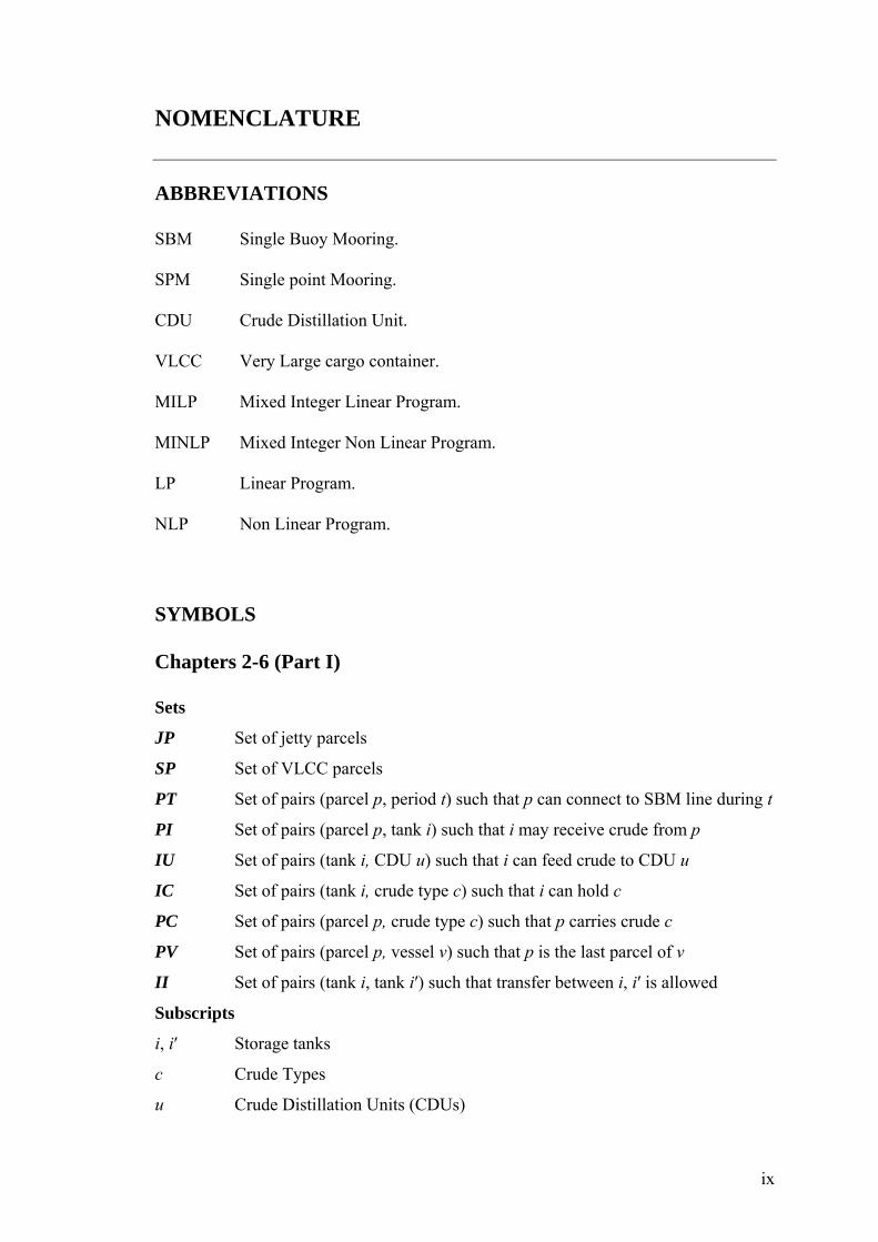
NOMENCLATURE
ABBREVIATIONS
SBM Single Buoy Mooring.
SPM Single point Mooring.
CDU Crude Distillation Unit.
VLCC Very Large cargo container.
MILP Mixed Integer Linear Program.
MINLP Mixed Integer Non Linear Program.
LP Linear Program.
NLP Non Linear Program.
SYMBOLS
Chapters 2-6 (Part I)
Sets
JP Set of jetty parcels
SP Set of VLCC parcels
PT Set of pairs (parcel p, period t) such that p can connect to SBM line during t
PI Set of pairs (parcel p, tank i) such that i may receive crude from p
IU Set of pairs (tank i, CDU u) such that i can feed crude to CDU u
IC Set of pairs (tank i, crude type c) such that i can hold c
PC Set of pairs (parcel p, crude type c) such that p carries crude c
PV Set of pairs (parcel p, vessel v) such that p is the last parcel of v
II Set of pairs (tank i, tank i′) such that transfer between i, i′ is allowed
Subscripts
i, i′ Storage tanks
c Crude Types
u Crude Distillation Units (CDUs)
ix

Nomenclature
v Vessels
t Time periods
p Parcels
Superscripts
U Upper limit
L Lower limit
Parameters
ETAp Expected time of arrival of parcel p L / UpiFPT Limits on the amount of crude transfer per period from parcel p to tank i
L / UiuFTU Limits on the amount of crude charge per period from tank i to CDU u
L / UiiFTT ′ Limits on the amount of crude transfer per period from tank i to i’
L / UuFU Limits on the amount of crude processed per period by CDU u
L / Ucuxc Limits on the composition of crude type c in feed to CDU u
L / Ukuxk Limits on the concentration of key component k in feed to CDU u
L / UiV Allowable limits on crude inventory in tank i
L / Uicxt Limits on the composition of crude type c in tank i
D Total crude demand in the scheduling horizon
uD Total crude demand per CDU u in the scheduling horizon
utD Crude demand per CDU u in each period t
jPD Maximum demand for product j during scheduling horizon
jcuy Fractional yield of product j from crude c in CDU u
cuCP Margin ($/unit volume) for crude c in CDU u
COC Cost (k$) per changeover
TTC Penalty (K$) for occurrence of a tank-to-tank transfer
SSP Safety stock penalty ($ per unit volume below desired safety stock)
SS Desired safety stock (kbbl) of crude inventory in any period
SWCv Demurrage or Sea waiting cost ($ per period)
ETDv Expected time of departure of vessel v
ETUp Earliest possible unloading period for parcel p
PSp Size of the parcel p
J Number of identical Jetties
x

Nomenclature
Binary Variables
XPpt 1 if parcel p is connected to SBM/jetty discharge line during period t
XTit 1 if a tank i is connected to SBM/jetty discharge line during period t
Yiut 1 if a tank i feeds CDU u during period t
Zii′t 1 if crude transfers between tanks i and i′ during period t
0-1 Continuous Variables
XFpt 1 if a parcel p first connects to the SBM/jetty during period t
XLpt 1 if a parcel p disconnects from the SBM/jetty at time t
Xpit 1 if a parcel p and tank i both connect to the SBM line at t
YYiut 1 if a tank i is connected to CDU u during both periods t and (t+1)
COut 1 if a CDU u has a changeover during period t
Continuous Variables
TFp Time at which parcel p first connects to SBM/jetty for unloading
TLp Time at which parcel p disconnects from SBM/jetty after unloading
FPTpit Amount of crude transferred from parcel p to tank i during period t
FTUiut Amount of crude that tank i feeds to CDU u during period t
FUut Total amount of crude fed to CDU u during period t
FCTUiuct The amount of crude c delivered by tank i to CDU u during period t
VCTict Amount of crude c in tank i at the end of period t
Vit Crude level in tank i at end of period t
fict Concentration (volume fraction) of crude c in tank i at the end of period t
DCv Demurrage cost for vessel v
SCt Safety stock penalty for period t
ZTit Variable to denote the number of times tank i exchanges crude with
another tank in a given period t
ii ctFCTT ′ The amount of crude c transferred from tank i to tank i′ during period t
ii tFTT ′ Total amount of crude transferred between tank i to tank i′during t
ii tAFTT ′ Absolute amount of crude transferred between tank i to tank i′ during t
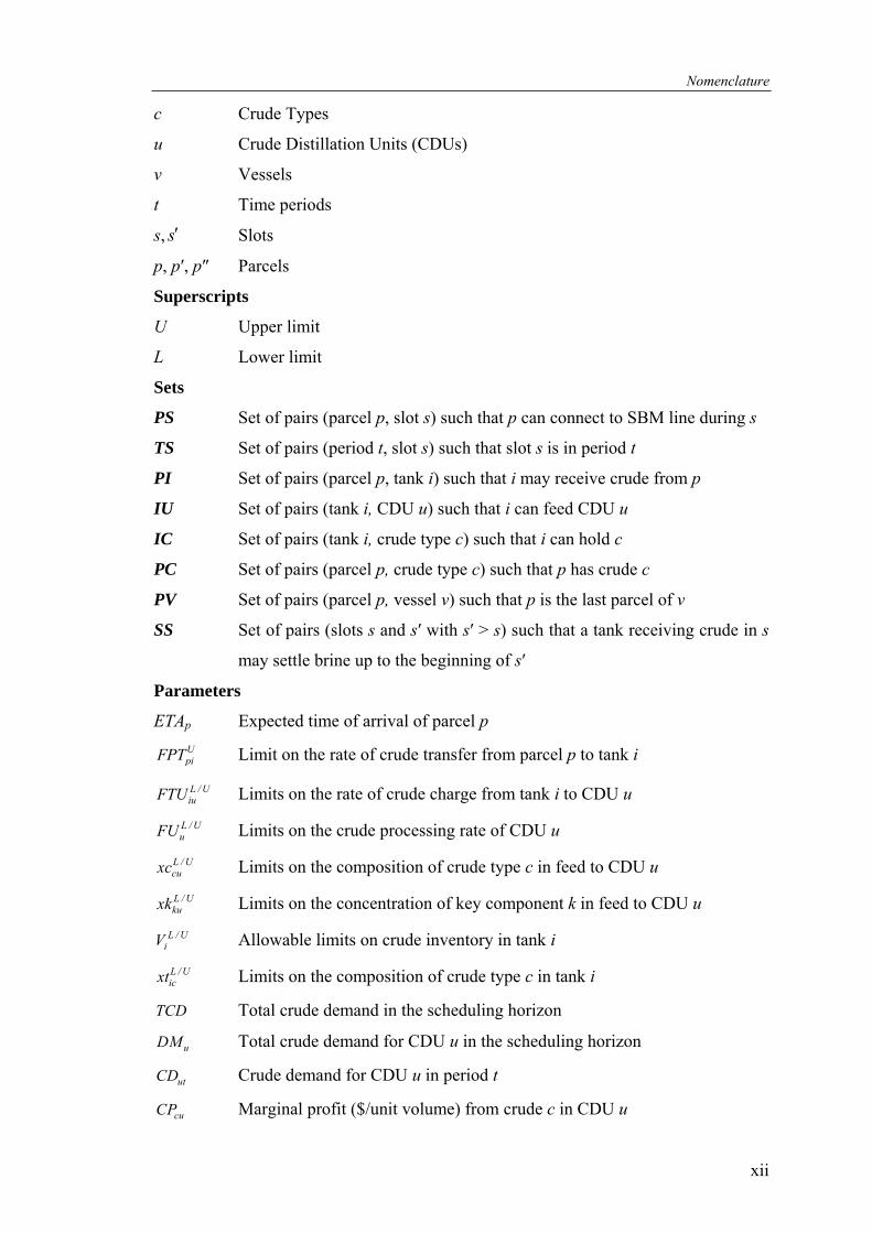
Chapters 7-9 (Part II)
Subscripts
i Storage tanks
xi
Nomenclature
c Crude Types
u Crude Distillation Units (CDUs)
v Vessels
t Time periods
s, Slots s′
p, p′, p″ Parcels
Superscripts
U Upper limit
L Lower limit
Sets
PS Set of pairs (parcel p, slot s) such that p can connect to SBM line during s
TS Set of pairs (period t, slot s) such that slot s is in period t
PI Set of pairs (parcel p, tank i) such that i may receive crude from p
IU Set of pairs (tank i, CDU u) such that i can feed CDU u
IC Set of pairs (tank i, crude type c) such that i can hold c
PC Set of pairs (parcel p, crude type c) such that p has crude c
PV Set of pairs (parcel p, vessel v) such that p is the last parcel of v
SS Set of pairs (slots s and s′ with s′ > s) such that a tank receiving crude in s
may settle brine up to the beginning of s′
Parameters
ETAp Expected time of arrival of parcel p UpiFPT Limit on the rate of crude transfer from parcel p to tank i
L / UiuFTU Limits on the rate of crude charge from tank i to CDU u
L / UuFU Limits on the crude processing rate of CDU u
L / Ucuxc Limits on the composition of crude type c in feed to CDU u
L / Ukuxk Limits on the concentration of key component k in feed to CDU u
L / UiV Allowable limits on crude inventory in tank i
L / Uicxt Limits on the composition of crude type c in tank i
TCD Total crude demand in the scheduling horizon
uDM Total crude demand for CDU u in the scheduling horizon
utCD Crude demand for CDU u in period t
cuCP Marginal profit ($/unit volume) from crude c in CDU u
xii
Nomenclature
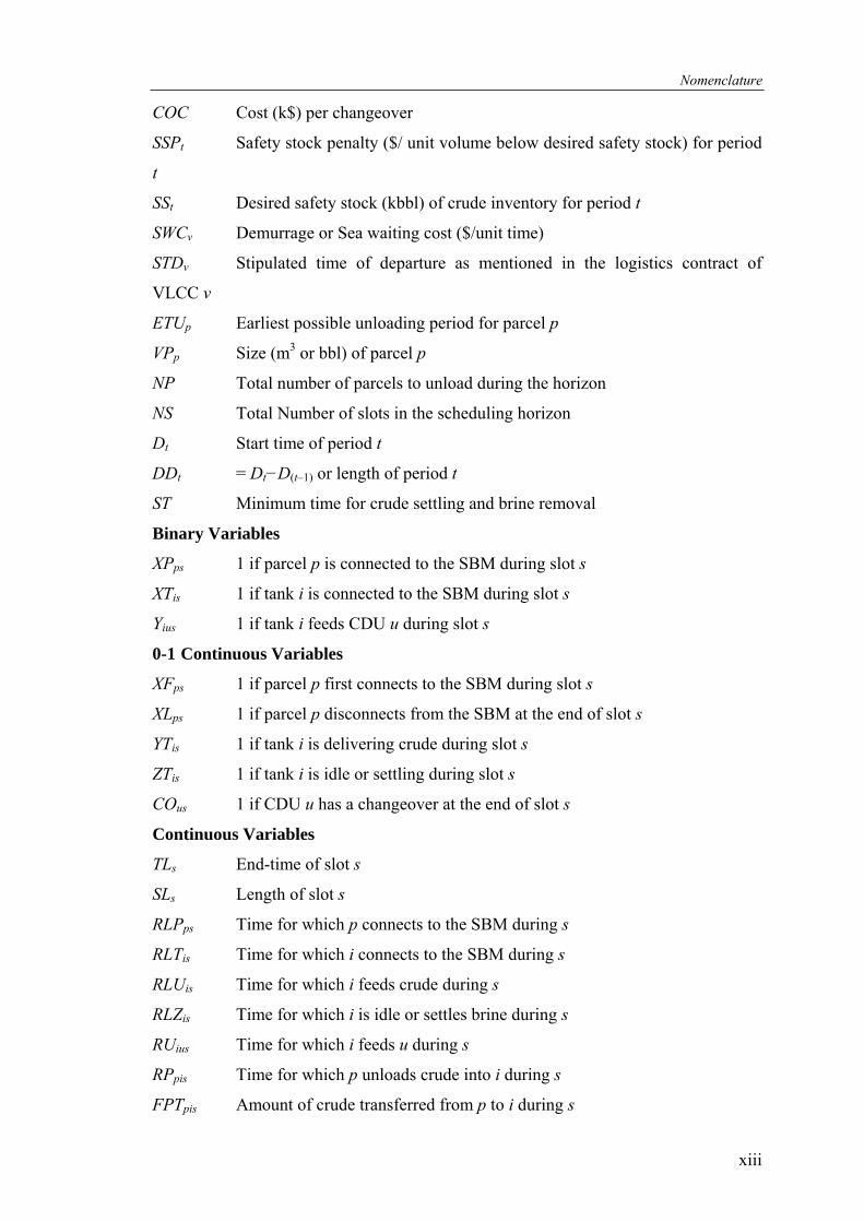
COC Cost (k$) per changeover
SSPt Safety stock penalty ($/ unit volume below desired safety stock) for period
t
SSt Desired safety stock (kbbl) of crude inventory for period t
SWCv Demurrage or Sea waiting cost ($/unit time)
STDv Stipulated time of departure as mentioned in the logistics contract of
VLCC v
ETUp Earliest possible unloading period for parcel p
VPp Size (m3 or bbl) of parcel p
NP Total number of parcels to unload during the horizon
NS Total Number of slots in the scheduling horizon
Dt Start time of period t
DDt = Dt−D(t–1) or length of period t
ST Minimum time for crude settling and brine removal
Binary Variables
XPps 1 if parcel p is connected to the SBM during slot s
XTis 1 if tank i is connected to the SBM during slot s
Yius 1 if tank i feeds CDU u during slot s
0-1 Continuous Variables
XFps 1 if parcel p first connects to the SBM during slot s
XLps 1 if parcel p disconnects from the SBM at the end of slot s
YTis 1 if tank i is delivering crude during slot s
ZTis 1 if tank i is idle or settling during slot s
COus 1 if CDU u has a changeover at the end of slot s
Continuous Variables
TLs End-time of slot s
SLs Length of slot s
RLPps Time for which p connects to the SBM during s
RLTis Time for which i connects to the SBM during s
RLUis Time for which i feeds crude during s
RLZis Time for which i is idle or settles brine during s
RUius Time for which i feeds u during s
RPpis Time for which p unloads crude into i during s
FPTpis Amount of crude transferred from p to i during s
xiii

Nomenclature
FTUius Amount of crude that i feeds to u during s
FUus Total amount of crude feed to u during s
FCTUiucs Amount of c delivered by i to u during s
VCTics Amount of c in i at the end of s
Vis Crude level in i at the end of s
fics Concentration (volume fraction) of c in i at the end of s
DCv Demurrage for vessel v
SCt Safety stock penalty for period t
xiv

LIST OF FIGURES Figure 3.1 Schematic of oil unloading and processing
33
Figure 3.2 Operation schedule for the motivating example
37
Figure 3.3 Operation schedule for the motivating example of Lee et al. (1996)
40
Figure 4.1 Schematic representation of parcel creation
48
Figure 5.1
Flow chart for the solution algorithm
67
Figure 6.1
Key component concentration in CDU feeds at various time periods for example 2
83
Figure 7.1 Schematic of oil unloading using SBM and processing in CDUs
95
xv

LIST OF TABLES
Table 3.1 Candidate and optimal schedules for the motivating example
39
Table 3.2 Profit Comparison for candidate and optimal schedules
39
Table 3.3 Key component concentration in the feed to CDU for different allowable concentration limits (Cases 1 & 2) for charging tanks in Lee et al. (1996) motivating example and feed composition discrepancy in Case 2
42
Table 3.4 Charging schedule of CDUs obtained using Li et al. (2002) approach for the motivating example
44
Table 4.1 Constraints for different refinery configurations
62
Table 5.1 Details of individual iterations for the motivating example using the proposed algorithm
70
Table 6.1 Crude arrival information for example 1
75
Table 6.2 Crude types and processing margin for example 1
75
Table 6.3 Initial crude inventory and storage capacities of storage tanks for example1
76
Table 6.4 Initial crude levels, capacities of storage tanks for examples 2-6
76
Table 6.5 Initial crude composition in storage tanks for examples 2-6
76
Table 6.6 Tanker arrival details, crude demands and key component concentration limits on CDUs for Examples 2 to 6
77
Table 6.7 Crude types, marginal profits and key component details for examples 2-6
78
Table 6.8 Economic data and limits on crude transfer amounts for examples 2-6
78
Table 6.9 Model performance and statistics for illustrated examples
79
Table 6.10 Operation schedule for Example 2 of Li et al (2002) obtained via our approach
80
Table 6.11 Jetty allocation Schedule for Example 2 of Li et al (2002) obtained via our approach
80
xvi
List of Tables
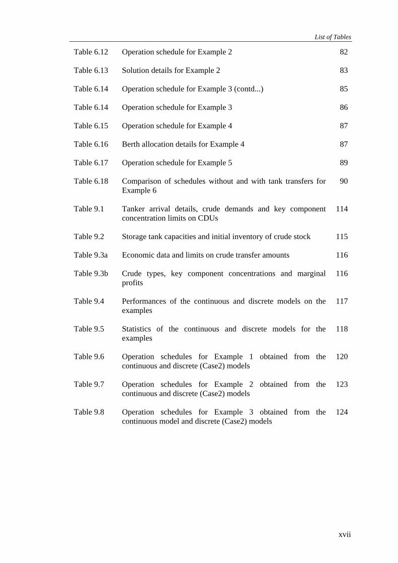
Table 6.12 Operation schedule for Example 2
82
Table 6.13 Solution details for Example 2
83
Table 6.14
Operation schedule for Example 3 (contd...)
85
Table 6.14 Operation schedule for Example 3
86
Table 6.15 Operation schedule for Example 4
87
Table 6.16 Berth allocation details for Example 4
87
Table 6.17 Operation schedule for Example 5
89
Table 6.18 Comparison of schedules without and with tank transfers for Example 6
90
Table 9.1 Tanker arrival details, crude demands and key component concentration limits on CDUs
114
Table 9.2 Storage tank capacities and initial inventory of crude stock
115
Table 9.3a Economic data and limits on crude transfer amounts
116
Table 9.3b Crude types, key component concentrations and marginal profits
116
Table 9.4 Performances of the continuous and discrete models on the examples
117
Table 9.5 Statistics of the continuous and discrete models for the examples
118
Table 9.6 Operation schedules for Example 1 obtained from the continuous and discrete (Case2) models
120
Table 9.7 Operation schedules for Example 2 obtained from the continuous and discrete (Case2) models
123
Table 9.8 Operation schedules for Example 3 obtained from the continuous model and discrete (Case2) models
124
xvii

Chapter 1
INTRODUCTION
1.1 Introduction to Refining industry
Petroleum is the second largest consumable on the planet, second only to water. The
modern society is dependent on petroleum products more than any other natural
resource for the comforts and convenience. The petroleum business involves many
independent operations, beginning with the search for oil and gas and extending to the
delivery of finished products, with incredibly complex manufacturing processes in the
middle. Each of these processes has unique objectives and demands. Unlike discrete
manufacturing, petroleum manufacturing does not start with bill of materials. A bill of
materials is a list of all the materials that go into making a particular product. In case
of petroleum processes feed stock and intermediates can come from a number of
different sources with significantly different qualities, and yet be processed and
combined to form precise products, meeting all regulatory specifications as well as
shipping times. Petroleum refining is a typical continuous process plant that has a
continuous flow of material going in and coming out. Crude oil is basic raw material
for producing most of petroleum products. Petroleum refining involves separating
crude oil into its constituents, purifying them, and converting them into marketable
products. In the refinery, crude enter the crude distillation unit and separated into
component streams. Some of these streams are desirable. The undesirable streams are
either subject to a series of treatments and undergo specific unit operations and
processes in separate units such as crackers, reformers and alkylation units to yield
desirable products or blended with desirable streams into finished products.
1
Chapter 1: Introduction
Undesirable streams may also be sold off or used as low-cost fuels. A general refinery
configuration includes crude handling facilities, distillation units, vacuum distillations
units, catalytic reforming units, fluid catalytic/Hydro cracking units, hydro treaters,
visbraker/delayed coker units and off-site storage/blending facilities to store/process
the finished products/intermediate streams. Distillation, vacuum distillation and
catalytic reforming units are normally grouped as primary processing units. Fluid
catalytic/hydro crackers, hydro treaters, visbraker/delayed coker units are grouped as
secondary units where heavier hydrocarbon streams are converted to more useful fuel
streams. Quality of the finished petroleum products is very important and has to be
strictly complied. Since crude is the basic raw material for producing these products,
quality of the crude oil is very crucial. Based on long range forecast of product
demand, crude oils are often planned, purchased, and have a delivery schedule set long
before they arrive at the refinery. In addition, crudes originated from different sources
have different qualities and product patterns, and even some times crudes from the
same origin differ in quality. So all the products cannot be produced from every type
of crude, and this difference in yield/quality poses different set of constraints on the
down stream treatment/processing units resulting in processing bottlenecks, lower
throughputs, excessive productions etc. Crude assay provides detailed yields/properties
of different cuts based on their boiling range. Impurities present in crudes limit their
processing to produce acceptable products. Impurities can be in the form of high sulfur
levels, higher metal content, higher levels of basic nitrogen or naphthenic acids etc.
Impure crudes are relatively cheaper but fewer refineries are equipped with the
required technology that allows processing these crudes. Capital investment in
acquiring, updating to the latest technologies is quite high and return on investment is
not very attractive. The operating conditions, processing requirements, available
2

Chapter 1: Introduction
technology, and production demands forces refiners to select such crudes which can be
processed neat or by blending among the available basket of crudes. Storage or
processing segregation of crude types is a common feature in refinery. Segregation is
based on key component levels, impurity levels in crudes and processability to yield
specific product pattern. Driven by market requirements, refinery operates in different
modes, each mode producing a different set of products. Sometimes the streams from
different modes are blended to meet product quality specification. Mode switch is
changing the feed to distillation unit from one type of crude segregation to other. Every
mode switch produces some off-spec production and needs reprocessing and mode
switches are inevitable in long run to meet demands. Normally refineries with multi
CDU configuration segregate processing and avoid mode switches unless inevitable.
Within segregated mode operation, change in feed composition to processing unit
results in perturbed operation in the unit resulting some production loss. Given a set of
crudes, considerable effort/expertise is required to identify better crude combinations
for processing in order to meet customer commitments and to boost gross profit
margins. Thus, the refining industry operates under uncertain product demand, and
uncertain manufacturing/plant capabilities leading to deviations in actual performance
to operating targets set by the monthly refinery plan.
1.2 Need for Scheduling
Every industrial manufacturing business aspires to have maximum profit/return on
investment. For being a market leader, the company needs to have a good global
coverage, efficient consumer services, lower production costs and reduced inventory
levels. Apart from these multiple objectives, the dynamic nature of demands and
uncertainties involved in a refinery makes the life of higher management more and
more difficult. The data flow into the system, in terms of sale targets/forecasts,
3
Chapter 1: Introduction
material/product inventories, manufacturing costs and deadlines (product delivery
dates, crude arrival time, etc), is also enormous. All these factors must be taken into
account for planning and scheduling of operations.
With a substantial increase in computational power of modern day computers,
there has been renewed interest in finding solutions to these planning/scheduling
problems keeping in view as many factors as possible. The next-generation decision
support systems, which employ Advanced Planning and Scheduling (APS) techniques,
coupled with supply chain management considerations have been in course of
development. With the advent of e-business age, when the dynamics of supply chains
and collaborations are redefining ways to conduct business, the core of success still
relies on seamless flow of information and material across various business ‘nodes’ in
‘networked’ economies. In such a high velocity environment, the goal is to optimize
the operations to have maximum gains and planning/scheduling forms the foundation
of this process.
In recent years, refining has become an extremely competitive business
characterized by fluctuating demands for products, ever-changing raw material prices,
and the incessant push towards cleaner fuels. To survive financially, a refinery must
operate efficiently. From an operational perspective, a plant would operate the best in a
steady state with consistent feed stocks and product requirement and all units operating
at full capacity. Any change is undesirable, as it may lead to off-spec products, reduced
throughputs, increased equipment wear and tear, uncertainty, and more work.
Nevertheless, in the current competitive environment, profit depends on agility, i.e.,
the ability to exploit short-term opportunities to fill demand at higher profit margins.
Processed crude compositions have the greatest influence on refinery margins.
4
Chapter 1: Introduction
Therefore, refiners tightly control the quality of crude charge and use advanced
technologies to plan and schedule crude oil changes.
The increasing reliance on petroleum products is motivation to find better ways
to process, and deliver products while maximizing the margins, minimizing the waste,
and improving the profitability within the constraints set by the nature of process and
environmental regulations. Managing the crude oil operations is vital for better
visibility of downstream processes. Since day-to-day operation enhancements are
precursors to high throughput and lower operating expenses of a refinery, the focus in
this work is on short-term scheduling of crude oil operations. By short term
scheduling, it is understood that monthly/weekly targets for the production facilities
are known a priori and the objective is to achieve the maximum from the system so as
to optimally utilize resources. Before the problem of scheduling is attempted, there is a
need for understanding the terminologies involved in refinery business and
requirements of a "good schedule".
1.3 Terminology
Crude handling facilities in refinery includes crude unloading facilities, storage
facilities and processing facilities. The raw material, crude is commonly transported
using sea route in small cargo ship called ‘crude tanker’ or ‘crude vessel’ that can
arrive near to the shore for mooring. The mooring station is called ‘Jetty’. Bearing in
mind the cost of transportation adding to the cost of raw material and looking at the
margins of processing, it is preferable to get different small crude packets normally
termed as ‘crude parcel’ in one VLCC (very large crude cargo) ship. VLCC cannot
come near to the shore requires special facility mooring called SBM (Single buoy
mooring). In both cases a pipeline connects the mooring station to the storage tanks at
refinery site. The pipeline connecting the SBM to refinery storage tanks is called
5

Chapter 1: Introduction
‘SBM line’. Crude is stored in floating roof tanks to avoid the vaporization losses.
Crude is normally pumped to a tank and pumped out of tank using different nozzles
connected at some height from the bottom of the tank and crude below this nozzle
height will be stagnant and is called ‘Heel’ of the tank. This portion facilitates the
sediments and brine to settle for periodic removal after every receipt of the crude. The
tank operation can be standing gauge or running gauge. Standing gauge operation
allows only one operation either receiving or delivering at any one point of time where
as running gauge allows both operations. Almost all tank operations in a refinery
follow standing gauge operation. ‘Demurrage’ or ‘sea waiting cost’ of a crude cargo
ship is the cost associated with delay in unloading crude from crude tanker beyond the
accepted time frame as per the logistic contract. A 'graph' , which provides all the
information of crude unloading amounts, parcel to tanks allocations, tank to processing
unit (CDUs) allocations and the amounts of crude processed that adequately define
production is termed as a 'schedule' and problem which yields this solution is the
scheduling problem. A schedule thus obtained can be feasible or infeasible. A 'feasible
schedule' is one that satisfies all possible constraints - material balances,
manufacturing, inventory, demand and user defined constraints. Such a schedule is
classified as 'optimum schedule' if it is rated as the best among all feasible schedules
based on the objectives - maximization of profits or minimization of production costs.
It is worthwhile to now focus on the issues to be addressed in developing optimum
schedules for scheduling of crude oil operations.
1.4 Scheduling Considerations
Planning and Scheduling primarily differ in terms of the time frames involved.
Planning is generally undertaken for longer time horizon (of the order of months and
years) and includes management objectives, policies, etc besides immediate processing
6

Chapter 1: Introduction
requirements. It represents aggregated objectives and usually does not include finer
details. Accordingly, the models used are either crude or take simplifying assumptions
making them more abstract. If the assumptions overestimate the facility performance
giving very little allowances, the resultant plan can become too ambitious and end up
as infeasible. On the other hand, if assumptions underestimate the plant's efficiency,
the plan thus obtained might be too conservative and lead to under-utilized production
capacities. Therefore, for planning operations, one must include the key detailed
constraints and their interdependencies in order to get an optimal plan and hence a
sound basis for undertaking further scheduling. On the other hand scheduling is the
link between the manufacturing process and the customer. The issues addressed by the
scheduling vary with the characteristics of the production process and the nature of
market served. A formal way of defining the scheduling is the specification of what at
each stage of production is supposed to do over short scheduling horizon ranging from
several shifts to week. This defines or projects the inputs to and outputs from each
production operation. Scheduling is the reality check on the planning process. The
objective of scheduling is implementation of the plan, subject to the variability that
occurs in the real world. This variability can be in feed stock supplies, quality, the
production process, customer requirements or the transport.
Optimization plays an important role in managing the oil refinery. Oil
refineries have used optimization techniques for a long time, specifically Linear
Programs (LPs) for the planning and scheduling of process operations. While the
planning systems provide coordination over several months, the scheduling systems
plan the activities over days to weeks. Planning precedes scheduling and uses
forecasted product demands. Scheduling includes plant level operations to realize the
plan. The refinery planning provides scheduling with volume-based information.
7

Chapter 1: Introduction
Planning determines the volumes of different feed stocks that will be consumed in
different modes. Planning does not provide timing of activities. The function of
scheduling group with in refinery is to define charge rates, and the timing of mode/tank
changes in response to product requirements and containment problems. A number of
refineries decompose the scheduling into crude scheduling, hydraulic scheduling, and
product scheduling. Crude schedulers react to the timing of crude arrivals, determine
which tank the crude should be placed in, blend crudes as needed to meet targets for
yields and qualities off the crude unit, and determine the charging rate to the crude
unit. Hydraulic scheduling is concerned with the operations on major units and
inventories between the units. The main objective is to have proper control on
intermediate inventories. Product scheduling is concerned with defining the timing of
blends and the activities required to move the products out of the refinery while
ensuring the inventory control.
Crudes are purchased based on the monthly refinery plan. Scheduling
subsequently accounts for deviations from the forecast and accounts for changes in
demand or plant capability. A priori information of the procured crudes including the
types, quantities, and expected times of arrival at the refinery, etc. is used to schedule
the short-term activities. These activities include (1) unloading crude oil from vessels
to storage tanks and (2) charging various mixes of crude oils to each distillation unit
subject to capacity, flow, and composition limitations. Scheduling of crude oil
operations defines the timing and the volumes of specific crude mix to be processed to
meet the demand while operating continuously with less containment problems.
8

Chapter 1: Introduction
1.4.1 Planning Objectives
Maximizing the gross refinery margin is the main objective of planning. Some of the
factors, which need to be taken into consideration at the highest level in the hierarchy
of planning, are:
1. Meeting demand forecast.
2. Efficient utilization of facility's resources (plant capacities, available
technology, utilities, manpower, etc).
3. Keeping low Work-In-Process (minimal system hold-up costs).
4. Meeting demands during planned shutdowns of the units.
Many of these affect the planning and in turn affect the daily scheduling. The
forethought in these directions becomes imperative when there are highly dynamic
demands of products. As discussed earlier, exclusion of these factors might result in
schedules, which are good at satisfying local requirements, but can lead to overall
inefficiency of the production facility.
1.4.2 Scheduling Objectives
The main objective of scheduling crude oil operations in refinery is to realize the plan
considering the changes in plant capabilities, raw material availability and product
demand fluctuations. The emphasis in scheduling is the feasibility. The factors that
drive crude scheduling are
1. Minimizing the demurrage or sea waiting cost of the unloading tankers
2. Minimizing crude transitions
3. Allocating the better crude combinations for processing
4. Respecting the safe inventory levels.
9

Chapter 1: Introduction
1.4.3 Processing Constraints
An important and large subset of factors affecting scheduling is called processing
constraints. They are essentially divided into three classes:
1. Demand Constraints: They include restrictions on total amount of crude to be
processed, amount of specific product to be produced etc.
2. Quality Constraints: They include
i) Limitations on crude composition to be processed in a distillation unit.
ii) Limitation on crude composition in a storage tank.
iii) Limitations of impurities in the feed to distillation units.
3. Quantity and Logic constraints: These consist limitations on the quantity of
crude unloading from parcels, crude charging to CDUs and their respective
allocations.
4. Inventory Constraints: They consist of crude material balance on storage tanks.
Again, there can be some other miscellaneous or industry specific constraints.
1.4.4 Uncertainties
In spite of the above external and internal limits on the processing facilities, there are
instances, beyond anticipation and certainty, when immediate changes need to be
brought about in the schedule. They can only be accounted for by suitably taking
contingencies in the plan and the corresponding schedules. Some of these uncertainties
are as follows:
1. Non availability crude: This can lead to marginal or substantial changes in the
current schedule.
2. Spot purchase of crude at lower prices gives an opportunity to increase the
profits
10

Chapter 1: Introduction
3. Specific product demand: There's a fair possibility of getting small to
moderately sized specific quality product demand whose production needs to
be accommodated within the current schedule.
1.5 Anticipated Benefits
Anticipated benefits vary widely from refinery to refinery, depending on factors such
as facility size and complexity; variability of feedstocks; capacity and configuration of
tankages; and logistic constraints. Considering the high volumes of crude handled by
refineries, the monetary benefits are huge and run into millions of dollars. The
following are the generic benefits
1. Enables the scheduler to evaluate the best way to react faster to unexpected
changes and maintain optimal refinery operation
2. Optimizes and manages refinery crude storage
3. Allows the scheduler to evaluate the best way to implement the monthly plan,
provide guidelines to operations and compare actual operating results to
schedules and planning targets.
Specific benefits include:
1. Reduced costs of crude oil processed and chemicals purchased
2. Greater predictability of refinery operations
3. Reduced feed stock and quality issues
4. Better analysis of scheduling options
5. Reduced inventories
6. Superior capacity utilization
7. Increased plant yields
8. Improved visibility of scheduling and inventories across the supply chain
11

Chapter 1: Introduction
1.6 Research Objective
It can be concluded from the preceding sections that the problem of scheduling can
involve enormous considerations for conceiving an optimum schedule taking into
account all the objectives. As it appears, in the most general form, the problem is too
complicated to formulate mathematically, let alone solving and obtaining an optimum
schedule. And even if the problem is formulated, a simplistic approach of enumeration
of alternatives sounds preposterous because of the number of possibilities that might
exist (combinatorial nature of the problem). A lot of research has been undertaken in
this area in the past decade with focus on development of exact and approximate
methods to solve short term scheduling problems. Time considerations are important in
developing scheduling models. There are two types of time representation in
mathematical modeling. One is discrete time modeling, most widely used and studied,
where the planning horizon is discretized into pre defined time slots and activities are
defined to start and end of the time period. The second is continuous time modeling
where the start and end time of each activity is variable and determined by the model
solution. Scheduling of crude oil operations is a complex nonlinear problem, especially
when tanks hold crude mixes. The resulting problem is a MINLP (mixed integer non
linear program) problem that is very compute intensive and difficult to yield an
optimal solution. In this work, the focus is on developing MILP (mixed integer linear
program) mathematical model (using discrete, continuous time depiction) that
represents typical refinery configurations and accommodates most of the real life
practices. Since the constraints that define crude mix involve inherent non linearities, a
solution algorithm is devised to avoid solving MINLP. Different refinery
configurations were considered for this study and illustrated with relevant examples.
This work is outlined in the next section.
12
Chapter 1: Introduction
1.7 Outline Of The Thesis
This thesis is divided into two parts, first part (Chapters 4-6) deals with a discrete time
modeling approach and second part deals with continuous time modeling approach to
short term scheduling of crude oil operations in a petroleum refinery. Chapter 3 gives a
brief introduction to the domain of this system and defines the problem. Along with
the problem description it also includes an explanation for the motivation towards
crude oil scheduling and presents the drawbacks in the previous work on this problem.
An exact mathematical programming formulation based on discrete time modeling
approach that account for various crude handling facilities in a refinery is developed in
Chapter 4. Subsequently, in Chapter 5, few computational issues pertaining to the
exact method are addressed and a solution algorithm is developed and illustrated using
motivating example from Chapter 3. In the concluding Chapter of the first part, the
model, solution algorithm was evaluated using six different examples with different
configurations (SBM, jetties, tank-to-tank transfers), short and long scheduling
horizons, and several parcel sizes and arrivals.
In part II (Chapters 7-9), continuous time modeling approach to crude oil scheduling
problem is described. An exact mathematical programming formulation based on
continuous time modeling approach is developed in Chapter 7 and solution algorithm
to avoid the composition discrepancy in the schedule is proposed in Chapter 8. The
computational results for such a system are discussed and a comparison with the
discrete time approach is presented in detail in Chapter 9. This work is concluded in
Chapter 10 with some recommendations for future work in this area.
13

Chapter 2
Literature Survey
Chemical manufacturing processes can be classified into two types, continuous or
batch, based on their modes of operation. A continuous process or unit is the one
which produces product in the form of a continuously flowing stream, while a batch
unit or process is the one that produces in discrete batches. A semicontinuous unit is a
continuous unit that runs intermittently with starts and stops. Batch processes possess
the flexibility to produce multiple products and are well suited for producing low-
volume, high value products requiring similar processing paths and/or complex
synthesis procedures as in the case of specialty chemicals such as pharmaceuticals,
cosmetics, polymers, biochemicals, food products, electronic materials etc. In contrast
a continuous process, in most cases, is dedicated to produce a fixed product with little
or no flexibility to produce another.
In the past years, scheduling problems of various forms have been addressed
for the batch/(semi)continuous chemical plants. Extensive reviews in batch processing
have been reported in the literature (Reklaitis, 1991, 1992, Rippin, 1993). Many of
these problems can be posed as mixed integer optimization programming problems
since the corresponding mathematical optimization model involves both discrete and
continuous variables that must satisfy a set of equality and inequality constraints.
Applequist et al. (1997) and more recently Shah (1998) have given detailed reviews on
the perspectives and issues involved in these problems.
Planning and scheduling problems associated with semicontinuous/continuous
processing have received less attention are the next addressed area in optimization
literature. Kondili et al. (1993) presented a general framework of State Task Network
14

Chapter 2: Literature Survey
(STN) that could handle various forms of the scheduling problem arising in
multiproduct / multipurpose batch operations. An STN could represent both batch
operations (states) and feedstock/products (tasks) explicitly as nodes in a unified
directed graph. Processes that share, mix or split raw materials/intermediates were
unambiguously represented through this novel technique. The proposed uniform
discretized time model though was exhaustive, included too many binary variables and
there were some practical considerations required in getting solutions for large scale
industrial problems. Many subsequent works by various researchers have extended this
model using some additions and deletions (simplifying assumptions) thereby
formulating several MILP models. Pantelides (1994) had presented another similar
network utilizing the structure of the scheduling problem termed as Resource Task
Network (RTN). Zenter et al. (1994) discusses and compares features of uniform
discretization models and non uniform continuous models.
Karimi and McDonald (1997) proposed two part models for planning and
scheduling of parallel semicontinuous processes. The proposed formulation can handle
the problem of single-stage multiproduct facility with parallel semicontinuous
processors. Lamba and Karimi (2002) continued the work to include resource
constraints.
Cerda et al. (1997) proposed a MILP model for a single-stage batch plant with
parallel, non-identical, multiproduct units. Using the concept of job predecessor/
successor to handle sequence-dependent transitions, they allowed restrictions on
equipment processing a particular order. They further considered single-product
orders, non-preemptive operation and release times for equipment and tasks. Lim May
Fong (2002) extended the approach using time slot approach and presented a detailed
comparison.
15

Chapter 2: Literature Survey
The continuous processing has been the most prevalent and sought-after mode
in the chemical processing industry. Few examples of continuous chemical plants are
petroleum refineries, petrochemical plants, fertilizer manufacturing plants, polymers
and paper production plants etc. Very less attention and much less work has been
reported in the scheduling problems of multi product continuous plants despite their
practical importance (Sahinidis and Grossmann (1991), Pinto and Grossmann (1994)).
Sahinidis and Grossmann (1991) had presented a MINLP model for cyclic scheduling
problem for continuous parallel facilities. A key element of the work is the
development of the concept of time slots which can be variable in length and within
which exactly one product is made. Pinto and Grossmann (1994) extended this work to
multistage case.
Quesada and Grossmann (1995) presented a paper that deals with global
optimization of networks consisting of splitters, mixers, linear process units that
involve multi-component streams and sharp separation networks. During sharp
separation of components, non-convexities arise in mass balance equations. The non
convex equations involve bilinear terms for flow and composition. They proposed a
reformulation linearization technique in order to obtain a relaxed LP formulation. They
used some ideas of reformulation linearization technique proposed by Sherali and
Alameddine (1992). The proposed techniques are suitable for continuous mixing and
for continuous component splitting. They pose limitations in the case where
accumulation is inherent in the process. The other main limitation is assumption of
linear process units.
Vipul Jain and Grossmann (1998) addressed a problem of scheduling multiple
feeds on parallel units with decaying performance over time. They presented a MINLP
model using the process information regarding the exponential decay in performance
16

Chapter 2: Literature Survey
with time to find a cyclic schedule for feed processing. Application of ethylene plant
was used to illustrate their methodology.
Alle and Pinto (2002) addressed the problem of the simultaneous scheduling
and optimization of the operating conditions of continuous multistage multiproduct
plants with intermediate storage. A linearization approach that employs the
discretization of non linear variables is presented. A direct comparison of MILP,
MINLP models shows that non linear restrictions are more effective than linear
discrete restrictions in view of both optimality and computational efforts.
2.1 Planning and Scheduling in Petroleum Refinery
A petroleum refinery is a typical example of multi product, multi unit integrated
continuous plant. Refinery planning problems have been studied since the introduction
of linear programming in 1950s. Before any computer usage, refinery planning was
primarily a volume stock balance over each process and over entire refinery. These
plans were essentially linear. The 1950’s were a decade of experimentation. The
blending of gasoline turned out to be the most popular application of LP techniques.
Symonds (1955), Manne (1956) applied linear programming techniques for long term
supply and production plan of crude oil and product pooling problems.
Bodington and Baker (1990) presented a review on the history of Mathematical
Programming (MP) in the petroleum industry. Their forecast mentioned that non-linear
optimization will gain more wide spread use, especially in the areas of operational
planning and process control. Optimization plays an important role in managing the oil
refinery. Oil refineries have used optimization techniques for a long time, especially
successive linear programming (LP/SLP) for the planning and scheduling of process
operations. While the planning systems provide coordination over several months, the
scheduling systems plan the activities over days to weeks. Planning precedes
17
Chapter 2: Literature Survey
scheduling and uses forecasted product demands. Crudes are purchased based on the
monthly refinery plan. Scheduling subsequently accounts for deviations from the
forecast and accounts for changes in demand or plant capability. The availability of
LP-based commercial software for refinery production planning such as RPMS
(refinery and petrochemical modeling system- Bonner & Moore Management
Science), PIMS (Process Industry Modeling System- Aspentech) has allowed the
development of general production plans of the whole refinery, which can be
considered as general trends.
Oil refining is one of the most complex chemical industries, which involves
many different and complicated processes with various possible connections. Refinery
scheduling is an inherent nonlinear problem requiring simultaneous solution to
inventory management of raw material crude, processing and converting the raw crude
into products and then distribution of the products. It is characterized by discrete
decisions and various nonlinear blending relationships. Bodington (1992), while
solving the scheduling and planning problem associated with gasoline blending,
mentioned that there is a lack of systematic methodology for handling non-linear
blending relationships. Ramage, (1998) also refers to nonlinear programming (NLP,
MINLP) as a necessary tool for the refineries in 21st century. Pelham and Pharris
(1996) pointed out that while planning technology can be considered as well
developed, fairly standard, and widely understood, the same couldn’t be said for short-
term scheduling. There is a need to improve scheduling models to account for the
complexity arising from discrete decisions and the various blending relationships.
The lack of rigorous models for refinery scheduling is discussed by Ballintjin
(1993), who compared continuous and mixed-integer linear formulations and pointed
out the limited applicability of models based only on continuous variables. Coxhead
18

Chapter 2: Literature Survey
(1993) identified several applications of planning models for refinery and oil industry,
including crude selection, crude allocation to multiple refineries, partnership models
for negotiating raw material supply and operations planning.
Many refineries partition scheduling into crude scheduling, hydraulic
scheduling, and product scheduling (Bodington, 1995). Crude schedulers react to the
crude arrivals, assign destination tank/s for each crude, blend crudes as needed to meet
the targets for yields and qualities of the fractionated products from the crude
distillation unit (CDU), and determine the charging rate to each crude unit. Hydraulic
scheduling involves the operations of major units, and inventories between the units
with a view to properly control intermediate inventories. Product scheduling is
concerned with the blending and distribution of final products, while ensuring the
inventory control. Detailed modeling, effective integration and efficient solution of
these scheduling problems is essential for the scheduling of overall refinery operations.
It was also mentioned that integration of the main business areas sales, operations,
distribution would lead to higher profits. The approach followed in today’s processing
industry environment for the scheduling problem is to use intuitive graphical user
interfaces combined with discrete-event simulators.
Shobrys and White (2002) also supported the argument of integrating the
planning, scheduling and process control functions. They specifically pointed out
about the economic benefits, which are estimated to be 10 dollars, or more increased
margin per ton of product. The review addresses the ground reality that many
companies have not achieved integration in spite of multiple initiatives and figure out
the reasons for failures.
Magalhães et al (1998) proposed an integrated system for production planning
(SIPP). They developed the software using expert system (Gensym G2) and mixed
19

Chapter 2: Literature Survey
integer optimization models/optimization techniques. They claimed that presently a
manual simulation version was developed and development of automated version is in
progress. The MIP part of the software is being developed under cooperation between
PETROBRAS and Dept of Chem. Eng., Sãopaulo. The approach undertaken was to
study individual sections of the plant and then integrate the island modules. They
proposed three divisions. The first study deals with the problem of crude management.
The second major portion includes the process plants, management of intermediate
stocks and the final one deal with product blending.
Pinto et al. (2000) discusses planning and scheduling application for refinery
operations. They mentioned that the optimization of the production units does not
achieve the global economic optimization of the plant because of conflicting nature of
the objectives of individual units and contribute to the suboptimal / many times
infeasible over all operation. The main obstacle for achieving this is the lack of
computational technology for production scheduling that can integrate with planning
and process operations. In their communication, they also proposed a non linear
planning model for refinery production that represents a general refinery topology.
2.2 Recent Work
Kelly and Forbes (1998) developed an approach that determines how plant feed stocks
should be allocated to storage when there are fewer storage tanks than feed stocks. It is
assumed that material from storage tanks is subsequently blended and processed in the
down stream units. The allocation of feed stocks to storage tanks is an important issue
to be considered for the trouble free, flexible downstream processing. They illustrated
the methodology using a crude oil storage case. The limitation of the proposed
approach is, it works in making allocation decisions and provides a strategy when
20
Chapter 2: Literature Survey
incoming feed stocks are to be stored in standing gauge tanks (no simultaneous input
to and output from the storage tanks) during the time of allocation process.
Moro et al (1998) proposed a planning model for refinery diesel production.
The model represents a general refinery topology and allows implementation of
nonlinear process models and blending relationships. A non linear programming
(NLP) model was developed for a case of diesel production that considers blending
relationships and process equations. Issues of meeting demands, product specification
and intermediate product component handling are not clearly mentioned. The property
correlations of 350deg C + streams are not well defined in the literature and blending
relationships of up to 350deg C boiling range streams is well defined and are additive
either on volume (index) or weight basis. They posed the refinery configuration as
combination of mixer, splitter and a processing unit that consider linear relationship
between input and output streams. The key point of this communication was to use
plant operating information to predict the product component property and blending is
carried out accordingly.
Pinto and Joly (2000) presented a discrete time MIP model for fuel oil (FO)
and asphalt production scheduling problem. First they modeled the problem as MINLP
and then used rigorous linearization of viscosity balance constraints to transform the
model to MILP. The model is based on assumptions that demands are known a priori
and there are no dead lines for distribution.
Pinto and Moro (2000) addressed a continuous time MILP model for LPG
(Liquefied Petroleum Gas) scheduling. The proposed scheduling model was an
extension to their diesel planning problem (Moro et al (1998)).
Zhang and Zhu (2000) proposed a novel decomposition strategy to tackle large
scale overall refinery optimization problems. This decomposition approach is derived
21

Chapter 2: Literature Survey
from the analysis of mathematical structure of a general overall plant model. They
divided it into two levels, namely a site level (master) and process (sub) level. The
master model determines common issues among processes such as allocation of raw
materials and utilities etc. once these common issues are determined, sub models then
optimize the processes. They then iteratively feed the sub model solution information
to master model for further optimization. The procedure terminates when a
convergence criteria is met. However they mentioned that there are some serious
doubts about the success of this option in reality. Considering the size and complexity
of this problem, not only this will lead to mathematical and computational difficulties
that make these kinds of approaches inapplicable and the results generated by this
approach may also cause confusion.
Zhang et al.(2001) presented a method for overall refinery optimization through
integration of hydrogen network and utility systems with the material processing
system. They also used a decomposition approach in which material processing is
optimized first using LP techniques to maximize the overall profit and then supporting
systems including hydrogen network and utility system are optimized to reduce the
operating costs for the fixed process conditions determined from the LP optimization.
The discrepancy in hydrogen consumption that is used in traditional LP planning tools
was the basic idea on which the model is constructed. Traditional LP models consider
a fixed make up hydrogen purity but in reality it varies. This produces the non optimal
solution. A Base-Delta formulation is used to integrate the hydrogen model into
overall optimization model. The new hydrogen model considers the purity and make
up rate changes with the liquid processing at the hydrogen consumer units.
Glismann and Gruhn (2001) proposed an integrated approach to coordinate
short-term scheduling of multi-product blending facilities with nonlinear recipe
22
Chapter 2: Literature Survey
optimization. The developed strategy is based on hierarchical concept consisting of
three business levels: long range planning, short-term scheduling and process control.
Long range planning is accomplished by solving the nonlinear recipe optimization
problem. Resulting blending recipes and production volumes are provided as goals for
the scheduling level. The scheduling problem is formulated as a MILP derived from
RTN representation. The proposed model is discrete time MILP model. They use
iterative methodology and impose new constraints on planning level to avoid
bottlenecks during scheduling. Thus the strategy is basically an iterative NLP and
MILP combination. However they did not consider any product or component
properties in their model.
Xiaoxia Lin et al (2003) addressed a problem of scheduling a fleet of marine
vessels for crude oil tanker lightering. Lightering is a shipping industry term that
describes the transfer of crude oil from a discharging tanker to smaller vessels to make
the tanker “lighter”. It is commonly practiced in shallow ports and channels where
draft restrictions might prevent some fully loaded tankers from approaching the
refinery discharge docks. A continuous time formulation is presented with the
objective to minimize the cost associated with the logistics such as demurrage of the
mother tanker and transportation cost of the lightering vessels. They did not include
any constraints relating to storage allocation of crude oil and its processing.
Jia and Ierapetritou (2003) presented a problem of gasoline blending and
distribution scheduling. They modeled the scheduling problem as a continuous time
MILP model that is based on the assumption of fixed recipe of the product blend to
avoid non linearities. They assumed a constant blending rate and used an artificial
variable to determine the deviation in blending rate. The objective used was to
23

Chapter 2: Literature Survey
minimize the artificial variables which ensure meeting the orders. However the
properties of component streams were not considered in the formulation.
Rejowski and Pinto (2003) addressed a scheduling of a multiproduct pipeline
system that is used to transfer large quantities of different products to distribution
centers to meet the customer orders. Pipe line transportation is the most reliable and
economical mode for large amounts of liquid and gaseous products. Two MILP
models that are generated from linear disjunctions and rely on discrete time were
presented. The first model assumes that the pipe line is divided into packs of equal
size, where as second one relaxes this assumption. However, their claim that they had
relaxed the assumption is not correct. The reason being, they used different pre defined
pack sizes for different segments of pipeline in second model that are still parameters
and fixed.
2.3 Crude Oil Scheduling
Most of the research work on supply chain management of petroleum refineries, as
mentioned above, agrees to the fact that scheduling of overall refinery operation is a
difficult task and decomposition approach is the best suggested methodology to
optimize the islands of process operations mainly crude oil operations, operation of
intermediate conversion process units and finally operations associated with blending
and distribution of the final products. Detailed modeling, efficient solution of these
scheduling problems is essential. Effective integration is the final step for the
scheduling of overall refinery operations.
Optimizing the crude oil operations, the first step toward optimization of
overall refinery operations has received attention very recently as refineries are facing
extreme market competition and experiencing lower profit margins. Since crude oil
costs account for about 80% of a refinery’s turnover, a switch to a cheaper crude oil
24

Chapter 2: Literature Survey
can have a significant impact on margins. However, some feedstock can lead to
processing problems and must be blended with other crudes to maintain plant
reliability. Furthermore, most refineries have unsteady supply of crude oil. This creates
tremendous pressure on the processing facilities and optimizing crude operations
becomes mandatory to squeeze out every pound of product and every penny of profit.
Scheduling of crude oil operations is thus a critical component of overall refinery
scheduling.
Shah (1996) considers the application of formal, mathematical programming
techniques to the problem of scheduling the crude oil supply to the refinery. He
reported a discrete-time mixed integer linear programming (MILP) model for crude oil
scheduling by decomposing into two sub problems. The upstream problem included
portside tanks and offloading and the downstream problem included allocation of
charging tanks and CDU operation. The methodology was developed to the problem of
optimizing the supply of crude between one port and one refinery using one pipeline.
The objective was to minimize the tank heel. This model was a starting point and did
not contain most of real life practices.
Almost concurrently, Lee et al. (1996) also reported a MILP model to minimize
operating cost arising in crude oil unloading, tank inventory management, and crude
charging. They linearized the bilinear terms resulting from crude blending operations
using the approximations of Quesada and Grossmann (1995). However, as mentioned
above the limitation of reformulation techniques proposed by Quesada and Grossmann
(1995) is assumption of linear relationship and flow continuity without accumulation.
Since crude tank operation (receive and discharge operation) is disjunctive and
accumulation is inherent that lead to composition discrepancy in crude charge to CDU.
They used single-crude storage tanks and mixed-crude charging tanks in their
25

Chapter 2: Literature Survey
configuration, but did not allow splitting of feed to multiple CDUs or multiple tanks
charging one CDU. They ensured feed quality by using constraints on the
concentration of one key component in charging tanks, but did not consider some real-
life operational features such as brine-settling, multiple-parcel vessels, multiple jetties,
etc. Furthermore, they processed pre-fixed ranges of crude mixes in charging tanks one
after another to meet the total demand.
Recently, Li et al. (2002), recognizing this composition discrepancy, proposed
an iterative MILP-NLP combination algorithm to solve the problem. They also
attempted to reduce the number of binary decisions by disaggregating the tri-indexed
binary variables into bi-indexed ones similar to a methodology proposed by Hui and
Gupta (2001), and incorporated new features such as multiple jetties and two tanks
feeding a CDU. The solution approach fixes all binary decisions from the MILP
solution and solves a NLP for adjusting the continuous flow variables to satisfy the
quality, capacity constraints. Fixing the allocation variables reduces the degrees of
freedom for NLP optimization problem and may violate quality constraints, thus
produce infeasibilities even when a solution exists. Furthermore, their changeover
definition leads to double counting and their allocation variables impose undesirable
restrictions on charging and unloading options.
Kelly and Mann (2002, 2003a,b) highlight the importance and details of
optimizing the scheduling of an oil refinery’s crude oil feed stocks from the receipt to
the charging of the pipe stills. Though they did not propose any mathematical model in
their communication but provided an interesting and enhancing qualitative discussion
on related issues of the problem and presented some quantified benefits of better crude
oil scheduling. They suggested hierarchical decomposition as a possible strategy for
solving this complex problem, in which logistics and quality accounting is done in two
26

Chapter 2: Literature Survey
separate steps. The logistics sub problem deals with allocation and quantity issues and
ignores the quality considerations. The quality problem is solved after the logistics sub
problem where the logic variables are fixed and quantity and quality variables are
adjusted to respect both the quantity and quality bounds and constraints. However,
they correctly anticipated that such a strategy might fail to yield a solution in some
cases. In such situations, they mentioned that there be a mechanism to send back some
special constraints to the logistics sub problem to force it away from search space that
are known to cause infeasibilities. They pointed out that for the immediate future,
discrete time formulations have an edge over continuous time formulation. Some of
the important features of blending like batch, continuous and within each recipe,
specification types are aptly explained. They describe crude scheduling as an
application with multi-million dollar benefits and point out the intractability of this
problem in general, especially in reasonable time.
Kelly (2002) proposed a chronological decomposition heuristic (CDH) based
algorithm which is a simple time-based divide and conquer strategy intended to find
integer-feasible solutions to production scheduling optimization problems. This
algorithm does not guarantee the global optimum and uses branch and bound
technique. CDH makes use of MILP solutions to increase the possibility of finding
better solutions and mitigate the possibility of encountering dead-ends or
infeasibilities. The simplest form of a dead-end recovery strategy is called
“chronological” or “last-in-first-out” backtracking which consists of going back to the
most recently instantiated time period node with at least one alternative node left to
branch on. They illustrated the methodology on crude oil scheduling problem.
Joly et al. (2002) proposed a continuous-time formulation for the refinery
scheduling problem, but their communication did not provide details of their model or
27

Chapter 2: Literature Survey
objective function. They illustrated their approach using a single column refinery
handling 3 different types of crudes. The published results shows many occurrences of
tank changeovers to CDU (16 occurrences in 112hr of operation) which is practically
not an acceptable solution. They did not talk about the composition discrepancy while
illustrating the example.
Jia and Ierapetritou (2003a) also addressed the short-term scheduling of
refinery operations based on a continuous-time formulation. They divided refinery
operations into three sub problems, the first involving crude oil operations, the second
dealing with other refinery processes and intermediate tanks, and the third related to
finished products and blending operations. They addressed only the first sub problem
in which they used the component balance of Lee et al. (1996), which suffers from the
composition discrepancy mentioned earlier. They did not consider the changeover
costs arising from crude class or tank changes. Change of crudes and/or tanks is an
important operational activity in the refinery, which results in production losses and
slop creation. Their proposed model does not allow many operational features such as
multiple tanks feeding one crude distillation unit (CDU), single tank feeding multiple
CDUs, settling time for brine removal after crude receipt, etc. Besides, their demurrage
accounting may be inaccurate, as they seem to compute demurrage for the total time
that a vessel spends for unloading crude.
A more elaborated version of the Jia and Ierapetritou (2003a) was presented by
Jia et al (2003b) in which they considered transition losses. The definition of
occurrence of transitions is not mentioned. They accounted number of transitions as
total number of tank beginings to feed CDUs minus the number of tanks. The
formulation allows one charging tank to feed a CDU which means the composition
constraints on charging tanks drive the production which is similar approach as to Lee
28

Chapter 2: Literature Survey
et al (1996) and so has the inherent pitfalls of Lee et al(1996). The other draw backs
such as demurrage accounting, composition discrepancy in solution remained as it was
with Jia and Ierapetritou (2003a).
Magalhães and Shah (2003) also proposed a continuous-time model for crude
oil scheduling. While the details of algorithm and model were not reported, they
espoused real-world operational rules such as crude segregation, non-simultaneous
receipt and delivery of crude by a tank, and settling time for brine removal. They
scheduled to achieve the target crude throughput over the scheduling horizon, but did
not consider crucial practical aspects such as demurrage and changeover. However,
they did acknowledge the importance of these aspects in making the problem realistic.
We now define the objective, scope and extent of this research effort.
2.4 Research Focus
As seen from the above, none of the existing approaches satisfactorily addresses
composition discrepancy in crude charge to CDU, transfer lines with non-negligible
volumes, and other important operational features such as settling time, tank to tank
transfers etc.
This work focuses on the developing of complete mathematical model for
crude oil scheduling problem using discrete, continuous time modelling
considerations. We address the short-term, deterministic scheduling of crude oil
operations in a petroleum refinery, subject to the capacity, quality and demand
constraints. In addition to these commonly known constraints, we incorporated several
other real-life operational features/rules such as segregated storage/processing,
allowing settling time for brine after crude receipt and before crude delivery, single
storage tank delivering to multiple CDUs and multiple tanks delivering to single CDU
that are very important to build model that resemble the real world operation. Apart
29
Chapter 2: Literature Survey
from these, we also considered the tank to tank crude transfers feature that is
commonly employed in some of refineries and various refinery configurations. We
also employ a realistic profit-based objective function that includes marginal crude
profits, safety stock penalties, and accurate demurrage accounting. Finally, we devise
an iterative, MILP-based solution algorithm that obviates the need for a NLP solution
and avoids the pitfall of composition discrepancy.
Firstly, we develop a discrete time mathematical model that incorporates all of
the above mentioned features. Most of previous work on discrete models allocated a
single receiving task to a fixed time slot, here in this work we attempted to allocate
more than one receiving task incase the total time of the slot is not completely utilized.
We propose a novel, hybrid (discrete-continuous) formulation that accommodates all
industrially important configurational and operational features. We first develop a
model for a refinery with SBM as crude unloading facility and then extend the
formulation to incorporate other crude oil unloading facility such as multiple jetties.
We propose separate model for SBM case alone, several jetties as stand alone
unloading facility and combination of both.
In second part of the work, we develop a continuous time mathematical model
for the crude scheduling problem using variable length slots as defined by Karimi and
McDonald (1997), Lamba and Karimi (2002) and provide the comparison of discrete
and continuous time models. In what follows, the system is first described and the
scheduling problem is defined.
30

Chapter 3
PROBLEM DESCRIPTION
3.1 Introduction
Today, petroleum refining is an asset-intensive, operationally complex, low-margin,
and extremely competitive industry. The challenge to remain profitable is compounded
by ever-changing raw material prices and fluctuating demands for products. Refiners
have therefore resorted to advanced decision-making technologies to respond quickly
to problems and opportunities and make decisions with a high level of confidence. One
of the critical tools that allow the refiners to boost their margins is short term refinery
schedule. Crude oil quality is an important aspect of refinery master planning,
revamping and daily operations. Its quality and the refinery hardware for processing it
determine the refining value of a barrel of crude oil. Crude oil costs account for about
80% of a refinery’s turnover; and most refineries have unsteady supply of crude oil.
This creates tremendous pressure on the processing facilities and thus optimizing crude
operations becomes mandatory for a refiner. Scheduling of crude oil operations is thus
a critical component of overall refinery scheduling. The crude schedulers’ job in a
refinery has become increasingly complex in recent years. They must continuously
watch both the crude oil movements and the operational status of the plant and match
them to fluctuating demands. In most cases, under intense time pressure and low
inventory flexibility, the schedulers rely largely on their experience, and select the first
feasible solution found by a spreadsheet model or other tool. However, tremendous
opportunity for economic and operability improvement exists in this process.
Maximizing productivity, minimizing operating expenses and complying with demand
of products are normally the top management priorities in refining business. In many
31
Chapter 3: Problem Description
cases, even a marginal gain in overall throughput can mean substantial additional
revenues. Crude, manual, time-consuming, and trial and error spreadsheet planning
and scheduling approaches that are commonly used are quickly becoming inadequate
in the face of intense competition. Thus, there is a need for developing systematic,
computer-aided, optimal or nearly optimal methodologies that can solve large-scale
scheduling problems.
In this work, we addressed short term scheduling of crude oil operation in a
petroleum refinery that considers most of the real-world industry practices. The
scheduling objective is to maximize gross operating margin minimizing the demurrage
and crude transitions.
3.2 Process Description
Figure 3.1 gives a schematic of the crude oil unloading, storing and processing in a
typical refinery. The configuration involves crude offloading facilities such as an SBM
(Single Buoy Mooring) or SPM (Single Point Mooring) station and/or one or more
jetties, storage facilities such as storage tanks and/or charging tanks and processing
facilities such as crude distillation units (CDUs). The operation involves unloading
crudes into multiple storage tanks from the ships/tankers arriving at various times and
feeding the CDUs from these tanks at various rates over time. Thus, the problem
involves both scheduling as well as allocation issues.
Most refineries receive and process several crudes. Crudes arrive in either large multi-
parcel tankers or small single-parcel vessels. A very large crude carrier or VLCC has
multiple compartments to carry several large parcels of different crudes. However, due
to its size, it must dock offshore at a station called SBM or SPM. The SBM connects to
the crude tanks in the refinery via one SBM pipeline.
32
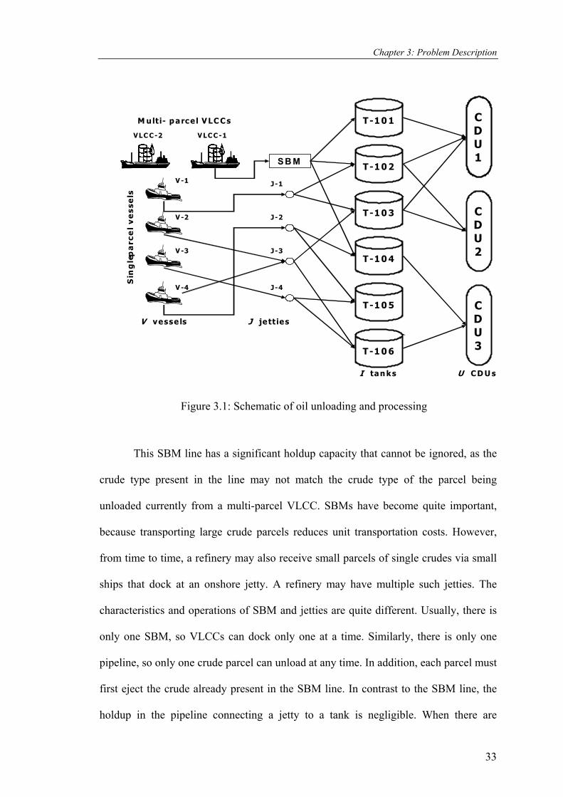
Chapter 3: Problem Description
SBM
T-10 1
T-10 2
T-10 4
T-10 3
T-10 5
T-1 0 6
CDU3
CDU2
CDU1
M ulti- p arcel V LC C s
VLC C-2 V LC C -1S
ing
le-p
arc
el
ve
sse
ls
V -1
V -2
V -3
V -4
J-1
J-2
J-3
J-4
V vesse ls J jetties
I tan ks U C D U s
Figure 3.1: Schematic of oil unloading and processing
This SBM line has a significant holdup capacity that cannot be ignored, as the
crude type present in the line may not match the crude type of the parcel being
unloaded currently from a multi-parcel VLCC. SBMs have become quite important,
because transporting large crude parcels reduces unit transportation costs. However,
from time to time, a refinery may also receive small parcels of single crudes via small
ships that dock at an onshore jetty. A refinery may have multiple such jetties. The
characteristics and operations of SBM and jetties are quite different. Usually, there is
only one SBM, so VLCCs can dock only one at a time. Similarly, there is only one
pipeline, so only one crude parcel can unload at any time. In addition, each parcel must
first eject the crude already present in the SBM line. In contrast to the SBM line, the
holdup in the pipeline connecting a jetty to a tank is negligible. When there are
33
Chapter 3: Problem Description
multiple jetties, multiple ships can dock at the same time and transfer crude parcels
simultaneously. In practice, pipelines also transport crude from marine terminals to
distant inland refineries or various petroleum products from refineries to far away
destinations (Rejowski and Pinto, 2003).
Many types of crude exist in the market, varying widely in properties,
processability and product yields. Years of experience have helped the refiners classify
crudes based on some key characteristics such as processability, yields of some
premium products, impurities or concentrations of some key components that influence
the downstream processing. This has led to the common practice of segregating crudes
(Kelly and Forbes, 1998) in both storage and processing. Thus, tanks and CDUs
usually store or process only specific classes of crudes. With this brief introduction, we
now state the crude scheduling problem.
3.2.1 Problem Statement
Given:
1) Arrival times of ships/VLCCs, volumes and crude types of their parcels
2) Configuration details (numbers of CDUs, storage tanks, jetties and their
interconnections) of the refinery
3) Holdup in the SBM pipeline and initial crude type
4) Limits on flow rates from the SBM station and jetties to tanks and from tanks to
CDUs
5) Limits on CDU processing rates
6) Storage tank capacities, their initial inventory levels and initial volume fractions of
crudes in tanks
7) Information about modes of crude segregation in storage and processing
34

Chapter 3: Problem Description
8) Information about key component concentration limits during storage and
processing
9) Economic data such as sea waiting costs, pumping costs, crude changeover costs,
etc.
10) Production demands during the scheduling horizon. These are normally available
from the monthly production plan of the refinery.
Determine:
1) A detailed unloading schedule for each VLCC / vessel
2) Inventory and composition profiles of storage tanks
3) Detailed crude charge profiles for CDUs
3.2.2 Operating Rules
Most refiners use some operating rules. In this work, we assume the following:
A tank receiving crude from another tank, a ship, or a tanker cannot feed a CDU at the
same time.
1) Each tank needs some time (8 h) for brine settling and removal after receiving
crude.
2) Multiple tanks can feed a single CDU. Most refiners allow at most two tanks to
feed a CDU, the operating complexity increases and operation controllability
becomes a problem for more than two in absence of individual tank flow control.
3) A tank may feed multiple CDUs. Again, a tank normally does not feed more than
two CDUs.
3.2.3 Assumptions
Finally, we make the following assumptions regarding the refinery operation:
1) Only one VLCC can unload at any moment. This is reasonable, as there is only one
SBM.
35

Chapter 3: Problem Description
2) The sequence in which a VLCC unloads its parcels is known a priori. A VLCC
always unloads parcels in the same sequence that it loads. Refinery planning,
which usually takes place weeks before the ship starts sailing towards the refinery
and the scheduling activity, predefines the loading sequence of parcels. Thus, the
parcel unloading sequence is indeed beyond the purview of crude oil scheduling
and this assumption is reasonable.
3) A parcel can unload to only one storage tank at any moment.
4) The SBM pipeline holds only one type of crude at any time and crude flow is plug
flow. This is valid, as parcel volumes in a VLCC are much larger than the SBM
pipeline holdup.
5) Crude mixing is perfect in each tank and time to changeover tanks between
processing units is negligible.
6) For simplicity, only one key component decides the quality of a crude feed to
CDU.
In the following section, we use several motivating examples to highlight the
drawbacks of existing approaches and the need for further work.
3.3 Motivating Examples
Three examples are considered to (1) provide some insight into the scheduling problem
(2) illustrate its complexity and (3) highlight the issues that previous work has failed to
resolve.
A refinery configuration (Figure 3.2) with four storage tanks (T1, T2, T3, and T4), two
CDUs (CDU1, CDU2) and one SBM line was considered. The refinery handles four
crudes (C1, C2, C3 and C4) and segregates them into two classes (Class1, Class2). As
shown in Figure 3.2, C1 and C2 belong to Class1; C3 and C4 belong to Class2; T1, T4
and CDU1 handle Class1 crudes; and T2, T3 and CDU2 handle Class2 crudes.
36
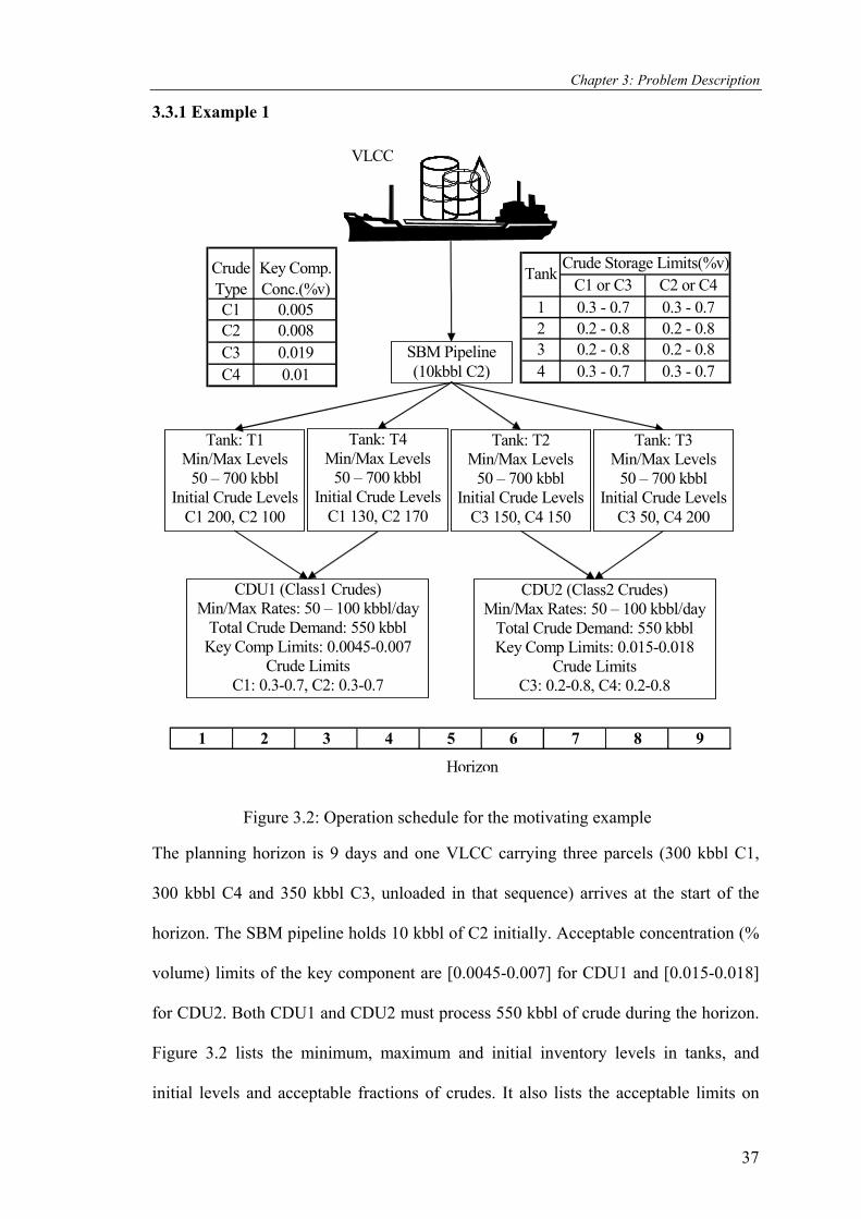
Chapter 3: Problem Description
3.3.1 Example 1
SBM Pipeline (10kbbl C2)
VLCC
Tank: T1 Min/Max Levels
50 – 700 kbbl Initial Crude Levels
C1 200, C2 100
CDU1 (Class1 Crudes) Min/Max Rates: 50 – 100 kbbl/day
Total Crude Demand: 550 kbbl Key Comp Limits: 0.0045-0.007
Crude Limits C1: 0.3-0.7, C2: 0.3-0.7
1 2 3 4 5 6 7 8 9
Horizon
Tank: T4 Min/Max Levels
50 – 700 kbbl Initial Crude Levels
C1 130, C2 170
Tank: T2 Min/Max Levels
50 – 700 kbbl Initial Crude Levels
C3 150, C4 150
Tank: T3 Min/Max Levels
50 – 700 kbbl Initial Crude Levels
C3 50, C4 200
CDU2 (Class2 Crudes) Min/Max Rates: 50 – 100 kbbl/day
Total Crude Demand: 550 kbbl Key Comp Limits: 0.015-0.018
Crude Limits C3: 0.2-0.8, C4: 0.2-0.8
C1 or C3 C2 or C41 0.3 - 0.7 0.3 - 0.72 0.2 - 0.8 0.2 - 0.83 0.2 - 0.8 0.2 - 0.84 0.3 - 0.7 0.3 - 0.7
Crude Storage Limits(%v)Tank
C1 0.005C2 0.008C3 0.019C4 0.01
Crude Type
Key Comp. Conc.(%v)
Figure 3.2: Operation schedule for the motivating example
The planning horizon is 9 days and one VLCC carrying three parcels (300 kbbl C1,
300 kbbl C4 and 350 kbbl C3, unloaded in that sequence) arrives at the start of the
horizon. The SBM pipeline holds 10 kbbl of C2 initially. Acceptable concentration (%
volume) limits of the key component are [0.0045-0.007] for CDU1 and [0.015-0.018]
for CDU2. Both CDU1 and CDU2 must process 550 kbbl of crude during the horizon.
Figure 3.2 lists the minimum, maximum and initial inventory levels in tanks, and
initial levels and acceptable fractions of crudes. It also lists the acceptable limits on
37

Chapter 3: Problem Description
crude fractions in the feeds to CDUs. The schedule is in periods of 1 day and the
objective is to maximize the gross profit, which is the difference between the marginal
profits of crudes and the operating cost. The operating cost includes sea-waiting cost
(or demurrage) of VLCC, crude-mix changeover losses and safety stock penalty. Sea
waiting cost is $10K per period (1 day), changeover cost is $5K per occurrence and
penalty is $0.2K per kbbl per period for depleting the total inventory beyond the
minimum stock of 1200 kbbl. The crude margins are $3K, $4.5K, $2K, and $4K per
kbbl of C1, C2, C3 and C4 respectively. We define crude margin as the total value of
crude cuts from a crude oil (not the final refinery products) minus the cost for
purchasing, transporting and processing the crude.
In many refineries, crude scheduling is a largely manual task with little
optimization. It is clear that a manual scheduling approach cannot effectively handle a
complex scheduling objective such as the one mentioned above. It is almost impossible
for the human scheduler to identify “optimal” crude mixes to process in each CDU.
Therefore, such an approach would normally aim to unload the parcels as early as
possible and then attempt to maintain constant feed rates to the CDUs, while
minimizing crude-mix changeovers. Table 3.1 shows a candidate schedule obtained
from such a strategy and the optimal schedule. Table 3.2 compares the profits of the
two schedules. In spite of having an extra changeover, the optimal schedule reduces
safety stock penalty, but more importantly, increases the profit by using crude mixes in
CDU2, which are more profitable. Even for this small example, rigorous optimization
increases the gross profit by 3.1%. In the face of narrow margins and intense
competition, this can make or break a refinery’s bottom line. Besides the above
example, previous work (Lee et al., 1996; Li et al., 2002, Kelley and Mann, 2002) has
also clearly established the benefits of optimized crude scheduling.
38
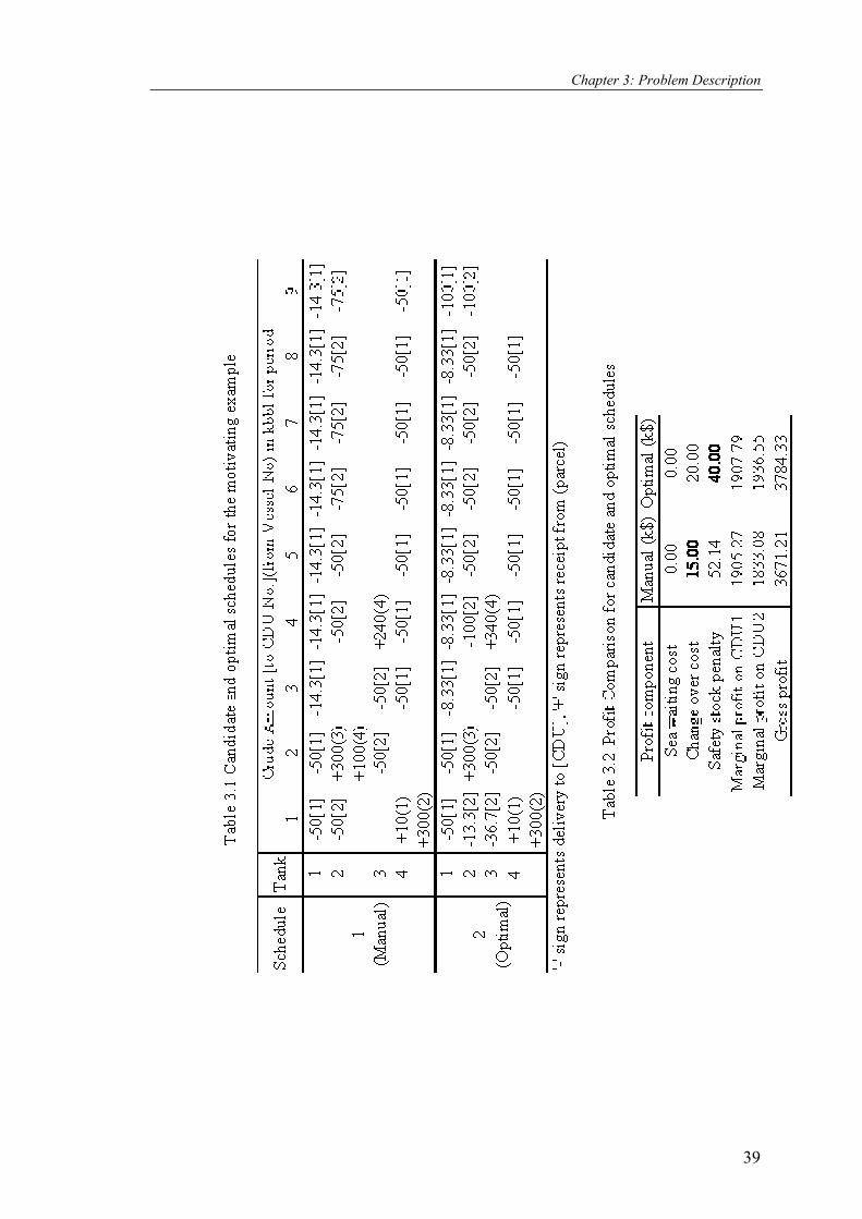
Chapter 3: Problem Description
39
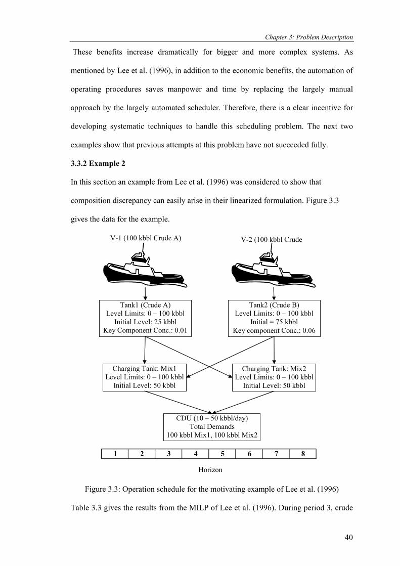
Chapter 3: Problem Description
These benefits increase dramatically for bigger and more complex systems. As
mentioned by Lee et al. (1996), in addition to the economic benefits, the automation of
operating procedures saves manpower and time by replacing the largely manual
approach by the largely automated scheduler. Therefore, there is a clear incentive for
developing systematic techniques to handle this scheduling problem. The next two
examples show that previous attempts at this problem have not succeeded fully.
Tank1 (Crude A) Level Limits: 0 – 100 kbbl
Initial Level: 25 kbbl Key Component Conc.: 0.01
Tank2 (Crude B) Level Limits: 0 – 100 kbbl
Initial = 75 kbbl Key component Conc.: 0.06
Charging Tank: Mix1 Level Limits: 0 – 100 kbbl
Initial Level: 50 kbbl
V-1 (100 kbbl Crude A)
CDU (10 – 50 kbbl/day) Total Demands
100 kbbl Mix1, 100 kbbl Mix2
1 2 3 4 5 6 7 8
Horizon
V-2 (100 kbbl Crude
Charging Tank: Mix2 Level Limits: 0 – 100 kbbl
Initial Level: 50
3.3.2 Example 2
In this section an example from Lee et al. (1996) was considered to show that
composition discrepancy can easily arise in their linearized formulation. Figure 3.3
gives the data for the example.
kbbl
Figure 3.3: Operation schedule for the motivating example of Lee et al. (1996)
Table 3.3 gives the results from the MILP of Lee et al. (1996). During period 3, crude
40

Chapter 3: Problem Description
in Mix1 has a key component concentration of 0.032. However, it is clear from Table
3.3; the feed from Mix1 to the CDU has a key component concentration of 0.024 in
period 3. The same happens during periods 5 to 8 in case of Mix2. One can also see
that a discrepancy also exists in the amounts of individual crude feeds to the CDU. For
instance, Table 3.3 shows that the CDU should receive 28 kbbl of crude A and 22 kbbl
of crude B in both periods 2 and 3. Instead, it receives 20 kbbl of A and 30 kbbl of B in
period 2 and 36 kbbl of A and 14 kbbl of B in period 3. Thus, in the MILP of Lee et al.
(1996), the crude composition in a feed tank may not match that in its feed to the CDU.
Furthermore, it is clear from Table 3.3 that the key component and crude
concentrations in the feed vary from period to period, even when they should remain
unchanged. For instance, the key component concentrations are 0.051, 0.052, 0.055
and 0.060 for periods 4 to 7 respectively for Mix2 feed. Similarly, as discussed above,
the delivered crude amounts are different in periods 2 and 3 for Mix1 feed. In short,
the MILP formulation of Lee et al. (1996) may lead to above two forms of
concentration discrepancy. The reason for the discrepancies in Lee et al. solutions is
evident. As discussed later in chapter 4, amounts of individual crudes that a charging
tank feeds must be in proportion to its composition. When the tank composition is
unknown, the constraints that enforce this requirement become bilinear. A discrete-
time formulation (e.g., that of Lee et al., 1996) that approximates these bilinear
constraints by linear ones will manifest the two discrepancies described above. This is,
because when the individual crude amounts (fed to CDU and held in tank) appear in
linear constraints only, the optimizer is free to feed individual crudes without regard to
their amounts in the tank. And, if there are no constraints that ensure that the tank
composition remains constant, when the tank receives no crudes, then the crude
amounts vary arbitrarily over periods also, as they are free to do so.
41
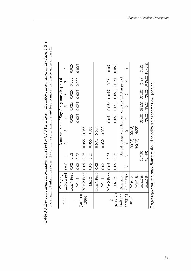
Chapter 3: Problem Description
42

Chapter 3: Problem Description
3.3.3 Example 3
Li et al. (2002) noted the first discrepancy as stated in the previous example and
proposed an iterative MILP/NLP approach to correct it. In their algorithm, they first
solve a MILP similar to Lee et al. (1996), whose solution may have the concentration
discrepancies. Based on that solution, they fix the vessel-to-tank and tank-to-CDU
allocation variables and replace the linearized crude blending constraints by the exact
nonlinear ones. This results in a NLP model, which they solve to correct the
compositions. Then, they use these compositions in the MILP and resolve the MILP
with correct linear composition constraints. Thus, they alternately solve MILP and
NLP, until they satisfy some termination criteria. The same approach was used to solve
the first motivating example (Figure 3.2) discussed earlier. Table 3.4 shows the crude
amounts fed to the two CDUs during various periods, as obtained by solving the first
MILP. It is clear that the delivered amounts vary from period to period and do not
respect the crude compositions in the tanks. Now, to correct this discrepancy, one must
solve a NLP by fixing the allocations given by the first MILP and using the correct
composition constraints. This means that the assignments of tanks for receipt and
delivery are fixed for each period. Surprisingly, it was found that the resulting NLP
was infeasible. A closer look revealed that T4 feeds CDU1 exclusively in periods 6-9.
Its composition is 29.5% C2 and 70.5% C1, which does not meet the quality
requirement (min 30% C2) for CDU1. To satisfy this quality requirement, both T1 and
T4 must feed CDU1 in some proportion. However, the NLP of Li et al. (2002) has no
freedom to change the tank-to-CDU allocations and hence cannot find a feasible
solution. This clearly demonstrates that Li et al.’s algorithm may not find a solution in
all cases, and reinforces the assertion of Kelly and Mann (2002) that a decomposition
strategy may fail to give a feasible solution, even though one exists.
43

Chapter 3: Problem Description
44

Chapter 3: Problem Description
45
Furthermore, a global optimal solution to NLP cannot be guaranteed in Li et al.(2002)
algorithm in all cases.
3.4 Outline
The discussion in the above sections points to the need for an improved methodology
for solving the crude scheduling problem. In the subsequent chapter, an MILP
formulation is developed using a discrete time representation to obtain an optimal
schedule for the abovementioned problem. At first, a complete MILP formulation is
developed for scheduling a refinery with one SBM line, I storage tanks and U crude
distillation units (CDUs). Then, the subsequent sections discuss the modifications
required to handle J jetties instead of one SBM line. The two formulations are merged
to obtain a formulation that accommodates one SBM line and J jetties. Then, the
formulation was modified to extend the model to allow a common practice of tank-to-
tank transfers.
Lastly, we present the novel solution algorithm, compare and contrast our model with
previous models and demonstrate application of our approach using a range of diverse
examples.

Chapter 4
MODEL FORMULATION – Discrete Time (part I)
4.1 Time Representation
To begin with, as in any scheduling problem, the time domain must be appropriately
represented. In the chemical scheduling literature, researchers have used primarily two
types of time representations - continuous and discrete. Both have their own
advantages and disadvantages. Most past attempts at this problem have also used
discrete representation of time. Pinto et al. (2000) suggested that although continuous-
time models reduce the combinatorial complexity substantially, discrete-time models
are still attractive, as they easily handle resource constraints and provide tighter
formulations. In this work, a uniform discrete-time representation is used. Let NT
identical periods (t = 1..NT) make up the scheduling horizon. 8 h periods are the best
choice, because most refineries operate in 8 h shifts and operators generally prefer to
synchronize the starts of critical tasks with the starts of shifts. Shorter periods can give
greater accuracy, but would increase the computational burden excessively.
For the sake of simplicity and to improve readability, we first develop a MILP
formulation for scheduling a refinery with one SBM line, I storage tanks and U crude
distillation units (CDUs). Then, we discuss the modifications required to handle J
jetties instead of one SBM line. In the next section, we merge the two to obtain a
formulation that accommodates one SBM line and J jetties. Lastly, we extend the
model to allow a common practice of tank-to-tank transfers.
46

Chapter 4: Model Formulation-Discrete Time
4.2 Unloading Via SBM
4.2.1 Parcel Creation
As the first step in the formulation, all arriving multi-parcel VLCCs are converted into
individual single-crude parcels. Before a VLCC can unload its first parcel, it must first
eject the crude residing in the SBM pipeline. This ejected crude will normally not
match the crude in the first parcel, hence one must treat it as a distinct single-crude
parcel and it must transfer (to a tank) before the first parcel from the VLCC. By the
same logic, the last parcel of a VLCC cannot transfer fully, because a portion equal to
the SBM line capacity must remain in the SBM line and cannot transfer until the next
VLCC starts unloading. As explained above, one must treat that portion as a distinct
single-crude parcel; call it an SBM parcel. In other words, unloading of each VLCC
results in an extra single-crude SBM parcel from its last parcel. This obviously reduces
the size of the last parcel in the VLCC. This gives an ordered list (order of unloading)
of all single-crude parcels, those in the VLCCs and their resulting SBM parcels. The
first parcel in this list is an SBM parcel that originated from the last VLCC that visited
the refinery in the past scheduling horizon. All parcels of the first VLCC to visit the
refinery in the scheduling horizon follow next, in the order of their unloading. The last
VLCC parcel will have a reduced size, but the SBM parcel that it created will follow
next. This continues for all VLCCs. At the end of the current scheduling horizon, the
SBM pipeline will hold the SBM parcel originating from the last parcel of the last
VLCC to visit the refinery in the current scheduling horizon. The list of parcels for the
current scheduling exercise excludes this parcel. To illustrate this parcel creation step,
consider a simple example with two VLCCs as in Figure 4.1. VLCC-1 has three
parcels: 250 kbbl Oman, 300 kbbl Murban and 110 kbbl Ratawi, which are to unload
in that sequence. VLCC-2 also has three parcels: 250 kbbl Escravos, 250 kbbl
47

Chapter 4: Model Formulation-Discrete Time
Forcados, and 250 kbbl Arabmix, which are to unload in that sequence. At start, the
SBM line holds 10 kbbl Kuwait. This is different from Oman in the first parcel of
VLCC-1, so 10 kbbl Kuwait in the SBM line be treated as a distinct parcel that must
unload first. Thus, the first three parcels in the list become 10 kbbl Kuwait, 250 kbbl
Oman and 300 kbbl Murban. The Ratawi parcel of VLCC-1 will be fourth in the list,
but with a reduced size of 100 kbbl, because 10 kbbl of Ratawi will remain in the SBM
line, until VLCC-2 ejects it. Thus, the remaining parcels (the fourth and later) in the
list become 100 kbbl Ratawi, 10 kbbl Ratawi, 250 kbbl Escravos, 250 kbbl Forcados,
and 240 kbbl Arabmix. Note that the last parcel (Arabmix of VLCC-2) has a reduced
size. The SBM parcel emanating from the Arabmix parcel will be first in the parcel list
for the next scheduling horizon. Thus, the list has two extra SBM parcels to model the
operation of an SBM line with nonzero holdup effectively.
SBMKuwait (10 kbbl)
#1Oman (250 kbbl)
#2Murban (300 kbbl)
#3Ratawi (110 kbbl)
#1Escravos (250 kbbl)
#2Forcados (250 kbbl)
#3Arabmix (250 kbbl)
VLCC-1
VLCC-2
#1SBM
Kuwait (10 kbbl)
#2Oman (250 kbbl)
#3Murban (300 kbbl)
#4Ratawi (100 kbbl)
#5SBM
Ratawi (10 kbbl)
#6Escravos (250 kbbl)
#7Forcados (250 kbbl)
#8Arabmix (240 kbbl)
SBM*Arabmix (10 kbbl)
(*For the next Scheduling horizon)
Figure 4.1: Schematic representation of parcel creation
48

Chapter 4: Model Formulation-Discrete Time
At the end of the parcel creation step, let there be NP parcels (p = 1..NP) in the list,
which will unload exactly in the order in which they appear in the list. The assignment
of an arrival time ETAp to parcel p is as follows. ETAp for a VLCC parcel is the arrival
time of its VLCC, while that for an SBM parcel is the arrival time of the next VLCC.
Having defined the periods and parcels, now the position is set for developing the
constraints in MILP formulation. Let us begin with the parcel unloading operations.
4.2.2 Parcel-to-SBM Connections
The SBM operation demands that each parcel connect to the SBM line to unload and
then disconnect after unloading. To model this process of connection/disconnection,
we define three binary variables:
XPpt = otherwise period during unloadingfor lineSBM the toconnected is parcela if
01 tp
XFpt = otherwise period ofstart at the lineSBM the toconnectsfirst parcela if
01 tp
XLpt = otherwise period of end at the lineSBM thefrom sdisconnect parcela if
01 tp
Based on ETAp, we can identify the periods in which a parcel p can possibly be
connected to the SBM line. Thus, we define XPpt, XFpt and XLpt only for (p, t) ∈ PT =
{(p, t) | parcel p may be connected to the SBM line in t}. The following constraints
relate these variables:
)1()1( −− −+= tppttppt XLXFXPXP (p, t) ∈ PT (4.1a)
pt ptXP XL≥ (p, t) ∈ PT (4.1b)
Now, we assume that each parcel connects to and disconnects from the SBM line once
and only once, so
∑t
ptXF = = 1 (p, t) ∈ PT (4.2a,b) ∑t
ptXL
49
Chapter 4: Model Formulation-Discrete Time
Eqs. 4.1a,b and 4.2a,b together ensure that XFpt and XLpt will be binary automatically,
when the XPpt are so. Therefore, we treat XFpt and XLpt as continuous variables. Using
these variables, the time TFp at which p connects and the time TLp at which it
disconnects are:
∑ −=t
ptp XFtTF )1( (p, t) ∈ PT (4.3a)
∑=t
ptp tXLTL (p, t) ∈ PT (4.3b)
As we indicate later in detail, eqs. 4.1- 4.3 represent a novel approach for dealing with
parcel unloading, which uses much fewer binary variables than other approaches (Lee
et al., 1996; Li et al., 2002) in the literature and gives full flexibility.
Although two parcels cannot connect to the SBM line at a given instance, a
parcel can disconnect and the next parcel connects during a period t. This would help
utilize fully the time available in a period in a discrete-time formulation and embed
some continuous-time features in such a formulation. In principle, several small
parcels can connect and disconnect in this manner in a given period, but for simplicity,
we allow at most two parcels to connect in one period by using,
∑p
ptXP ≤ 2 (p, t) ∈ PT (4.4)
TF(p+1) ≥ TLp – 1 (4.5)
Eq. 4.5 ensures that two parcels can connect in one period, only if the first of them
disconnects in that period.
Lastly, a parcel can unload only after its arrival time, therefore,
TFp ≥ ETAp (4.6)
4.2.3 SBM-to-Tank Connections
As mentioned earlier, most refineries segregate crudes. To effect this crude
segregation, we define a set PI = {(p, i) | tank i may receive crude from parcel p}.
50

Chapter 4: Model Formulation-Discrete Time
Now, in order to receive crude from a parcel, a tank must also connect to the SBM
line. To model this process, we use:
XTit = {1 if tank is connected to the SBM line during period 0 otherwise
i t
t
Clearly, a tank i cannot receive crude from a parcel during a period, unless the parcel is
connected to the SBM line during that period. Therefore, we define a 0-1 continuous
variable Xpit = XPptXTit, which is one, only when both parcel p and tank i are connected
to the SBM line during t. We linearize this nonlinear relation by using:
Xpit ≥ XPpt + XTit – 1 (p, t) ∈ PT, (p, i) ∈ PI (4.7)
pti
pit XPX 2≤∑ (p, t) ∈ PT, (p, i) ∈ PI (4.8a)
itp
pit XTX 2≤∑ (p, t) ∈ PT, (p, i) ∈ PI (4.8b)
The above constraints also ensure that Xpit will be binary, when XPpt and XTit are so.
As we allowed (eq. 4.5) at most two parcels to connect to the SBM line in one period,
we do the same for tanks:
2≤∑i
itXT (4.9)
Eqs. 4.5 and 4.9 would admit at most four sequential tank-parcel connections in one
period. In order to restrict such connections to exactly two, we further impose,
∑∑ ≤p i
pitX 2 (p, t) ∈ PT, (p, i) ∈ PI (4.10)
4.2.4 Tank-to-CDU Connections
For supplying its crude for processing, a tank must connect to one or more CDUs. We
model this connection by the following binary variable:
Yiut = { 1 if tank feeds CDU during period0 otherwise
i u
51

Chapter 4: Model Formulation-Discrete Time
Operating policies may dictate that a tank may not charge more than some (say two)
CDUs simultaneously and vice versa. Thus,
∑ ≤u
iutY 2 (i, u) ∈ IU (4.11a)
∑ ≤i
iutY 2 (i, u) ∈ IU (4.11b)
where, IU = {(i, u) | tank i can feed CDU u}. Similarly, most often in practice, a tank
cannot feed a CDU, when it is connected to the SBM line or is settling brine after
receiving crude. Assuming a brine settling time of 8 h or one period, we use,
2XTit + Yiut + Yiu(t+1) ≤ 2 (i, u) ∈ IU (4.12)
4.2.5 Crude Delivery and Processing
Having modeled the parcel-to-SBM, SBM-to-tank and tank-to-CDU connections, we
are ready to transfer crude between tanks and parcels, and tanks and CDUs. We first
consider the transfers from parcels to tanks. To this end, we define FPTpit as the
amount of crude transferred from parcel p to tank i during period t. This transfer can
occur, only when both tank i and parcel p are connected to the SBM line, and its
amount must satisfy some lower and upper limits:
pitUpipitpit
Lpi XFPTFPTXFPT ≤≤ (p, t) ∈ PT, (p, i) ∈ PI (4.13)
While the lower limit in the above is the holdup of the SBM line, the upper limit is
fixed by the pumping rates of crudes to various tanks. In the event that multiple
sequential transfers occur in the same period, the total time required for all transfers
must not exceed the period length, therefore,
1≤∑∑p i
Upi
pit
FPTFPT
(p, t) ∈ PT, (p, i) ∈ PI (4.14)
Lastly, each parcel p must unload fully during the scheduling horizon, so if PSp
denotes the size of parcel p, then
52
Chapter 4: Model Formulation-Discrete Time
∑ti
pitFPT,
= PSp (p, t) ∈ PT, (p, i) ∈ PI (4.15)
As with tanks, most refineries segregate CDUs too. Therefore, to see if a tank can feed
a CDU, we define sets IU = {(i, u) | tank i can feed CDU u} and IC = {(i, c) | tank i
may have crude c sometime during the horizon}. For delivering crude to CDUs, we
define FCTUiuct as the amount of crude c delivered by tank i to CDU u during period t.
Then, the total amount FTUiut of crude that tank i feeds to CDU u during t is,
( , )iut iuct
i c
FTU FCTU∈
= ∑IC
(i, u) ∈ IU (4.16)
The above amount can be nonzero, only when tank i is connected to CDU u during t,
and it must satisfy some lower and upper limits:
YiutLiuFTU ≤ FTUiut ≤ Yiut
UiuFTU (i, u) ∈ IU (4.17)
Because multiple tanks may feed one CDU, the total feed FUut to CDU u during t is,
FUut = (4.18) ( , )
iuti u
FTU∈∑
IU
This must be within the processing limits of CDU u, so,
Lut ut utFU FU FU≤ ≤ U (4.19)
In practice, the plant operation may know that its CDUs cannot process crude mixtures
with some extreme fractions of crudes. To impose such limitations, we use,
Ucuut
iiuct
Lcuut xcFUFCTUxcFU ≤≤ ∑ (i, u) ∈ IU, (i, c) ∈ IC (4.20)
where, and are the allowable lower and upper limits on the fraction of crude c
in the feed to CDU u. Similarly, the concentration of some key component must also
be within certain allowable limits for a CDU. If xk
Lcuxc U
cuxc
kc is the fraction of key component k
in crude c, then we ensure these limits by using,
utUku
i ckciuctut
Lku FUxkxkFCTUFUxk ≤≤ ∑∑ (i, u) ∈ IU, (i,c) ∈ IC (4.21)
53

Chapter 4: Model Formulation-Discrete Time
In real operation, one would want to minimize the upsets caused by changeovers of
tanks (thus crudes) feeding to a CDU. To detect such changes, we define a 0-1
continuous variable YYiut = YiutYiu(t+1), which is one, if tank i is connected to CDU u
during both periods t and (t+1). We linearize YYiut as follows,
YYiut ≥ Yiut + Yiu(t+1) – 1 (i, u) ∈ IU (4.22a)
YYiut ≤ Yiu(t+1) (i, u) ∈ IU (4.22b)
YYiut ≤ Yiut (i, u) ∈ IU (4.22c)
Then, for detecting the presence of a changeover on a CDU, we use,
COut ≥ Yiut + Yiu(t+1) – 2YYiut (i, u) ∈ IU (4.23)
When multiple tanks feed a CDU, the composition of feed can change simply
due to a change in the feed rates from various tanks. This would upset the CDU
operation. However, if only a single tank is feeding a CDU, then a change in its feed
rate would not upset the CDU. Therefore, to prohibit a change in composition, when
two tanks are feeding a CDU, we force the feed flow rates of individual tanks to
remain constant by using the following:
)1(]2[ +≥+−∑ tiuiuti
iut FTUFTUYYM (i, u) ∈ IU (4.24a)
iuttiui
iut FTUFTUYYM ≥+− +∑ )1(]2[ (i, u) ∈ IU (4.24b)
4.2.6 Crude Inventory
First, to identify the crude in parcel p, we define a set PC = {(p, c) | parcel p carries
crude c}. Using VCTict to denote the amount of crude c in tank i at the end of period t,
we get the following from a crude balance on tank i,
( 1)( , ) ,( , ) ( , )
ict ic t pit iuctp c p t i u
VCT VCT FPT FCTU−∈ ∈ ∈
= + −∑ ∑PC PT IU
(i, c)∈IC (4.25)
With this, the total crude level in tank i at the end of period t is given by,
54
Chapter 4: Model Formulation-Discrete Time
( , )it ict
i c
V VC∈
= ∑IC
T (4.26)
This must satisfy some upper and lower limits as,
Uiit
Li VVV ≤≤ (4.27)
Because of processing and operational constraints, crude fractions in tanks may be kept
in some limits as follows,
itUicictit
Lic VxtVCTVxt ≤≤ (4.28)
Crude is normally stored in floating roof tanks to minimize evaporation losses. Such a
tank requires a minimum crude level (or heel) to avoid damage to the roof, when the
tank goes empty. Due to the presence of heel, crudes usually accumulate in the tank
over time. However, a crude type with negligible volume fraction does not affect the
overall quality significantly. Thus, to limit the number of crudes in a tank, it is
advisable to retain only the crudes with significant volume fractions and normalize
their initial fractions in the tank accordingly. Recall that the number of crudes in a tank
affects the problem size.
4.2.7 Production Requirements
We can specify them in several ways. One simple way is to specify a crude throughput
demand for each CDU in each period as follows:
FUut ≥ Dut (4.29)
This obviously requires detailed data that may be difficult to obtain readily. A better
way is to specify a throughput demand over the entire horizon for each CDU or groups
of CDUs:
ut
ut DFU =∑ or DFUu t
ut =∑∑ (4.30a,b)
55
Chapter 4: Model Formulation-Discrete Time
In order to integrate the refinery supply chain, we specify demands for the products
rather than the crudes. Thus, if PDj denotes the maximum demand for product j during
the scheduling horizon, then
ji u c t
jcuiuct PDyFCTU ≤∑∑∑∑ (4.31)
where, yjcu is the fractional yield of product j from crude c processed in CDU u.
4.2.8 Scheduling Objective
We use the maximization of total gross profit as the scheduling objective. We define
this as the total marginal profit (netback) from crudes minus the operating cost. The
former is simply the value of products minus the purchase cost of crude. As mentioned
earlier, one aim of short-term crude scheduling is to exploit the benefits of
opportunistic crude mixes. We consider gross profit instead of operating cost as the
objective, because the former includes the effect of crude compositions and the
marginal profits from individual crudes, while the latter does not.
Since the product yields vary with crudes and CDUs, we define CPcu as the
marginal profit ($ per unit volume) from crude c processed in CDU u. Note that the
marginal profit does not include any operational costs. We consider these separately in
the scheduling objective as follows. First, a change in the feed composition upsets the
steady operation of a CDU. This is called a changeover. A changeover lasts a few
hours and leads to off-spec products or slops during the transition. In other words,
every changeover incurs some cost to the refinery and is undesirable. We let COC
denote the cost per changeover. Second cost in crude scheduling is the demurrage or
sea-waiting cost. The logistics contract with each shipping vessel stipulates an
acceptable sea-waiting period. If the vessel harbors beyond this stipulated time, then
demurrage (or sea-waiting cost) incurs. We let SWCv ($ per unit time) denote the
demurrage or sea-waiting cost for VLCC v. Third, although unloading of crudes does
56

Chapter 4: Model Formulation-Discrete Time
incur costs, we exclude them from our scheduling objective. This is because the
amount of crude imported is fixed for the scheduling horizon. Similarly, unlike
previous work (Lee et al., 1996; Li et al., 2002), we also do not include the crude
inventory cost, because the refiner normally makes the purchasing decisions far in
advance and these decisions are beyond the purview of the scheduling activity. Once
the refiner purchases crude, it becomes an integral part of the system and incurs
inventory cost irrespective of the scheduling. However, one inventory-related decision
does fall under the purview of scheduling activity. That is the desire of most refiners to
maintain a minimum stock of crude to guard against uncertainty. Let SS denote the
desired safety stock of crude and SSP the penalty ($ per unit volume per period) for
under-running the crude safety stock. Based on the above discussion, we obtain the
total gross profit as,
Profit = ∑∑∑∑∑∑∑∑ −−−t
tu t
utv
vi u c t
cuiuct SCCOCOCDCCPFCTU (4.32)
DCv ≥ (p, v) ∈ PV (4.33) vvpp SWCETDETATL )( −−
SCt ≥ SSP(SS –∑ ) (4.34) iti
V
where, ETDv is the estimated time of departure of VLCC v as agreed in the logistics
contract, PV = {(p, v) | parcel p is the last parcel in VLCC v}, DCv is the demurrage
cost for VLCC v and SCt is the stock penalty for period t.
This completes our formulation (eqs. 4.1a to 4.34) for a refinery with one SBM
pipeline. However, refineries often use jetties with or without an SBM. We need only
slight modifications in the above formulation to allow crude unloading via jetties. To
this end, we now present a formulation for a refinery with J identical jetties, but no
SBM line.
57

Chapter 4: Model Formulation-Discrete Time
4.3 Unloading via Jetties
Unloading via a jetty is quite analogous to the same via an SBM line except for some
differences. We assume that only single-crude vessels berth at jetties, so we can treat a
vessel berthing at a jetty as simply a single-parcel VLCC. In contrast to the SBM line,
the holdup in a jetty-to-tank transfer line is small and its effect on the composition of
the receiving tank is negligible. Thus, we need not consider any new parcels (such as
SBM parcels considered earlier) arising from this holdup. The connection /
disconnection process of a vessel to a jetty is analogous to that of a parcel to the SBM
except that we have J identical berths instead of one SBM station.
Based on the above discussion, it is clear that we can use all the variables in the
SBM formulation with their usual meanings to handle jetties. Thus, in the ensuing
formulation, we discuss only those constraints that are absent or different from the
previous formulation.
Firstly, to allow J vessels to berth and unload simultaneously, we must drop
eqs. 4.5 and 4.9 and modify eqs. 4.4 and 4.10 as follows,
ptp
XP∑ ≤ J (p, t) ∈ PT (4.4a)
∑∑ ≤p i
pitX 2 J (p, t) ∈ PT, (p, i) ∈ PI (4.10a)
We continue to use eqs. 4.8a,b to ensure that a parcel can unload to at most two tanks
in the same period and a tank can receive from at most two parcels in the same period.
This is mainly for simplicity; if facilities permit, we can increase the number as suited.
For multiple sequential transfers occurring in the same period, we replace eq. 4.14 by,
pitU
i pi
FPTFPT∑ ≤ 1 (p, t) ∈ PT, (p, i) ∈ PI (4.14a)
58
Chapter 4: Model Formulation-Discrete Time
pitU
p pi
FPTFPT∑ ≤ 1 (p, t) ∈ PT, (p, i) ∈ PI (4.14b)
This completes the extension of our formulation to a refinery with J jetties and
no SBM. Table 4.1 lists its required constraints. Having derived the separate
formulations for SBM and jetties, we now combine them into one formulation for a
refinery with both one SBM and J jetties.
4.4 Unloading Via SBM and Jetties
In this case, both multi-parcel VLCCs and single-parcel vessels will arrive at different
times during the scheduling horizon. We treat all of them as vessels. In essence, we
have two sets of vessels. One set of vessels unloads via the SBM line, while the other
unloads via the jetties. After we create the SBM parcels for the VLCCs as explained in
section 4.2.1, we have three types of parcels; namely SBM parcels, VLCC parcels and
jetty parcels. For convenience, we include the SBM parcels as the first parcels in the
subsequent VLCCs. Thus, we now have only VLCC parcels and jetty parcels, and we
use the appropriate constraints developed exclusively for each set. Let SP denote the
set of VLCC parcels and JP denote the set of jetty parcels.
As discussed earlier, eqs. 4.1a,b, 4.2a,b, 4.3a,b, 4.6, 4.7, and 4.8a,b hold for
both parcel sets, eqs. 4.5 and 4.9 hold for SP only, and eqs. 4.4a and 4.10a hold for JP
only. All other constraints are common to both SP and JP, except those (eqs. 4.14, and
4.14a,b) governing multiple sequential transfers within a period. Instead of eqs. 4.14
and 4.14a,b, we use eq. 4.14a for both SP and JP and add the following constraint,
1pit pitU
p ppi pi
FPT FPTFPT FPT∈ ∈
+∑ ∑SP JP
U ≤ (4.14c)
This completes the formulation for a refinery with both one SBM and J jetties, and we
are now ready to address the practical feature of tank-to-tank transfers.
59
Chapter 4: Model Formulation-Discrete Time
4.5 Tank-to-Tank Transfers
In practice, one may need to transfer crude from one tank to another to facilitate a
quick crude receipt and avoid demurrage. To model these transfers, we use the
following binary variable:
Zii′t = {1 if a crude exchange occurs between tanks and during period0 otherwise
i i t′
i′ > i, (i, i′)∈II
where, II = {(i, i′) | crude transfer between tank i and i′ is allowed}. Note that we
defined Zii′t only for combinations of i and i′ and not permutations. Furthermore, Zii′t
defines only the existence of a transfer, not its direction. To identify the number of
times a tank i exchanges crude with another tank in a given period, we define,
ZTit = ,( , ) ,( , )
ii t i iti i i i i i i i
Z Z′′ ′ ′ ′> ∈ > ∈
+∑ ∑II II
′ (4.35)
Tank-to-tank transfers do complicate operations and refiners use them, only when no
other option is possible. Therefore, we allow at most one tank-to-tank transfer in a
period.
ZTit ≤ 1 (4.36a)
iti
ZT∑ ≤ 2 (4.36b)
Note that ZTit will automatically be binary, so we treat it as a continuous variable.
Similarly, we restrict the total number of tank-to-tank transfers in the scheduling
horizon to a small number m by using,
itt i
ZT∑∑ ≤ 2m (4.37)
As we did earlier (eq. 4.12) with a tank receiving crude, we assume that a tank
involved in a tank-to-tank transfer cannot feed a CDU. Therefore,
1it iutZT Y+ ≤ (i, u) ∈ IU (4.38)
60

Chapter 4: Model Formulation-Discrete Time
So far, we addressed only the existence of a transfer, but neither its direction
nor amount. To model the direction and amount, we define a continuous variable
FCTTii′ct as the amount of crude c transferred from tank i to tank i′. FCTTii′ct is positive,
when the transfer is from i to i′, and vice versa. Of the two tanks engaged in a tank-to-
tank transfer, one must deliver and the other must receive, therefore,
FCTTii′ct + FCTTi′ict = 0 (i, i′) ∈ II (4.39)
With this, the total amount of a tank-to-tank transfer from i to i′ in period t becomes,
FTTii′t = ii ctc
FCTT ′∑ (i, i′) ∈ II (4.40)
To obtain the absolute amount AFTTii′t (i′ > i) of a tank-to-tank crude transfer, we use,
AFTTii′t ≥ FTTii′t i′ > i, (i, i′) ∈ II (4.41a)
AFTTii′t ≥ FTTi′it i′ > i, (i, i′) ∈ II (4.41b)
Clearly, AFTTii′t must be zero, when Zii′t is zero, and it must also have an upper limit,
so,
[ (1 )Uii t ii ii ii t ii i itAFTT FTT Z Zδ δ ]′ ′ ′ ′ ′ ′≤ + − i′ > i, (i, i′) ∈ II (4.42)
where, δii′ = 1 for i′ > i and zero otherwise, and Ui iFTT ′ denotes the maximum amount
of tank-to-tank transfer possible between i and i′ in a period. Having constrained the
absolute transfer amount, we can now constrain the individual crude transfer amounts.
We do this as follows:
max[ , ] max[ , ]ii t ic i c ii ct ii t ic i cAFTT xt xt FCTT AFTT xt xt′ ′ ′ ′− ≤ ≤ ′
i′ > i, (i, i′) ∈ II (4.43)
The above transfers modify the individual crude balance (eq. 25) as,
( 1)( , ) ( , )( , ) ( , )
( , )
ict ic t pit iuct i ictp c i u i ip t i c
i i II
VCT VCT FPT FCTU FCTT ′−′∈ ∈ ≠′∈ ∈′ ∈
= + − +∑ ∑ ∑PC IUPT IC
(i, c) ∈ IC (4.25a)
61

Chapter 4: Model Formulation-Discrete Time
62
Chapter 4: Model Formulation-Discrete Time
Lastly, we allow a tank to receive crude from both a parcel and another tank in
the same period, as long as the two transfers take place sequentially in the period.
Therefore,
1pitii tU
i i pii pi
FPTAFTTFTT FPT
′
′≠ ′
+∑ ∑ U ≤ (i, i′) ∈ II (4.44)
In brief, to allow tank-to-tank transfers in our formulation, we replace eq. 4.25
by 4.25a in our SBM/jetty formulation and add eqs. (4.35) to (4.44). Table 4.1 lists the
required constraints for various formulations. Tank transfers increase the problem size
and complexity drastically due to the additional decisions, variables and constraints,
making the problem compute intensive. Since the main goal of tank-to-tank transfers is
to avoid demurrage, it may be desirable to allow them only in a few periods. For
instance, one may allow them only in the period before the arrival and in periods
during the berthing of a vessel. In such a case, we impose eq. 4.25a only for such
periods and eq. 4.25 for the remaining periods.
We observed that it was possible to get a better schedule without tank transfers
than with because no transfer cost was included in objective function. To avoid such
discrepancy, one can include a penalty or cost (TTC) in the objective function for each
tank transfer operation. With this, the objective function becomes,
Profit = iuct cu v ut t iti u c t v u t t i t
TTCFCTU CP DC COC CO SC ZT2
− − − −∑ ∑∑ ∑ ∑∑∑∑∑∑
(4.32a)
The crude scheduling problem, as discussed here, is an inherently nonlinear
problem due to the blending of crudes in tanks. Our proposed linear formulations,
although novel, more general, and improved, as compared to previous work (Lee et al.,
1996; Li et al., 2002), are still approximations of the correct nonlinear formulations,
63

Chapter 4: Model Formulation-Discrete Time
64
and thus suffer from the discrepancies outlined earlier in the motivating examples. This
is because the constraints involving FCTUiuct are all linear and the optimizer is free to
push arbitrary amounts of individual crudes rather than the correct mixture to CDU.
This results in a disproportionate delivery of crudes to CDUs. In the next chapter, we
develop a novel iterative strategy to correct the concentration discrepancies without
solving any nonlinear problem.
Chapter 5
SOLUTION ALGORITHM – Discrete Time
To avoid concentration discrepancy in crude charge to CDU, one must use the correct
nonlinear constraint FCTUiuct = fict FTUiut, where fict is the fraction of crude c in tank i
at the end of period t. As discussed earlier in chapter 3, Li et al. (2002) proposed a
MILP/NLP iterative approach to solve this problem, but their approach cannot
guarantee convergence in all cases. We now develop a novel iterative strategy that
simply solves a series of MILPs of reducing size and complexity to obtain a near
optimal solution with no discrepancy in composition.
5.1 Description
The main idea behind our algorithm is as follows. First, observe that every tank
has blocks of contiguous periods during which its composition does not change. For
such a block, if we knew that constant composition (fic), then the nonlinear equation
(FCTUiuct = fic FTUiut) becomes linear. Solving such an MILP would yield a solution
with no composition discrepancy. Thus, for each tank, we can divide all periods into
two distinct blocks. One for which we know the tank compositions, and the other for
which we do not. For the former, we can use the exact linear constraints (FCTUiuct = fic
FTUiut) and for the latter, we can use the linear approximations as proposed in our
formulation. Second, observe that a tank’s composition changes, only when it receives
crude from a parcel or another tank, otherwise not. During most periods, the tank will
receive nothing; hence its composition will be constant. However, we must know the
constant composition to make the nonlinear flow constraint linear. To this end, our
knowledge of the initial compositions of tanks comes in handy. Because we know the
initial composition in each tank, we can identify one initial block of periods for which
65
Chapter 5: Solution Algorithm
the composition is constant and known. The length of this block will vary from tank to
tank and it could be as short as just one period for some tanks. However, this at least
provides a start for our algorithm. As a first try, we can use the exact linear constraints
for these first blocks of periods and linear approximations for the remaining periods
and solve the MILP. This would give us a solution that has no composition
discrepancy at least for the first block of periods on each tank. It will also give us the
compositions in all tanks at the end of each period in each block. We now identify the
first common block of periods for which we know the compositions in all tanks. We
freeze the schedule until the end of that block, and repeat the entire procedure for
scheduling the remaining periods. In other words, we now solve another scheduling
problem with a reduced horizon. In this manner, we get progressively longer and
longer partial schedules, free of composition discrepancies, by solving a series of
MILPs, until we have the complete schedule. We now describe the algorithm in full
detail.
5.2 Stepwise Methodology
For the time being, we disallow tank-to-tank transfers in describing the
algorithm (Figure 5.1). At each iteration of our algorithm, we divide the NT periods
into two sets. Set 1 includes all periods with t ≤ t* for some t*, and set 2 the rest. The
schedule (or all variables Yiut, Xpit, FTUiut, FCTUiuct, etc. in the MILP) for periods in set
1 is (are) fixed based on previous iterations. However, the MILP variables for periods
in set 2 are free. From the schedule for set 1, we know the tank compositions at the end
of period t* or t = t*. Let fic denote the fraction of crude c in tank i at t = t*.
66

Chapter 5: Solution Algorithm
*it≤
*
*
it
ict
V
*i ≤ *
it
*it
Set t* = 0
Compute fic = VCT
Identify t (t*< t )such that fic is constant
Solve MILP with constraint FCTUiuct=fic*FTUiut for t
Set t* = Mini [ ]
Fix MILP variables (Xpit, Yiut, FPTpit, FTUiut, FCTUiuct etc)
t*= NT?
Final Solution
Figure 5.1: Flow chart for the solution algorithm
Then, our iterative algorithm proceeds as follows:
1. Set t* = 0.
2. From the fixed schedule for t ≤ t*, compute fic for each tank i as fic = ict*
it*VVCT using
the known information (VCTict* and Vit*).
3. For each tank i, identify the latest period > t*it
* such that its composition is fic for all
periods t* < t ≤ t . We do this as follows. Let p′ denote the last parcel that was
unloaded (to any tank) before t
*i
*. Let ∆PSp′ denote the amount of crude remaining
in parcel p′. If p′ has been unloaded fully before t*, then ∆PSp′ = 0. Now, let p″
67
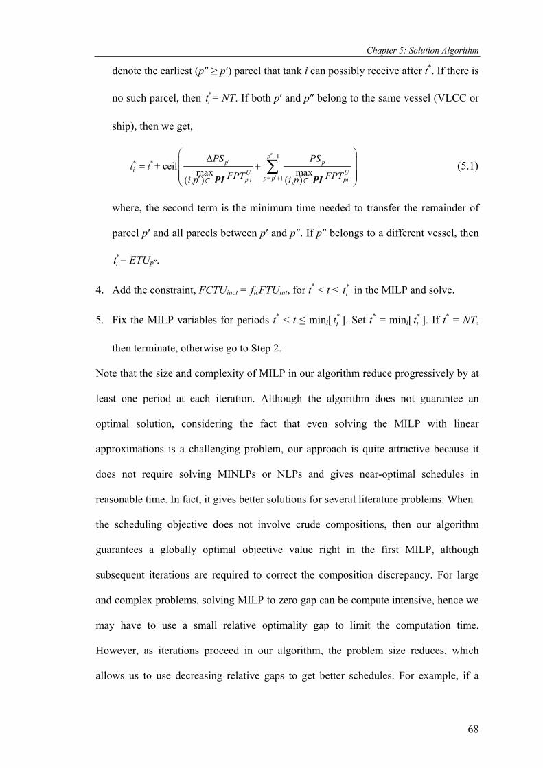
Chapter 5: Solution Algorithm
denote the earliest (p″ ≥ p′) parcel that tank i can possibly receive after t*. If there is
no such parcel, then t = NT. If both p′ and p″ belong to the same vessel (VLCC or
ship), then we get,
*i
∆x
)
1
1
+ ceil ma max( , ( , )
pp* *
i Up pp i pi
PS PSt t
FPT FPTi p i p
′′−′
′= +′
= + ′ ∈ ∈
∑PI PI
(5.1) pU
where, the second term is the minimum time needed to transfer the remainder of
parcel p′ and all parcels between p′ and p″. If p″ belongs to a different vessel, then
= ETU*it p″.
4. Add the constraint, FCTUiuct = ficFTUiut, for t* < t ≤ in the MILP and solve. *it
5. Fix the MILP variables for periods t* < t ≤ mini[ t ]. Set t*i
* = mini[ t ]. If t*i
* = NT,
then terminate, otherwise go to Step 2.
Note that the size and complexity of MILP in our algorithm reduce progressively by at
least one period at each iteration. Although the algorithm does not guarantee an
optimal solution, considering the fact that even solving the MILP with linear
approximations is a challenging problem, our approach is quite attractive because it
does not require solving MINLPs or NLPs and gives near-optimal schedules in
reasonable time. In fact, it gives better solutions for several literature problems. When
the scheduling objective does not involve crude compositions, then our algorithm
guarantees a globally optimal objective value right in the first MILP, although
subsequent iterations are required to correct the composition discrepancy. For large
and complex problems, solving MILP to zero gap can be compute intensive, hence we
may have to use a small relative optimality gap to limit the computation time.
However, as iterations proceed in our algorithm, the problem size reduces, which
allows us to use decreasing relative gaps to get better schedules. For example, if a
68

Chapter 5: Solution Algorithm
problem has NT = 30, then we can use a relative gap of 5% for the first few iterations
and 0% for the rest, as the MILP becomes easier to solve.
Tank-to-tank transfers are extremely difficult to handle, because they affect the
formulation size and algorithm efficiency immensely. Firstly, we need several
additional binary variables and constraints in the formulation to allow tank-to-tank
transfers. Because any crude in a given class can be in any tank, the crude transfer and
balance constraints must be written for all crudes of the given class. Furthermore, a
tank-to-tank transfer can occur in any period; therefore, a constant composition block
cannot be longer than one period. In other words, the algorithm must progress only one
period in each iteration, until the allowable number of transfers is exhausted. It is also
not wise to restrict the number of transfers, because it may be difficult to decide
whether to consume the available transfers early or save them for future. All these
make the problem extremely difficult.
We now demonstrate the efficacy of our solution algorithm using the
motivating example (chapter 3, example 1) and illustrate how our algorithm corrects
the discrepancy between the compositions of sent and delivered crudes.
5.3 Illustration
In the motivating example discussed earlier, the VLCC arrives at the start of the
scheduling horizon. The first parcel (p = 1) is the SBM parcel with crude C2 of class1.
The second is with crude C1 of class1, while the third and the fourth carry class2
crudes. Based on the parcel sizes and maximum possible transfer rates, we set the
earliest possible unloading periods for parcels as ETU1 = 1, ETU2 = 1, ETU3 = 2, and
ETU4 = = 2. For the first iteration, t* = 0, fic values are as in Table 5.1. Since no parcel
has begun unloading, p′ is undefined. Parcel 1 is the earliest parcel from which T1 and
T4 can receive crude, so p″ = 1 for both and = t = ETU*1t
*4 1 = 1. Similarly, parcel 3 is
69

Chapter 5: Solution Algorithm
Table 5.1: Details of individual iterations for the motivating example using the proposed algorithm
C1 or C3 C2 or C4T1 1 0.667 0.333T2 2 0.500 0.500T3 2 0.200 0.800T4 1 0.433 0.567T1 EOH 0.667 0.333T2 2 0.500 0.500T3 2 0.200 0.800T4 EOH 0.705 0.295T1 EOH 0.667 0.333T2 3 0.244 0.756T3 3 0.200 0.800T4 EOH 0.705 0.295T1 EOH 0.667 0.333T2 4 0.244 0.756T3 4 0.200 0.800T4 EOH 0.705 0.295T1 EOH 0.667 0.333T2 EOH 0.244 0.756T3 EOH 0.800 0.200T4 EOH 0.705 0.295
27 0.469
4 4 EOH 3784.33 20 0.469
3 3 4 3815.35
453879 1.235
2 2 3 3819.78 35 0.562
1 1 2
Composition f ic
0 0 1 3879 53 2.719
Mini[t i * ]MILP Profit (k$)
Number of Binary Variables
CPU Time
(s)
EOH: End of Horizon
Iteration t * Tank t i*
the earliest parcel from which T2 and T3 can receive crude, so t = = ETU*2
*3t 3 = 2.
Now, we impose FCTU1uc1 = f1cFTU1u1, FCTU4uc1 = f4cFTU4u1, FCTU2uc1 = f2cFTU2u1,
FCTU2uc2 = f2cFTU2u2, FCTU3uc1 = f3cFTU3u1, FCTU3uc2 = f3cFTU3u2 and solve the
MILP. MILP solution gives a profit of $3879K, which gives us an upper bound on the
globally maximum profit for the exact nonlinear problem.
In the second iteration, t*= mini[ t ] = 1, so we freeze the schedule for the first
period and compute f
*i
ic as in Table 6. At t* = 1, we find that both parcels 1 and 2 have
unloaded fully, therefore p′ = 2 for T1 and T4, ∆PSp′ = 0 and p″ does not exist. So we
get = = 9. For T2 and T3, p″ = 3 and using eq. 33, we get t = = 2. Then, we
compute f
*1t
*4t
*2
*3t
ic for all tanks at t* = 1 and impose the linear composition constraints for
70
Chapter 5: Solution Algorithm
period 2 for T2 and T3 and for periods 2-9 for T1 and T4. MILP solution gives a profit
of $3879K. Continuing the procedure, we get the detailed results in Table 5.1. Table
5.1 also shows the reduction in problem size with iterations. The algorithm terminates
after four iterations with a final profit of $3784.33K, which is within 2.44% of the
upper bound $3879K. This being a nonconvex MINLP problem, it is difficult to say
what the globally best solution is. Considering the fact that the best solution is surely
less than $3879K and we are achieving a solution within 2.44% of that without using
any NLP, we can safely consider our solution as near-optimal.
Before we illustrate our methodology on some real-life problems, a few
remarks highlighting the salient features of our formulation are in order.
5.4 Remarks
Our proposed formulations and solution approach differ significantly from previous
attempts at this problem.
1. The first major difference is that our formulation allows some features of a
continuous-time formulation in that tank-to-tank and parcel-to-tank transfers may
start at times other than period endpoints. This obviates partially the need for a
continuous-time formulation.
2. Unlike Li et al. (2002), our solution approach corrects composition discrepancy
without solving a single NLP, although the problem is inherently nonlinear. We
have already pointed out earlier that their decomposition strategy can fail to get a
solution. However, our algorithm fixes parcel-to-tank and tank-to-CDU allocations
based on corrected compositions, thus it cannot produce infeasible results.
3. Although we also model parcel-to-tank connections using bi-index binary
variables, our binary variables (XPpt and XTit) are subtly different from those (VTvt
and VIvi) of Li et al. (2002). The implications of this are quite subtle, but important.
71

Chapter 5: Solution Algorithm
While a vessel cannot deliver to multiple tanks during the scheduling horizon in Li
et al.(2002) formulation, this is possible in our formulation. To prove this point, let
us consider the allocation of vessel v to tank i at time t, as given by the variable
XWvit in Li et al. (2002). Li et al. (2002) defined VTvt and VIvi as:
VTvt = { 1 if vessel isconnected at time0 otherwise
v t
VIvi = { 1 if vessel isconnected to tank0 otherwise
v i
and fixed XWvit using the constraints: XWvit ≥ VTvt + VIvi – 1, XWvit ≤ VTvt and XWvit
≤ VIvi. Further, they allowed a vessel v to connect to only one tank i at any time t
by imposing viti
XW∑ ≤ 1. Now, consider a perfectly possible scenario in which a
vessel v delivers to tank T1 in period 1 and T2 in period 2. In this case, VTv1 = VTv2
= VIv1 = VIv2 = 1. The three constraints for fixing XWvit make XWv11 = XWv21 =
XWv12 = XWv22 = 1 and viti
XW∑ = 2 for the two periods in violation of the
constraint viti
XW∑ ≤ 1.
4. A similar comment also holds for tank-to-CDU allocation. Li et al. (2002) used bi-
index binary variables (ITit and ILil) to define CDilt by using CDilt ≥ ILil + ITit – 1,
CDilt ≤ ILil, CDilt ≤ ITit, and
ITit = { 1 if tank is connected at time0 otherwise
i t
ILil = { 1 if tank isconnected toCDU0 otherwise
i l
Suppose that tank T1 delivers to CDU1 in period 1 (CD111 = 1, CD121 = 0) and to
CDU2 (CD112 = 0, CD122 = 1) in period 2. Because T1 must connect to CDU1 and
CDU2 both, IL11 = IL12 =1. Similarly T1 must connect in both periods, so IT11 =
IT12 = 1. With these, the defining constraints for CDilt give CD121 = CD112 = 1,
72
Chapter 5: Solution Algorithm
73
which contradicts the assumed values. In other words, once a tank connects to a set
of CDU, it cannot connect to any other set of CDU during the scheduling horizon.
Even if we were to use bi-index binary variables of the form ITit and LTlt with time
dimension in both, it still would not allow all possible charging scenarios. Thus,
disaggregating tank-to-CDU binary variables limits the tank-to-CDU connections
and does not seem to offer any advantage. Our formulation, on the contrary, allows
all viable scenarios.
5. The existing literature (Lee et al., 1996; Li et al., 2002) defines changeover to arise
from a change in composition of feed to CDU. However, it ignores the fact that
composition may change, even when flows from two tanks feeding to one CDU
change. Our eqs. 4.22a-c and 4.23 describe the transitions accurately. When two
tanks deliver to one CDU, then change in flow from any tank also causes a
transition. To avoid such a transition, refiners keep the flows from both tanks
constant. Our eqs. 4.24a,b enforce this industry practice.
6. Unlike our formulation, the changeover constraints of Li et al. (2002) count two
changeovers, when a tank stops feeding a CDU and another starts feeding the
same. To illustrate this, consider that tank T1 stops feeding and T2 starts feeding to
CDU1 from period 3. Thus, the tank-to-CDU allocations are CD112 = CD213 = 1
and CD212 = CD113 = 0. Using Li et al. (2002)’s constraints, Zilt ≥ CDilt – CDil(t–1)
and Zilt ≥ CDil(t–1) – CDilt, we find that Z113 = Z213 = 1. In other words, even though
only one changeover occurs on CDU1, Li et al. (2002) count them as two, one for
each tank.
We now illustrate our methodology on several examples derived from a local refinery
configuration (SRC, Singapore). In order to maintain confidentiality, we used different
set of data but kept the nature of problem identical, employed similar operating rules.

Chapter 6
MODEL EVALUATION
6.1 Examples
We use Example-2 of Li et al. (2002) as our first example. For the remaining
examples, we take a refinery with 8 tanks (T1-T8), 3 CDUs (CDU1-CDU3) and two
classes (Class1 & Class2) of crudes. Tanks T1, T6, T7, T8 and CDU3 store/process
Class1 crudes, while the rest store/process Class2 crudes. We selected these examples
to illustrate the use of our models for refineries with different configurations (SBM,
jetties, tank-to-tank transfers), short and long scheduling horizons, and several parcel
sizes and arrivals. Example 1 compares the present approach to that of previous work
of Li et al. (2002) on this scheduling problem. Refinery configuration includes 7
storage tanks, four jetties and two CDUs. During 7 day horizon, refinery handles six
different types of crudes. The crude arrival data, economic data, and initial crude
inventory data for example 1 is given in Table 6.1, Table 6.2, and Table 6.3
respectively. Example 2 describes the refinery configuration with SBM and validates
the model. Example 3 uses the same configuration as of example 2 but with long
scheduling horizon. Example 4 illustrates the refinery configuration with multiple
jetties. Example 5 explains a refinery configuration with SBM and multiple jetties.
Lastly, example 6 demonstrates the feature of tank to tank transfers using a refinery
configuration with SBM and compares the schedule with that of no tank to tank
transfers. For examples 2 to 6, Table 6.4 gives the initial crude levels in tanks and their
capacities, Table 6.5 provides the initial crude compositions in tanks, Table 6.6
presents the tanker arrival details, crude demands and key component concentration
limits on CDUs, Table 6.7 furnishes the crude types, their marginal profits and key
74

Chapter 6: Model Evaluation
component details and Table 6.8 includes economic data and limits on crude transfer
amounts. Wherever possible, we compared our approach with the previous approaches
for these examples. We used CPLEX 7.0 solver within GAMS on a Gateway E5250
(Pentium II) machine running Windows NT. Table 6.9 gives the model statistics and
histories of model performance for all examples.
6.1.1 Data Tables
6.1.1.1 Example 1
Table 6.1: Crude arrival information for example 1
Vessel Capacity(MT)
Arrival time(Day) Crude type
1 3000 1 C12 3000 1 C13 3000 2 C14 3000 2 C15 5000 3 C16 5000 3 C17 3000 3 C18 3000 3 C19 3000 4 C1
10 5000 5 C211 5000 5 C212 3500 5 C213 3500 5 C214 3000 6 C115 3000 6 C116 3000 7 C417 1500 7 C217 1500 7 C6
Table 6.2: Crude types and processing margin for example 1
Crude Type
Crude cost (yuan)
Production cost (yuan)
C1 1130 2130C2 1574 2574C3 1418 2418C4 1150 2150C5 1150 2150C6 1671 2671
75

Chapter 6: Model Evaluation
Table 6.3: Initial crude inventory and storage capacities of storage tanks for example1
Tank T1 T2 T3 T4 T5 T9Min capacityMax capacity
Initial inventory 5000 5000 7000 8000 8000 10000 5000 5000 10000Crude Type C1 C2 C3 C1 C1 C2 C4 C6 C3
T6
40000250000 0
6.1.1.2 Examples 2-6
Ex2 to 4, 6 Ex 5 Ex2 to 4, 6 Ex 5 Ex2 to 4,[6] Ex 5T1 570 400 60 50 350 250T2 570 400 60 50 400 200T3 570 400 60 50 350 300T4 980 400 110 50 950 350T5 980 400 110 50 300 250T6 570 400 60 50 80[240] 100T7 570 400 60 50 80[120] 100T8 570 400 60 50 450[550] 250
Tank Capacity (kbbl) Heel (kbbl) Initial Inventory (kbbl)
Data in [] indicate the change in data for Ex6 from Ex2 to 4
Table 6.4: Initial crude levels, capacities of storage tanks for examples 2-6
C1or5 C2or6 C3or7 C4or8 C1or5 C2or6 C3or750 100 150 50 100 100 50
200 0 50 150 50 100 100100 100 50 100 100 100 100200 250 200 300 100 150 100100 100 50 50 100 75 75
20[30] 20[30] 20[150] 20[30] 25 25 5020[30] 20[30] 20[50] 20[10] 50 25 25
100[150] 100 100[210] 150[90] 75 75 100
Initial Crude Composition (kbbl)Example 2 - 4, [6] # Example 5 *
Data in [] indicate the change in data for Ex 6 from Ex 2 to 4 # Tanks 1, 6-8 store crudes 1-4; 2-5 store 5-8 for Ex 2-4 & 6 *Tanks 1, 6-8 store crudes 1-3 (Class 1); 2-5 store 4-6 (class 2) for Ex 5
Table 6.5: Initial crude composition in storage tanks for examples 2-6
76

Chapter 6: Model Evaluation
77

Chapter 6: Model Evaluation Chapter 6: Model Evaluation
78
6.1.2 Results and discussion
6.1.2.1 Example 1
For the sake of a fair comparison, we used the same definition of changeover,
objective function as used by Li et. al (2002) and a relative gap of 10% for MILPs. Our
approach yielded a different schedule (Table 6.10) with a 10.3% increase in profit
(Table 6.9), as compared to that reported by Li et al. (2002). Our approach solved
seven MILPs and took 94 s (Table 6.9), while their approach required four
(NLP+MILP)s and took 212 s with a profit of 97902225 Yuan. We also successfully
solved this example using a relative gap of 0.01% without much change in profit in
327 s of CPU time. Table 6.11 shows the berth allocation schedule in various periods.
Ex 61.5
1.71.51.6
1.451.6
1.551.6
bbl)
Table 6.7: Crude types, marginal profits and key component details for examples 2-6
Ex 2-4 Ex 5 Ex 6 Ex 2-4 Ex 5C1 0.002 0.005 0.0025 1.5 1.5
C2 0.0025 0.008 0.0025 1.7 1.75C3 0.0015 0.004 0.004 1.5 1.85C4 0.006 0.015 0.002 1.6 1.25C5 0.012 0.01 0.01 1.45 1.45C6 0.013 0.02 0.015 1.6 1.65C7 0.009 0.014 1.55C8 0.015 0.011 1.6
Crude Key comp. conc. (fr) Profit ($/
($/bbl/period)0.20.20.2
over Safe Inventory Penalty
ounts for examples 2-6
Parcel-Tk Tk-CDU Tk-Tk
(k$/period) (k$/instance)2 to 4 10 - 400 20-45(40~) 25 10
5 10 - 250 0 - 50 15 56 10 - 400 0 - 45 0 - 400 50 25
Ex
Flow Rate Limits (kbbl / Period)Demurrage
CostChange
LossMin - Max Min - Max Min - Max
Table 6.8: Economic data and limits on crude transfer am
~ Limit for example 3
78

Chapter 6: Model Evaluation
79

Chapter 6: Model Evaluation
80

Chapter 6: Model Evaluation
6.1.2.2 Example 2
This example involves one SBM line, 20 8-h periods and two VLCCs with three
parcels each. Table 6.12 shows the operation schedule. Some salient features of the
schedule are as follows:
1) T4 with a key component concentration of 0.0126 vol% cannot meet the feed
quality for CDU2, so the optimizer combined crudes from T4 and T5 (0.0123 vol
%) in periods 1, 2, 10, 11 and 12.
2) Two tanks feed a CDU in several periods. For instance, T6 and T7 feed CDU3 in
periods 5-10, T1 and T8 feed CDU3 in periods 11-14, and T4 and T5 feed CDU2
in periods 1, 2 10 and 12. At all times, the optimizer maintained the individual tank
feed flows constant to avoid a composition change. As mentioned earlier, many
refineries practice this.
3) Sequential, multiple transfers to one or more tanks occur in several periods. For
example, in period 1, parcels 1 (SBM) and 2 (1st parcel of VLCC-1) unload to T7.
In period 2, parcel 2 and parcel 3 (2nd parcel of VLCC-1) unload to T6. Lastly, in
period 3, parcel 3 and parcel 4 unload to T7 and T3 respectively. This is a
continuous-time feature in our formulation.
4) T4 delivers to both CDU1 and CDU2 in periods 1, 2, 10, 11 and 12.
5) T2 receives crude in period 14, uses period 15 for brine settling and removal, and
starts delivering in only period 16. T7 does the same in periods 4, 5 and 6.
6) Lastly, we see from Figure 6.1 that the key component concentration in feed
changes, only when a changeover occurs.
Table 6.13 details profit, CPU time and actual/target relative gaps for iterations.
81

Chapter 6: Model Evaluation
82

Chapter 6: Model Evaluation
) Target Actual
1 3427.60 146.5 5.0 4.62 3454.86 292.9 3.5 3.43 3495.37 836.3 3.5 2.04 3444.32 70 3.5 2.85 3433.12 7.8 2.0 1.66 3439.00 9.8 0.0 0.07 3424.90 0.74 0.0 0.0
MILPIteration
Profit (k$)
CPU Time (s)
Relative Gap (%
Table 6.13: Solution details for Example 2
1.255
1.260
1.265
1.270
0 5 10Time period
Key
Com
p (%
Vol
)
Key comp. inCDU1 feed
1.220
1.225
1.230
1.235
1.240
1.245
1.250
0 5 10 15Time Period
Key
Com
p.(%
Vol
)
Key Comp inCDU2 feed
0.310.315
0.320.325
0.33
0.3350.34
0.3450.35
0 5 10 15Time period
Key
Com
p. (%
Vol
)
Key comp. inCDU3 feed
Figure 6.1: Key component concentration in CDU feeds at various
time periods for example 2
15 20
20
20
83

Chapter 6: Model Evaluation
6.1.2.3 Example 3
To demonstrate our algorithm’s ability to solve larger problems, we consider a longer
horizon of 42 periods for Example 2, with three VLCCs carrying three parcels each.
Table 6.14 shows the operation schedule. The schedule shows all the salient features as
explained in the previous discussion for example 2. The model performance (Table
6.9) reveals that longer horizon problems are highly compute-intensive and consume
nger CPU time. These problems may require higher relative gaps for the first few
MILPs in order to get quicker solutions. Such problems can be solved easily using
increased period lengths which in turn reduce total number of decision variables,
allowing quicker solution but would approximate the decision making, leading to
practical difficulties in its actual realization. Continuous time modeling approach could
be helpful in solving longer horizon problems and needs to be explored.
6.1.2.4 Example 4
In this example, we consider three jetties, no SBM, 15 8-h periods and 8 single-parcel
vessels (V1 to V8). Table 6.15 shows the operations schedule, while Table 6.16 shows
the berth allocations for the arriving vessels. Among some salient features of this
schedule, we have two jetties letting two vessels (V3 & V4) unload simultaneously to
(T3 & T6) and then to (T5 & T6) in period 6. Also in period 6, V3 unloads to both T3
& T5. In period 11, two vessels (V7 & V8) unload simultaneously to two different
tanks (T7 and T2 respectively). From periods 5 to 13, T1 & T8 feed CDU3 and we can
see that the composition of feed remains same during this period. The optimizer
achieved this by keeping flows from individual tanks constant. Thus, in addition to
showing ltaneous
berth allocations of multiple ansfers to multiple tanks in a
eriod.
lo
all the features mentioned in Example 2, the schedule shows the simu
vessels and simultaneous tr
p
84

Chapter 6: Model Evaluation
85
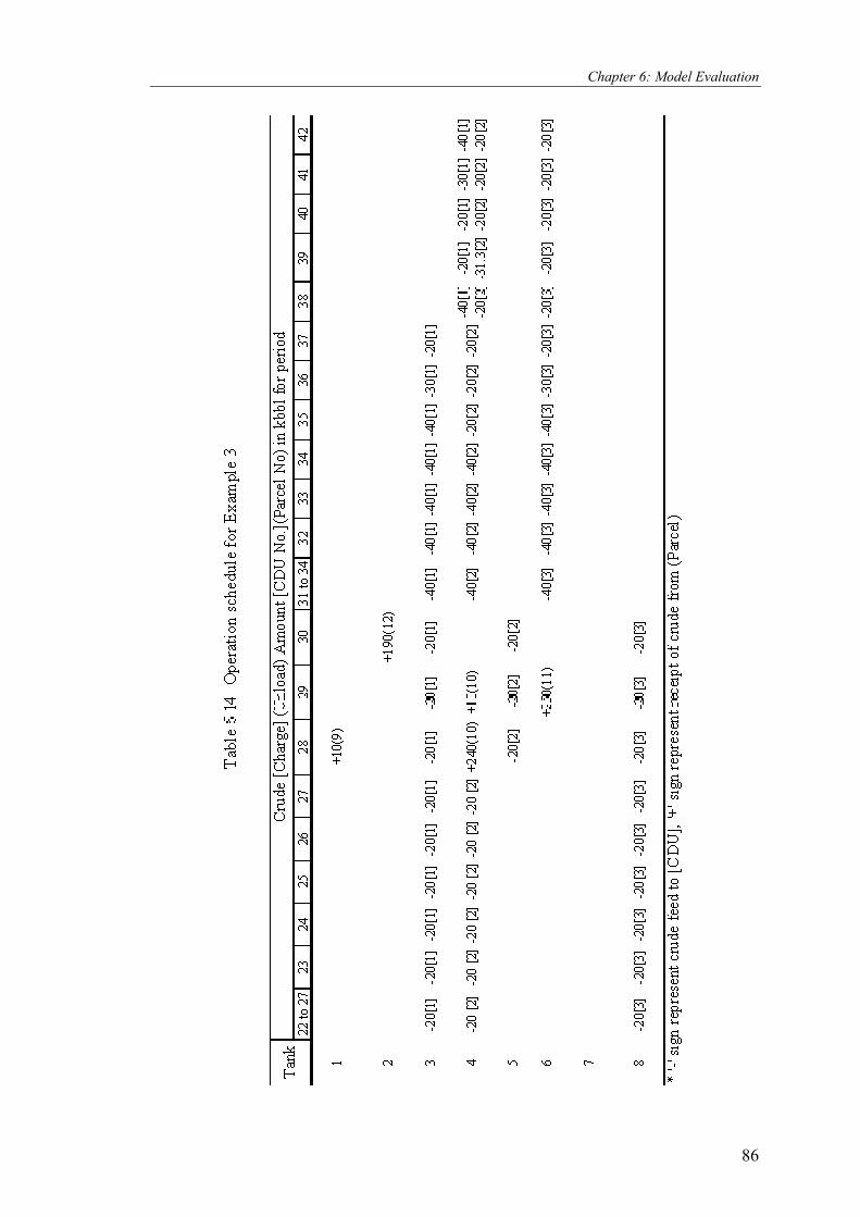
Chapter 6: Model Evaluation
86

Chapter 6: Model Evaluation
87

Chapter 6: Model Evaluation
6.1.2.5 Example 5
In this example, we consider two jetties, one SBM, 15 8-h periods, one VLCC with
three parcels and three single-parcel tankers. Table 6.17 shows the schedule. Since the
refinery has both SBM and multiple jetties, both should be able to transfer crude
simultaneously in any period. This example shows this feature in period 5, when parcel
4 from the VLCC and parcel 6 from V2 unload to T2 and T5. Similarly, during periods
6 & 7, parcels 5 & 7 from V1 and V3 simultaneously unload to T7 & T8. We have a
few instances of multiple tanks feeding one CDU: T2 and T4 feed CDU1 during
periods 11-15 and T2 and T5 feed CDU2 during the same time.
6.1.2.6 Example 6
In this example, we illustrate the benefits of tank transfer operations. We consider one
SBM, 10 8-h periods and one VLCC with three parcels. Table 6.18 gives the schedules
for the case with tank-to-tank transfers and for the case without them. For the former,
we allowed at most one tank transfer in periods 1-2 only. Note that the last parcel
unloads in period 6 for the latter, while the same unloads in period 5 for the former.
The optimal schedule for the former shows a transfer of 70 kbbl from T6 to T7 during
period 1. This transfer creates the required space and facilitates early unloading of
parcel. Thus, the last parcel unloads in period 5 and demurrage is avoided.
Furthermore, the profit with transfers is 2.7% greater than that without transfers.
Therefore, tank transfers provide additional flexibility to improve profitability. As
mentioned in chapter 4 section 4.5, tank-to-tank operations require more CPU resource
because it increases the problem size drastically due to additional decisions, variables
and constraints. Compared to previous examples, example 6 has less configurational
complexity but has more operational complexity and required more CPU resource.
88
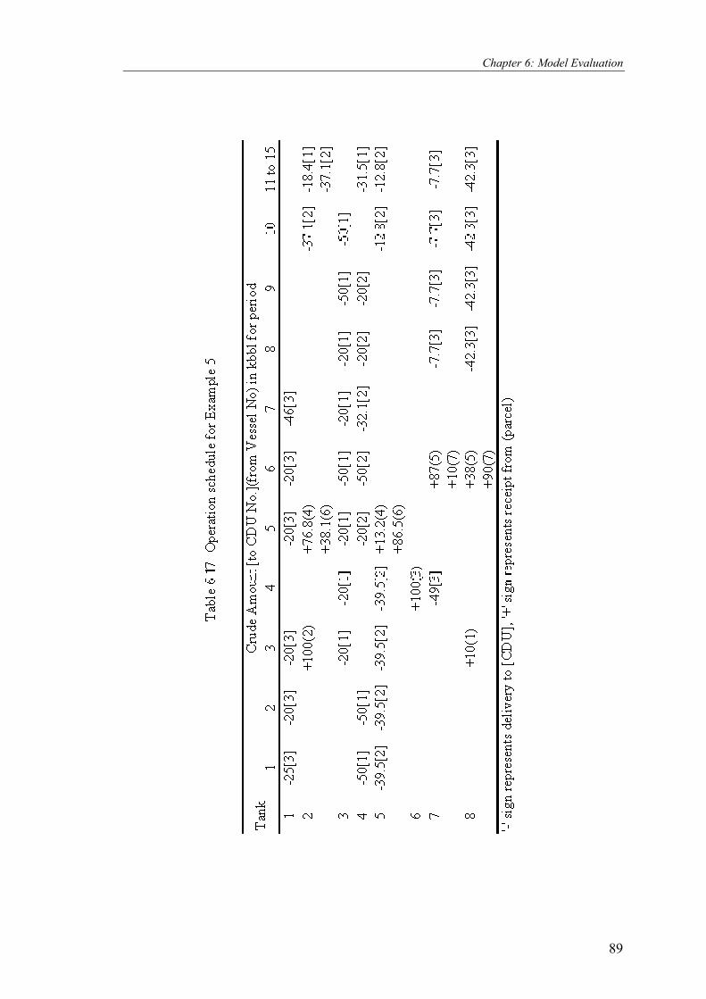
Chapter 6: Model Evaluation
89

Chapter 6: Model Evaluation
90
Chapter 6: Model Evaluation
6.2 Conclusion
Six examples are used to illustrate the use of our models for refineries with different
configurations (SBM, jetties, tank-to-tank transfers), short and long scheduling
horizons, and several parcel sizes and arrivals. The solution analysis of these examples
shows no discrepancy in composition. In addition to, they explain most of real life
operational features such as multiple tanks feeding one CDU, one tank feeding
multiple CDUs, SBM pipeline, brine settling, tank-to-tank transfers etc. This work uses
fewer binary variables and is different from and superior (both in terms of efficiency
and quality of solutions) to those reported in previous work. The proposed approach
helps quicker and near-optimal decision making in refinery operations and handles
problems with up to 14 days. The solution analysis of example 3, a longer horizon
problem, shows the limitation of this approach to yield early solutions. The tank to
tank feature (Example 6) is explained here, provides a real benefit but is highly
compute intensive. This reveals that the crude scheduling problem is a difficult,
nonlinear problem and it needs further work to be able to solve problems with longer
scheduling horizons in reasonable time.
91
Chapter 7
MODEL FORMULATION - Continuous Time (Part-II)
7.1 Introduction
In the previous chapters we developed a hybrid model and an iterative solution
algorithm for crude scheduling problem. The hybrid model is based on discrete time
approach with some continuous time features. We identified and addressed the
inherent problem of nonlinearity associated with crude blending operation and
efficiently handled them using the proposed an iterative, hybrid, discrete-time MILP
model. Additional real-world refining operational features such as single buoy
mooring (SBM) pipeline, jetties, and tank-to-tank transfers were also considered. The
number of binary allocation variables was reduced and 0-1 continuous variables
introduced to facilitate improved solutions to bigger problems. One attractive feature
of the model is that time continuity is approximated by allowing more than one
unloading allocation in any time period; thus the entire time period is utilized to the
maximum extent, when possible and the need for smaller time intervals is eliminated.
While the above approximation provides an attractive solution to handle time
continuity in a discrete formulation, another family of scheduling models uses an
inherent continuous-time representation so that the need for predefined, identical slots
is obviated. In these models, each activity’s start- and end-time are variables that the
model solution determines. So far, only discrete-time formulations have stood up to the
challenge of this important, nonlinear problem. A continuous-time formulation would
portend numerous advantages; however, existing work in this area has just begun to
scratch the surface. The continuous-time modeling is particularly suited to crude oil
92

Chapter 7: Model Formulation - Continuous Time
scheduling since refinery activities can range from a few minutes to several hours (Joly
et al., 2002). A discrete-time model would necessitate a large number of slots and
increase the computational complexity of the problem. Thus, the main advantages
(Pinto et al., 2000) of a continuous-time representation are the full utilization of time
continuity and the possibly reduced computational complexity due to fewer binary
variables.
Joly et al. (2002) proposed a continuous-time formulation for the refinery
scheduling problem, but their communication did not provide details of their model or
objective function. Jia and Ierapetritou (2003) also addressed the short-term scheduling
of refinery operations based on a continuous-time formulation. They divided refinery
operations into three sub problems, the first involving crude oil operations, the second
dealing with other refinery processes and intermediate tanks, and the third related to
finished products and blending operations. They addressed only the first subproblem in
which they used the component balance of Lee et al. (1996), which suffers from the
composition discrepancy mentioned earlier. They did not consider the changeover
costs arising from crude class or tank changes. Change of crudes and/or tanks is an
important operational activity in the refinery, which results in production losses and
slop creation. Their proposed model does not allow many operational features such as
multiple tanks feeding one crude distillation unit (CDU), single tank feeding multiple
CDUs, settling time for brine removal after crude receipt, etc. Besides, their demurrage
accounting may be inaccurate, as they seem to compute demurrage for the total time
that a vessel spends for unloading crude.
Magalhães and Shah (2003) also proposed a continuous-time model for crude
oil scheduling. While the details of algorithm and model were not reported, they
espoused real-world operational rules such as crude segregation, non-simultaneous
93
Chapter 7: Model Formulation - Continuous Time
receipt and delivery of crude by a tank, and settling time for brine removal. They
scheduled to achieve the target crude throughput over the scheduling horizon, but did
not consider crucial practical aspects such as demurrage and changeover. However,
they did acknowledge the importance of these aspects in making the problem realistic.
As the above discussion suggests, none of the reported continuous-time
formulations satisfactorily addresses the composition discrepancy in crude charge to
CDU, transfer lines with non-negligible volumes, and other important features such as
demurrage, changeovers, brine settling time, etc. This has given a motivation for
developing a continuous-time formulation that accommodates some of these
industrially important structural and operational features of a refinery.
In this research effort, we present the first complete continuous-time mixed
integer linear programming (MILP) formulation for the short-term scheduling of
operations in a refinery that receives crude from very large crude carriers via a high-
volume SBM (Single buoy mooring) pipeline. This novel formulation accounts for
real-world operational practices. We also employ a realistic profit-based objective
function that includes marginal crude profits, safety stock penalties, and accurate
demurrage accounting. We use an iterative algorithm similar to that developed for
discrete approach, to eliminate the crude composition discrepancy that has proven to
be the Achilles heel for existing formulations. While it does not guarantee global
optimality, the algorithm needs only MILP solutions and obtains excellent maximum-
profit schedules for industrial problems with up to seven days of scheduling horizon.
We also report the first comparison of discrete-time vs. continuous-time formulations
for this complex problem.
94

Chapter 7: Model Formulation - Continuous Time
7.2 Refinery configuration
In this work we considered a refinery configuration with SBM. Figure 7.1 gives
a schematic of the crude oil unloading, storing and processing in a typical refinery. The
SBM
T1
T2
T4
T3
T5
T6
CDU3
CDU2
CDU1
V Multi-Parcel VLCCs
I Tanks U CDUs
SBM
T1
T2
T4
T3
T5
T6
CDU3
CDU2
CDU1
V Multi-Parcel VLCCs
I Tanks U CDUs
Figure 7.1: Schematic of oil unloading using SBM and processing in CDUs
configuration involves crude offloading facilities such as an SBM (Single Buoy
Mooring) or SPM (Single Point Mooring) station, storage facilities such as storage
tanks and/or charging tanks and processing facilities such as crude distillation units
(CDUs). The operation involves unloading crudes into multiple storage tanks from the
ships/tankers arriving at various times and feeding the CDUs from these tanks at
various rates over time. Thus, the problem involves both scheduling as well as
allocation issues. The problem description is same as explained in chapter 2, here we
are attempting to find a solution using continuous time modeling approach.
7.3 MILP Formulation
7.3.1 Time Representation
Time representation is a key to continuous-time formulation. We employ a mix
of the strategies used by Karimi and McDonald (1997) and Lamba and Karimi (2002)
95

Chapter 7: Model Formulation - Continuous Time
in that we use synchronized (across tanks) but variable-length time slots within periods
defined by known, fixed time events. To this end, we first use the fixed time events to
divide the scheduling horizon into several periods with different lengths. In this paper,
we use two types of time events, but one could easily use more. These are the
scheduled arrival times of VLCCs and their latest expected departure times. We take
the latest expected departure time to be some hours later than the latest time by which
a VLCC must leave to avoid demurrage as stipulated in the VLCC’s logistics contract.
The first period begins at time zero and ends at the arrival time of the first VLCC. The
second period follows the first period and ends at the latest expected departure time of
the first VLCC. The next period ends at the arrival time of the second VLCC, and the
remaining periods follow likewise. The last period runs from the latest expected
departure time of the last VLCC to the end of the scheduling horizon. We use Dt (t = 1
… NT, D0 = 0) to denote the start of period t.
Having defined the periods, we now divide each period into a fixed number of
variable-length slots that are synchronized or identical across all storage tanks. The
numbers of slots may vary from period to period, but they are the same for all tanks.
As in most slot formulations, we must guess the number of slots for each period.
During a given slot, there is no activity change in any tank, i.e. the refinery state
remains unchanged during the entire slot. However, an activity may continue over two
consecutive slots on a given tank.
We consider a refinery with i tanks and u CDUs and one SBM line. If NV
VLCCs arrive during the scheduling horizon, then we have at most 2NV+1 periods.
We assign St slots to period t to get NS = S1 + S2 + … + SNT slots in the entire
scheduling horizon. We now derive constraints that govern different aspects of the
refinery crude operations.
96
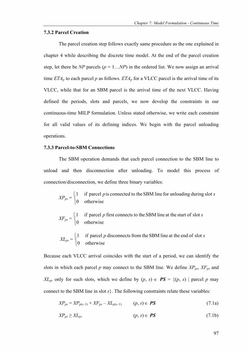
Chapter 7: Model Formulation - Continuous Time
7.3.2 Parcel Creation
The parcel creation step follows exactly same procedure as the one explained in
chapter 4 while describing the discrete time model. At the end of the parcel creation
step, let there be NP parcels (p = 1…NP) in the ordered list. We now assign an arrival
time ETAp to each parcel p as follows. ETAp for a VLCC parcel is the arrival time of its
VLCC, while that for an SBM parcel is the arrival time of the next VLCC. Having
defined the periods, slots and parcels, we now develop the constraints in our
continuous-time MILP formulation. Unless stated otherwise, we write each constraint
for all valid values of its defining indices. We begin with the parcel unloading
operations.
7.3.3 Parcel-to-SBM Connections
The SBM operation demands that each parcel connection to the SBM line to
unload and then disconnection after unloading. To model this process of
connection/disconnection, we define three binary variables:
XPps = otherwise
slot during unloadingfor line SBM the toconnected is parcel if01 sp
XFps = otherwise
slot ofstart at the line SBM the toconnectsfirst parcel if01 sp
XLps = otherwise
slot of end at the line SBM thefrom sdisconnect parcel if01 sp
Because each VLCC arrival coincides with the start of a period, we can identify the
slots in which each parcel p may connect to the SBM line. We define XPps, XFps and
XLps only for such slots, which we define by (p, s) ∈ PS = {(p, s) | parcel p may
connect to the SBM line in slot s}. The following constraints relate these variables:
XPps = XPp(s–1) + XFps – XLp(s–1) (p, s) ∈ PS (7.1a)
XPps ≥ XLps (p, s) ∈ PS (7.1b)
97
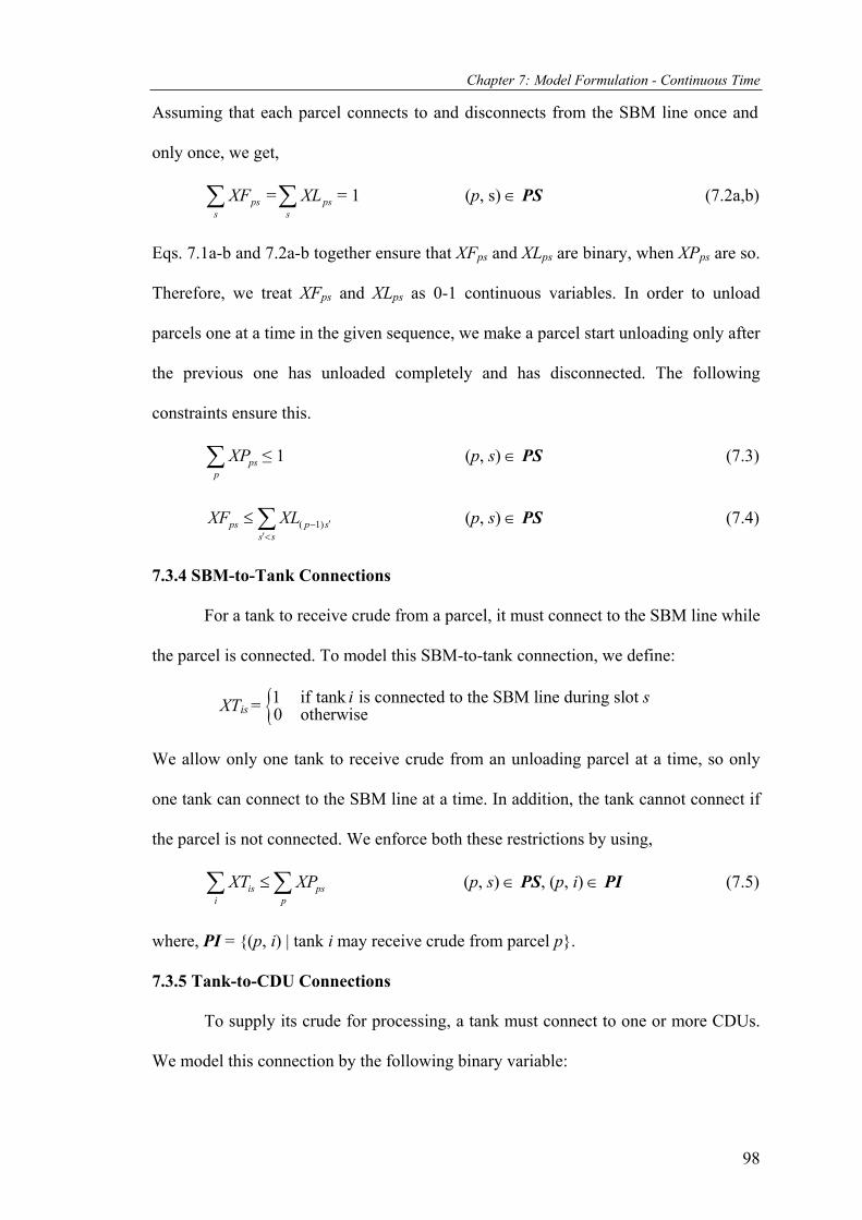
Chapter 7: Model Formulation - Continuous Time
Assuming that each parcel connects to and disconnects from the SBM line once and
only once, we get,
∑s
psXF = = 1 (p, s) ∈ PS (7.2a,b) ∑s
psXL
Eqs. 7.1a-b and 7.2a-b together ensure that XFps and XLps are binary, when XPps are so.
Therefore, we treat XFps and XLps as 0-1 continuous variables. In order to unload
parcels one at a time in the given sequence, we make a parcel start unloading only after
the previous one has unloaded completely and has disconnected. The following
constraints ensure this.
psp
XP∑ ≤ 1 (p, s) ∈ PS (7.3)
( 1)ps p ss s
XF XL ′−′<
≤ ∑ (p, s) ∈ PS (7.4)
7.3.4 SBM-to-Tank Connections
For a tank to receive crude from a parcel, it must connect to the SBM line while
the parcel is connected. To model this SBM-to-tank connection, we define:
XTis = {1 if tank is connected to the SBM line during slot 0 otherwise
i s
We allow only one tank to receive crude from an unloading parcel at a time, so only
one tank can connect to the SBM line at a time. In addition, the tank cannot connect if
the parcel is not connected. We enforce both these restrictions by using,
is psi p
XT X≤∑ ∑ P (p, s) ∈ PS, (p, i) ∈ PI (7.5)
where, PI = {(p, i) | tank i may receive crude from parcel p}.
7.3.5 Tank-to-CDU Connections
To supply its crude for processing, a tank must connect to one or more CDUs.
We model this connection by the following binary variable:
98

Chapter 7: Model Formulation - Continuous Time
Yius = { 1 if tank feeds CDU during slot0 otherwise
i u s
Operating policies may dictate that a tank may not charge more than some (say two)
CDUs simultaneously and vice versa. Thus,
2iusu
Y ≤∑ (i, u) ∈ IU (7.6a)
∑ ≤i
iutY 2 (i, u) ∈ IU (7.6b)
where, IU = {(i, u) | tank i can feed CDU u}.
7.3.6 Tank Activity
A tank may do one of three activities at any given time. First, it may receive
crude from a parcel. Second, it may feed crude to one or more CDUs. Third, it may
idle or settle brine. XTis modeled the first activity. For the remaining two, we define:
YTis = { 1 if tank is delivering crude during slot0 otherwise
i s
ZTis = { 1 if tank is idle or brine - settling during slot0 otherwise
i s
Because a tank must do exactly one of the above three activities in a given slot, we get,
XTis+ YTis+ ZTis = 1 (7.7)
A tank must be in the state of delivery in a slot s, if it is feeding a CDU i and vice
versa. In other words,
YTis ≥ Yius (i, u) ∈ IU (7.8a)
YTis ≤ ∑ (i, u) ∈ IU (7.8b)
uiusY
The above constraints make YTis binary, when Yius are so. Thus, we treat YTis as 0-1
continuous variables. As we treat XTis as binary and YTis are automatically binary, eq.
7.7 forces ZTis to be binary. Thus, we treat ZTis also as 0-1 continuous variables.
99
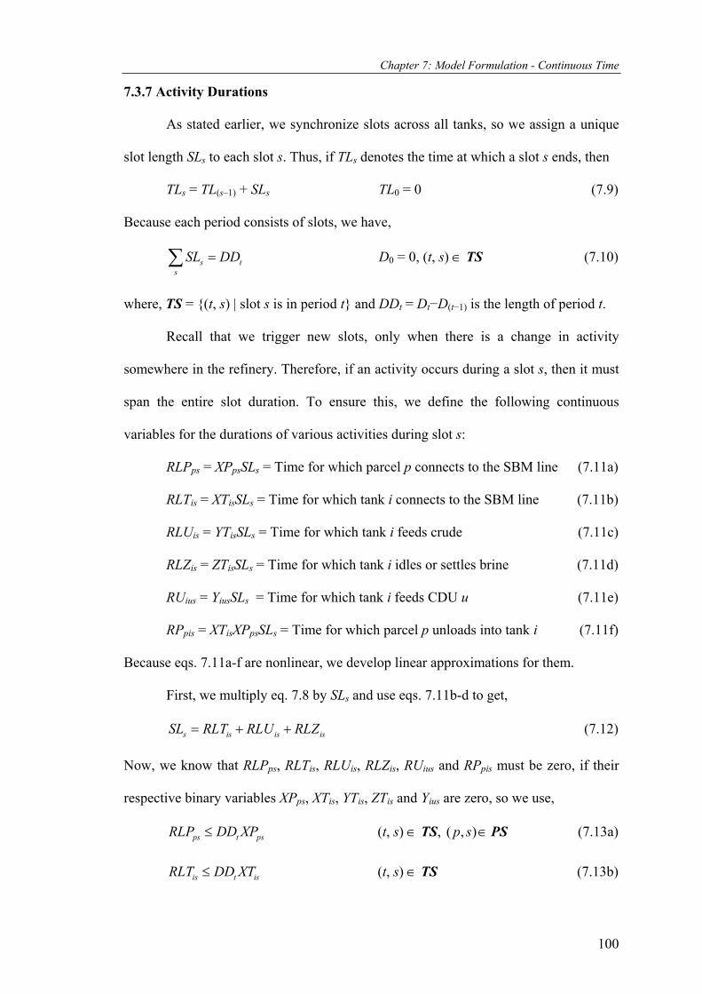
Chapter 7: Model Formulation - Continuous Time
7.3.7 Activity Durations
As stated earlier, we synchronize slots across all tanks, so we assign a unique
slot length SLs to each slot s. Thus, if TLs denotes the time at which a slot s ends, then
TLs = TL(s–1) + SLs TL0 = 0 (7.9)
Because each period consists of slots, we have,
s ts
SL DD=∑ D0 = 0, (t, s) ∈ TS (7.10)
where, TS = {(t, s) | slot s is in period t} and DDt = Dt−D(t−1) is the length of period t.
Recall that we trigger new slots, only when there is a change in activity
somewhere in the refinery. Therefore, if an activity occurs during a slot s, then it must
span the entire slot duration. To ensure this, we define the following continuous
variables for the durations of various activities during slot s:
RLPps = XPpsSLs = Time for which parcel p connects to the SBM line (7.11a)
RLTis = XTisSLs = Time for which tank i connects to the SBM line (7.11b)
RLUis = YTisSLs = Time for which tank i feeds crude (7.11c)
RLZis = ZTisSLs = Time for which tank i idles or settles brine (7.11d)
RUius = YiusSLs = Time for which tank i feeds CDU u (7.11e)
RPpis = XTisXPpsSLs = Time for which parcel p unloads into tank i (7.11f)
Because eqs. 7.11a-f are nonlinear, we develop linear approximations for them.
First, we multiply eq. 7.8 by SLs and use eqs. 7.11b-d to get,
s is is isSL RLT RLU RLZ= + + (7.12)
Now, we know that RLPps, RLTis, RLUis, RLZis, RUius and RPpis must be zero, if their
respective binary variables XPps, XTis, YTis, ZTis and Yius are zero, so we use,
ps t psRLP DD XP≤ (t, s) ∈ TS, ( , )p s ∈PS (7.13a)
is t isRLT DD XT≤ (t, s) ∈ TS (7.13b)
100

Chapter 7: Model Formulation - Continuous Time
is t isRLU DD YT≤ (t, s) ∈ TS (7.13c)
is t isRLZ DD ZT≤ (t, s) ∈ TS (7.13d)
RUius ≤ DDt Yius (i, u) ∈ IU, (t, s) ∈ TS (7.13e)
pis isp
RP RLT≤∑ (p, s) ∈ PS, (p, i) ∈ PI (7.14a)
pis psi
RP RLP≤∑ (p, s) ∈ PS, (p, i) ∈ PI (7.14b)
Then, we multiply eqs. 7.4, 7.5 and 7.8a-b by SLs to get,
ps sp
RLP SL≤∑ (p, s) ∈ PS (7.15)
is psi p
RLT RLP≤∑ ∑ (p, s) ∈ PS, (p, i) ∈ PI (7.16)
RLUis ≥ RUius (i, u) ∈ IU (7.17a)
ius isu
RU RLU≥∑ (i, u) ∈ IU (7.17b)
Lastly, to make RPpis and RUius equal slot length, when their respective activities take
place, we use,
RUius ≥ RLUis − DDt(1−Yius) (i, u) ∈ IU, (t, s) ∈ TS (7.18)
RPpis ≥ RLTis + RLPps − SLs (p, s) ∈ PS, (p, i) ∈ PI (7.19)
We can derive eqs. 7.14a-b and 7.19 as follows:
Define a 0-1 continuous variable Xpis as:
Xpis = { 1 if tank is receiving crude from parcel during slot 0 otherwise
i p s
Since a tank i can receive crude from parcel p, only if both the tank and the parcel are
connected to the SBM line (i.e., XTis = 1 and XPps = 1). In other words, Xpis = XPps
XTis. A linear approximation for this is given by,
pis isp
X XT≤∑ (p, s) ∈ PS, (p, i) ∈ PI (i)
pis psi
X XP≤∑ (p, s) ∈ PS, (p, i) ∈ PI (ii)
101
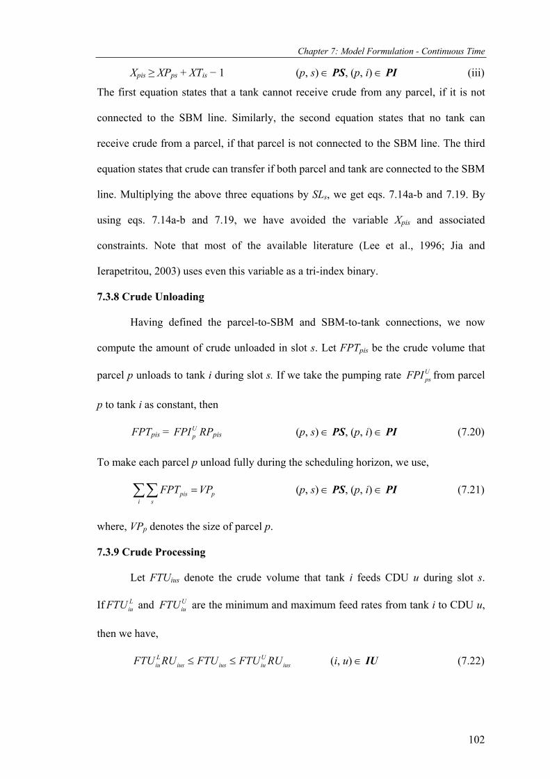
Chapter 7: Model Formulation - Continuous Time
Xpis ≥ XPps + XTis − 1 (p, s) ∈ PS, (p, i) ∈ PI (iii)
The first equation states that a tank cannot receive crude from any parcel, if it is not
connected to the SBM line. Similarly, the second equation states that no tank can
receive crude from a parcel, if that parcel is not connected to the SBM line. The third
equation states that crude can transfer if both parcel and tank are connected to the SBM
line. Multiplying the above three equations by SLs, we get eqs. 7.14a-b and 7.19. By
using eqs. 7.14a-b and 7.19, we have avoided the variable Xpis and associated
constraints. Note that most of the available literature (Lee et al., 1996; Jia and
Ierapetritou, 2003) uses even this variable as a tri-index binary.
7.3.8 Crude Unloading
Having defined the parcel-to-SBM and SBM-to-tank connections, we now
compute the amount of crude unloaded in slot s. Let FPTpis be the crude volume that
parcel p unloads to tank i during slot s. If we take the pumping rate from parcel
p to tank i as constant, then
UpsFPI
FPTpis = RPUpFPI pis (p, s) ∈ PS, (p, i) ∈ PI (7.20)
To make each parcel p unload fully during the scheduling horizon, we use,
pis pi s
FPT VP=∑∑ (p, s) ∈ PS, (p, i) ∈ PI (7.21)
where, VPp denotes the size of parcel p.
7.3.9 Crude Processing
Let FTUius denote the crude volume that tank i feeds CDU u during slot s.
If and are the minimum and maximum feed rates from tank i to CDU u,
then we have,
LiuFTU U
iuFTU
Liu ius ius iu iusFTU RU FTU FTU RU≤ ≤ U (i, u) ∈ IU (7.22)
102

Chapter 7: Model Formulation - Continuous Time
For individual crudes fed to CDUs, we define FCTUiucs as the amount of crude c fed
by tank i to CDU u during slot s. Then, the total crude amount FTUius that tank i feeds
CDU u during s is,
ius iucsc
FTU FCTU=∑ (i, u) ∈ IU, (i, c) ∈ IC (7.23)
where, IC = {(i, c) | tank i may hold crude c}. Because multiple tanks may feed a
CDU, the total feed FUus to CDU u during slot s is,
FUus = iusi
FTU∑ (i, u) ∈ IU (7.24)
This must be within the processing limits of CDU u:
SLLuFU s ≤ FUus ≤ SLU
uFU s (7.25)
where, and are the lower and upper limits on the processing rate of CDU u. LuFU U
uFU
In practice, the plant operation may know that a CDU cannot process a feed
with some extreme fractions of crudes. To impose such limitations, we use,
Lus cu iucs us cu
iFU xc FCTU FU xc≤ ≤∑ U (i, u) ∈ IU, (i, c) ∈ IC (7.26)
Similarly, the concentration of a key component may also be critical to the operation of
a CDU and must be within certain allowable limits. If xkkc is the fraction of a key
component k in crude c, then we respect these limits by using,
L Uku us iucs kc ku us
i cxk FU FCTU xk xk FU≤ ≤∑∑ , (i, u) ∈ IU, (i, c) ∈ IC (7.27)
7.3.10 Crude Balance
First, to identify the crude in parcel p, we define a set PC = {(p, c) | parcel p
carries crude c}. Using VCTics to denote the amount of crude c in tank i at the end of
slot s, we write a crude balance on tank i as,
( 1)( , ) ,( , ) ( , )
ics ic s pis iucsp c p i i u
VCT VCT FPT FCTU−∈ ∈ ∈
= + −∑ ∑PC PI IU
(i, c) ∈ IC (7.28)
103
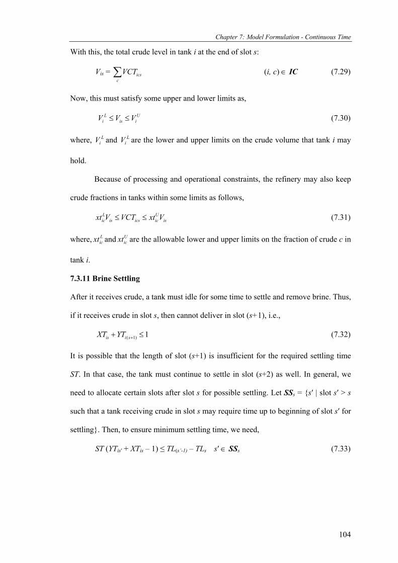
Chapter 7: Model Formulation - Continuous Time
With this, the total crude level in tank i at the end of slot s:
Vis = (i, c) ∈ IC (7.29) ∑c
icsVCT
Now, this must satisfy some upper and lower limits as,
V V (7.30) Li is V≤ ≤ U
i
U
where, V and V are the lower and upper limits on the crude volume that tank i may
hold.
Li
Li
Because of processing and operational constraints, the refinery may also keep
crude fractions in tanks within some limits as follows,
Lic is ics ic isxt V VCT xt V≤ ≤ (7.31)
where, and are the allowable lower and upper limits on the fraction of crude c in
tank i.
Licxt U
icxt
7.3.11 Brine Settling
After it receives crude, a tank must idle for some time to settle and remove brine. Thus,
if it receives crude in slot s, then cannot deliver in slot (s+1), i.e.,
( 1) 1is i sXT YT ++ ≤ (7.32)
It is possible that the length of slot (s+1) is insufficient for the required settling time
ST. In that case, the tank must continue to settle in slot (s+2) as well. In general, we
need to allocate certain slots after slot s for possible settling. Let SSs = {s′ | slot s′ > s
such that a tank receiving crude in slot s may require time up to beginning of slot s′ for
settling}. Then, to ensure minimum settling time, we need,
ST (YTis′ + XTis – 1) ≤ TL(s’-1) – TLs s′ ∈ SSs (7.33)
104
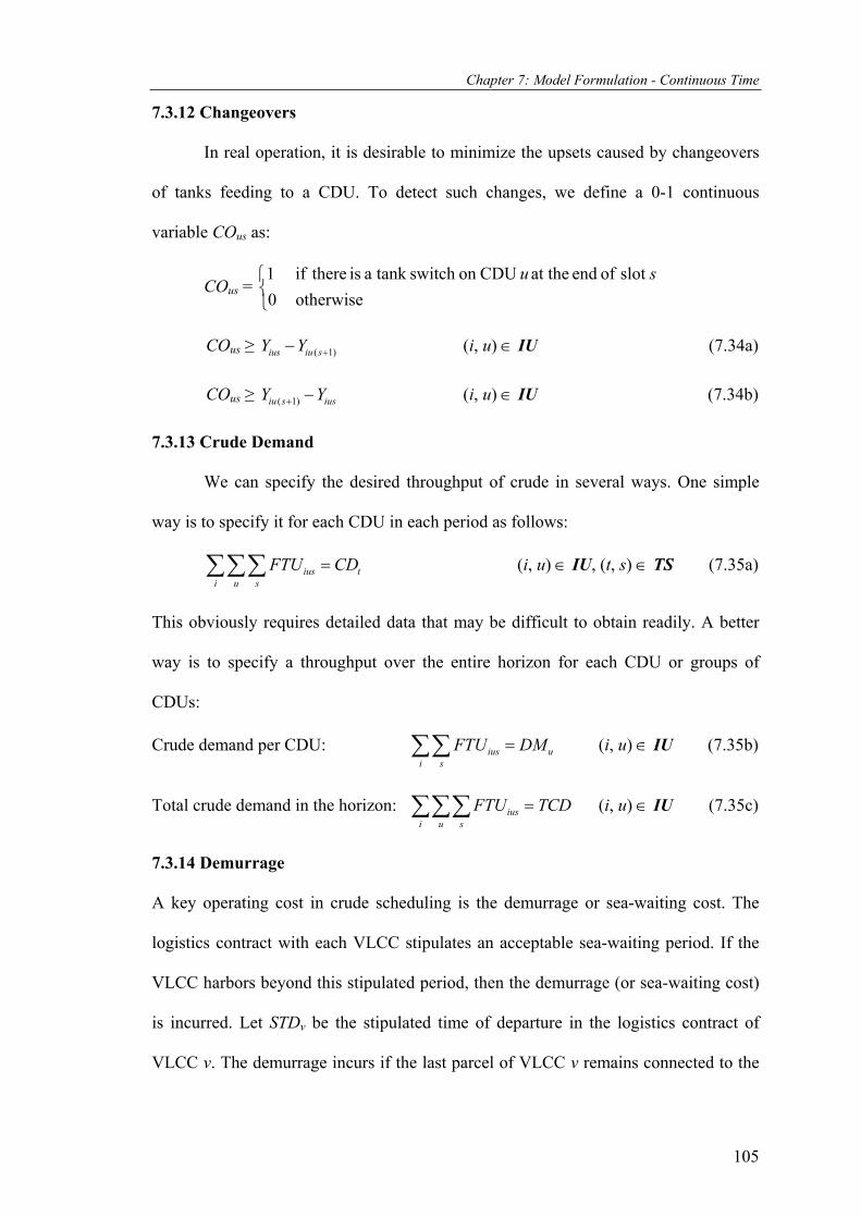
Chapter 7: Model Formulation - Continuous Time
7.3.12 Changeovers
In real operation, it is desirable to minimize the upsets caused by changeovers
of tanks feeding to a CDU. To detect such changes, we define a 0-1 continuous
variable COus as:
COus = otherwise
slot of end at the CDUon switch tank a is thereif01 su
Y
COus ≥ Y Y (i, u) ∈ IU (7.34a) ( 1)ius iu s+−
COus ≥ Y (i, u) ∈ IU (7.34b) ( 1)iu s ius+ −
7.3.13 Crude Demand
We can specify the desired throughput of crude in several ways. One simple
way is to specify it for each CDU in each period as follows:
ius ti u s
FTU CD=∑∑∑ (i, u) ∈ IU, (t, s) ∈ TS (7.35a)
This obviously requires detailed data that may be difficult to obtain readily. A better
way is to specify a throughput over the entire horizon for each CDU or groups of
CDUs:
Crude demand per CDU: ius ui s
FTU DM=∑∑ (i, u) ∈ IU (7.35b)
Total crude demand in the horizon: iusi u s
FTU TCD=∑∑∑ (i, u) ∈ IU (7.35c)
7.3.14 Demurrage
A key operating cost in crude scheduling is the demurrage or sea-waiting cost. The
logistics contract with each VLCC stipulates an acceptable sea-waiting period. If the
VLCC harbors beyond this stipulated period, then the demurrage (or sea-waiting cost)
is incurred. Let STDv be the stipulated time of departure in the logistics contract of
VLCC v. The demurrage incurs if the last parcel of VLCC v remains connected to the
105

Chapter 7: Model Formulation - Continuous Time
SBM line beyond STDv. If VLCC v arrives at the start of period t and its demurrage or
sea-waiting cost is SWCv per unit time, then the demurrage incurred is:
DCv ≥ SWCv[TLs – STDvXPps – Dt(1–XPs)] (t, s) ∈ TS, (p, v) ∈ PV (7.36)
where, PV = {(p, v) | parcel p is the last parcel in VLCC v}.
7.3.15 Objective
We use total gross profit as the scheduling objective. We define this as the total
marginal profit (netback) from crudes minus the operating cost. The former is simply
the value of products minus the purchase cost of crude. Since the product yields vary
with crudes and CDUs, we define CPcu as the marginal profit ($ per unit volume) for
crude c processed in CDU u. Note that the marginal profit does not include any
operating costs.
The operating costs include the changeover costs, the demurrage and the
penalty for under-running the crude safety stock. As noted earlier, a change in the feed
composition (tanks) to a CDU is called a changeover. A changeover lasts a few hours
and leads to off-spec products or slops during the transition. In other words, every
changeover incurs some cost to the refinery and is undesirable. Let COC be the cost
per changeover. The refinery may wish to keep a minimum crude inventory SSt at the
end of period t. We call this the desired safety stock of crude. To prevent the crude
inventory from dropping below this level, we assign a penalty SSPt ($ per unit volume)
for period t for under-running the crude safety stock. Based on the above discussion,
we compute the operating costs and obtain the total gross profit as,
Profit = iucs cu v us ti u c s v u s t
FCTU CP DC COC CO SC− − −∑∑∑∑ ∑ ∑∑ ∑ (7.37)
SCt ≥ SSPt(SSt – ) (t, s) ∈ LAST (7.37a) isi
V∑
where, LAST = {(t, s) | slot s is the last slot in period t}.
106

Chapter 7: Model Formulation - Continuous Time
107
This completes our continuous-time formulation (eqs. 7.1-7.37a) for a refinery
with one SBM line. A coastal refinery may use a single jetty to receive small ships
carrying single crude parcels. Since the pipeline connecting the jetty to the refinery
tank farm usually has negligible volume, we can ignore its crude holdup. This makes
the SBM parcels disappear from our formulation and we can use the proposed
formulation as is to handle a single jetty by treating the individual marine vessels as
single-parcel VLCCs.
As discussed in chapter 5, the discrete time MILP model experiences the non linearity
issue inherent to crude mixing in the storage tanks. The continuous time model too
suffers from this problem and leads to a solution with composition discrepancy. In the
next chapter we develop a solution algorithm for continuous time model using an
approach identical to that developed for discrete model in chapter 5.

Chapter 8
SOLUTION ALGORITHM – Continuous Time
8.1 Introduction
The blending of crudes in tanks makes the crude scheduling problem inherently
nonlinear. The proposed linear formulation is thus an approximation. The linear crude
balance constraints (Eqs. 7.22-7.27) allow the optimizer to push arbitrary amounts of
individual crudes to a CDU rather than in the proportions dictated by the tank
composition. This results in a disproportionate delivery of crudes to CDUs. For a
discrete-time formulation, chapter 5 presented a novel iterative strategy to eliminate
this problem. In the next section, we modify this strategy to suit the proposed
continuous-time approach without solving any nonlinear problem.
8.2 Description
To avoid disproportionate delivery, we must use the correct nonlinear constraint
FCTUiucs = fics FTUius, where fics is the fraction of crude c in tank i at the end of slot s.
We now devise an iterative strategy that solves a series of MILPs of reducing size and
complexity to obtain a near-optimal solution with no discrepancy in the crude
composition delivered to a CDU.
Observe that every tank has blocks of contiguous slots during which its
composition does not change, because it receives no crude. For such a block, if we
knew that constant composition (fic), then the nonlinear equation (FCTUiucs = fic
FTUius) becomes linear. Solving an MILP with these constraints would yield a solution
with no composition discrepancy. Thus, for each tank, we divide all slots into two
distinct blocks: one for which we know the tank compositions, and the other for which
108

Chapter 8: Solution Algorithm-Continuous Time
we do not. For the former, we use the exact linear constraints (FCTUiucs = fic FTUius)
and for the latter, we use the linear approximations as in our formulation. Furthermore,
note that a tank’s composition changes, only when it receives crude from a parcel or
another tank, otherwise not. During most slots, the tank will receive nothing; hence its
composition will be constant. However, we must know that composition to make the
nonlinear flow constraints linear. To this end, our knowledge of the initial
compositions of tanks proves useful. Because we know the initial composition in each
tank, we can identify one initial block of slots for which the composition is constant
and known. The length of this block will vary from tank to tank and it could be as
short as just one slot for some tanks. However, this at least provides a start for our
algorithm. As a first try, we use the exact linear constraints for these first blocks of
slots and linear approximations for the remaining slots and solve the MILP. This gives
us a solution that has no composition discrepancy at least for the first block of slots on
each tank. It also gives us the compositions in all tanks at the end of each slot in each
block. We now identify the first common block of slots for which we know the
compositions in all tanks. We freeze the schedule until the end of that block, and repeat
the entire procedure for scheduling the remaining slots. In other words, we now solve
another scheduling problem with a reduced horizon. In this manner, we get
progressively longer and longer partial schedules, free of composition discrepancies,
by solving a series of MILPs, until we have the complete schedule. We now describe
the algorithm in full detail.
8.3 Step-wise Procedure
At each iteration of our algorithm, we divide the NS slots into two sets. Set 1
includes all slots with s ≤ s* for some s*, and set 2 the rest. The schedule (or all
variables Yius, XPps, XTis ,FTUius, FCTUiucs, etc. in the MILP) for slots in set 1 is (are)
109

Chapter 8: Solution Algorithm-Continuous Time
fixed based on previous iterations. However, the MILP variables for slots in set 2 are
free. From the schedule for set 1, we know the tank compositions at the end of slot s*.
Let fic denote the fraction of crude c in tank i at s = s*. Then, our iterative algorithm
proceeds as follows:
1. Set s* = 0.
2. From the fixed schedule for s ≤ s*, compute fic for each tank i as fic = VCTics* / Vis*
using the known information (VCTics* and Vis*).
3. For each tank i, identify the latest slot > s*is * such that its composition is fic for all
slots s* < s ≤ . We do this as follows. Let p′ denote the last parcel that was
unloaded (to any tank) before s
*is
* and p″ denote the earliest parcel (p″ ≥ p′) that tank
i can possibly receive after s*. Two possibilities exist, namely that p′ has finished
unloading or p′ has partially unloaded.
First, consider that p′ has fully unloaded, i.e. XLp′s* = 1. If parcel p″ does not
exist, then = NS. If both p′ and p″ belong to the same VLCC, then = s*is *
is *+ (p″−
p′). This is because we need at least one slot to unload a parcel. If p″ belongs to a
different vessel, then = ETU*is p″, which is the slot in which p″ can possibly start
unloading. Next, consider that p′ has partially unloaded. Then, = s*is * + (p″−p′) + 1
for an i that cannot receive crude from p′ and = s*is *+1 for an i that can do so.
4. Add the constraint, FCTUiucs = ficFTUius, for s* < s ≤ in the MILP and solve. *is
5. Fix the MILP variables for s* < s ≤ mini[ ]. Set s*is * = mini[ ]. If s*
is * = NS, then
terminate, otherwise go to Step 2.
8.4 Discussion
Note that the size and complexity of the MILP in our algorithm reduce progressively
by at least one slot at each iteration. However, for periods in which no VLCC arrives,
110

Chapter 8: Solution Algorithm-Continuous Time
111
the size and complexity reduce by one full period. Because our approach fixes MILP
variables based on a solution from linear approximation, it cannot guarantee an optimal
solution. However, considering the fact that even solving the approximate MILP is a
challenging problem, our approach is quite attractive because it does not require
solving MINLPs or NLPs and gives near-optimal schedules in reasonable time. When
the scheduling objective does not involve crude compositions (minimizing operating
cost as objective instead of profit), then our algorithm guarantees an optimal objective
value right in the first MILP, although further iterations are required to correct the
composition discrepancy. For large and complex problems, solving even the MILP to a
zero gap is compute-intensive; hence we may have to target a small optimality gap for
the first few iterations. As iterations proceed in our algorithm, the problem size
reduces. This reduces the computation time drastically and allows us to target even
smaller relative gaps in progressive iterations. For example, if a problem has NS = 30,
then we can use a relative gap of 5% for the first few iterations and 0% for the rest,
when the MILP becomes easier to solve.
In the next chapter, we illustrate our methodology on several examples derived from a
local refinery (SRC Singapore). In order to maintain confidentiality, we used different
set of data but kept the nature of problem identical, employed similar operating rules
Chapter 9
COMPUTATIONAL RESULTS
9.1 EXAMPLES
We illustrate our methodology using three examples. We take a refinery with 8 tanks
(T1-T8), 3 CDUs (CDU1-CDU3) and two classes (Class1 & Class2) of crudes. Tanks
T1, T6, T7, T8 and CDU3 handle Class1 crudes, while the rest handle Class2 crudes.
For all Examples 1 to 3, Table 8.1 gives the tanker arrival details, crude demands and
key component concentration limits on CDUs. Table 8.2 gives the initial crude levels
in tanks and tank capacity details. Table 8.3a gives the economic data and limits on
crude transfer amounts. Table 8.3b provides information about crudes, their marginal
profits and key component concentrations. As mentioned earlier, detailed model
information and problem data for the literature (Joly et al., 2002; Jia and Ierapetritou,
2003; Magalhães and Shah, 2003) on continuous formulations are not available, so we
compare continuous time approach with the discrete-time approach developed and
explained earlier. It is important to do this, because the issue of which approach
(continuous-time or discrete-time) is better for this problem is yet to be resolved
conclusively. However, there is some difficulty in comparing the schedules and profits
from the two approaches on the same footing because of the following reasons.
1) In a discrete-time model, demurrage counts for multiples of the uniform slot, while
in a continuous-time model, its counting is on a per unit time basis and thus
accurate.
2) Violation of minimum safety stock is checked and penalized at every slot in a
discrete-time model, while it is done at event points (periods) only in a continuous-
112
Chapter 9: Computational Results
time model. This is because an inventory penalty depends on time as well and
variable-length slots would result in a nonlinear formulation.
3) A discrete-time model allows amount transferred to a tank in a period to vary
between some lower and upper limits. This makes us the transfer rate flexible. In a
continuous-time model, however, the transfer rate is fixed and the amount depends
on the slot length. It would be desirable to use the maximum possible transfer rate
to minimize demurrage, so a fixed transfer rate is closer to real practice, but a
variable one may prove prudent in some situations.
4) In the discrete time approach, we considered even a change in the tank-to-CDU
flow as a changeover, when two tanks are feeding to one CDU, as such a change
alters feed composition. A discrete model has the advantage of avoiding such
changeovers by forcing the flows from respective tanks to be constant in
contiguous periods. In the proposed continuous model, a comparison of flow rates
in consecutive slots introduces a nonlinearity that forces the algorithm to adjust the
flow by generating MILP at every slot and making the problem compute intense.
In fact, it is easier to adjust the flow rates to avoid such changeovers, after we get
the final schedule. Therefore, we avoid the flow matching constraints in both
models and use the changeover definition mentioned in this paper for a fair
comparison of both models.
For the three examples, we used CPLEX 7.0 solver within GAMS on a SUN enterprise
250 server using SUN OS 5.7, Single Ultra SPARC II 400 MHz Processor and 2 GB
RAM. Tables 9.4 and 9.5 give the model statistics and performances respectively for
all examples. We see (Table 9.5) that the continuous-time formulation uses more
variables and constraints, but fewer binary variables.
113

Chapter 9: Computational Results Chapter 9: Computational Results
114
114
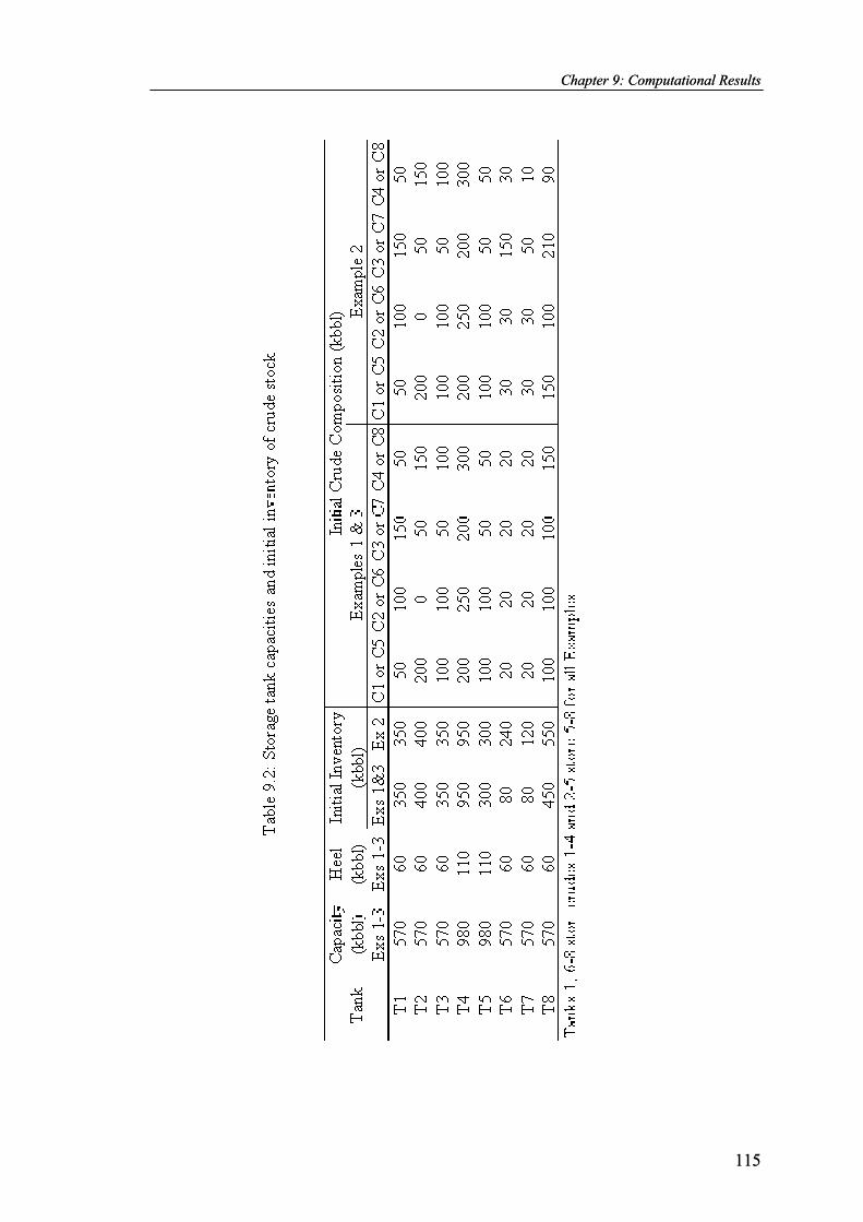
Chapter 9: Computational Results Chapter 9: Computational Results
115
115

Chapter 9: Computational Results Chapter 9: Computational Results
116
116

Chapter 9: Computational Results
117
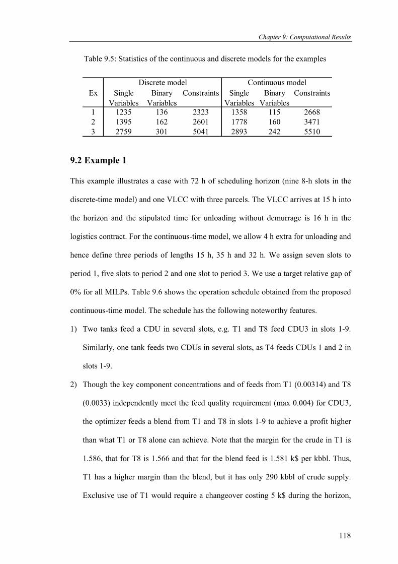
Chapter 9: Computational Results
Ex Single Binary Constraints Single Binary ConstraintsVariables Variables Variables Variables
1 1235 136 2323 1358 115 26682 1395 162 2601 1778 160 34713 2759 301 5041 2893 242 5510
Continuous modelDiscrete model
Table 9.5: Statistics of the continuous and discrete models for the examples
9.2 Example 1
This example illustrates a case with 72 h of scheduling horizon (nine 8-h slots in the
discrete-time model) and one VLCC with three parcels. The VLCC arrives at 15 h into
the horizon and the stipulated time for unloading without demurrage is 16 h in the
logistics contract. For the continuous-time model, we allow 4 h extra for unloading and
hence define three periods of lengths 15 h, 35 h and 32 h. We assign seven slots to
period 1, five slots to period 2 and one slot to period 3. We use a target relative gap of
0% for all MILPs. Table 9.6 shows the operation schedule obtained from the proposed
continuous-time model. The schedule has the following noteworthy features.
1) Two tanks feed a CDU in several slots, e.g. T1 and T8 feed CDU3 in slots 1-9.
Similarly, one tank feeds two CDUs in several slots, as T4 feeds CDUs 1 and 2 in
slots 1-9.
2) Though the key component concentrations and of feeds from T1 (0.00314) and T8
(0.0033) independently meet the feed quality requirement (max 0.004) for CDU3,
the optimizer feeds a blend from T1 and T8 in slots 1-9 to achieve a profit higher
than what T1 or T8 alone can achieve. Note that the margin for the crude in T1 is
1.586, that for T8 is 1.566 and that for the blend feed is 1.581 k$ per kbbl. Thus,
T1 has a higher margin than the blend, but it has only 290 kbbl of crude supply.
Exclusive use of T1 would require a changeover costing 5 k$ during the horizon,
118

Chapter 9: Computational Results
because the asking rate for crude throughput is 300 kbbl. The optimizer makes up
the shortfall of 10 kbbl by using some crude from T8 and avoids the changeover to
achieve an increase in profit of 3.85 k$. This aptly illustrates (a) the trade-off
between margin and changeover and (b) the judicious use of available resources to
minimize changeovers.
In this example, sufficient ullage for crude receipt and adequate supply for
crude are available. Thus, no changeover takes place and other features of our model
such as the brine-settling time, though inherently taken care of, are absent in the
schedule, as tanks that receive crude never deliver.
To compare our continuous model with the discrete model, we obtain two
solutions using the latter. In Case1, we allow two parcel-to-tank transfers in one slot,
while three in Case2. Table 9.6 also gives the schedule from the discrete model for
Case2. Apart from the timing differences that arise due to the different arrival times
(Table 9.1) in the two models, the schedules from the continuous and discrete models
are essentially the same. As expected, Case1 assigns 24 h for crude unloading, while
Case2 assigns 16 h. Thus, in terms of time utilization, Case2 produces a schedule
closer to the one from the continuous model. All schedules have the same profit,
because the receiving tanks are not required to feed CDUs. However, the discrete
model for Case2 seems 28% faster than the continuous model (Table 9.6). Note (Table
9.4) that Case1 solves significantly slower than Case2. In addition, the continuous
model needs five iterations as compared to three for Case2. However, this does not
affect the profit, because the tanks whose compositions change do not feed CDUs.
119

Chapter 9: Computational Results
120
Chapter 9: Computational Results
9.3 Example 2
In this example, we use a horizon of 80 h (ten 8-h slots in the discrete model) and one
VLCC with three parcels. In this example, we consider a situation where the ullage is
sparsely distributed among the tanks, parcel sizes are bigger and key component
concentration limits on feeds to CDUs are tighter. The VLCC arrives at 8 h and the
plant has 32 h to unload its parcels without incurring demurrage. We allow eight hours
more for unloading in our continuous model and use three periods of lengths 8 h, 40 h
and 32 h. We assign one slot to period 1, seven to period 2 and one to period 3. We
target a relative gap of 0.5% for the first MILP and 0% for all others. Table 9.7 shows
the operation schedule generated by the continuous model with the following salient
features:
1) The model ensures the required time for brine settling/removal between crude
receipt and delivery. For instance, T1 receives crude from the SBM parcel and the
first parcel of the VLCC during slots 2 and 3 and then idles for brine removal
during slots 4 and 5. Slots 4 and 5 have a combined length of 14.6 h, which
exceeds the required settling time of 8 h. Similarly, T6, after receiving crude from
parcel 2 in slot 4, allows 8 h of settling in slot 5 before feeding CDU3.
2) Although T2 with a key component concentration of 0.0108 can alone feed CDU2
(max 0.012), the optimizer feeds a blend of T2 and T4. This is because T4 has a
higher margin, but T4 with a key component concentration of 0.01257 alone
cannot meet the feed quality requirement of 0.012. By using a blend, the optimizer
also avoids a changeover.
3) The schedule also exhibits other features mentioned earlier in Example 1 such as
single tank (T4) feeding multiple CDUs (1 and 2), and two tanks (T1 and T6)
feeding one CDU (CDU3).
121
Chapter 9: Computational Results
We again compare the continuous-time solution with two solutions from the
discrete model. As before, Case1 allows two parcel-to-tank transfers in one slot, while
Case2 allows three. Table 9.7 describes the schedule for Case2. Again, Case2 schedule
is closer to the continuous-time schedule, but it gives a greater profit (1771.7 vs.
1766.4 in Table 9.4). Case1 uses five slots for unloading, while Case2 uses only four.
Case2 also solves 31.8% faster than the continuous model. Reasons for the latter’s
faster performance are multiple parcel transfers in a single slot. They help reduce the
MILP iterations. By allowing three transfers per slot, the Case2 model has longer
constant composition zones that allow the optimizer to select better blends and
minimize changeovers. On the other hand, the continuous model uses shorter blocks of
constant composition, which limits the blend adjustments and can increase
changeovers. However, longer horizons mean more binary variables in the discrete
model, making the problems more difficult, while the continuous model should require
fewer slots. That should make the continuous model faster for the bigger problems, as
the slots are of variable lengths. To demonstrate this, we use the next example.
9.4 Example 3
We use 160 h of horizon (Twenty 8-h slots in the discrete model) and two VLCCs with
three parcels each. VLCC-1 arrives at 15 h and VLCC-2 at 100 h. The stipulated
berthing time for both VLCCs is 20 h. Allowing 5 h extra for unloading, we define five
periods with lengths 15 h, 25 h, 60 h, 25 h and 35 h. We assign one, five, two, five and
two slots to periods 1 through 5 respectively. We use a target relative gap of 1% for the
first MILP and 0.5% for the rest. Table 8 shows the operation schedule from the
continuous model. Note that:
1) Though we used 15 slots, the optimizer needed only 14. Slot 8 in period 3 proved
extra and its length is zero. Slots 7 and 8 have identical activities on tanks.
122

Chapter 9: Computational Results
123

Chapter 9: Computational Results
124

Chapter 9: Computational Results
125
2. A tank may receive over several slots. For instance, T2 receives crude from parcels
5-7 during slots 9, 10 and 11. It then settles and removes brine during slots 12 and
13, before feeding CDU2 in slot 14.
3. The schedule also supports other features illustrated in the previous examples.
We use the same two cases for the discrete model as in the previous examples.
Table 9.8 also presents the schedule for Case2. Case2 gives a slightly higher profit
than the continuous model, but as expected, the latter is slightly faster than the former.
From Table 9.4, we see that the solution times decrease drastically for the
discrete models after the first iteration for all three examples. However, the same is not
true for the continuous model. In addition, the solution time decreases, as we allow
more parcels to transfer in a slot in the discrete model. Another point to note is the
huge difference in the solution times for the first iterations between the discrete and
continuous models.
9.5 CONCLUSION
This work presents the first complete, continuous-time MILP model for short-term
scheduling of crude operations of a refinery with an SBM pipeline. We used three
examples to show the efficacy of model and solution algorithm to solve the difficult
problem in reasonable time. In addition to accounting for real practices such as
multiple tanks feeding one CDU, one tank feeding multiple CDUs, unloading via SBM
pipeline, brine settling, etc., the proposed algorithm gives near-optimal schedules
without solving a single NLP or MINLP as illustrated through three industrial
problems. A direct head-to-head comparison between the two competing formulations
(discrete, continuous) reveals that the proposed continuous-time approach should out
do the discrete-time one for problems with longer horizons.
Chapter 10
CONCLUSIONS AND RECOMMENDATIONS
10.1 Conclusions
In part I of this work, a discrete-time MILP model that allows some tasks to begin even
at intermediate points in a period and a novel solution algorithm that shows no
composition discrepancy were developed for the scheduling of crude oil operations in
a refinery. In addition to including several real features such as multiple tanks feeding
one CDU, one tank feeding multiple CDUs, SBM pipeline, brine settling, tank-to-tank
transfers etc., the proposed model uses fewer binary variables and is different from and
superior (both in terms of efficiency and quality of solutions) to those reported in
previous work. The proposed model considers configurationally different crude oil
unloading facilities and uses different set of constraints for each facility. The main
feature of our algorithm is that it solves the oil quality, transfer quantity, tank
allocation and oil blending issues simultaneously without solving a single NLP or
MINLP. The proposed approach helps quicker and near-optimal decision making in
refinery operations and handles problems with up to 14 days. Longer horizon problems
increase the number of binary decisions and problem size, making it highly compute
intensive. Though some of continuous time features were incorporated in this model,
we had to use increased optimality gap to get a quicker solution. Alternative
methodology was to consider an inherent continuous time model to find a solution to
such problems. Despite being the Holy Grail, continuous-time formulations are far
behind their discrete counterparts in solving the complex problem of scheduling short-
126

Chapter 10: Conclusions and Recommendations
term crude operations in an oil refinery. In fact, none of the reported continuous-time
formulations has succeeded in addressing the problem satisfactorily.
Part II of this work, presents the first complete, continuous-time MILP model for
short-term scheduling of crude operations of a refinery with an SBM pipeline. Our
novel model uses fewer binary variables than the existing ones and our solution
algorithm eliminates composition discrepancy. In addition to accounting for real
practices such as multiple tanks feeding one CDU, one tank feeding multiple CDUs,
unloading via SBM pipeline, brine settling, etc., the proposed algorithm gives near-
optimal schedules without solving a single NLP or MINLP as illustrated through three
industrial size problems. A direct head-to-head comparison between the two competing
formulations reveals that the proposed continuous-time approach should outdo the
discrete-time one for problems with longer horizons. Although the latter currently
appears to be better for smaller and more complex problems, we expect that, with
future improvements, the superiority of the former would be clearly established. Other
exact methods based on mathematical programming prove to be computationally very
expensive even for small problems. From a comprehensive scheduling perspective, the
new methodology developed shows promising results both in terms of efficiency and
quality of solutions
Further work is also needed to solve the challenges of composition discrepancy, longer
scheduling horizons, and more complex operational aspects, all with full optimality in
reasonable time. To this end, we believe that this work is a significant step in the right
direction.
10.2 Recommendations
The developed model and algorithm allow us to solve the issues of crude feed quality;
crude transfer quantity and the tank allocations in one go but provide a near optimal
127

Chapter 10: Conclusions and Recommendations
128
solution for the crude scheduling problem. One needs to look into a different approach
than that is presented here for finding a better solution or optimal solution. The
developed approach imitates a roll forward approach and always corrects the schedule
for any composition discrepancy and proceeds further. At present, we had concluded
that the present approach produces a feasible solution if one exists based on evaluation
of our approach on various examples. We did not thoroughly examine all the possible
infeasibilities associated with our approach. Thus there is further scope and need to
explore the infeasibilities (if any) associate with the present approach. Another area of
improvement for this problem can be use of some better heuristics. Application of
heuristics reduces the complexity of the problem and may facilitate a quicker and good
feasible solution to the problem.
The developed model can be easily extended to incorporate the product properties, cut
properties that are nonlinear in relationship but respective property indexes are linear
in blending. The present formulation assumes that key component limits on crude feed
determine the product pattern and quality. Using index relationships, we can easily
extend the present formulation to adjust the crude feed based on the product qualities
and quantities. Crude oil scheduling is first part of overall refinery operations
scheduling. Developing the other two parts namely hydraulic scheduling, product
blending & distribution scheduling, integrating all three parts and providing a user
interface should be the last stage of extension to this problem.

REFERENCES
1. Applequist, G., O. Samikoglu, J. Pekny and G. V. Reklaitis. Issues in the use,
Design and Evolution of Process Scheduling and Planning Systems, ISA
Trans., 36(2), pp.81-121. 1997
2. Alle, A. and J.M. Pinto, Mixed-Integer Programming Models for the
scheduling and Operational Optimization of Multiproduct Continuous Plants.
Ind. Eng. Chem. Res., 41, pp.2689-2704. 2002.
3. Ballintjin, K. Optimization in Refinery Scheduling: Modeling and Solution. In
T.A. Ciriani, & R.C.Leachman, Optimization in Industry, Vol.3, pp.191-199,
Wiley: New York. 1993.
4. Bodington, C. E. Inventory management in blending optimization: use of
nonlinear optimization for gasoline blends planning and scheduling, ORSA /
TIMS National Meeting, San Francisco (CA). 1992.
5. Bodington, C. E. Planning, scheduling, and integration in the process
industries, McGraw Hill: New York. 1995.
6. Bodington, C. E. and T. E. Baker. A History of Mathematical Programming in
the Petroleum Industry. Interfaces, 20(4), pp.117-127, July-August, 1990.
7. Cerda, J., G. P. Henning and I. E. Grossmann. A Mixed-Integer Linear-
Programming Model for Short-Term Scheduling of Single-Stage Multiproduct
Batch Plants with Parallel Lines, Ind. Eng. Chem. Res, 36(5), pp.1695-1707.
1997.
8. Chi-Wai Hui and Avaneesh Gupta. A Bi-index Continuous-Time Mixed-
Integer Linear Programming Model for Single-Stage Batch Scheduling with
Parallel Units. Ind. Eng. Chem. Res., 40, pp.5960-5967. 2001.
129

References
9. Coxhead, R. E. Integrated Planning and Scheduling Systems for the Refining
Industry. In T.A. Ciriani, & R.C.Leachman, Optimization in Industry, Vol.2,
pp.185-199.: Wiley: New York. 1993.
10. Glismann, K and G. Gruhn. Short-term Scheduling and Recipe Optimization of
Blending Processes. Comput. Chem. Eng., 25, pp.627-634. 2001.
11. Jia, Z. and M.G. Ierapetritou. Mixed-Integer Linear Programming Model for
Gasoline Blending and Distribution Scheduling. Ind. Eng. Chem. Res., 42,
pp.825-835. 2003.
12. Jia, Z. and M.G. Ierapetritou. Efficient Short-term Scheduling of Refinery
Operation Based on Continuous Time Formulation. FOCAPO, pp. 327-330.
2003a.
13. Jia, Z., M.G. Ierapetritou and Jeffrey D. Kelly. Refinery Short-Term
Scheduling Using Continuous Time Formulation: Crude-Oil Operations. Ind.
Eng. Chem. Res., 42, pp.3085-3097. 2003b.
14. Joly, M., L.F.L. Moro and J.M. Pinto. Planning and Scheduling for Petroleum
Refineries using Mathematical programming, Brazilian Journal of Chemical
Engineering, 19(2), pp. 207-228. 2002.
15. Karimi, I. A. and C. M. McDonald. Planning and Scheduling of Parallel Semi
continuous Processes. 2. Short-term Scheduling, Ind. Eng. Chem. Res., 36,
pp.2701-2714. 1997.
16. Kelly, J. D. Chronological Decomposition Heuristic for Scheduling: A divide
& Conquer Method. http://www.dashoptimization.com/pdf/cdhmilpv2.pdf.
March 2002.
130

References
17. Kelley, J. D., and J. F. Forbes. Structured Approach to Storage Allocation for
Improved Process Controllability, AIChE Journal, 44(8), pp.1832 -1840. 1998.
18. Kelley, J.D., and J.L. Mann. Crude-Oil Blend Scheduling Optimization: An
Application with Multi-Million Dollar Benefits,
‘http://www.acs.honeywell.com/ichome/Doc/0/GRUFIK9GRI6KR3VCOGKU
694A28/SchedOptim.pdf’. (2002)
19. Kelley, J. D. and J. L. Mann. Crude-Oil Blend Scheduling Optimization: An
Application with Multi-Million Dollar Benefits - Part 1, Hydrocarbon
Processing, 82(6), pp.47. 2003a.
20. Kelley, J. D., and J. L. Mann. Crude-Oil Blend Scheduling Optimization: An
Application with Multi-Million Dollar Benefits - Part 2, Hydrocarbon
Processing, 82(7), pp.xx. 2003b.
21. Kondili, E., C. C. Pantelides and R. W. H. Sargent. A General Algorithm for
Short-term Scheduling of Batch Operations- I. MILP Formulation, Computers
Chem. Eng., 17(2), pp.211-227. 1993.
22. Lamba, N. and I.A.Karimi. Scheduling Parallel Production Lines with
Resource Constraints-1.Model Formulation, Ind. Eng. Chem. Res., 41, pp.779-
789. 2002.
23. Lamba, N. and I.A.Karimi. Scheduling Parallel Production Lines with
Resource Constraints- 2. Decomposition Algorithm, Ind. Eng. Chem. Res., 41,
pp.790-800. 2002
131

References
24. Lee, H., J.M. Pinto, I.E. Grossmann and S. Park. Mixed-Integer Programming
Model for Refinery Short term Scheduling of Crude oil unloading with
Inventory Management, Ind. Eng. Chem. Res. 35, pp.1630-1641. 1996.
25. Li, W., C. W. Hui, Ben Hua, and T. Zhongxuan. Scheduling Crude Oil
Unloading, Storage, and Processing, Ind. Eng. Chem. Res., 41, pp.6723-6734.
2002.
26. Lim May Fong, Optimal Scheduling of Single Stage Batch/Semi continuous
Processes with Parallel Production Units and Multiple Orders. M. Engg.
Thesis, National University of Singapore. 2002
27. Magalhães, M. V., L. F. L Moro, P. Smania, M. K. Hassimotto, J. M. Pinto and
G.J. Abadia. SIPP-A solution for refinery scheduling. NPRA computer
conference, Nov 16-18, San Antonio, TX. 1998.
28. Magalhães, M.V. and N. Shah. Crude Oil Scheduling, FOCAPO, pp. 323-326.
2003.
29. Manne, A.S. Scheduling of Petroleum Operations; Harvard University Press:
Cambridge, MA, 1956.
30. Moro, L.F.L., A.C. Zanin and J.M. Pinto. A Planning model for refinery diesel
production, Comput. Chem. Eng., 22 (S), pp.S1039 – S1042. 1998.
31. Pantelides, C. C. Unified Framework for Optimal Process Planning and
Scheduling. In Proc. 2nd Conf. on the ‘Foundations of Comp. Aided Proc. Op.’
(FOCAPO'94), CACHE Corp., pp.253-274, 1994.
32. Pelham, R. and C. Pharris. Refinery operations and control: a future vision,
Hydrocarbon Processing, 75 (7), pp.89-94. 1996.
33. PIMS System Reference, version 11.0; AspenTech, Inc, Cambridge, MA, 1999
132

References
34. Pinto J.M and Joly M. Mixed Integer programming techniques for the
scheduling of fuel oil and asphalt production. ESCAPE-10, pp.1063-1068.
2000.
35. Pinto J.M and L.F.L. Moro. A Mixed Integer Model for LPG Scheduling.
ESCAPE-10, pp.1141-1146. 2000.
36. Pinto, J. M., M. Joly and L. Moro. Planning and scheduling models for refinery
operations, Comput. Chem. Eng., 24, pp.2259-2276. 2000.
37. Pinto, J. M. and I. E. Grossmann. Optimal Cyclic Scheduling of Multistage
Continuous Multiproduct Plants. Comput. Chem. Eng., 18(9), pp.797-816.
1994.
38. Quesada, I. And I. E. Grossmann. Global Optimization of Bilinear Process
Networks with Multicomponent Flows. Comput. Chem. Eng., 19(12), pp.1219-
1242. 1995.
39. RPMS (Refinery and Petrochemical Modeling System)-A system description,
Bonner & Moore Management Science, 2727 Allen Parkway, Suite 1200,
Houston, TX 77019. 1979.
40. Ramage, M.P. The petroleum industry of the 21stcentury. FOCAPO,
Snowmass, CO. 1998.
41. Reklaitis, G. V. Perspectives on Scheduling and Planning of Process
Operations. Proc.4th International Symposium in Process Systems Eng.,
Montebello, Canada. 1991.
42. Reklaitis, G. V. Overview of scheduling and planning of batch process
operations. NATO advanced study institute-Batch Process Systems
Engineering, Antalya, Turkey. 1992.
133
References
43. Rippin, D. W. T. Batch Process Systems Engineering: a Retrospective and
Prospective Review. Comput. Chem. Eng., S17, pp.S1-S13. 1993.
44. Rejowski, Jr., R., and J. M. Pinto. Scheduling of a multi-product pipeline
system, Comput. Chem. Eng., 27, pp.1229-1246. 2003.
45. Sahinidis, N. V. and I. E. Grossmann. MINLP Model for Cyclic Multiproduct
Scheduling on Continuous Parallel Lines, Computers Chem. Eng., 15(2),
pp.85-103. 1991.
46. Shah, N. Mathematical programming techniques for crude oil scheduling.
Comput. Chem. Eng., 20 (S), pp.S1227-1232. 1996.
47. Shah, N. Single and Multisite Planning and Scheduling: Current Status and
Future Challenges. In Proc. 3rd Conf. on the ‘Foundations of Comp. Aided
Proc. Op.’ (FOCAPO'98), J. Pekny and G. Blau (eds.), CACHE Publications,
pp.75-90. 1998
48. Sherali, H. D. and A. Alameddine. A New Reformulation Linearization
Technique for Bilinear Programming Problems. J. Global Optim., 2, pp.379-
410. 1992.
49. Shobrys, D.E and D. C. White. Planning, Scheduling and Control: Why cannot
they work together? Comput. Chem. Eng., 26, pp.149-160. 2002.
50. Symonds, G.H. Linear Programming: the solution of Refinery Problems; Esso
Standard Oil Company: New York, 1955.
51. Vipul Jain and I. E. Grossmann. Cyclic Scheduling of Continuous Parallel-
Process Units with Decaying Performance. AIChE Journal, 44(7), pp.1623-
1636. 1998.
134

References
135
52. XiaoXia Lin, D. Emmanuel Chajakis and A. Christodoulos Floudas.
Scheduling of Tanker Lightering via a Novel Continuous-Time Optimization
Framework. Ind. Eng. Chem. Res., 42, pp.4441-4451. 2003.
53. Zenter, M.G., J. F. Pekny, G. V. Reklaitis and J. N. D. Gupta. Practical
considerations in using model based optimization for the scheduling and
planning of batch/semicontinuous processes. J. Proc. cont., 4, Number 4, pp.
259-280, 1994.
54. Zhang, N. and X. X. Zhu. A Novel modeling and decomposition strategy for
overall refinery optimization. Comput. Chem. Eng., 24, pp.1543-1548. 2000.
55. Zhang, J, X. X. Zhu and G.P. Towler. A Simultaneous Optimization Strategy
for Overall Integration in Refinery Planning. Ind. Eng. Chem. Res., 40,
pp.2640-2653. 2001.

APPENDIX A
A.1: GAMS file - case-1 discrete time model for example-1 of part II
$TITLE Example 1 of Part2 discrete time modeling approach OPTION solprint = off; OPTION MIP = cplex; OPTION limrow = 0; OPTION limcol = 0; OPTION sysout = off; * Sets definition. SETS C different types of crudes /1*8/ I crude oil storage tank /1*8/ K key component of crude oil /1/ U crude distillation units /1*3/ T time interval /1*9/ V crude vessel /1/ P compartments /1*4/ RCC(i,c) RCC crude types /1.(1*4), (6*8).(1*4)/ NRCC(i,c) NRCC crude types /(2*5).(5*8)/ FI(i,t) tank and period combination for which composition is constant and known /1.1*2, 2.1*3, 3.1*3,4.1*3, 5.1*3, 6.1*2, 7.1*2, 8.1*2/ PT(p,t) feasible unloading time for vessel v /1.(2), 2.(2*3), 3.(3), 4.(3*5)/ PIT(p,i,t) feasible time period for vessel v to unload to storage tank i this is combination of sets PI,PT
136
Appendix A
/1.1.2, 1.6*8.2, 2.1.2*3, 2.6*8.2*3, 3.1.3, 3.6*8.3, 4.(2*5).(3*5) / VP(v,p) oil types that vessel carries /1.(1*4)/ FP(v,p) set of first containers of crude vessel v /1.1/ LP(v,p) set of last containers of crude vessel v /1.4/ RCP(v,p) last RCC parcel and vessel combination /1.3/ NRP(v,p) last NRCC parcel and vessel combination /1.4/ IC(i,c) oil types in storage tanks /1.1*4, 2.5*8, 3.5*8, 4.5*8, 5.5*8, 6.1*4, 7.1*4, 8.1*4/ IU(i,u) probable Storage tanks that can be given to CDUs /1.3, 2.1*2, 3.1*2, 4.1*2, 5.(1*2), 6.3, 7.3, 8.3/ UC(u,c) crudes that CDU u can process /1.(5*8), 2.(5*8), 3.(1*4)/ PC(p,c) crudes that are being carried by containers /1.2, 2.3, 3.4, 4.5/ PI(p,i) feasible storage tank i for vessel v /1.(1),1.(6*8), 2.(1), 2.(6*8), 3.1, 3.(6*8), 4.(2*5)/ Alias(t,tt); Alias (i,ii); * Parameters definition PARAMETERS C_prof(c) profit margin on crude processing k$per kbbl /1 1.5, 2 1.7, 3 1.5, 4 1.6, 5 1.45,6 1.6, 7 1.55, 8 1.6/ C_SEA sea waiting cost k$of vessel v per unit time interval /25/ C_SET change over cost for crude mix transition from storage tank i to CDU l /5/ PEN penalty k$ per kbbl for safety stock per period /0.2/ DM(u) demand of crude mix j by cdus during the schedule horizon /1 300, 2 300, 3 300/ DMMIN(u) minimum demand of crude oil by cdu l each day /1 16, 2 16, 3 16/
137

Appendix A
DMMAX(u) maximum demand of crude oil by cdu l each day /1 48, 2 48, 3 48/ EV(p,c) concentration of crude oil c in vessel v /1.2 1, 2.3 1, 3.4 1, 4.5 1/ EC(c, k) /1.1 0.002, 2.1 0.0025, 3.1 0.0015, 4.1 0.006, 5.1 0.012, 6.1 0.013, 7.1 0.009, 8.1 0.015/ ELMIN(u,k) lower limit of key component on processing units /1.1 0.001, 2.1 0.001, 3.1 0.001/ ELMAX(u,k) upper limit of key component on processing units /1.1 0.014, 2.1 0.0130, 3.1 0.004/ ESMIN(i,c) minimum concentration of crude oil c in storage tank i / 1.1 0, 1.2 0, 1.3 0, 1.4 0, 2.5 0.0, 2.6 0, 2.7 0, 2.8 0, 3.5 0, 3.6 0, 3.7 0, 3.8 0, 4.5 0, 4.6 0, 4.7 0, 4.8 0, 5.5 0, 5.6 0, 5.7 0, 5.8 0, 6.1 0, 6.2 0, 6.3 0, 6.4 0, 7.1 0, 7.2 0, 7.3 0, 7.4 0, 8.1 0, 8.2 0, 8.3 0, 8.4 0/ ESMAX(i,c) maximum concentration of crude oil c in storage tank i /1.1 1, 1.2 1, 1.3 1, 1.4 1, 2.5 1, 2.6 1, 2.7 1, 2.8 1, 3.5 1, 3.6 1, 3.7 1, 3.8 1, 4.5 1, 4.6 1, 4.7 1, 4.8 1, 5.5 1, 5.6 1, 5.7 1, 5.8 1, 6.1 1, 6.2 1, 6.3 1, 6.4 1, 7.1 1, 7.2 1, 7.3 1, 7.4 1, 8.1 1, 8.2 1, 8.3 1, 8.4 1/ FPTMIN minimum crude oil transfer rate from parcel p to storage tank i /10.0/ FPTMAX minimum crude oil transfer rate from parcel p to storage tank i
/400/
FTUMIN minimum crude oil transfer rate from tank i to CDU u /16/ FTUMAX maximum crude oil transfer rate from tank i to CDU u /48/ TARR(V) the arrival time of vessel v /1 1/ VV0(p) initial volume of crude oil in crude vessel v /1 10, 2 250.0, 3 300.0, 4 190.0/ SS safety stock penalty in any period /1500/ VSMIN(i) minimum crude oil volume of storage tank i /1 60.0, 2 60.0, 3 60.0, 4 110.0, 5 110.0, 6 60.0,7 60.0, 8 60.0/
138

Appendix A
VSMAX(i) maximum crude oil volume of storage tank i /1 570.0, 2 570.0, 3 570.0, 4 980.0, 5 980.0, 6 570.00, 7 570.00, 8 570.00/ VS0(i) initial crude oil volume in storage tank i /1 350, 2 400.0, 3 350.000, 4 950.0, 5 300.0, 6 80.0, 7 80, 8 450.0/ VSC0(i,c) initial volume of crude oil c in storage tank I /1.1 50, 1.2 100, 1.3100, 1.4 100, 2.5 100, 2.6 100, 2.7 100, 2.8 100, 3.5 100, 3.6 100, 3.7 50, 3.8 100, 4.5 200, 4.6 250, 4.7 200, 4.8 300, 5.5 100, 5.6 100, 5.7 50, 5.8 50, 6.1 20, 6.2 20, 6.3 20, 6.4 20,7.1 20, 7.2 20, 7.3 20, 7.4 20,8.1 100, 8.2 100, 8.3 100, 8.4 150/ TMIN(v) Expected departure time of vessel v /1 3/; Table ESCMIN(c,u) details what amount in percentage crude c type can be processed in a CDU u 1 2 3 1 0 0 0 2 0 0 0 3 0 0 0 4 0 0 0 5 0 0 0 6 0 0 0 7 0 0 0 8 0 0 0 ; Table ESCMAX(c,u) details what amount in percentage crude c type can be processed in a CDU u 1 2 3 1 0 0 1
139

Appendix A
2 0 0 1 3 0 0 1 4 0 0 1 5 1 1 0 6 1 1 0 7 1 1 0 8 1 1 0 ; * Variable definition Variables XF XF(p t) A binary variable to denote if vessel v starts unloading at time t XL XL(p t) a binary variable to denote if vessel v completes unloading at t XI XI(i t) a binary variable used for tank connections for unloading at t XP XP(p t) a binary variable used for parcel connections at t CD CD(i u t) crude oil mix in storage tank i charges CDU u at time t FTU FTU(i u t) volumetric flow rate of crude oil from storage tank i to
CDU u at time t
FCTU FCTU(i u c t) volumetric flow rate of crude oil c from storage tank i to CDU u at time t FPT FPT(p i t)volumetric flow rate of crude oil from parcel p to storage tank i at time t PROFIT total profit of the refinery during the scheduling horizon TF TF(v) vessel v unloading initiation time TL TL(v) vessel v unloading completion time TFF TFF(p) container p start unloading time TLL TLL(p) parcel p unloading completion time
140
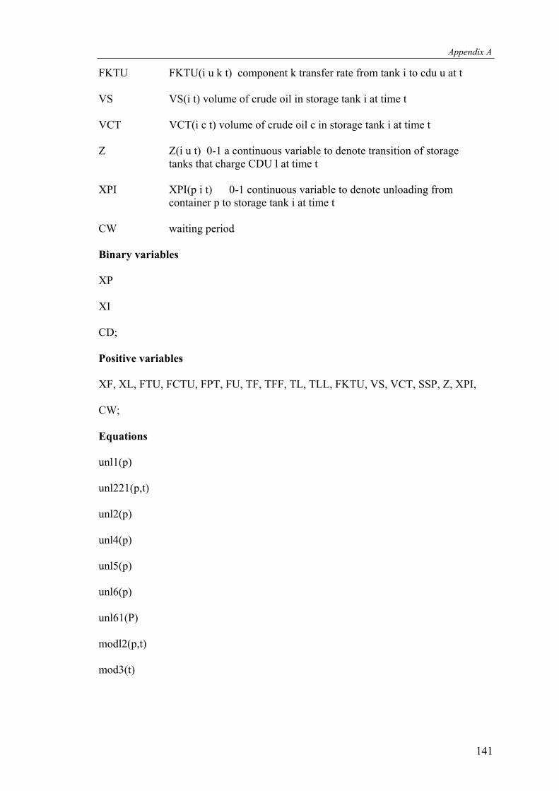
Appendix A
FKTU FKTU(i u k t) component k transfer rate from tank i to cdu u at t VS VS(i t) volume of crude oil in storage tank i at time t VCT VCT(i c t) volume of crude oil c in storage tank i at time t Z Z(i u t) 0-1 a continuous variable to denote transition of storage tanks that charge CDU l at time t XPI XPI(p i t) 0-1 continuous variable to denote unloading from container p to storage tank i at time t CW waiting period Binary variables XP XI CD; Positive variables XF, XL, FTU, FCTU, FPT, FU, TF, TFF, TL, TLL, FKTU, VS, VCT, SSP, Z, XPI, CW; Equations unl1(p) unl221(p,t) unl2(p) unl4(p) unl5(p) unl6(p) unl61(P) modl2(p,t) mod3(t)
141
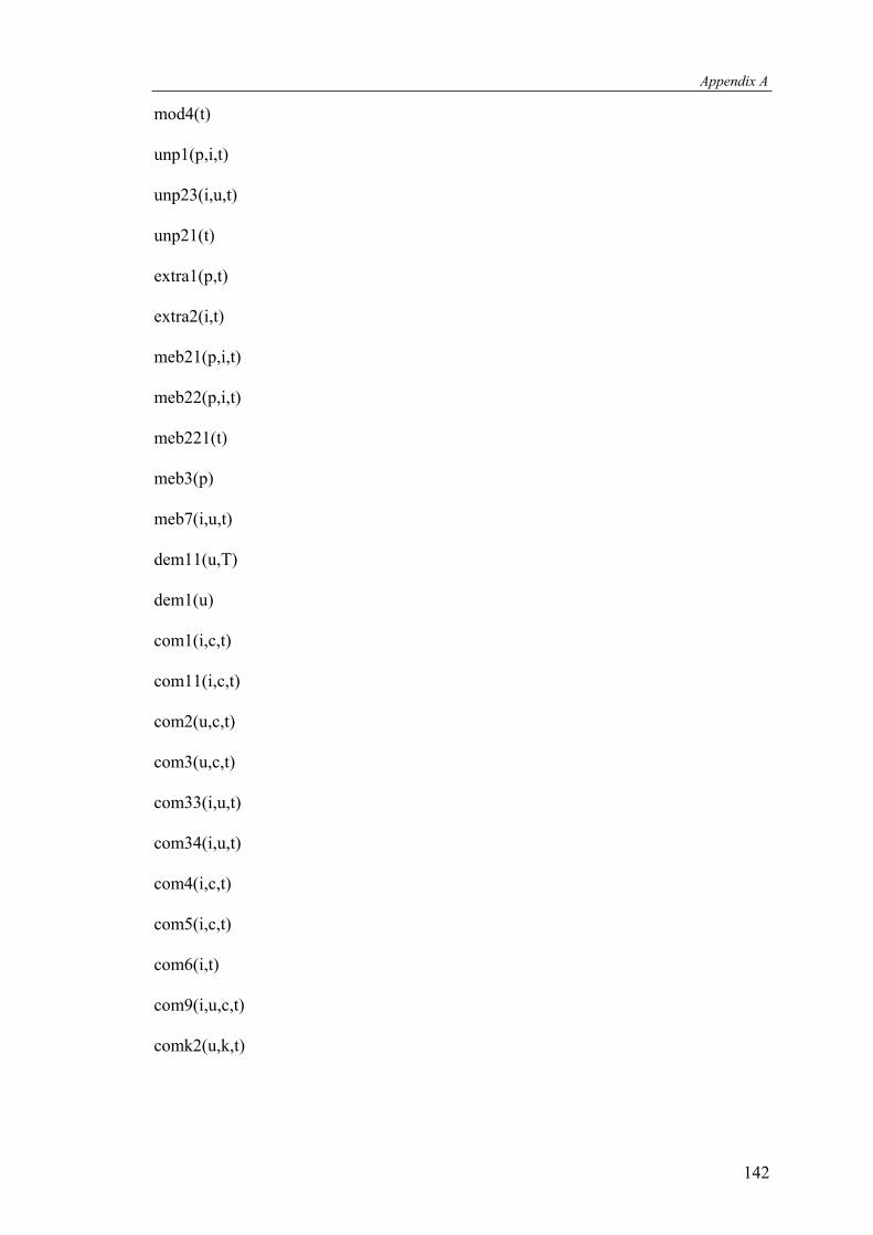
Appendix A
mod4(t) unp1(p,i,t) unp23(i,u,t) unp21(t) extra1(p,t) extra2(i,t) meb21(p,i,t) meb22(p,i,t) meb221(t) meb3(p) meb7(i,u,t) dem11(u,T) dem1(u) com1(i,c,t) com11(i,c,t) com2(u,c,t) com3(u,c,t) com33(i,u,t) com34(i,u,t) com4(i,c,t) com5(i,c,t) com6(i,t) com9(i,u,c,t) comk2(u,k,t)
142

Appendix A
comk3(u,k,t) char1(i,t) char2(u,t) chg21(i,u,T) chg22(i,u,T) extra4(t) extra5(v,p) OBJ2 ; *Constraints unl1(p)..sum(t$PT(p,t),XF(p,t))=e=1; unl221(p,t)$PT(p,t)..XP(p,t)=e=XP(p,t-1)+XF(p,t)-XL(p,t-1); unl2(p)..sum(t$PT(p,t),XL(p,t))=e=1; unl4(p)..TFF(p)=e=sum(t$PT(p,t),(ord(t))*XF(p,t))-1; unl5(p)..TLL(p)=e=sum(t$PT(p,t),ord(t)*XL(p,t)); unl6(p)$(ord(p) lt card(p))..TFF(p+1)=g=TLL(p)-1; unl61(P)..TLL(p)=g=TFF(p)+1; modl2(p,t)$PT(p,t)..XP(p,t)=g=XL(p,t); mod3(t)..sum(p$PT(p,t),XP(p,t))=l=2; mod4(t)..sum(i,XI(i,t))=l=2; extra1(p,t)$PT(p,t)..sum(i$PIT(p,i,t),XPI(p,i,t))=l=2*XP(p,t); extra2(i,t)..sum(p$PIT(p,i,t),XPI(p,i,t))=l=2*XI(i,t); unp1(p,i,t)$PIT(p,i,t)..XPI(p,i,t)=g=XP(p,t)+XI(i,t)-1; unp21(t)..sum((p,i)$PIT(p,i,t),XPI(p,i,t))=l=2; unp23(i,u,t)$IU(I,u)..2*XI(i,t)+CD(i,u,t)+CD(i,u,t+1)=l=2;
143

Appendix A
meb21(p,i,t)$(PIT(p,i,t))..FPTMIN*XPI(p,i,t)=l=FPT(p,i,t); meb22(p,i,t)$(PIT(p,i,t))..FPT(p,i,t)=l=FPTMAX*XPI(p,i,t); meb221(t)..sum((p,i)$PIT(p,i,t),FPT(p,i,t))/FPTMAX =l=1; meb3(p)..sum((i,t)$(PIT(p,i,t)),FPT(p,i,t))=e=VV0(p); meb7(i,u,t)$(IU(i,u))..FTU(i,u,t)=e=sum(c$(IC(i,c)and
UC(u,c)),FCTU(i,u,c,t));
dem11(u,t)..FU(u,t)=e=sum(i$IU(i,u),FTU(i,u,t)); dem1(u)..sum(t,FU(u,t))=e=DM(u); com1(i,c,t)$(IC(i,c) and (ord(t) gt 1))..VCT(i,c,t)=E=VCT(i,c,t-1)+SUM(p$(PC(p,c)
and PIT(p,i,t)),FPT(p,i,t)*EV(p,c))-SUM(u$IU(i,u),FCTU(i,u,c,t));
com11(i,c,t)$(IC(i,c) and (ord(t) eq 1))..VCT(i,c,t)=e=VSC0(i,c)+SUM(p$(PC(p,c) and PIT(p,i,t)),FPT(p,i,t)*EV(p,c))-SUM(u$IU(i,u),FCTU(i,u,c,t));
com2(u,c,t)..FU(u,t)*ESCMIN(c,u)=l=sum(i$(IU(i,u) and IC(i,c)),FCTU(i,u,c,t)); com3(u,c,t)..sum(i$(IU(i,u) and IC(i,c)),FCTU(i,u,c,t))=l=FU(u,t)*ESCMAX(c,u); com33(i,u,t)$(IU(i,u))..FTU(i,u,t)=L=FTUMAX*CD(i,u,t); com34(i,u,t)$(IU(i,u))..FTUMIN*CD(i,u,t)=L=FTU(i,u,t); com4(i,c,t)$(IC(i,c))..VS(i,t)*ESMIN(i,c)=l=VCT(i,c,t); com5(i,c,t)$(IC(i,c))..VCT(i,c,t)=l=VS(i,t)*ESMAX(i,c); com6(i,t)..sum(c$IC(i,c), VCT(i,c,t))=e=VS(i,t); com9(i,u,c,t)$(IU(i,u) and IC(i,c)and
FI(i,t))..FCTU(i,u,c,t)*VS0(i)=e=VSC0(i,c)*FTU(i,u,t);
comk2(u,k,t)..ELMIN(u,k)*sum(i$IU(i,u),FTU(i,u,t))=l=sum((i,c)$(IU(i,u) and IC(i,c) and UC(u,c)),FCTU(i,u,c,t)*EC(c,k));
comk3(u,k,t)..sum((i,c)$(IU(i,u) and IC(i,c) andUC(u,c)),FCTU(i,u,c,t)*EC(c,k))
=l=ELMAX(u,k)*SUM(i$IU(i,u),FTU(i,u,t));
char1(i,t)..sum(u$IU(i,u),CD(i,u,t))=l=2; char2(u,t)..sum(i$IU(i,u),CD(i,u,t))=l=2;
144
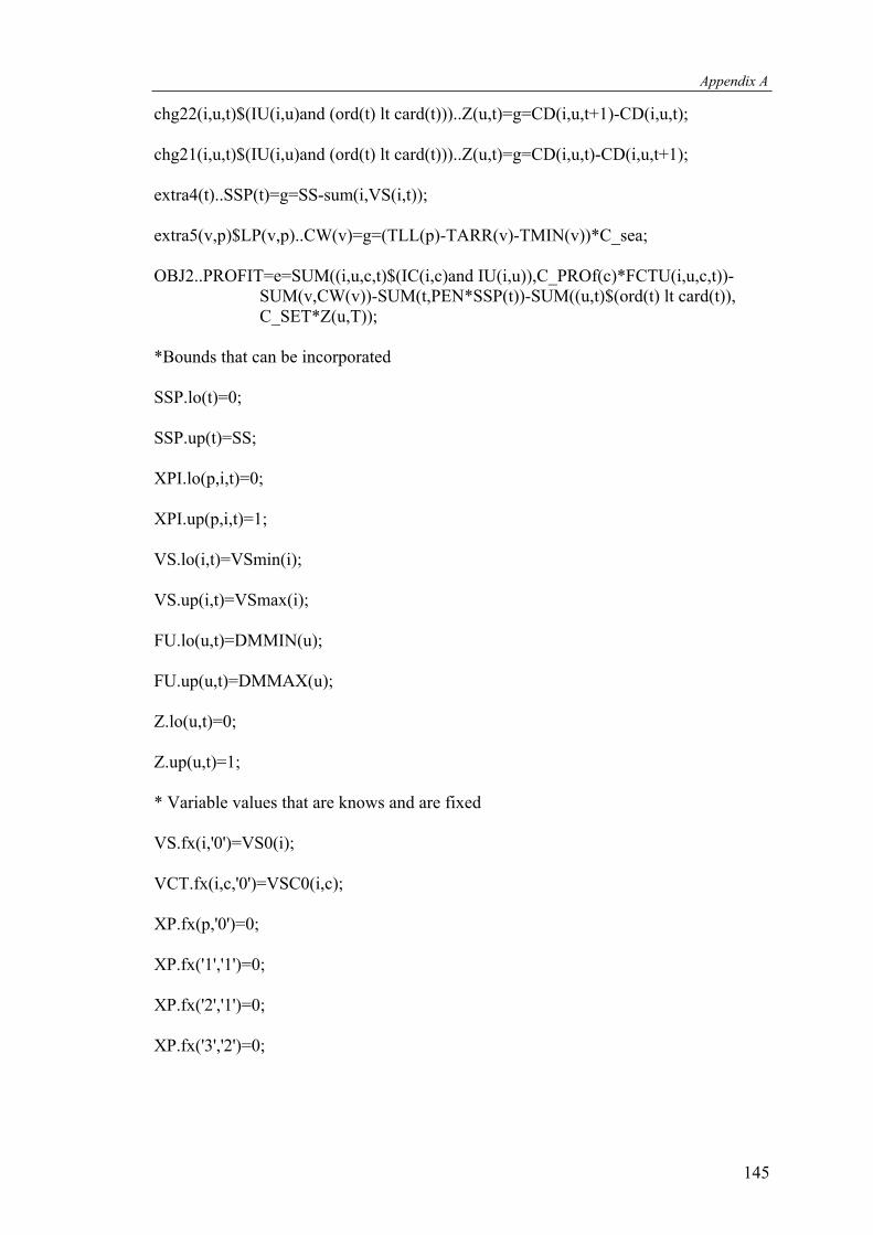
Appendix A
chg22(i,u,t)$(IU(i,u)and (ord(t) lt card(t)))..Z(u,t)=g=CD(i,u,t+1)-CD(i,u,t); chg21(i,u,t)$(IU(i,u)and (ord(t) lt card(t)))..Z(u,t)=g=CD(i,u,t)-CD(i,u,t+1); extra4(t)..SSP(t)=g=SS-sum(i,VS(i,t)); extra5(v,p)$LP(v,p)..CW(v)=g=(TLL(p)-TARR(v)-TMIN(v))*C_sea; OBJ2..PROFIT=e=SUM((i,u,c,t)$(IC(i,c)and IU(i,u)),C_PROf(c)*FCTU(i,u,c,t))-
SUM(v,CW(v))-SUM(t,PEN*SSP(t))-SUM((u,t)$(ord(t) lt card(t)), C_SET*Z(u,T));
*Bounds that can be incorporated SSP.lo(t)=0; SSP.up(t)=SS; XPI.lo(p,i,t)=0; XPI.up(p,i,t)=1; VS.lo(i,t)=VSmin(i); VS.up(i,t)=VSmax(i); FU.lo(u,t)=DMMIN(u); FU.up(u,t)=DMMAX(u); Z.lo(u,t)=0; Z.up(u,t)=1; * Variable values that are knows and are fixed VS.fx(i,'0')=VS0(i); VCT.fx(i,c,'0')=VSC0(i,c); XP.fx(p,'0')=0; XP.fx('1','1')=0; XP.fx('2','1')=0; XP.fx('3','2')=0;
145

Appendix A
XP.fx('4','2')=0; XI.fx(i,'6')=0; XI.fx(i,'7')=0; XI.fx(i,'8')=0; XI.fx(i,'9')=0; XI.fx(i,'10')=0; XI.fx(i,'1')=0; XI.fx('1','4')=0; XI.fx('6','4')=0; XI.fx('7','4')=0; XI.fx('1','5')=0; XI.fx('6','5')=0; XI.fx('7','5')=0; XI.fx('8','5')=0; XI.fx('2','2')=0; XI.fx('3','2')=0; XI.fx('4','2')=0; XI.fx('5','2')=0; * Model definition Model ResearchProblem /all/; ResearchProblem.optca=0.01; ResearchProblem.optcr=0.00; ResearchProblem.iterlim = 10000000; ResearchProblem.reslim = 1000000;
146

Appendix A
Solve ResearchProblem maximizing profit using MIP; Parameter f(i,c,t) r NE NE1 NET NET1 Next Next1 ; NE=0; NE1=0; NET=0; NET1=0; Next=0; Next1=0; r=3; Equation compiter(i,u,c,t) compiter2(i,u,c,t) compiter3(i,u,c,t) ; compiter(i,u,c,t)$(IU(i,u) and IC(i,c) and (ord(t)le r)) .. FCTU(i,u,c,t) =e=
f(i,c,t)*FTU(i,u,t);
compiter2(i,u,c,t)$(IU(i,u) and RCC(i,c) and (ord(t)ge NE) and (ord(t)le NE1)).. FCTU(i,u,c,t)=e=f(i,c,t)*FTU(i,u,t);
147
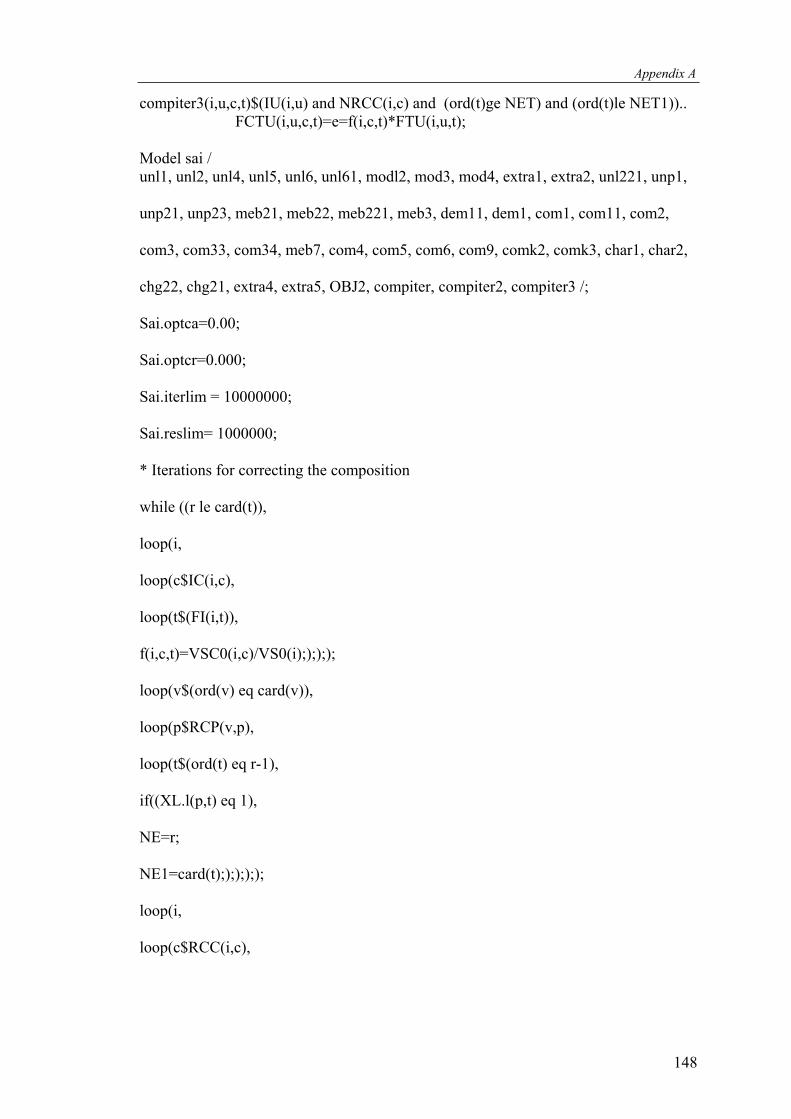
Appendix A
compiter3(i,u,c,t)$(IU(i,u) and NRCC(i,c) and (ord(t)ge NET) and (ord(t)le NET1)).. FCTU(i,u,c,t)=e=f(i,c,t)*FTU(i,u,t);
Model sai / unl1, unl2, unl4, unl5, unl6, unl61, modl2, mod3, mod4, extra1, extra2, unl221, unp1, unp21, unp23, meb21, meb22, meb221, meb3, dem11, dem1, com1, com11, com2, com3, com33, com34, meb7, com4, com5, com6, com9, comk2, comk3, char1, char2, chg22, chg21, extra4, extra5, OBJ2, compiter, compiter2, compiter3 /; Sai.optca=0.00; Sai.optcr=0.000; Sai.iterlim = 10000000; Sai.reslim= 1000000; * Iterations for correcting the composition while ((r le card(t)), loop(i, loop(c$IC(i,c), loop(t$(FI(i,t)), f(i,c,t)=VSC0(i,c)/VS0(i);););); loop(v$(ord(v) eq card(v)), loop(p$RCP(v,p), loop(t$(ord(t) eq r-1), if((XL.l(p,t) eq 1), NE=r; NE1=card(t););););); loop(i, loop(c$RCC(i,c),
148
Appendix A
loop(tt$(ord(tt) eq NE), loop(t$((ord(t) ge NE) and (ord(t) le NE1)), f(i,c,t)=VCT.l(i,c,tt-1)/VS.l(i,tt-1); );););); loop(v$(ord(v) eq card(v)), loop(p$NRP(v,p), loop(t$(ord(t) eq r-1), if((XL.l(p,t) eq 1), NET=r; NET1=card(t););););); loop(i, loop(c$NRCC(i,c), loop(tt$(ord(tt) eq Net), loop(t$((ord(t) ge NET) and (ord(t) le NET1)), f(i,c,t)=vct.l(i,c,tt-1)/vs.l(i,tt-1););););); loop(i, loop(c$IC(i,c), loop(t$((ord(t)le r)and (ord(t) gt 1)), f(i,c,t)=VCT.l(i,c,t-1)/VS.l(i,t-1);););); loop(v$(ord(v) eq card(v)), loop(p$LP(v,p), loop(t$(ord(t)eq r-1), if((xl.l(p,t) eq 1), Next=r; Next1=card(t);););););
149

Appendix A
loop(u, loop(i$(IU(i,u)), loop(c$IC(i,c), loop(t$(ord(t)le r-1), FTU.fx(i,u,t)=FTU.l(i,u,t); CD.fx(i,u,t)=CD.l(i,u,t); VS.fx(i,t)=VS.l(i,t); FCTU.fx(i,u,c,t)=FCTU.l(i,u,c,t); VCT.fx(i,c,t)=VCT.l(i,c,t); );););) loop(p, loop(i$PI(p,i), loop(t$(ord(t)le r-1), XPI.fx(p,i,t)=XPI.l(p,i,t); XP.fx(p,t)=XP.l(p,t); XI.fx(i,t)=XI.l(i,t); XL.fx(p,t)=XL.l(p,t); XF.fx(p,t)=XF.l(p,t); FPT.fx(p,i,t)=FPT.l(p,i,t);););); * Adjusting the optimality gap as the problem size decreases if(r gt 2, Sai.optcr=0.0;); Solve Sai maximizing profit using MIP; Display XF.l, XL.l, TFF.l, TLL.l, XP.l, XI.l, XPI.L, CD.l, Z.l, FPT.l, FTU.l, FCTU.l,
VS.l, VCT.l, PROFIT.L, NE, NE1, NET, NET1; * Incase if r is reached a criteria to end of horizon then assign it as end else increment
150
Appendix A
if((r eq Next), r=Next1 ;); r=r+1; ); Display XF.L, XL.L, XP.l, XI.l, XPI.L, CD.l, Z.l, FPT.l, FTU.l, FCTU.l, VS.l, VCT.l,
PROFIT.L, NE, NE1, NET, NET1;
151
Appendix A
A.2: GAMS file – continuous time model for example-1 of part II
$TITLE Example 1 of Part2 continuous time modeling approach
OPTION solprint =off;
OPTION MIP =cplex;
OPTION limrow = 0;
OPTION limcol = 0;
OPTION sysout =off;
* Set definitions.
Sets
C different types of crudes /1*8/
I crude oil storage tank /1*8/
K key component of crude oil /1/
U crude distillation units /1*3/
T time interval /1*3/
V crude vessel /1/
P compartments /1*4/
S slots /1*7/
RCC(i,c) RCC crude types /1.(1*4), (6*8).(1*4)/
NRCC(i,c) NRCC crude types /(2*5).(5*8)/
CST(t,s) combination of slots and time periods /1.(1), 2.(2*6), 3.(7)/
CPS(p,s) combination of slots and parcels in which the parcel can be
possibly get unloaded /1.(2), 2.(3*4),3.(4*5), 4.(5*6)/ VP(v,p) oil types that vessel carries /1.(1*4)/
152
Appendix A
FP(v,p) set of first containers of crude vessel v /1.1/ LP(v,p) set of last containers of crude vessel v /1.4/ RCP(v,p) last RCC parcel and vessel combination /1.3/ NRP(v,p) last NRCC parcel and vessel combination /1.4/ RP(v,p) RCC parcels and vessel combinations /1.(1*3)/ NP(v,p) NRCC parcels and vessel combinations /1.(4)/ RFP(v,p) First RCC parcel and vessel combinations /1.1/ NFP(v,p) First NRCC parcels and vessel combinations /1.4/ IC(i,c) oil types in storage tanks /1.1*4, 2.5*8, 3.5*8, 4.5*8, 5.5*8, 6.1*4, 7.1*4, 8.1*4/ IU(i,u) probable Storage tanks that can be given to CDUs /1.3, 2.1*2, 3.1*2, 4.1*2, 5.(1*2), 6.3, 7.3, 8.3/ UC(u,c) crudes that CDU u can process /1.(5*8), 2.(5*8), 3.(1*4)/ PC(p,c) crudes that are being carried by containers /1.2, 2.3, 3.4, 4.5/ PI(p,i) feasible storage tank i for vessel v /1.(1),1.(6*8), 2.(1), 2.(6*8), 3.1, 3.(6*8), 4.(2*5)/ Last(t,s) last slot in period t /1.1, 2.6, 3.7/ VLP(p) vessel last parcel /4/ FI(i,s) constant composition slots /1.(1*2), (2*5).(1*5), (6*8).(1*2)/ Alias(s,ss); Alias(s,sss); Alias(i,ii); Alias(p,pp); CSS(s,ss) slot combinations for settling time /2.(3*4), 3.(4*5), 4.(5*6), 5.(6*7)/ RP1(v,pp) RCC parcels and vessel combinations /1.(1*3)/
153

Appendix A
NP1(v,pp) NRCC parcels and vessel combinations /1.(4)/ RFP1(v,pp) First RCC parcel and vessel combinations /1.1/ NFP1(v,pp) First NRCC parcels and vessel combinations /1.4/ IU1(ii,u) Probable Storage tanks that can be given to CDUs /1.3, 2.1*2, 3.1*2, 4.1*2, 5.(1*2), 6.3, 7.3, 8.3/ IC1(ii,c) oil types in storage tanks /1.1*4, 2.5*8, 3.5*8, 4.5*8, 5.5*8, 6.1*4, 7.1*4, 8.1*4/ CST1(t,ss) combination of slots and time periods /1.(1), 2.(2*6), 3.(7)/ CST2(t,sss) combination of slots and time periods /1.(1), 2.(2*6), 3.(7)/ CPS2(pp,ss) combination of slots and parcels in which the parcel can be possibly get unloaded /1.(2), 2.(3*4),3.(4*5), 4.(5*6)/ Parameters C_prof(c) margin profits of crude c /1 1.5, 2 1.7, 3 1.5, 4 1.6, 5 1.45, 6 1.6, 7 1.55, 8 1.6/ C_SEA sea waiting cost of vessel v per unit time interval /3.125/ C_SET change over cost for crude mix transition toCDU u /5/ PEN(t) penalty for safety stock per period /1 0.375, 2 0.5, 3 0.925/ DM(u) demand of crude mix j by cdus during the schedule horizon /1 300, 2 300, 3 300/ DMMIN(u) minimum demand of crude oil by CDU u each hr /1 2, 2 2, 3 2/ DMMAX(u) maximum demand of crude oil by CDU u each hr /1 6, 2 6, 3 6/ EV(p,c) concentration of crude oil c in vessel v /1.2 1, 2.3 1, 3.4 1, 4.5 1/ EC(c,k) key component in crude /1.1 0.002, 2.1 0.0025, 3.1 0.0015, 4.1 0.006, 5.1 0.012, 6.1 0.013, 7.1 0.009, 8.1 0.015/ ELMIN(u,k) Limits on key components in CDU u feed /1.1 0.001, 2.1 0.001, 3.1 0.001/ ELMAX(u,K) /1.1 0.014, 2.1 0.0130, 3.1 0.004/
154
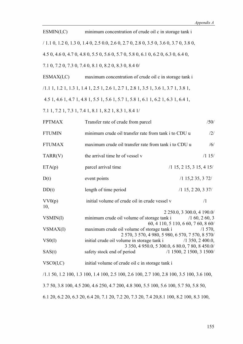
Appendix A
ESMIN(I,C) minimum concentration of crude oil c in storage tank i / 1.1 0, 1.2 0, 1.3 0, 1.4 0, 2.5 0.0, 2.6 0, 2.7 0, 2.8 0, 3.5 0, 3.6 0, 3.7 0, 3.8 0, 4.5 0, 4.6 0, 4.7 0, 4.8 0, 5.5 0, 5.6 0, 5.7 0, 5.8 0, 6.1 0, 6.2 0, 6.3 0, 6.4 0, 7.1 0, 7.2 0, 7.3 0, 7.4 0, 8.1 0, 8.2 0, 8.3 0, 8.4 0/ ESMAX(I,C) maximum concentration of crude oil c in storage tank i /1.1 1, 1.2 1, 1.3 1, 1.4 1, 2.5 1, 2.6 1, 2.7 1, 2.8 1, 3.5 1, 3.6 1, 3.7 1, 3.8 1, 4.5 1, 4.6 1, 4.7 1, 4.8 1, 5.5 1, 5.6 1, 5.7 1, 5.8 1, 6.1 1, 6.2 1, 6.3 1, 6.4 1, 7.1 1, 7.2 1, 7.3 1, 7.4 1, 8.1 1, 8.2 1, 8.3 1, 8.4 1/ FPTMAX Transfer rate of crude from parcel /50/ FTUMIN minimum crude oil transfer rate from tank i to CDU u /2/ FTUMAX maximum crude oil transfer rate from tank i to CDU u /6/ TARR(V) the arrival time hr of vessel v /1 15/ ETA(p) parcel arrival time /1 15, 2 15, 3 15, 4 15/ D(t) event points /1 15,2 35, 3 72/ DD(t) length of time period /1 15, 2 20, 3 37/ VV0(p) initial volume of crude oil in crude vessel v /1 10, 2 250.0, 3 300.0, 4 190.0/ VSMIN(I) minimum crude oil volume of storage tank i /1 60, 2 60, 3 60, 4 110, 5 110, 6 60, 7 60, 8 60/ VSMAX(I) maximum crude oil volume of storage tank i /1 570, 2 570, 3 570, 4 980, 5 980, 6 570, 7 570, 8 570/ VS0(I) initial crude oil volume in storage tank i /1 350, 2 400.0, 3 350, 4 950.0, 5 300.0, 6 80.0, 7 80, 8 450.0/ SAS(t) safety stock end of period /1 1500, 2 1500, 3 1500/ VSC0(I,C) initial volume of crude oil c in storage tank i /1.1 50, 1.2 100, 1.3 100, 1.4 100, 2.5 100, 2.6 100, 2.7 100, 2.8 100, 3.5 100, 3.6 100, 3.7 50, 3.8 100, 4.5 200, 4.6 250, 4.7 200, 4.8 300, 5.5 100, 5.6 100, 5.7 50, 5.8 50, 6.1 20, 6.2 20, 6.3 20, 6.4 20, 7.1 20, 7.2 20, 7.3 20, 7.4 20,8.1 100, 8.2 100, 8.3 100,
155
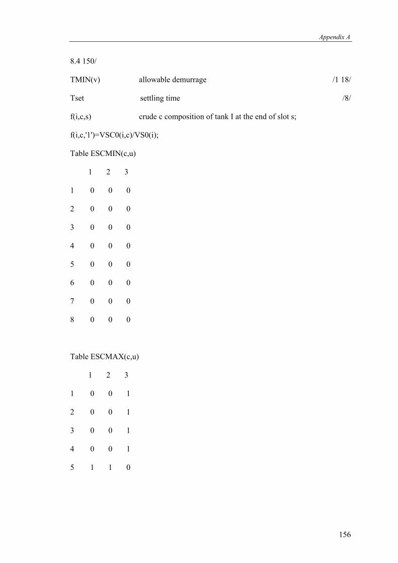
Appendix A
8.4 150/ TMIN(v) allowable demurrage /1 18/ Tset settling time /8/ f(i,c,s) crude c composition of tank I at the end of slot s; f(i,c,'1')=VSC0(i,c)/VS0(i); Table ESCMIN(c,u) 1 2 3 1 0 0 0 2 0 0 0 3 0 0 0 4 0 0 0 5 0 0 0 6 0 0 0 7 0 0 0 8 0 0 0 Table ESCMAX(c,u) 1 2 3 1 0 0 1 2 0 0 1 3 0 0 1 4 0 0 1 5 1 1 0
156
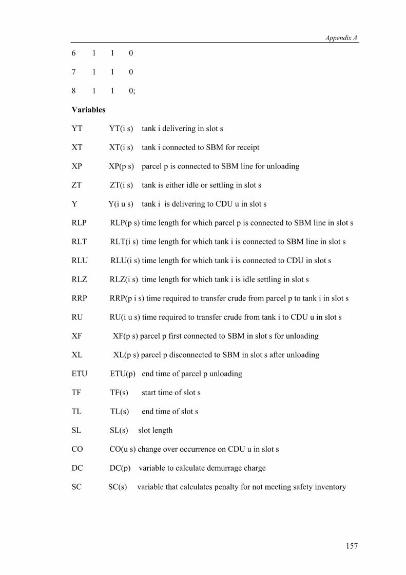
Appendix A
6 1 1 0 7 1 1 0 8 1 1 0; Variables YT YT(i s) tank i delivering in slot s XT XT(i s) tank i connected to SBM for receipt XP XP(p s) parcel p is connected to SBM line for unloading ZT ZT(i s) tank is either idle or settling in slot s Y Y(i u s) tank i is delivering to CDU u in slot s RLP RLP(p s) time length for which parcel p is connected to SBM line in slot s RLT RLT(i s) time length for which tank i is connected to SBM line in slot s RLU RLU(i s) time length for which tank i is connected to CDU in slot s RLZ RLZ(i s) time length for which tank i is idle settling in slot s RRP RRP(p i s) time required to transfer crude from parcel p to tank i in slot s RU RU(i u s) time required to transfer crude from tank i to CDU u in slot s XF XF(p s) parcel p first connected to SBM in slot s for unloading XL XL(p s) parcel p disconnected to SBM in slot s after unloading ETU ETU(p) end time of parcel p unloading TF TF(s) start time of slot s TL TL(s) end time of slot s SL SL(s) slot length CO CO(u s) change over occurrence on CDU u in slot s DC DC(p) variable to calculate demurrage charge SC SC(s) variable that calculates penalty for not meeting safety inventory
157
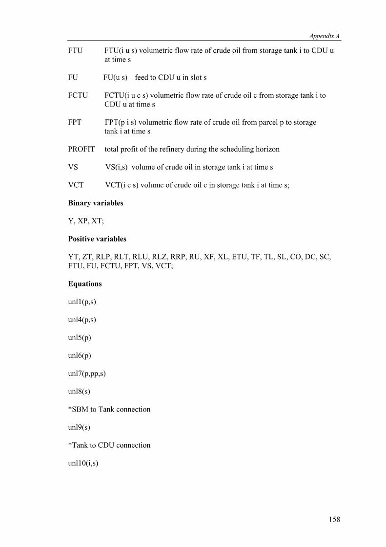
Appendix A
FTU FTU(i u s) volumetric flow rate of crude oil from storage tank i to CDU u at time s FU FU(u s) feed to CDU u in slot s FCTU FCTU(i u c s) volumetric flow rate of crude oil c from storage tank i to CDU u at time s FPT FPT(p i s) volumetric flow rate of crude oil from parcel p to storage tank i at time s PROFIT total profit of the refinery during the scheduling horizon VS VS(i,s) volume of crude oil in storage tank i at time s VCT VCT(i c s) volume of crude oil c in storage tank i at time s; Binary variables Y, XP, XT; Positive variables YT, ZT, RLP, RLT, RLU, RLZ, RRP, RU, XF, XL, ETU, TF, TL, SL, CO, DC, SC, FTU, FU, FCTU, FPT, VS, VCT; Equations unl1(p,s) unl4(p,s) unl5(p) unl6(p) unl7(p,pp,s) unl8(s) *SBM to Tank connection unl9(s) *Tank to CDU connection unl10(i,s)
158
Appendix A
unl11(u,s) *Activity assignment act1(i,u,s) act2(i,s) act3(i,s) *Activity time accounting act4(s) act5(s) act6(p,s,t) act7(s) act8(i,s,t) act9(s) act10(s) act11(i,s,t) act12(i,s,t) act13(i,s) * Crude transfer from parcel to tank ulp3(p,i,s) ulp4(i,s) ulp5(p,s) ulp6(t) ulp7(p,i,s) ulp8(p) *Crude transfer from tank to CDUs
159

Appendix A
chr1(i,u,s,t) chr2(i,u,s,t) chr3(i,u,s) chr4(i,u,s) chr5(i,u,s) chr6(i,u,s) chr7(u,s) chr8(u,s) chr9(u,s) chr10(u) chr11(i,u,c,s) *Crude balance bal1(i,c,s) bal2(i,c,s) bal3(i,s) *Component balance com1(u,c,s) com12(u,c,s) com2(i,c,s) com22(i,c,s) com3(u,k,s) com32(u,k,s) *Change over calculation co1(i,u,s)
160

Appendix A
co2(i,u,s) *Settling time set1(i,s) set2(i,s,ss) *Demurrage accounting,safety inventory penalty accounting extra4(t,s) extra5(v,p,s,t) * Objective function OBJ2 ; *equations *parcel to SBM connections unl1(p,s)$CPS(p,s)..XP(p,s+1)=e=XP(p,s)+XF(p,s+1)-XL(p,s); unl4(p,s)$CPS(p,s)..XL(p,s)=l=XP(p,s); unl5(p)..sum(s$CPS(p,s),XF(p,s))=e=1; unl6(p)..sum(s$CPS(p,s),XL(p,s))=e=1; unl7(p,pp,s)$(CPS(p,s)and (ord(pp) eq (ord(p)-1)))..XF(p,s)=l=sum(ss$((ord(ss) lt ord(s)) and CPS2(pp,ss)),XL(pp,ss)); unl8(s)..sum(p$CPS(p,s), XP(p,s))=l=1; *SBM to Tank connection unl9(s)..sum(i,XT(i,s))=l=sum(p$CPS(p,s),XP(p,s)); *Tank to CDU connection unl10(i,s)..sum(u$IU(i,u),Y(i,u,s))=l=2; unl11(u,s)..sum(i$IU(i,u),Y(i,u,s))=l=2; *Activity assignment
161

Appendix A
act1(i,u,s)$IU(i,u)..YT(i,s)=g=Y(i,u,s); act2(i,s)..sum(u$IU(i,u),Y(i,u,s))=g=YT(i,s); act3(i,s)..XT(i,s)+YT(i,s)+ZT(i,s)=e=1; *Activity time accounting act4(s)$(ord(s) gt 1)..TL(s)=e=TL(s-1)+SL(s); act5(s)$(ord(s) eq 1)..TL(s)=e=TL('0')+SL(s); act6(p,s,t)$(CST(t,s)and CPS(p,s))..RLP(p,s)=l=DD(t)*XP(p,s); act7(s)..sum(p$CPS(p,s),RLP(p,s))=l=SL(s); act8(i,s,t)$CST(t,s)..RLT(i,s)=l=DD(t)*XT(i,s); act9(s)..sum(i,RLT(i,s))=l=SL(s); act10(s)..sum(i,RLT(i,s))=l=sum(p$CPS(p,s),RLP(p,s)); act11(i,s,t)$CST(t,s)..RLU(i,s)=l=DD(t)*YT(i,s); act12(i,s,t)$CST(t,s)..RLZ(i,s)=l=DD(t)*ZT(i,s); act13(i,s)..RLT(i,s)+RLU(i,s)+RLZ(i,s)=e=SL(s); * Crude transfer from parcel to tank ulp3(p,i,s)$(PI(p,i) and CPS(p,s))..RRP(p,i,s)=g=RLT(i,s)+RLP(p,s)-SL(s); ulp4(i,s)..sum(p$(PI(p,i)and CPS(p,s)),RRP(p,i,s))=l=RLT(i,s); ulp5(p,s)$(CPS(p,s))..sum(i$PI(p,i),RRP(p,i,s))=l=RLP(p,s); ulp6(t)..sum(s$cst(t,s),SL(s))=e=DD(t); ulp7(p,i,s)$(PI(p,i) and CPS(p,s))..FPT(p,i,s)=e=FPTmax*RRP(p,i,s); ulp8(p)..sum((i,s)$(PI(p,i) and CPS(p,s)),FPT(p,i,s))=e=VV0(p); *Crude transfer from tank to CDUs chr1(i,u,s,t)$(IU(i,u) and CST(t,s))..RU(i,u,s)=l=DD(t)*Y(i,u,s); chr 2(i,u,s,t)$(IU(i,u) and CST(t,s))..RU(i,u,s)=g=RLU(i,s)-DD(t)*(1-Y(i,u,s));
162

Appendix A
chr 3(i,u,s)$IU(i,u)..RU(i,u,s)=l=RLU(i,s); chr 4(i,u,s)$IU(i,u)..FTUmin*RU(i,u,s)=l=FTU(i,u,s); chr 5(i,u,s)$IU(i,u)..FTUmax*RU(i,u,s)=g=FTU(i,u,s); chr 6(i,u,s)$IU(i,u)..FTU(i,u,s)=e=sum(c$IC(i,c),FCTU(i,u,c,s)); chr 7(u,s)..FU(u,s)=e=sum(i$IU(i,u),FTU(i,u,s)); chr 8(u,s)..DMmin(u)*SL(s)=l=FU(u,s); chr 9(u,s)..FU(u,s)=l=DMmax(u)*SL(s); chr 10(u)..sum(s,FU(u,s))=e=DM(u); chr 11(i,u,c,s)$(IU(i,u) and IC(i,c)and FI(i,s))..FCTU(i,u,c,s)=e=f(i,c,'1')*FTU(i,u,s); *Crude balance bal1(i,c,s)$(IC(i,c)and (ord(s) gt 1))..VCT(i,c,s)=e=VCT(i,c,s-1)+sum(p$(PI(p,i) and PC(p,c)and CPS(p,s)),FPT(p,i,s))-Sum(u$IU(i,u),FCTU(i,u,c,s)); bal 2(i,c,s)$(IC(i,c)and (ord(s) eq 1))..VCT(i,c,s)=e=VSC0(i,c)+sum(p$(PI(p,i) and PC(p,c)and CPS(p,s)),FPT(p,i,s))-Sum(u$IU(i,u),FCTU(i,u,c,s)); bal 3(i,s)..VS(i,s)=e=Sum(c$IC(i,c),VCT(i,c,s)); *component balance com1(u,c,s)..FU(u,s)*ESCmin(c,u)=l=sum(i$(IC(i,c) and IU(i,u)),FCTU(i,u,c,s)); com 12(u,c,s)..sum(i$(IC(i,c) and IU(i,u)),FCTU(i,u,c,s))=l=FU(u,s)*ESCmax(c,u); com 2(i,c,s)$(IC(i,c))..VS(i,s)*ESmin(i,c)=l=VCT(i,c,s); com 22(i,c,s)$(IC(i,c))..VCT(i,c,s)=l=VS(i,s)*ESmax(i,c); com 3(u,k,s)..FU(u,s)*ELmin(u,k)=l=sum((i,c)$(IC(i,c) and IU(i,u)),FCTU(i,u,c,s)*EC(c,k)); com 32(u,k,s)..sum((i,c)$(IC(i,c) and IU(i,u)),FCTU(i,u,c,s)*EC(c,k))=l=FU(u,s)*ELmax(u,k); *change over calculation co1(i,u,s)$(IU(i,u)and (ord(s) lt card(s)))..CO(u,s)=g=Y(i,u,s)-Y(i,u,s+1);
163
Appendix A
co2(i,u,s)$(IU(i,u)and (ord(s) lt card(s)))..CO(u,s)=g=Y(i,u,s+1)-Y(i,u,s); *settling time set1(i,s)..XT(i,s)+YT(i,s+1)=l=1; set2(i,s,ss)$CSS(s,ss)..Tset*(YT(i,ss)+XT(i,s)-1)=l=TL(ss-1)-TL(s); *Demurrage accounting,safety inventory penalty accounting extra4(t,s)$(last(t,s))..SC(t)=g=pen(t)*(sAs(t)-sum(i,VS(i,s))); extra5(v,p,s,t)$(LP(v,p)and cps(p,s)and cst(t,s)) ..DC(v)=g=(TL(s)- (ETA(p)+Tmin(v))*XP(p,s)-D(t)*(1-XP(p,s)))*C_sea; * Objective function OBJ2..profit=e=sum((i,u,c,s)$(IU(i,u) and IC(i,c)),FCTU(i,u,c,s)*C_prof(c))- sum(v,DC(v))-C_set*sum((u,s),CO(u,s))-Sum(t,SC(t)); *Bounds that CAN BE INCORPORATED CO.lo(u,s)=0; CO.up(u,s)=1; YT.lo(i,s)=0; YT.up(i,s)=1; ZT.lo(i,s)=0; ZT.up(i,s)=1; VS.lo(i,s)=VSmin(i); VS.up(i,s)=VSmax(i); XF.lo(p,s)=0; XF.up(p,s)=1; XL.lo(p,s)=0; XL.up(p,s)=1; TL.fx('1')=D('1');
164

Appendix A
TL.fx('6')=D('2'); TL.fx('7')=D('3'); TL.fx('0')=0; VS.fx(i,'0')=VS0(i); VCT.fx(i,c,'0')=VSC0(i,c); XF.fx('1','1')=0; XL.fx('1','3')=0; XF.fx('2','2')=0; XL.fx('2','5')=0; XF.fx('3','3')=0; XL.fx('3','6')=0; XF.fx('4','4')=0; XL.fx('4','7')=0; XP.fx(p,'1')=0; XP.fx(p,'7')=0; XP.fx('1','3')=0; XP.fx('1','4')=0; XP.fx('1','5')=0; XP.fx('1','6')=0; XP.fx('2','2')=0; XP.fx('2','5')=0; XP.fx('2','6')=0; XP.fx('3','2')=0; XP.fx('3','3')=0;
165

Appendix A
XP.fx('3','6')=0; XP.fx('4','2')=0; XP.fx('4','3')=0; XP.fx('4','4')=0; XT.fx(i,'1')=0; XT.fx(i,'7')=0; XT.fx('1','6')=0; XT.fx('6','6')=0; XT.fx('7','6')=0; XT.fx('8','6')=0; XT.fx('2','2')=0; XT.fx('2','3')=0; XT.fx('2','4')=0; XT.fx('3','2')=0; XT.fx('3','3')=0; XT.fx('3','4')=0; XT.fx('4','2')=0; XT.fx('4','3')=0; XT.fx('4','4')=0; XT.fx('5','2')=0; XT.fx('5','3')=0; XT.fx('5','4')=0; Model ResearchProblem /all/; ResearchProblem.optca=0.00;
166
Appendix A
ResearchProblem.optcr=0.000; ResearchProblem.iterlim = 10000000; ResearchProblem.reslim= 1000000; Solve ResearchProblem maximizing profit using MIP; Display XF.l, XL.l, TL.L, SL.l, RLP.l, RLT.l, RLZ.l, RLU.l, RRP.l, RU.l, XP.l, XT.l, YT.l, ZT.l, Y.l, CO.l, FPT.l, FTU.l, FCTU.l, VS.l, VCT.l, PROFIT.L; Parameter f(i,c,s) r Next Next1 NE NE1 NET NET1; r=3; Next=0; Next1=0; NE=0; NE1=0; NET=0; NET1=0; Equation cor1(i,u,c,s)
167

Appendix A
cor5(i,u,c,s) cor6(i,u,c,s) cor7(i,u,c,s) ; cor1(i,u,c,s)$(IU(i,u) and IC(i,c) and (ord(s)le r))..FCTU(i,u,c,s)=e=f(i,c,s)*FTU(i,u,s); cor5(i,u,c,s)$(IU(i,u) and RCC(i,c) and (ord(s)ge NE) and (ord(s)le NE1))..FCTU(i,u,c,s)=e=f(i,c,s)*FTU(i,u,s); cor6(i,u,c,s)$(IU(i,u) and NRCC(i,c) and (ord(s)ge NET) and (ord(s)le NET1))..FCTU(i,u,c,s)=e=f(i,c,s)*FTU(i,u,s); cor7(i,u,c,s)$(IU(i,u) and IC(i,c) and (ord(s)ge Next) and (ord(s)le next1))..FCTU(i,u,c,s)=e=f(i,c,s)*FTU(i,u,s); Model Sai / unl1, unl4, unl5, unl6, unl7, unl8, unl9, unl10, unl11, act1, act2, act3, act4, act5, act6, act7, act8, act9, act10, act11, act12, act13, ulp3, ulp4, ulp5, ulp6, ulp7, ulp8, chr1, chr2, chr3, chr4, chr5, chr6, chr7, chr8, chr9, chr10, chr11, bal1, bal2, bal3, com1, com 12, com 2, com 22, com 3, com 32, co1, co2, set1, set2, extra4, extra5, cor1, cor5, cor6, cor7, OBJ2 /; Sai.optca=0.00; Sai.optcr=0.000; Sai.iterlim = 10000000; Sai.reslim= 1000000; While ((r le card(s)), loop(i, loop(c$IC(i,c), loop(s$((ord(s)le r)and (ord(s) gt 1)), f(i,c,s)=VCT.l(i,c,s-1)/VS.l(i,s-1);););); loop(v$(ord(v) eq card(v)),
168

Appendix A
loop(p$RCP(v,p), loop(s$(ord(s) eq r-1), if((XL.L(p,s) eq 1), NE=r; NE1=card(s););););); loop(i, loop(c$RCC(i,c), loop(ss$(ord(ss) eq NE), loop(s$((ord(s) ge NE) and (ord(s) le NE1)), f(i,c,s)=VCT.l(i,c,ss-1)/VS.l(i,ss-1););););); loop(v$(ord(v) eq card(v)), loop(p$NRP(v,p), loop(s$(ord(s) eq r-1), if((XL.L(p,s) eq 1), NET=r; NET1=card(s););););); loop(i, loop(c$NRCC(i,c), loop(ss$(ord(ss) eq NET), loop(s$((ord(s) ge NET) and (ord(s) le NET1)), f(i,c,s)=VCT.l(i,c,ss-1)/VS.l(i,ss-1););););); loop(v$(ord(v) eq card(v)), loop(p$LP(v,p), loop(s$(ord(s)eq r-1),
169
Appendix A
if((XLl.l(p,s) eq 1), Next=r; Next1=card(s););););); loop(u, loop(i$(IU(i,u)), loop(c$IC(i,c), loop(s$(ord(s)le r-1), FTU.fx(i,u,s)=FTU.l(i,u,s); Y.fx(i,u,s)=Y.l(i,u,s); VS.fx(i,s)=VS.l(i,s); FCTU.fx(i,u,c,s)=FCTU.l(i,u,c,s); VCT.fx(i,c,s)=VCT.l(i,c,s); SL.fx(s)=SL.l(s); RLU.fx(i,s)=RLU.l(i,s); RLT.fx(i,s)=RLT.l(i,s); RLZ.fx(i,s)=RLZ.l(i,s); YT.fx(i,s)=YT.l(i,s); ZT.fx(i,s)=ZT.l(i,s); XT.fx(i,s)=XT.l(i,s); RU.fx(i,u,s)=RU.l(i,u,s););););) loop(p, loop(i$PI(p,i), loop(s$(ord(s)le r-1), XP.fx(p,s)=XP.l(p,s);
170
Appendix A
171
XL.fx(p,s)=XL.l(p,s); XF.fx(p,s)=XF.l(p,s); FPT.fx(p,i,s)=FPT.l(p,i,s); RLP.fx(p,s)=RLP.l(p,s); RRP.fx(p,i,s)=RRP.l(p,i,s);););); Solve Sai maximizing profit using MIP; Display XF.l, XL.l, TL.L, SL.l, RLP.l, RLT.l, RLZ.l, RLU.l, RRP.l, RU.l, XP.l, XT.l, YT.l, ZT.l, Y.l, CO.l, FPT.l, FTU.l, FCTU.l, VS.l, VCT.l, PROFIT.L, Next, Next1, NE, NE1, NET, NET1; If((r eq Next), r=Next1;); r=r+1; Next=0; Next1=0;); Display XF.l, XL.l, TL.L, SL.l, RLP.l, RLT.l, RLZ.l, RLU.l, RRP.l, RU.l, XP.l, XT.l, YT.l, ZT.l, Y.l, CO.l, FPT.l, FTU.l, FCTU.l, VS.l, VCT.l, PROFIT.L, Next, Next1, NE, NE1, NET, NET1;