cs 4495 computer vision - georgia institute of technologyafb/classes/cs4495-fall2013/...cs 4495...
TRANSCRIPT
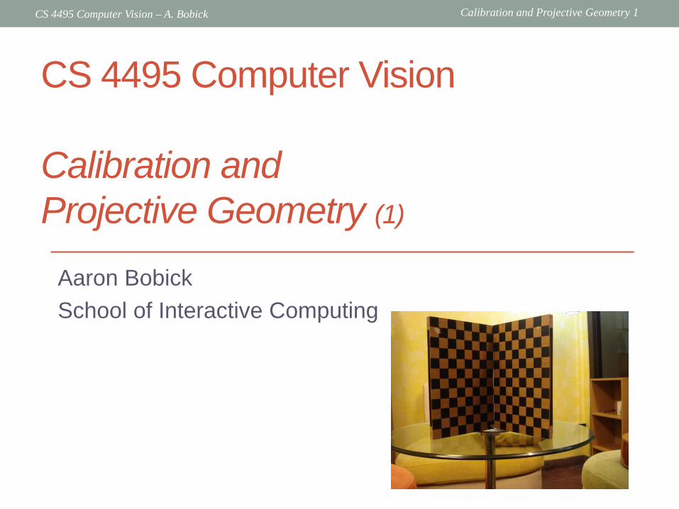
Calibration and Projective Geometry 1 CS 4495 Computer Vision – A. Bobick
Aaron Bobick School of Interactive Computing
CS 4495 Computer Vision Calibration and Projective Geometry (1)
Calibration and Projective Geometry 1 CS 4495 Computer Vision – A. Bobick
Administrivia • Problem set 2:
• What is the issue with finding the PDF???? http://www.cc.gatech.edu/~afb/classes/CS4495-Fall2013/
or http://www.cc.gatech.edu/~afb/classes/CS4495-Fall2013/ProblemSets/PS2/ps2-descr.pdf
• Today: Really using homogeneous systems to represent projection. And how to do calibration.
• Forsyth and Ponce, 1.2 and 1.3

Calibration and Projective Geometry 1 CS 4495 Computer Vision – A. Bobick
Last time…
Calibration and Projective Geometry 1 CS 4495 Computer Vision – A. Bobick
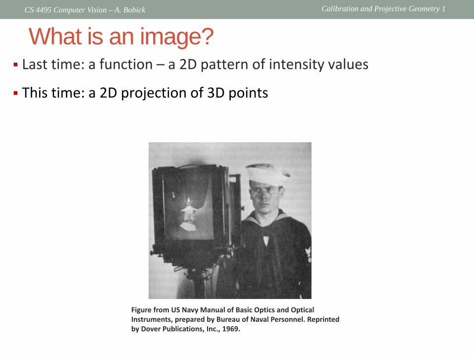
What is an image?
Figure from US Navy Manual of Basic Optics and Optical Instruments, prepared by Bureau of Naval Personnel. Reprinted by Dover Publications, Inc., 1969.
Last time: a function – a 2D pattern of intensity values
This time: a 2D projection of 3D points
Calibration and Projective Geometry 1 CS 4495 Computer Vision – A. Bobick
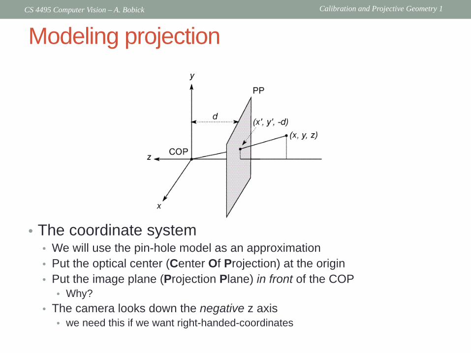
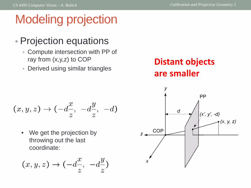
Modeling projection
• The coordinate system • We will use the pin-hole model as an approximation • Put the optical center (Center Of Projection) at the origin • Put the image plane (Projection Plane) in front of the COP
• Why? • The camera looks down the negative z axis
• we need this if we want right-handed-coordinates
Calibration and Projective Geometry 1 CS 4495 Computer Vision – A. Bobick
Modeling projection • Projection equations
• Compute intersection with PP of ray from (x,y,z) to COP
• Derived using similar triangles
• We get the projection by throwing out the last coordinate:
Distant objects are smaller
Calibration and Projective Geometry 1 CS 4495 Computer Vision – A. Bobick
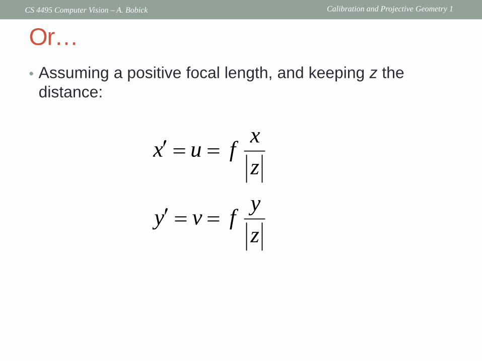
Or… • Assuming a positive focal length, and keeping z the
distance:
xx u fzyy v fz
′ = =
′ = =
Calibration and Projective Geometry 1 CS 4495 Computer Vision – A. Bobick
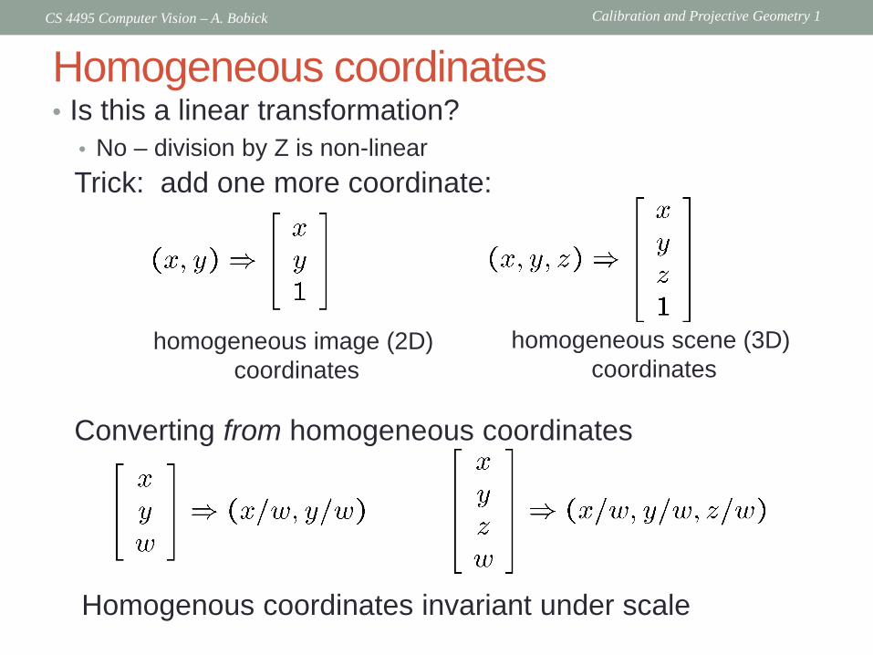
Homogeneous coordinates • Is this a linear transformation?
• No – division by Z is non-linear
Trick: add one more coordinate:
homogeneous image (2D) coordinates
homogeneous scene (3D) coordinates
Converting from homogeneous coordinates
Homogenous coordinates invariant under scale
Calibration and Projective Geometry 1 CS 4495 Computer Vision – A. Bobick
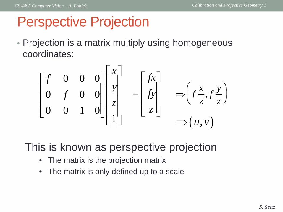
Perspective Projection • Projection is a matrix multiply using homogeneous
coordinates:
This is known as perspective projection • The matrix is the projection matrix • The matrix is only defined up to a scale
S. Seitz
( ),u v⇒
0 0 00 0 00 0 1 0
1
xf
yf
z
fxfyz
=
⇒ f xz
, f yz
Calibration and Projective Geometry 1 CS 4495 Computer Vision – A. Bobick
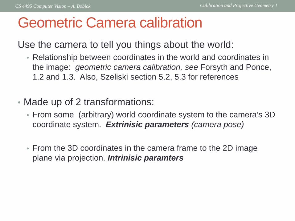
Geometric Camera calibration Use the camera to tell you things about the world:
• Relationship between coordinates in the world and coordinates in the image: geometric camera calibration, see Forsyth and Ponce, 1.2 and 1.3. Also, Szeliski section 5.2, 5.3 for references
• Made up of 2 transformations: • From some (arbitrary) world coordinate system to the camera’s 3D
coordinate system. Extrinisic parameters (camera pose)
• From the 3D coordinates in the camera frame to the 2D image plane via projection. Intrinisic paramters
Calibration and Projective Geometry 1 CS 4495 Computer Vision – A. Bobick
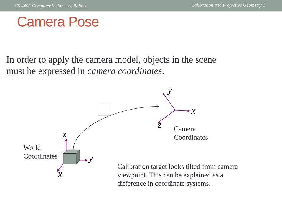
Camera Pose
In order to apply the camera model, objects in the scene must be expressed in camera coordinates.
World Coordinates
Camera Coordinates
Calibration target looks tilted from camera viewpoint. This can be explained as a difference in coordinate systems.
This image cannot currently be displayed.
y
x
z
z
x
y
Calibration and Projective Geometry 1 CS 4495 Computer Vision – A. Bobick
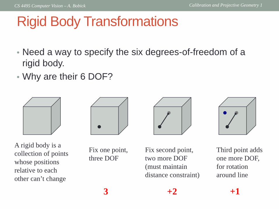
Rigid Body Transformations
• Need a way to specify the six degrees-of-freedom of a rigid body.
• Why are their 6 DOF?
A rigid body is a collection of points whose positions relative to each other can’t change
Fix one point, three DOF
3
Fix second point, two more DOF (must maintain distance constraint)
+2
Third point adds one more DOF, for rotation around line
+1
Calibration and Projective Geometry 1 CS 4495 Computer Vision – A. Bobick
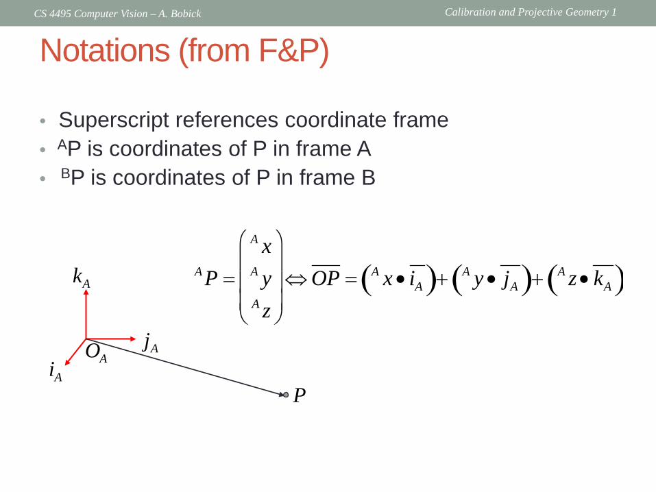
Notations (from F&P)
• Superscript references coordinate frame • AP is coordinates of P in frame A • BP is coordinates of P in frame B
A P =
A xA yA z
⇔ OP = A x • iA( )+ A y • jA( )+ A z • kA( )
kA
jA
iA
OA
P
Calibration and Projective Geometry 1 CS 4495 Computer Vision – A. Bobick
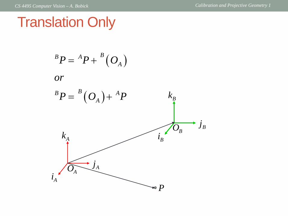
Translation Only
kA
jA
iA
kB
jB
iB
OB
OA
( )
( )
BB AA
BB AA
P P Oor
P O P
= +
= +
P
Calibration and Projective Geometry 1 CS 4495 Computer Vision – A. Bobick
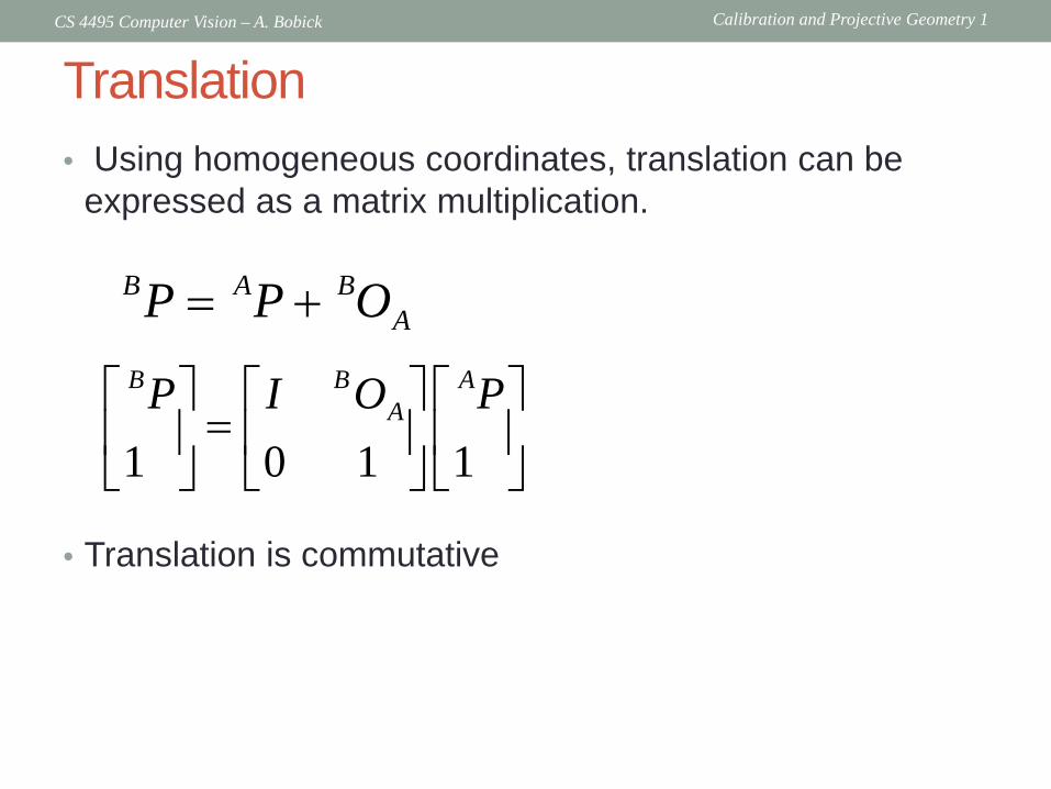
Translation • Using homogeneous coordinates, translation can be
expressed as a matrix multiplication.
• Translation is commutative
B A BAP P O= +
1 0 1 1
B B AAP I O P
=
Calibration and Projective Geometry 1 CS 4495 Computer Vision – A. Bobick
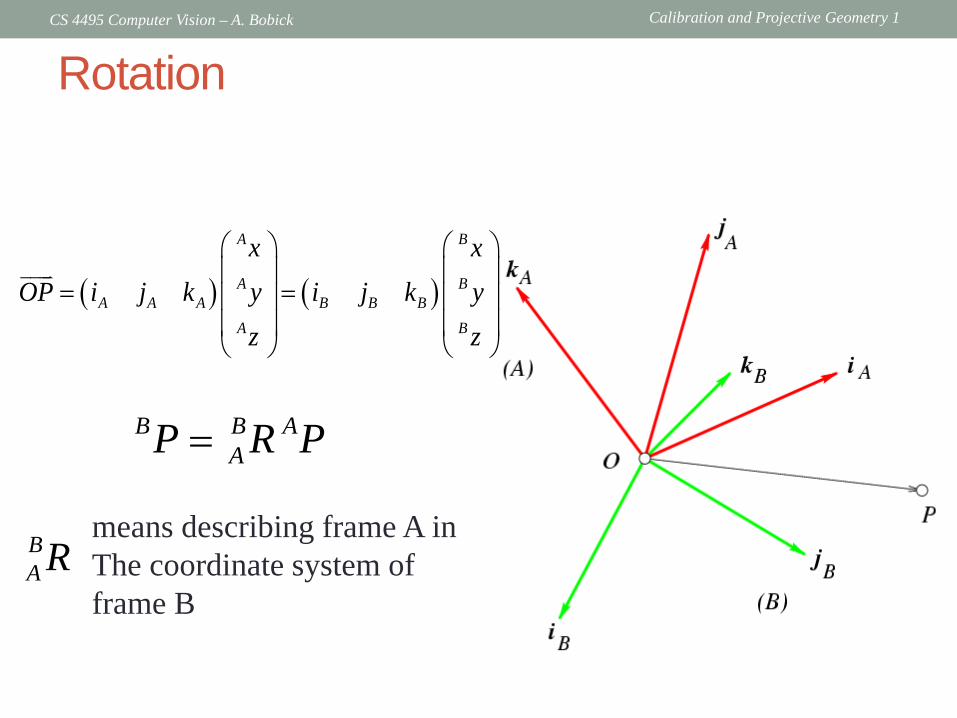
Rotation
( ) ( )
A B
A BA A A B B B
A B
x xOP i j k y i j k y
z z
= =
B B AAP R P=
BA R
means describing frame A in The coordinate system of frame B
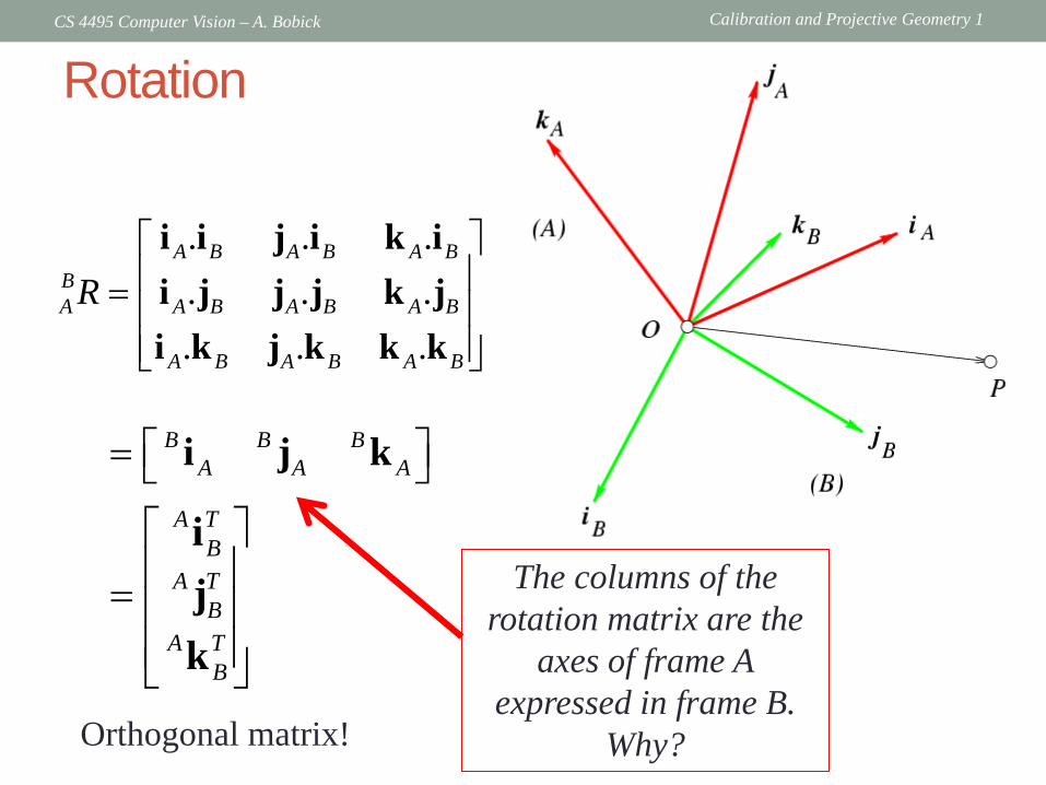
Calibration and Projective Geometry 1 CS 4495 Computer Vision – A. Bobick
Rotation
. . .
. . .. . .
A B A B A BBA A B A B A B
A B A B A B
R =
i i j i k ii j j j k ji k j k k k
B B BA A A = i j k
Orthogonal matrix!
A TB
A TB
A TB
=
ijk
The columns of the rotation matrix are the
axes of frame A expressed in frame B.
Why?
Calibration and Projective Geometry 1 CS 4495 Computer Vision – A. Bobick
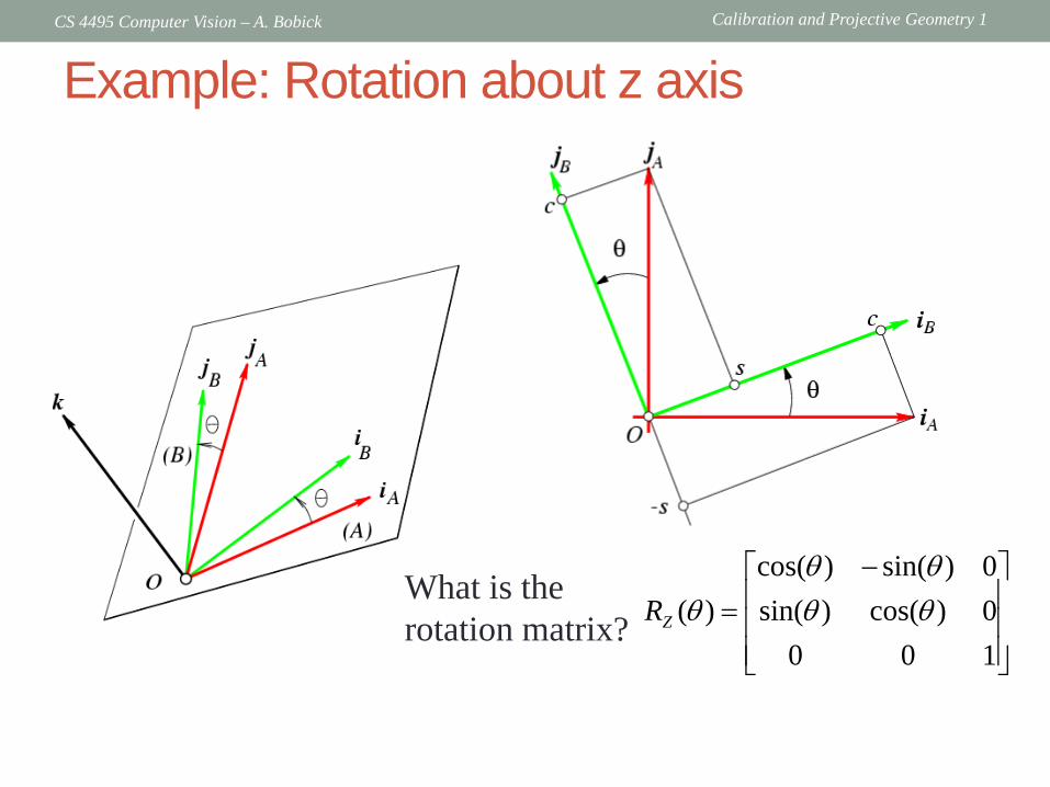
Example: Rotation about z axis
What is the rotation matrix?
−=
1000)cos()sin(0)sin()cos(
)( θθθθ
θZR
Calibration and Projective Geometry 1 CS 4495 Computer Vision – A. Bobick
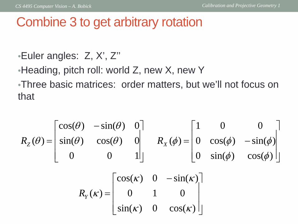
Combine 3 to get arbitrary rotation
•Euler angles: Z, X’, Z’’ •Heading, pitch roll: world Z, new X, new Y •Three basic matrices: order matters, but we’ll not focus on that
−=
1000)cos()sin(0)sin()cos(
)( θθθθ
θZR
−=
)cos()sin(0)sin()cos(0
001)(
φφφφφXR
−=
)cos(0)sin(010
)sin(0)cos()(
κκ
κκκYR
Calibration and Projective Geometry 1 CS 4495 Computer Vision – A. Bobick
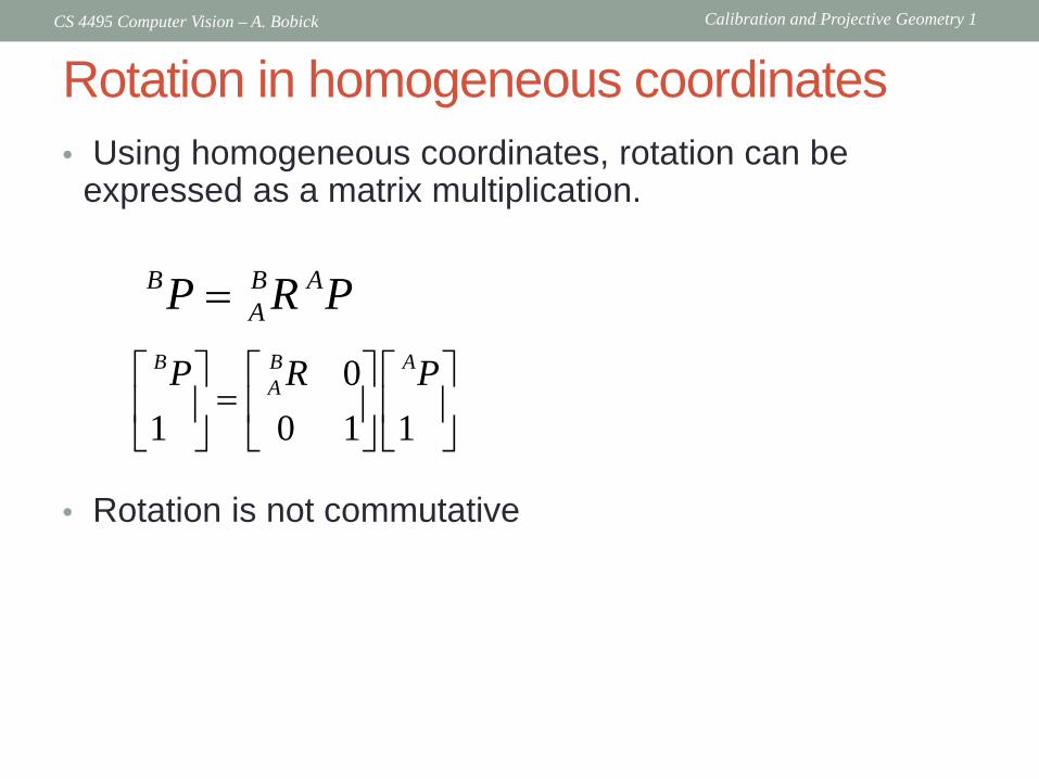
Rotation in homogeneous coordinates • Using homogeneous coordinates, rotation can be
expressed as a matrix multiplication.
• Rotation is not commutative
B B AAP R P=
01 0 1 1
B B AAP R P
=
Calibration and Projective Geometry 1 CS 4495 Computer Vision – A. Bobick
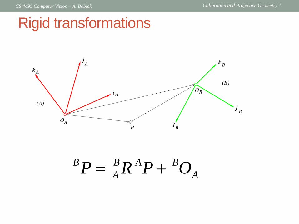
Rigid transformations
B B A BA AP R P O= +
Calibration and Projective Geometry 1 CS 4495 Computer Vision – A. Bobick
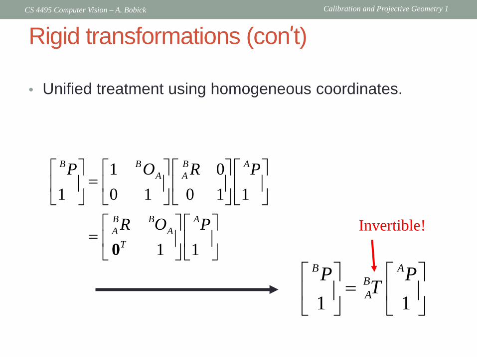
Rigid transformations (con’t)
• Unified treatment using homogeneous coordinates.
1 01 0 1 0 1 1
1 1
B B B AA A
B B AA A
T
P O R P
R O P
=
= 0
1 1
B ABA
P PT
=
Invertible!
Calibration and Projective Geometry 1 CS 4495 Computer Vision – A. Bobick
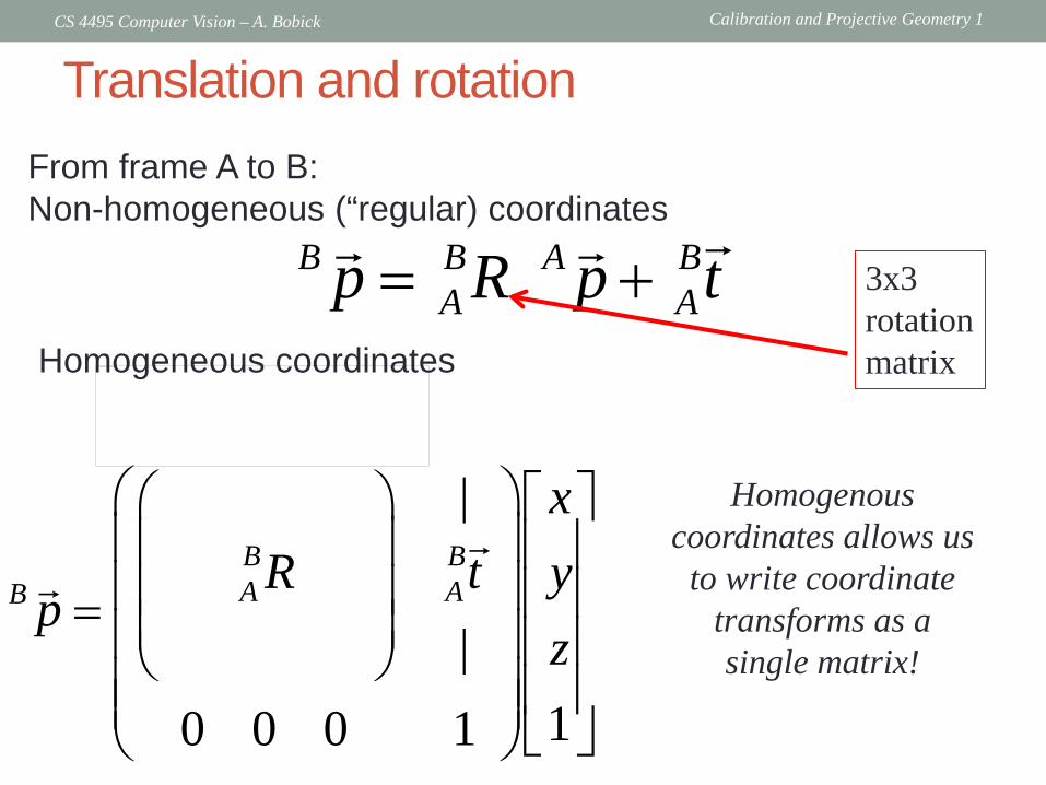
Translation and rotation From frame A to B: Non-homogeneous (“regular) coordinates
B B A BA Ap R p t= +
|
|10 0 0 1
B BA AB
xR t y
pz
=
This image cannot currently be displayed.Homogeneous coordinates
3x3 rotation matrix
Homogenous coordinates allows us
to write coordinate transforms as a single matrix!

Calibration and Projective Geometry 1 CS 4495 Computer Vision – A. Bobick
From World to Camera
C C W CW Wp R p t= +
Non-homogeneous coordinates
Homogeneous coordinates
|
|0 0 0 1
C C C WW Wp R t p
− − − − − = − − −
From world to camera is the extrinsic parameter matrix (4x4)
(sometimes 3x4 if using for next step in projection – not worrying about inversion)
Translation from world to camera frame
Rotation from world to camera frame
Point in world frame
Point in camera frame
Calibration and Projective Geometry 1 CS 4495 Computer Vision – A. Bobick
Now from Camera 3D to Image…
Calibration and Projective Geometry 1 CS 4495 Computer Vision – A. Bobick
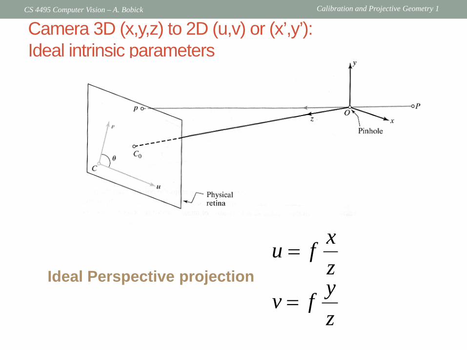
Camera 3D (x,y,z) to 2D (u,v) or (x’,y’): Ideal intrinsic parameters
zyfvzxfu
=
=Ideal Perspective projection
Calibration and Projective Geometry 1 CS 4495 Computer Vision – A. Bobick
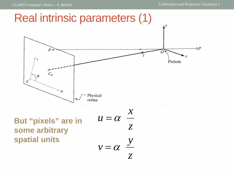
Real intrinsic parameters (1)
xuzyvz
α
α
=
=
But “pixels” are in some arbitrary spatial units
Calibration and Projective Geometry 1 CS 4495 Computer Vision – A. Bobick
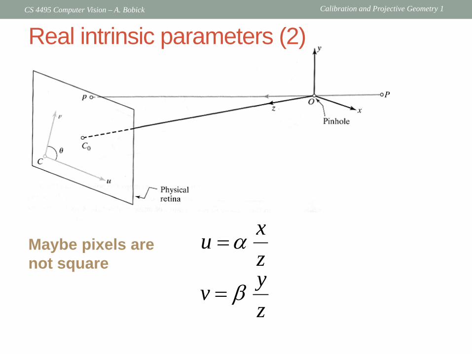
Real intrinsic parameters (2)
zyvzxu
β
α
=
=Maybe pixels are not square
Calibration and Projective Geometry 1 CS 4495 Computer Vision – A. Bobick
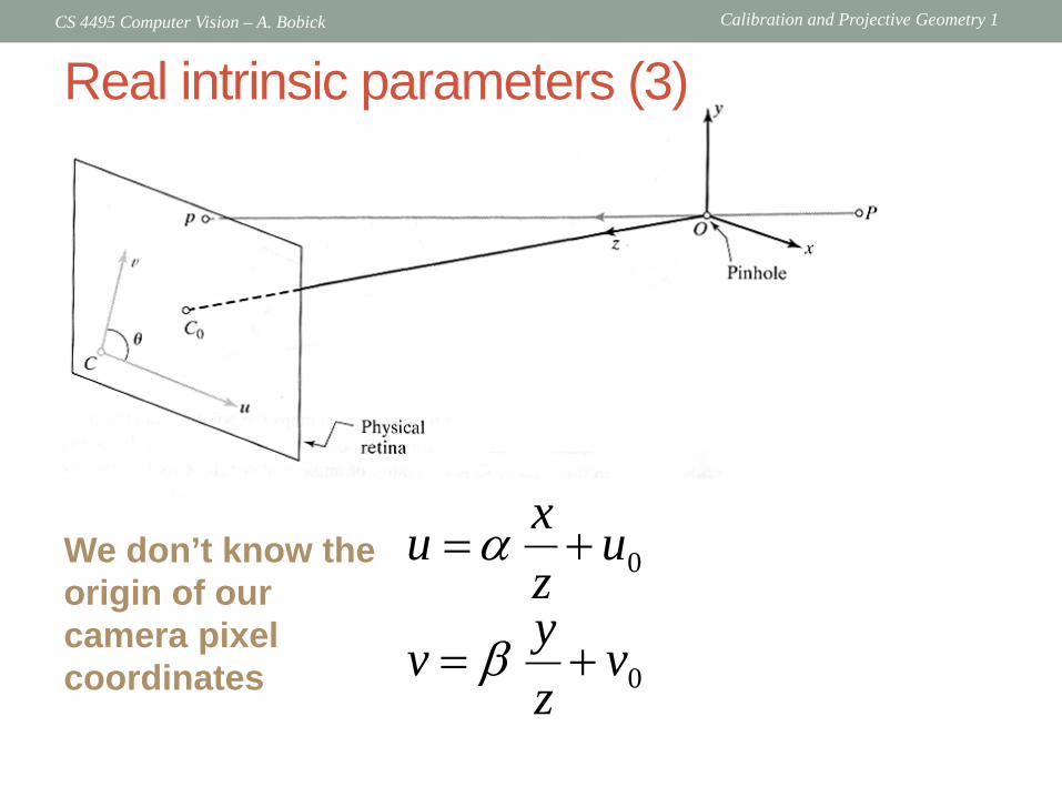
Real intrinsic parameters (3)
0
0
vzyv
uzxu
+=
+=
β
αWe don’t know the origin of our camera pixel coordinates
Calibration and Projective Geometry 1 CS 4495 Computer Vision – A. Bobick
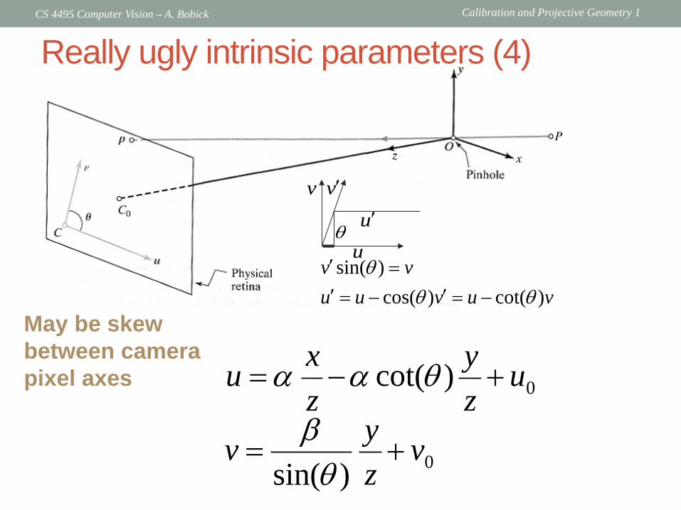
Really ugly intrinsic parameters (4)
0
0
)sin(
)cot(
vzyv
uzy
zxu
+=
+−=
θβ
θαα
May be skew between camera pixel axes
v
θu
v′ u′
vuvuuvv
)cot()cos()sin(
θθθ
−=′−=′=′
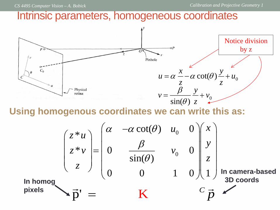
Calibration and Projective Geometry 1 CS 4495 Computer Vision – A. Bobick
p' K C p=
Intrinsic parameters, homogeneous coordinates
0
0
)sin(
)cot(
vzyv
uzy
zxu
+=
+−=
θβ
θαα
0
0
cot( ) 0** 0 0
sin( )0 0 1 0 1
xuz uy
z v vz
z
α α θβ
θ
− =
Using homogenous coordinates we can write this as:
In camera-based 3D coords In homog
pixels
Notice division by z
Calibration and Projective Geometry 1 CS 4495 Computer Vision – A. Bobick
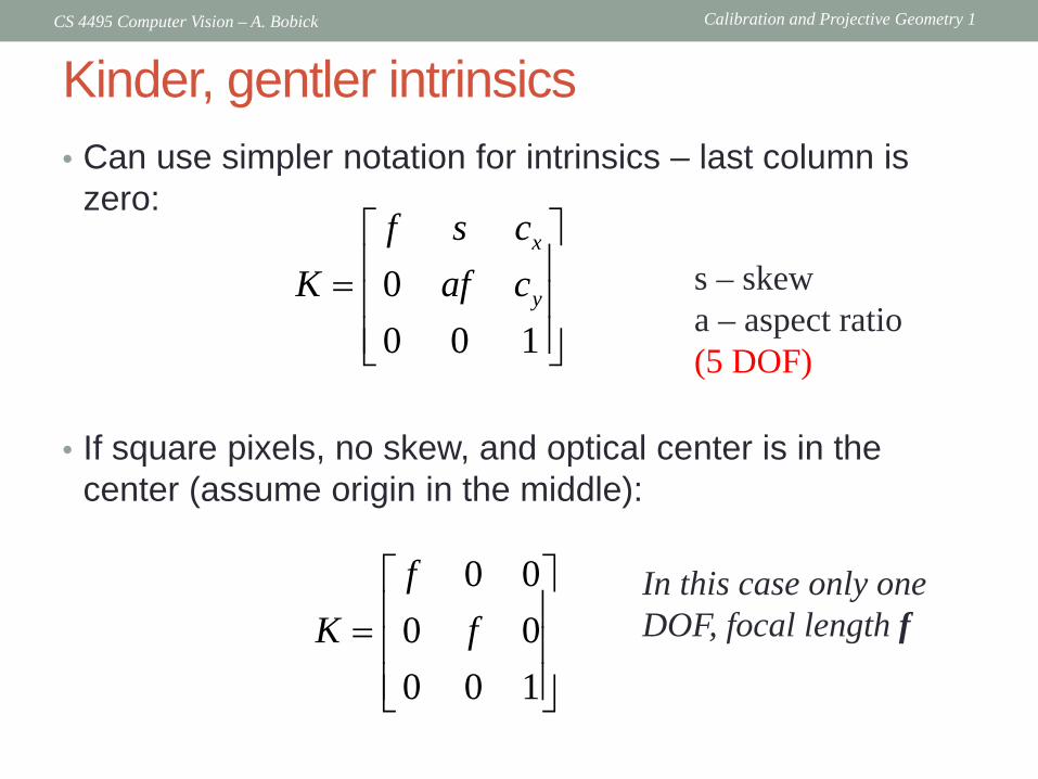
Kinder, gentler intrinsics • Can use simpler notation for intrinsics – last column is
zero:
• If square pixels, no skew, and optical center is in the center (assume origin in the middle):
00 0 1
x
y
f s cK af c
=
s – skew a – aspect ratio (5 DOF)
0 00 00 0 1
fK f
=
In this case only one DOF, focal length f
Calibration and Projective Geometry 1 CS 4495 Computer Vision – A. Bobick
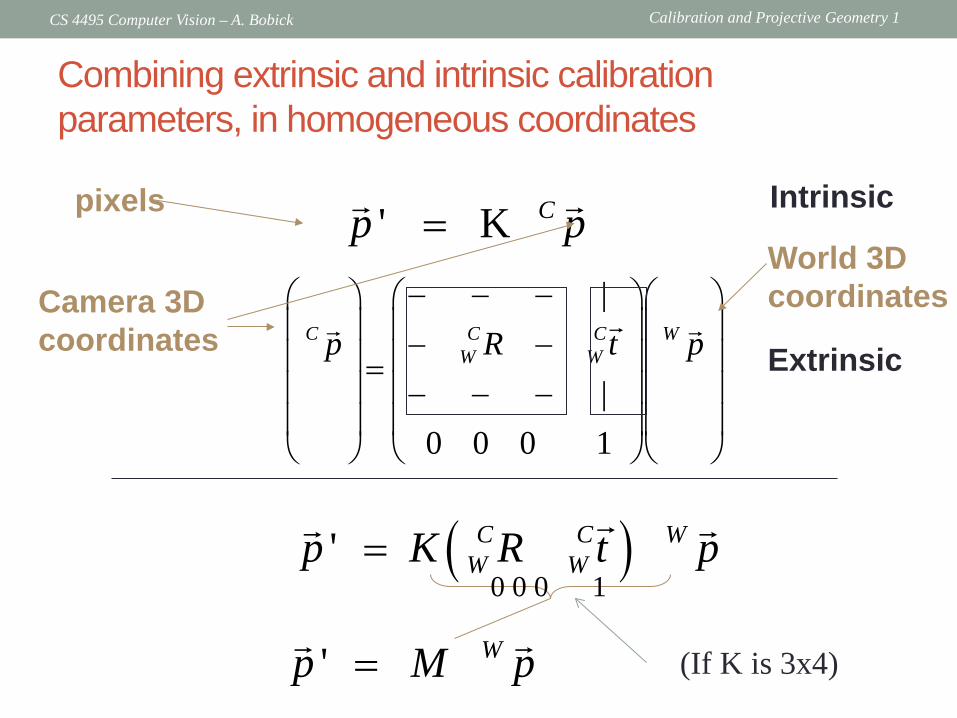
Combining extrinsic and intrinsic calibration parameters, in homogeneous coordinates
( )' C C WW Wp K R t p=
' K Cp p=
' Wp M p=
Intrinsic
Extrinsic
|
|0 0 0 1
C C C WW Wp R t p
− − − − − = − − −
World 3D coordinates Camera 3D
coordinates
pixels
0 0 0 1
(If K is 3x4)
Calibration and Projective Geometry 1 CS 4495 Computer Vision – A. Bobick
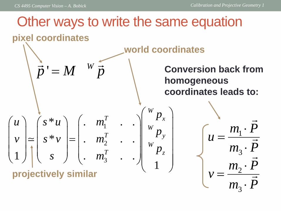
Other ways to write the same equation
1
2
3
* . . .* . . .
1 . . .1
WT x
WT y
WT z
pu s u m
pv s v m
ps m
=
' Wp M p=
pixel coordinates world coordinates
Conversion back from homogeneous coordinates leads to:
PmPmv
PmPmu
⋅⋅
=
⋅⋅
=
3
2
3
1
projectively similar
Calibration and Projective Geometry 1 CS 4495 Computer Vision – A. Bobick
Projection equation
• The projection matrix models the cumulative effect of all parameters • Useful to decompose into a series of operations
* * * ** * * ** * * *
1
Xsx
Ysy
Zs
= =
x MX
3 1 3 13 3 3 3
1 3 1 3
' 1 0 0 00 ' 0 1 0 0
1 10 0 1 0 0 1 0
cx xx x
cx x
f s xaf y
=
00 0R I TM
projection intrinsics rotation translation
identity matrix
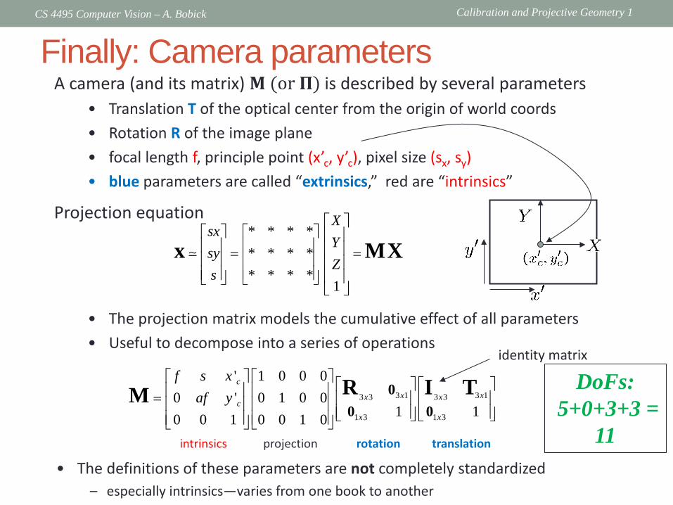
Finally: Camera parameters A camera (and its matrix) 𝐌 (or 𝚷) is described by several parameters
• Translation T of the optical center from the origin of world coords • Rotation R of the image plane • focal length f, principle point (x’c, y’c), pixel size (sx, sy) • blue parameters are called “extrinsics,” red are “intrinsics”
• The definitions of these parameters are not completely standardized – especially intrinsics—varies from one book to another
DoFs: 5+0+3+3 =
11
Calibration and Projective Geometry 1 CS 4495 Computer Vision – A. Bobick
Calibration • How to determine M (or 𝚷)?
Calibration and Projective Geometry 1 CS 4495 Computer Vision – A. Bobick
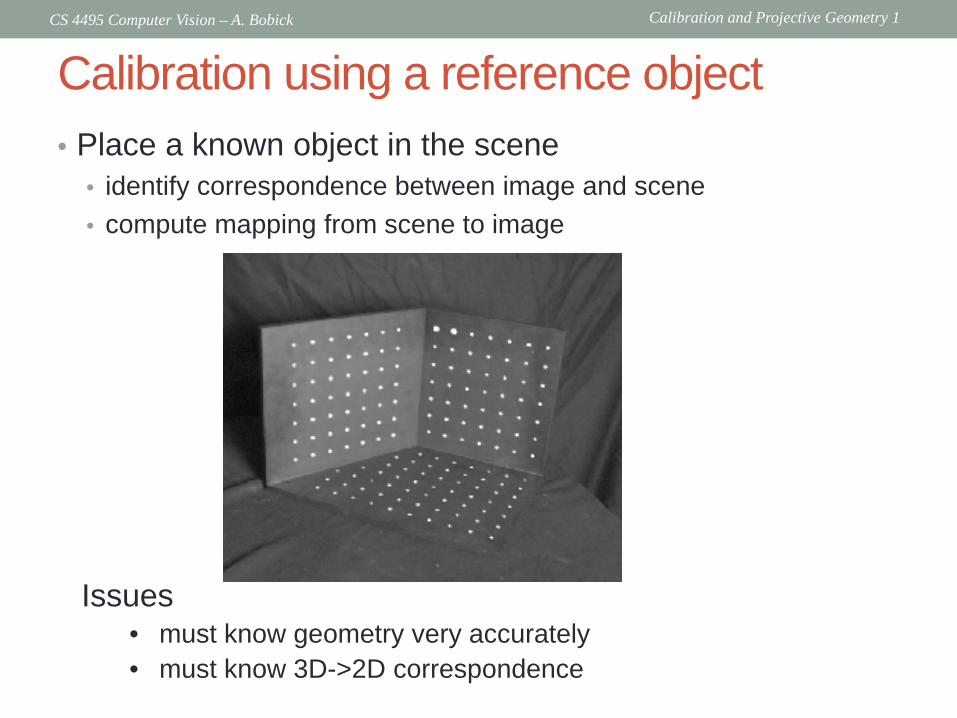
Calibration using a reference object • Place a known object in the scene
• identify correspondence between image and scene • compute mapping from scene to image
Issues • must know geometry very accurately • must know 3D->2D correspondence
Calibration and Projective Geometry 1 CS 4495 Computer Vision – A. Bobick
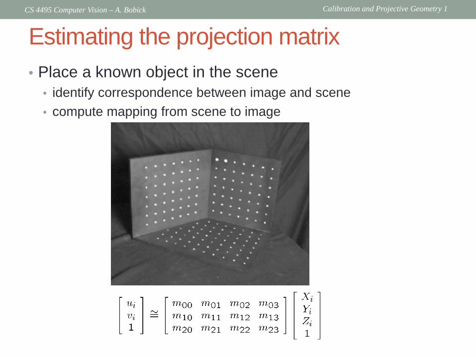
Estimating the projection matrix • Place a known object in the scene
• identify correspondence between image and scene • compute mapping from scene to image
Calibration and Projective Geometry 1 CS 4495 Computer Vision – A. Bobick
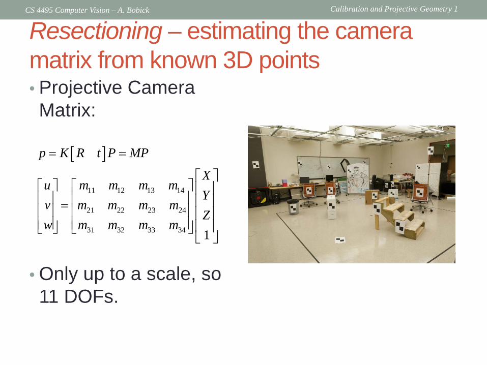
Resectioning – estimating the camera matrix from known 3D points • Projective Camera Matrix:
• Only up to a scale, so 11 DOFs.
[ ]
11 12 13 14
21 22 23 24
31 32 33 34 1
p K R t P MP
Xu m m m m
Yv m m m m
Zw m m m m
= =
=
Calibration and Projective Geometry 1 CS 4495 Computer Vision – A. Bobick
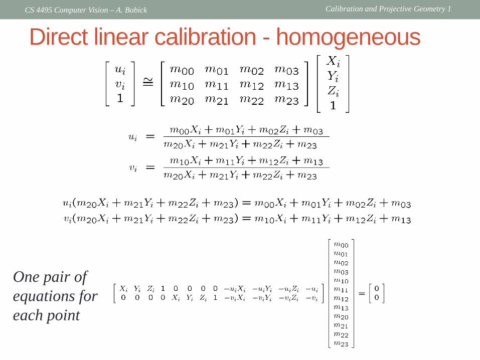
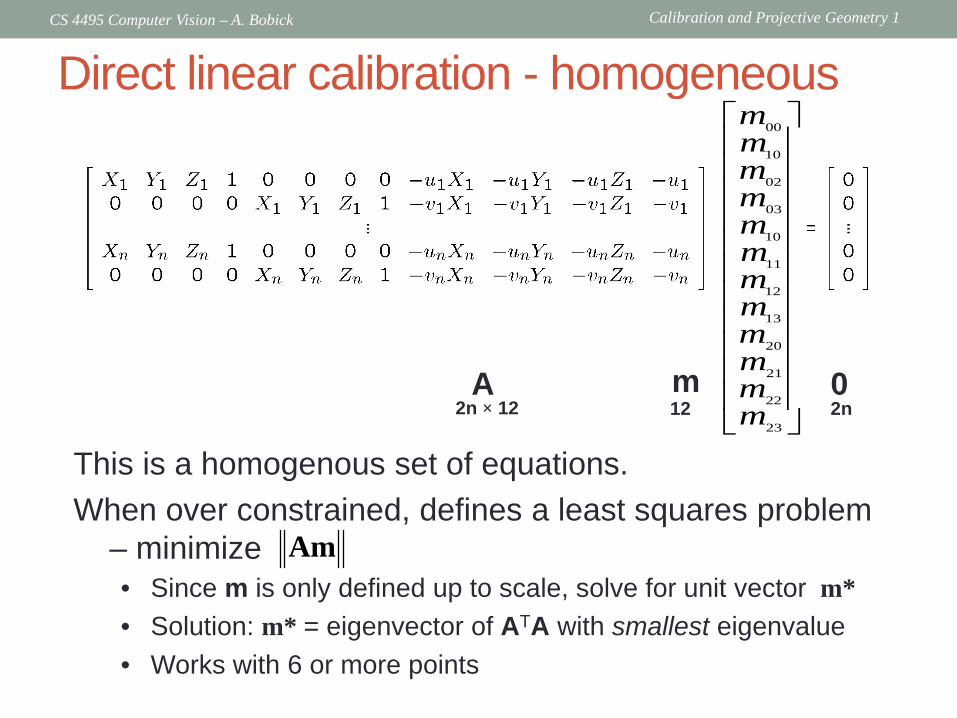
Direct linear calibration - homogeneous
One pair of equations for each point
Calibration and Projective Geometry 1 CS 4495 Computer Vision – A. Bobick
Direct linear calibration - homogeneous
This is a homogenous set of equations. When over constrained, defines a least squares problem
– minimize
A m 0 2n × 12 12 2n
• Since m is only defined up to scale, solve for unit vector m* • Solution: m* = eigenvector of ATA with smallest eigenvalue • Works with 6 or more points
Am
00
10
02
03
10
11
12
13
20
21
22
23
mmmmmmmmmmmm
Calibration and Projective Geometry 1 CS 4495 Computer Vision – A. Bobick
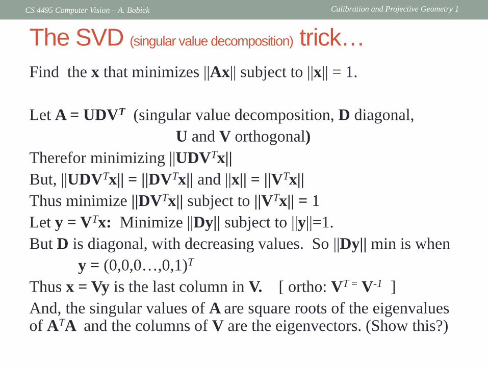
The SVD (singular value decomposition) trick… Find the x that minimizes ||Ax|| subject to ||x|| = 1. Let A = UDVT (singular value decomposition, D diagonal, U and V orthogonal) Therefor minimizing ||UDVTx|| But, ||UDVTx|| = ||DVTx|| and ||x|| = ||VTx|| Thus minimize ||DVTx|| subject to ||VTx|| = 1 Let y = VTx: Minimize ||Dy|| subject to ||y||=1. But D is diagonal, with decreasing values. So ||Dy|| min is when y = (0,0,0…,0,1)T
Thus x = Vy is the last column in V. [ ortho: VT = V-1 ] And, the singular values of A are square roots of the eigenvalues of ATA and the columns of V are the eigenvectors. (Show this?)

Calibration and Projective Geometry 1 CS 4495 Computer Vision – A. Bobick
Direct linear calibration - inhomogeneous • Another approach: 1 in lower r.h. corner for 11 d.o.f
• Now “regular” least squares since there is a non-variable
term in the equations:
00 01 02 03
10 11 12 13
20 21 221 11
Xu m m m m
Yv m m m m
Zm m m
Dangerous if m23 is really
zero!
Calibration and Projective Geometry 1 CS 4495 Computer Vision – A. Bobick
Direct linear calibration (transformation) • Advantage:
• Very simple to formulate and solve. Can be done, say, on a problem set
• These methods are referred to as “algebraic error” minimization.
• Disadvantages: • Doesn’t directly tell you the camera parameters (more in a bit) • Doesn’t model radial distortion • Hard to impose constraints (e.g., known focal length) • Doesn’t minimize the right error function
For these reasons, nonlinear methods are preferred • Define error function E between projected 3D points and image positions
– E is nonlinear function of intrinsics, extrinsics, radial distortion
• Minimize E using nonlinear optimization techniques – e.g., variants of Newton’s method (e.g., Levenberg Marquart)
Calibration and Projective Geometry 1 CS 4495 Computer Vision – A. Bobick
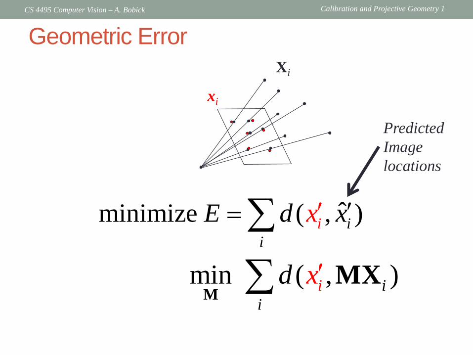
Geometric Error
ˆminimize ( , )ii
iE d x x′ ′= ∑min ( , )i
iixd ′∑M
MX
Predicted Image locations
Xi
xi
Calibration and Projective Geometry 1 CS 4495 Computer Vision – A. Bobick
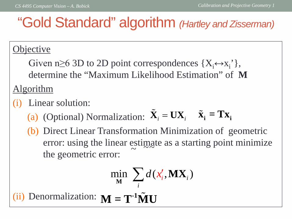
“Gold Standard” algorithm (Hartley and Zisserman)
Objective Given n≥6 3D to 2D point correspondences {Xi↔xi’},
determine the “Maximum Likelihood Estimation” of M Algorithm (i) Linear solution:
(a) (Optional) Normalization: (b) Direct Linear Transformation Minimization of geometric
error: using the linear estimate as a starting point minimize the geometric error:
(ii) Denormalization:
i i=X UX
i ix = Tx
-1M = T MU
~ ~ ~
min ( , )ii
ixd ′∑MMX
Calibration and Projective Geometry 1 CS 4495 Computer Vision – A. Bobick
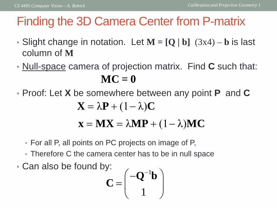
Finding the 3D Camera Center from P-matrix • Slight change in notation. Let M = [Q | b] (3x4) – b is last
column of M • Null-space camera of projection matrix. Find C such that:
• Proof: Let X be somewhere between any point P and C
• For all P, all points on PC projects on image of P, • Therefore C the camera center has to be in null space
• Can also be found by:
MC = 0
λ (1 λ)= + −X P Cλ (1 λ)= = + −x MX MP MC
1
1
− −=
Q bC
Calibration and Projective Geometry 1 CS 4495 Computer Vision – A. Bobick
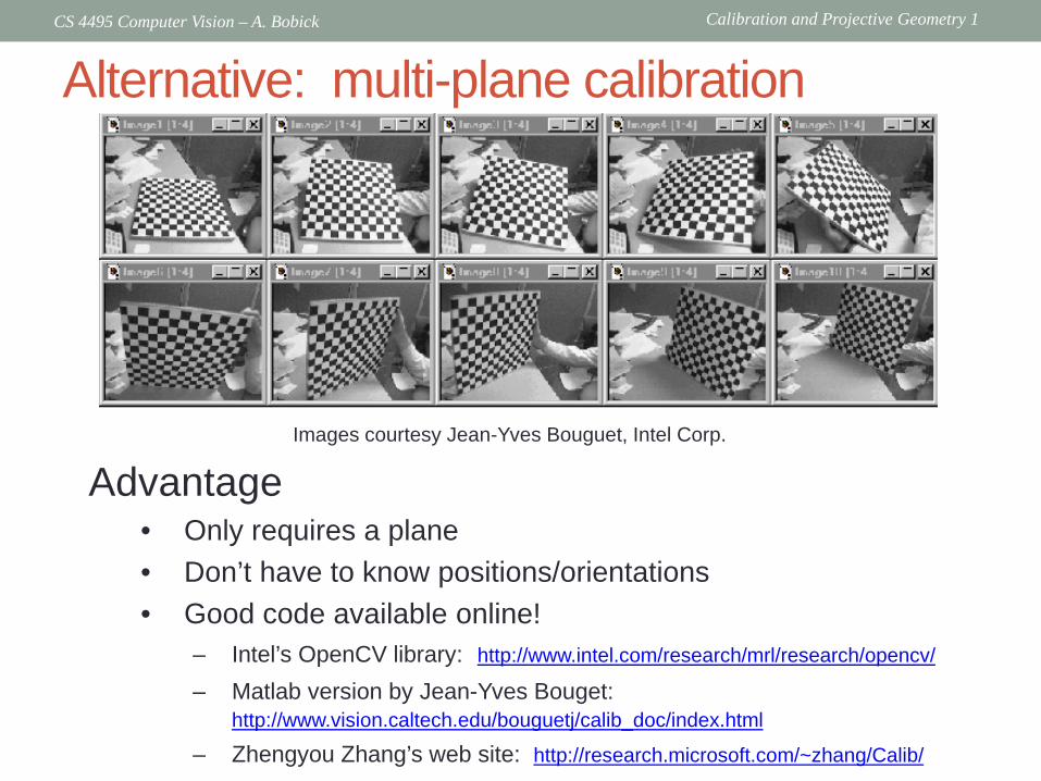
Alternative: multi-plane calibration
Images courtesy Jean-Yves Bouguet, Intel Corp.
Advantage • Only requires a plane • Don’t have to know positions/orientations • Good code available online!
– Intel’s OpenCV library: http://www.intel.com/research/mrl/research/opencv/
– Matlab version by Jean-Yves Bouget: http://www.vision.caltech.edu/bouguetj/calib_doc/index.html
– Zhengyou Zhang’s web site: http://research.microsoft.com/~zhang/Calib/