cs 450: computer graphics ray tracing -...
TRANSCRIPT

CS 450: COMPUTER GRAPHICS
RAY TRACINGSPRING 2016
DR. MICHAEL J. REALE

RENDERING IMAGES
• Let’s say we have a scene of 3D objects
• We want to render this to a 2D raster image
• In general, there are two ways we can do this:
• Object-order rendering
• For each OBJECT find pixels that object affects
• Often used for real-time rendering
• Image-ordering rendering
• For each PIXEL find all objects that affect this pixel
• Often used for non-real-time rendering
We’ve got this… …and we want this

RAY TRACING
• We’re going to talk about ray tracing
• Form of image-order rendering
• Advantages:
• High-quality images
• Easy to compute:
• Shadows
• Reflections
• Refraction
• Disadvantages:
• Generally pretty slow

BASIC RAY-TRACING ALGORITHM
BASIC IDEA
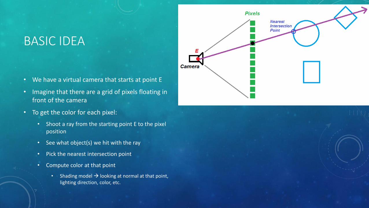
• We have a virtual camera that starts at point E
• Imagine that there are a grid of pixels floating in front of the camera
• To get the color for each pixel:
• Shoot a ray from the starting point E to the pixel position
• See what object(s) we hit with the ray
• Pick the nearest intersection point
• Compute color at that point
• Shading model looking at normal at that point, lighting direction, color, etc.

THREE BASIC STEPS
• This means we have three basic steps:
• Ray generation
• Compute viewing ray for each pixel
• Ray intersection
• Find closest intersection point among all objects in scene
• This step why raytracers are generally slow
• Shading
• Compute pixel color based on results of ray intersection

PERSPECTIVE

3D TO 2D
• Our first question is how our camera will project the 3D world onto a 2D image?
• Old problem: artists had been working on this one for centuries
• Simplest approach:
• Distance from camera doesn’t matter
• Only care where it is in terms of left/right and up/down
• More realistic approach:
• Take perspective into account things farther away should look smaller
https://static.greatbigcanvas.com/categories/medieval-art-11307.jpghttps://northierthanthou.files.wordpress.com/2012/12/renaissance-the-school-of-athens-classic-art-paitings-raphael-painter-rafael-philosophers-hd-wallpapers.jpg?w=762

PROJECTIONS
• Two most commonly used projection methods:
• Orthographic (or parallel)
• Perspective
• Note: when defining a projection, also define:
• Near plane = closer than near plane don’t render
• Far plane = beyond far plane don’t render
• Coupled with other aspects of camera, defines view volume
• Objects in view volume will be rendered
• Projection direction = direction our camera is pointed
Orthographic Perspective

ORTHOGRAPHIC PROJECTION
• Orthographic (or parallel)
• Move object along projection direction until you hit image plane
• Distance from image plane doesn’t change appearance
• Parallel lines remain parallel
• View volume = rectangular box

ORTHOGRAPHIC PROJECTION: PROS AND CONS
• Orthographic (or parallel)
• Advantages:
• Good for mechanical/architectural drawings
• Size of objects remains the same, no matter how far away they are
• Parallel lines preserved
• Disadvantages:
• Not realistic effectively assumes multiple camera (eye) starting points
• In reality, just one (or two, with the human vision system)

PERSPECTIVE PROJECTION
• Perspective
• Single starting point (eye point) all objects project towards eye point
• Things look smaller when farther away
• View volume = truncated pyramid with rectangular base called view frustum

ASIDE: OBLIQUE PROJECTION
• If the image plane is NOT orthogonal to the project direction oblique projection
• Below: example of an oblique parallel projection

COMPUTING VIEWING RAYS
CREATING RAYS
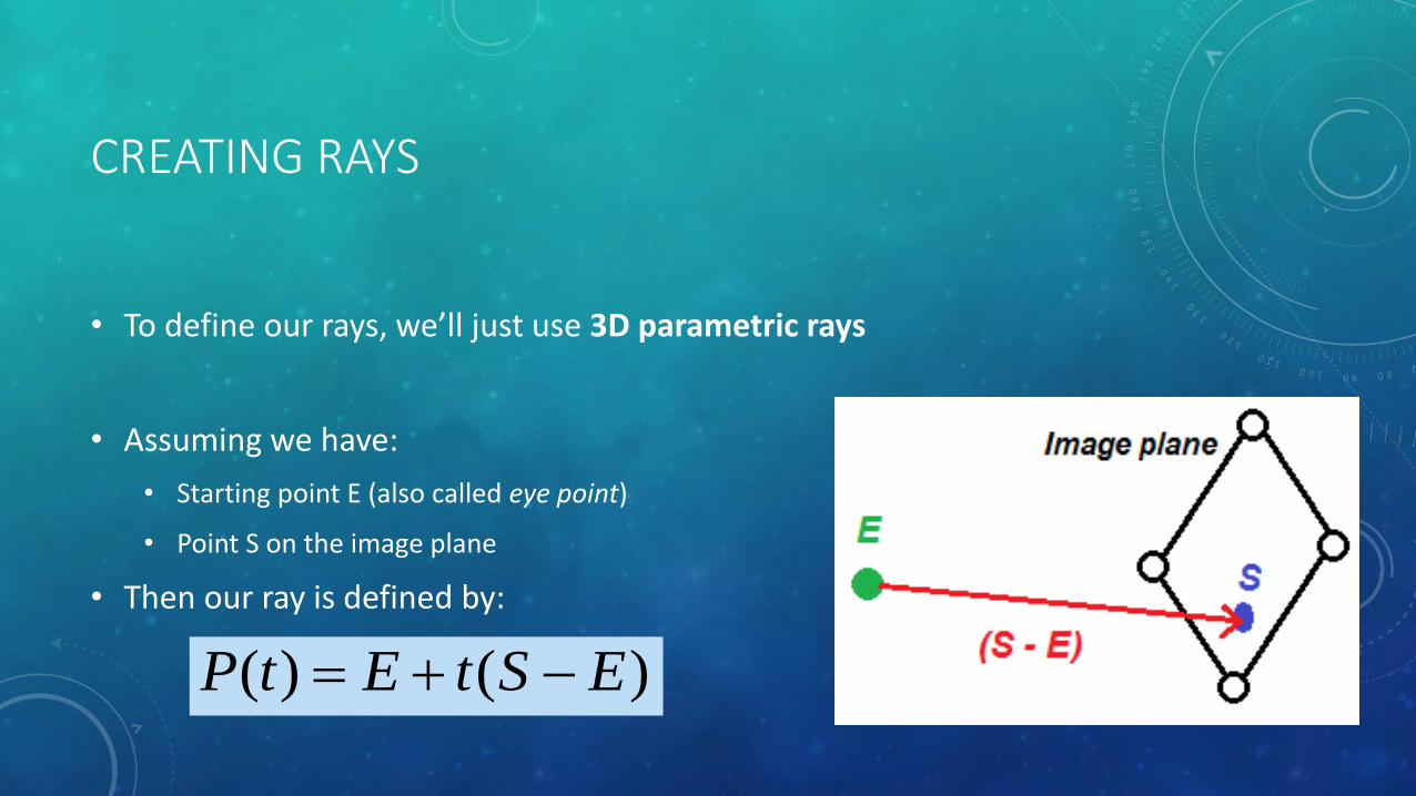
• To define our rays, we’ll just use 3D parametric rays
• Assuming we have:
• Starting point E (also called eye point)
• Point S on the image plane
• Then our ray is defined by:
)()( EStEtP

BEHIND BLUE EYES
• We know that:
• We also know that, if:
• Then P(t1) is closer to eye than P(t2)
• If (t < 0) “behind” the eye (shouldn’t be able to see item)
SP
EP
)1(
)0(
210 tt

CAMERA FRAME
• We need to find the S points
• E will be given to us, depending on the kind of projection
• To do this, we will look at things from the perspective of the camera frame
• Camera frame = orthonormal coordinate frame defined by the eye point E and three vectors:
• U points to camera’s RIGHT
• V points upward
• W points BACKWARD
• Remember: RIGHT-HAND RULE, so camera is actually looking along the –W axis!

GETTING THE IMAGE PLANE
• Based on the camera frame, we’ll construct our image plane
• We know:
• Right (U) and Up (V) directions for plane
• Assume we also know where the plane is centered
• How large is the plane?
• Usually define plane in terms of the following coordinates:
• r (right) max coordinate ALONG U axis (r > 0)
• l (left) min coordinate ALONG U axis (l < 0)
• t (top) max coordinate ALONG V axis (t > 0)
• b (bottom) min coordinate ALONG V axis (b < 0)

GETTING POINTS ON THE IMAGE PLANE
• We then need to define what points on the image plane correspond to our pixels
• If:
• nx = # of pixels in x
• ny = # of pixels of y
• To get the coordinates (u,v) for a given point (assuming that pixels are ACTUALLY centered on the 2D coordinates):
y
x
njbtbv
nilrlu
/)5.0)((
/)5.0)((

ORTHOGRAPHIC VIEWS
• For an orthographic view, all ray DIRECTIONS = -W
• Image plane centered at eye point E
• For each pixel:
• Compute u and v (previous slide)
• For oblique views all ray directions = d (some other direction)
vVuUE
W
point startingRay
direction Ray

PERSPECTIVE VIEWS
• For perspective views, all ray STARTING POINTS = E
• Image plane centered at (E - dW)
• d = image plane distance
• Sometimes loosely called focal length changing d does change field of view
• For each pixel:
• Compute u and v (two slides back)
• For oblique views use dD instead of -dW
E
dWvVuU
point startingRay
direction Ray

RAY-OBJECT INTERSECTION
FINDING OBJECTS
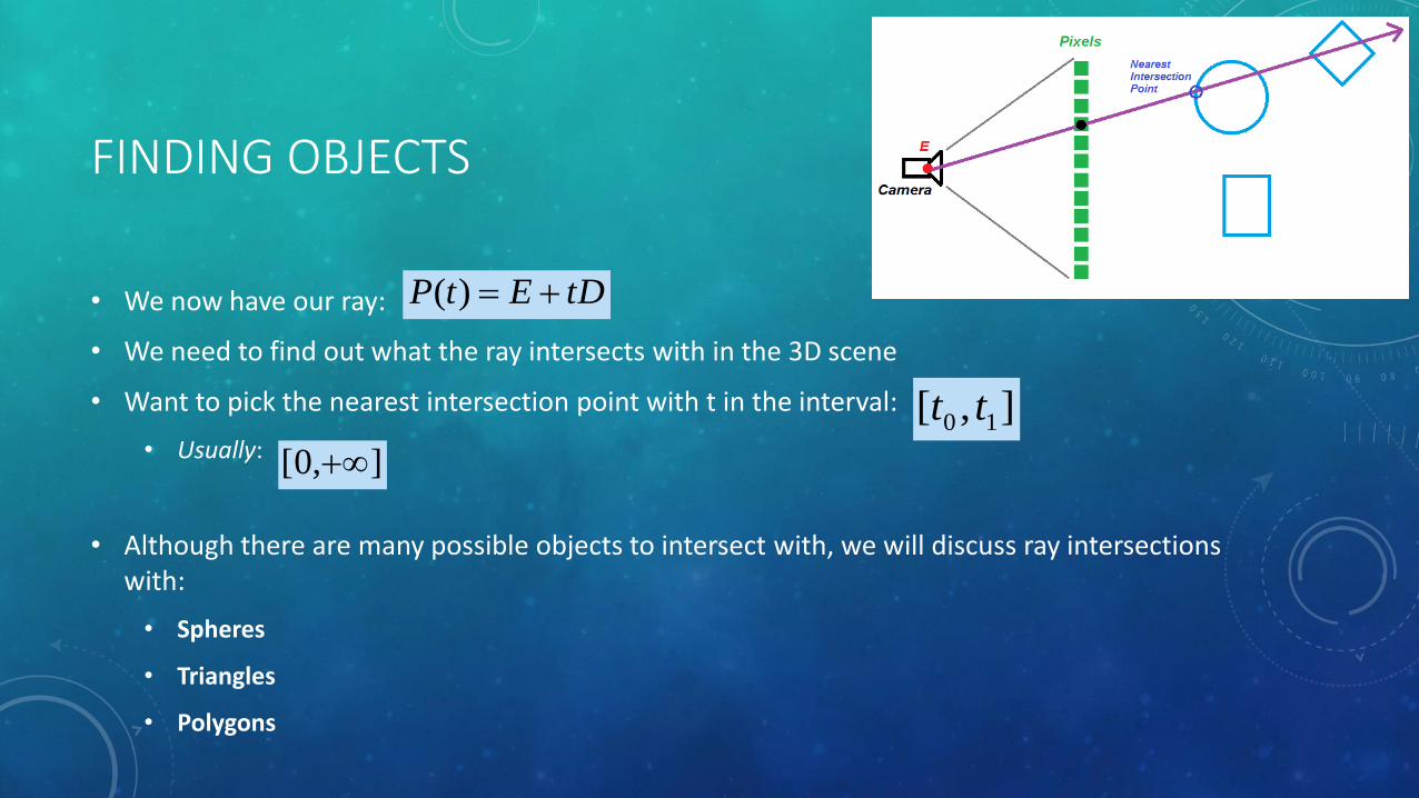
• We now have our ray:
• We need to find out what the ray intersects with in the 3D scene
• Want to pick the nearest intersection point with t in the interval:
• Usually:
• Although there are many possible objects to intersect with, we will discuss ray intersections with:
• Spheres
• Triangles
• Polygons
],[ 10 tt
],0[
tDEtP )(

RAY INTERSECTION WITH IMPLICIT SURFACE
• Here’s our ray again:
• Given an implicit surface:
• Intersection points = points on ray that satisfy the implicit equation:
• So we have to find values of t (if any) that satisfy the above equation.
tDEtP )(
0)( Pf
0)(0))(( tDEfortPf

RAY-SPHERE INTERSECTION

RAY-SPHERE INTERSECTION
• Here’s our implicit equation (in vector form) for a sphere:
• Let’s plug in our ray for P:
0)()()( 2 rCPCPPf
tDEtP )(
0)()()( 2 rCtDECtDEPf
Our Ray

RAY-SPHERE INTERSECTION
• Rearranging terms:
22
22
22
2
2
)()())((2)(
)()(2)()(2)(
)()()(2)(2)(2)(
)()()()()()()()()(
)()(
rCECEtCEDtDD
rCCECEECDEDttDD
rCCEECDtECEDttDD
rCCCtDCEtDCtDtDtDEECEtDEE
rCtDECtDE

RAY-SPHERE INTERSECTION
• A closer look at our result:
• …reveal that this is a quadratic equation:
• …where:
0)()())((2)( 22 rCECEtCEDtDD
02 cbtat
2)()(
))((2
)(
rCECEc
CEDb
DDa

RAY-SPHERE INTERSECTION
• This means we can use the quadratic formula!
a
acbbt
2
42
)(2
))())(((4)))((2())((2 22
DD
rCECEDDCEDCEDt
2)()(
))((2
)(
rCECEc
CEDb
DDa

RAY-SPHERE INTERSECTION
• Cleaning things up a bit:
• If we look at the discriminant G:
• G > 0 TWO possible intersection points
• G = 0 ONE possible intersection point (grazing surface of sphere)
• G < 0 NO intersection
• In implementation, one should check the discriminant first before computing other terms
• In fact, if doing collision detection may only need to compute the discriminant!
)(
))())((())(())(( 22
DD
rCECEDDCEDCEDt

RAY-SPHERE INTERSECTION

RAY-SPHERE INTERSECTION: GEOMETRIC INTERPRETATION
• Let’s try to break this down geometrically…
• Vector going from center of circle TO eye point:
• Length of projection of (E-C) onto D:
• However, if we just wanted the adjacent side and assumed D was normalized:
• THAT SAID, note that (E-C) and D point in opposing directions, so the distance along D we ACTUALLY want is:
)(
))())((())(())(( 22
DD
rCECEDDCEDCEDt
)( CE
2
cos)()(
D
CED
DD
CED
cos)( CEp
p

RAY-SPHERE INTERSECTION: GEOMETRIC INTERPRETATION
• That said, our original formula:
• …becomes (also converting certain dot products to the lengths-squared):
)(
))())((())(())(( 22
DD
rCECEDDCEDCEDt
2
2222))((
D
rCEDpDpDt

RAY-SPHERE INTERSECTION: GEOMETRIC INTERPRETATION
• We can actually move the length of D outside of the square root:
2
2222))((
D
rCEDpDpDt
2
222 ))((
D
rCEpDpDt
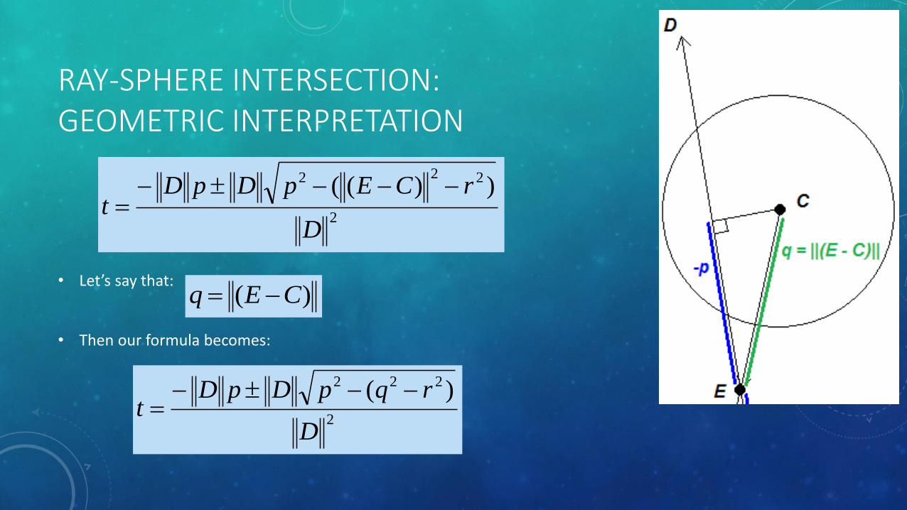
RAY-SPHERE INTERSECTION: GEOMETRIC INTERPRETATION
• Let’s say that:
• Then our formula becomes:
2
222 ))((
D
rCEpDpDt
)( CEq
2
222 )(
D
rqpDpDt

RAY-SPHERE INTERSECTION: GEOMETRIC INTERPRETATION
• Let’s look at the discriminant more closely:
• Rearranging it a bit:
• Because of the Pythagorean theorem:
• So, if we’re trying to get s2:
• SO, we are effectively getting the difference between r2 and s2:
)( 222 rqp
)( 222 qpr
222 spq
222 pqs
22
222
222
)(
)(
sr
pqr
qpr

RAY-SPHERE INTERSECTION: GEOMETRIC INTERPRETATION
• SO, when we are computing the discriminant G:22 srG
pointon intersecti no0
pointon intersecti ONE0
pointson intersecti TWO0
22
22
22
srG
srG
srG

RAY-SPHERE INTERSECTION: GEOMETRIC INTERPRETATION
• Let’s assume we have TWO intersection points (G > 0)
• It turns out that, if we look at ANOTHER right triangle, then:
• Which means that the square root of our discriminant gives us:
kksrG 222
222
222
srk
rks

RAY-SPHERE INTERSECTION: GEOMETRIC INTERPRETATION
• SO, plugging this value into our original formula (and canceling out the extra ||D||):
• In other words, in terms of ACTUAL geometric distance, we need to go along D by:
• (-p + k)
• (-p – k)
• …to get our two intersection points.
• HOWEVER, because D may not be normalized, we have to divide by the length of D
2
222 )(
D
rqpDpDt
D
kpt

RAY-TRIANGLE INTERSECTION

INTERSECTION WITH A TRIANGLE
• While there are many ways to do ray-triangle intersections, we will use:
• Barycentric coordinates
• A parametric plane containing the triangle
• Basically, all we need to store for this are the vertices of the triangle

RAY INTERSECTION WITH A PARAMETRIC SURFACE
• To intersect a ray with a parametric surface set up the following equations:
• Three unknowns (t,u,v) three equations
• Hopefully, we can solve this analytically, but in the worst case we can throw numerical methods at it…
• Remember: parametric form plug in parameter(s) return a POINT
• Parametric line:
• Parametric surface:
),(
),(
),(
),(
vuftDE
vuftzz
vuftyy
vuftxx
zDE
yDE
xDE
3:)( RRtP
32:),( RRvuf

RAY INTERSECTION WITH A PARAMETRIC PLANE
• If our surface = parametric plane we can use the vector form with barycentric coordinates!
• (β, γ) parameters for surface
• Returns a 3D point
• Three points of triangle define a plane
• So, our equation to solve becomes:
• Solve for t, β, γ
)()( ACABAtDE

RAY INTERSECTION WITH A TRIANGLE
• INSIDE the triangle IF:
• β > 0
• γ > 0
• (β + γ) < 1
• OTHERWISE, misses triangle (although it DOES hit the plane)
• If there IS no solution either:
• Triangle is degenerate
• OR
• Ray is parallel to plane
)()( ACABAtDE
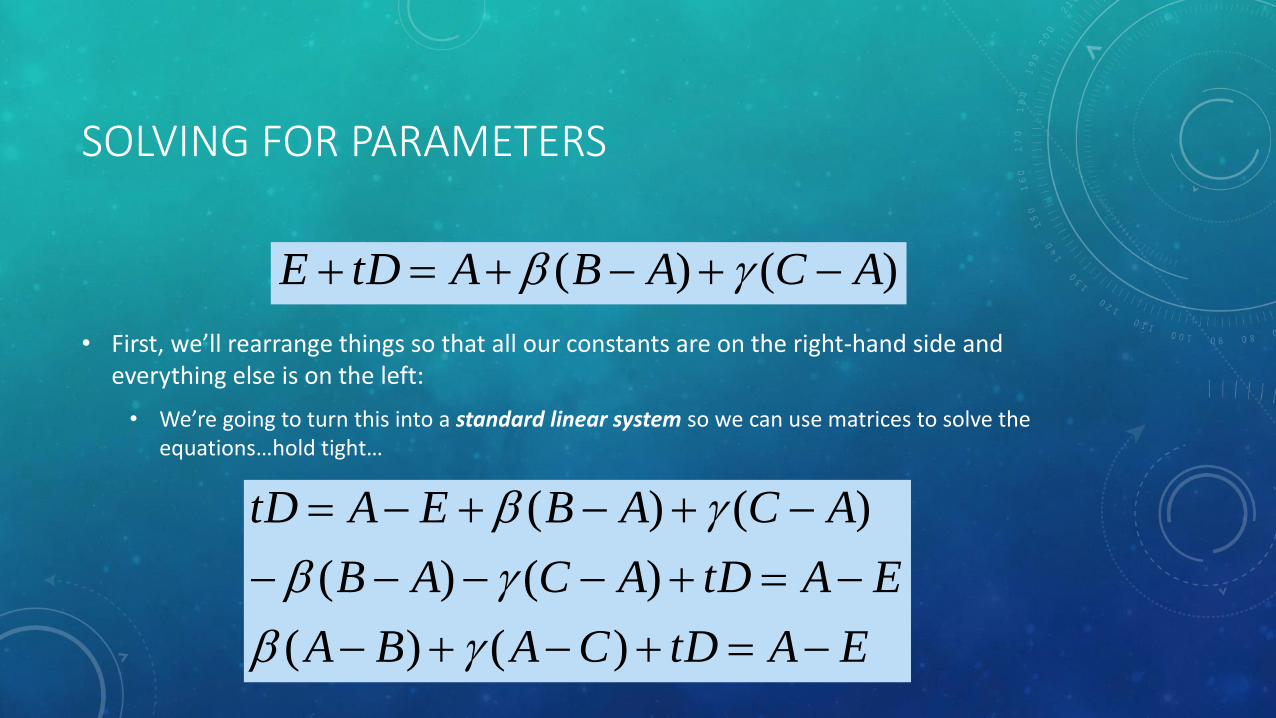
SOLVING FOR PARAMETERS
• First, we’ll rearrange things so that all our constants are on the right-hand side and everything else is on the left:
• We’re going to turn this into a standard linear system so we can use matrices to solve the equations…hold tight…
)()( ACABAtDE
EAtDCABA
EAtDACAB
ACABEAtD
)()(
)()(
)()(

SOLVING FOR PARAMETERS
• Then, we’ll expand this out into the individual coordinates:
• Remember: the (x,y,z) coordinates are known values
EADCABA
EADCABA
EADCABA
zztzzzzz
yytyyyyy
xxtxxxxx
)()(
)()(
)()(
EAtDCABA )()(

SOLVING FOR PARAMETERS
• Finally, we’ll turn this into a standard linear system of the form
EA
EA
EA
DCABA
DCABA
DCABA
zz
yy
xx
tzzzzz
yyyyy
xxxxx
NMV
EADCABA
EADCABA
EADCABA
zztzzzzz
yytyyyyy
xxtxxxxx
)()(
)()(
)()(

QUICK REVIEW: MATRIX MULTIPLICATION
• Matrix = effectively, a 2D array of numbers
• M = 3x3 matrix
• Vector = basically a matrix with one of the dimensions equaling 1
• V and N = 3x1 matrices = 3D column vectors
• When multiplying a matrix M by a vector V (IN THAT ORDER):
• Result = vector N with:
• Same # of rows as M
• Same # of columns as V
• For each value nR in N:
• Dot product of (Rth row of M) and (1st column of V)
2
1
0
2
1
0
222120
121110
020100
n
n
n
v
v
v
mmm
mmm
mmm
NMV
2221210202
2121110101
2021010000
vmvmvmn
vmvmvmn
vmvmvmn

BACK TO OUR LINEAR SYSTEM…
• So, for example, if I wanted the first equation back…
EA
EA
EA
DCABA
DCABA
DCABA
zz
yy
xx
tzzzzz
yyyyy
xxxxx
EADCABA xxtxxxxx )()(
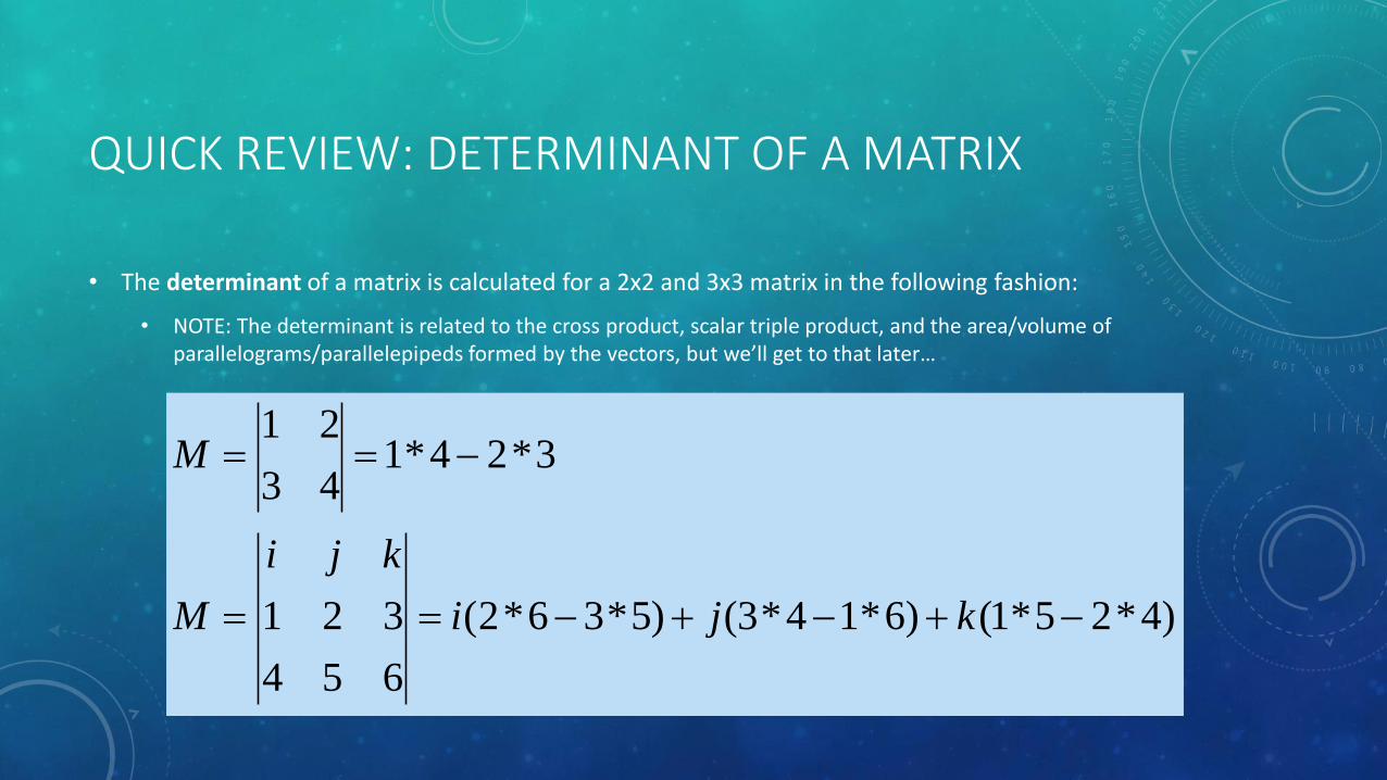
QUICK REVIEW: DETERMINANT OF A MATRIX
• The determinant of a matrix is calculated for a 2x2 and 3x3 matrix in the following fashion:
• NOTE: The determinant is related to the cross product, scalar triple product, and the area/volume of parallelograms/parallelepipeds formed by the vectors, but we’ll get to that later…
)4*25*1()6*14*3()5*36*2(
654
321
3*24*143
21
kji
kji
M
M

CRAMER’S RULE
• For 3x3 systems, a fast way to solve them is with Cramer’s Rule:
• Again, we’ll talk about how and why this works later…
• Given a system:
• For each coordinate of V (vi):
• Replace the ith column of matrix M with N
• Get the determinant
• Divide by the determinant of the original matrix M
• WARNING: If |M| = 0 no unique solution!
• May be no solution…may be INFINITE solutions…
NMV

APPLYING CRAMER’S RULE
• So, in determinant form, to solve for our parameters:
M
zzzzzz
yyyyyy
xxxxxx
tM
zzzzz
yyyyy
xxxxx
M
zzzzz
yyyyy
xxxxx
EACABA
EACABA
EACABA
DEABA
DEABA
DEABA
DCAEA
DCAEA
DCAEA
DCABA
DCABA
DCABA
zzzzz
yyyyy
xxxxx
M

APPLYING CRAMER’S RULE
• If we use dummy variables:
• We can show exactly what we need to calculate (and we can reduce the number of operations by calculating things like (ei – hf) once):
l
k
j
tifc
heb
gda
)()()()()()(
)()()()()()(
egdhcdigfbhfeiapp
kcbldaljcejbakft
p
kcblgaljchjbaki
p
egdhldigfkhfeij

CODING THE FUNCTION
• When coding the intersection function, we would want to terminate early if we can
• More efficient
• Let’s assume t has to be in the interval [t0 , t1]
• SO, our algorithm might look like:
• Compute t
• If (t < t0) OR (t > t1) return false
• Compute γ
• if (γ < 0) OR (γ > 1) return false
• Compute β
• If (β < 0) OR (β > 1 – γ) return false
• Return true

RAY-POLYGON INTERSECTION

WHAT IS A POLYGON, EXACTLY?• The official definition varies, but at bare minimum:
• Polygon = a figure with 3 or more vertices connected in sequence by straight-line segments (edges or sides of the polygon)
• Most loose definition any closed-polyline boundary
• More finicky definitions contained in single plane, edges have no common points other than their endpoints, no three successive points collinear
• Standard polygon or simple polygon = closed-polyline with no crossing edges

DOES A POLYGON LIE IN A SINGLE PLANE?
• In computer graphics, polygon not always in same plane:
• Round-off error
• I.e., points originally in single plane, but, after transformation,the points may be slightly off
• Fitting to surface makes non-planar polygons
• E.g., if using quads, approximation may “bend” the quad in half
• Thus, we usually use triangles to avoid this problem

DEGENERATE POLYGONS• Degenerate polygons = often used to describe polygon with:
• 3 or more collinear vertices generates a line segment
• E.g., in extreme case, triangle with no area
• Repeated vertex positions generates shape with:
• Extraneous lines
• Overlapping edges
• Edges with length 0

INTERSECTING WITH THE PLANE OF THE POLYGON
• If ALL of the vertices P1 through Pm of a polygon lie in the same plane first get intersection with plane
• Point-normal form of plane (we’ll just use the first point):
• Plugging in our ray equation for P:
0)( 1 NPP
ND
NEPt
NPENDt
NtDNPE
NPtDE
)(
)()(
0)(
0)(
1
1
1
1

ARE WE INSIDE THE POLYGON?
• Once we have our intersection point P, the question is: are we inside the polygon?
• One trick:
• Project point P and polygon to the XY plane
• Shoot a ray out from P
• Usually easiest to use X axis
• Check what we cross with this ray
• Number of edges OR direction of edges
• Two common approaches for the last step:
• Odd-Even Rule
• Nonzero Winding-Number Rule

ODD-EVEN RULE
• Also called odd-parity or even-odd rule
• Draw ray starting from position P
• Count how many edges we cross
• ODD inside polygon
• EVEN outside polygon

ASIDE: OTHER USES OF ODD-EVEN RULE
• Can use to check other kinds of regions
• E.g., area between two concentric circles
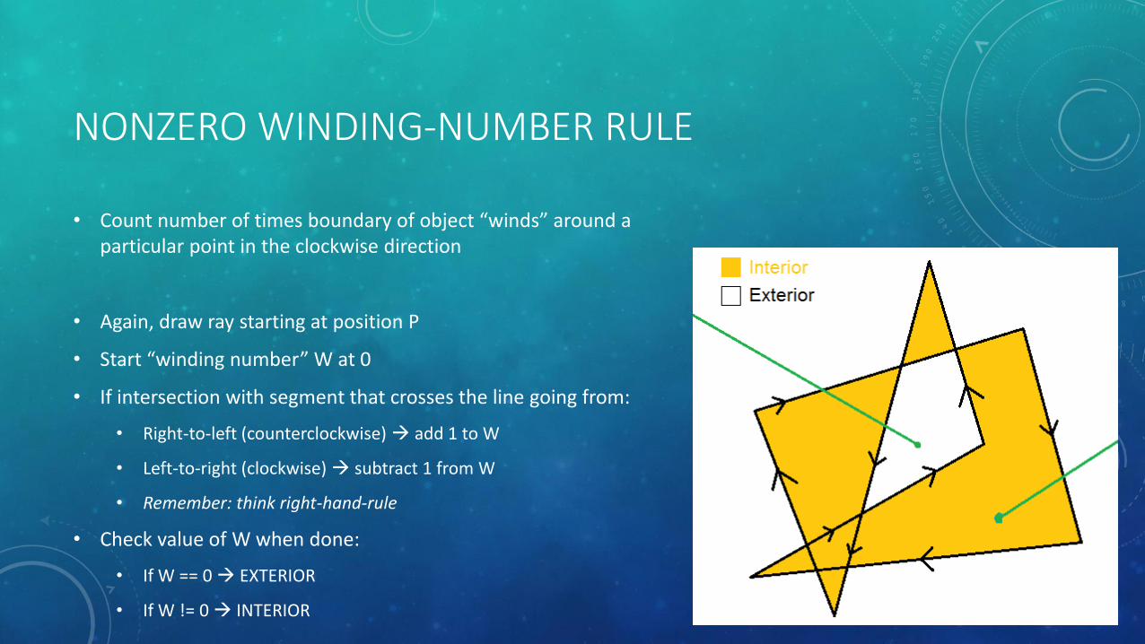
NONZERO WINDING-NUMBER RULE
• Count number of times boundary of object “winds” around a particular point in the clockwise direction
• Again, draw ray starting at position P
• Start “winding number” W at 0
• If intersection with segment that crosses the line going from:
• Right-to-left (counterclockwise) add 1 to W
• Left-to-right (clockwise) subtract 1 from W
• Remember: think right-hand-rule
• Check value of W when done:
• If W == 0 EXTERIOR
• If W != 0 INTERIOR

NONZERO WINDING-NUMBER RULE
• To check the direction of the edge relative to the line from P:
• Make vectors for each edge (in the correct winding order) vector Ei
• Make vector from P to distant point vector U
• Two options:
• Use cross product:
• If ( U x Ei ) = +Z axis right-to-left add 1 to winding number
• If ( U x Ei ) = –Z axis left-to-right subtract 1 from winding number
• Use dot product:
• Get vector V that is 1) perpendicular to U, and 2) goes right-to-left ( -uy , ux )
• If ( V · Ei ) > 0 right-to-left add 1 to winding number
• Otherwise left-to-right subtract 1 from winding number

ODD-EVEN VS. NONZERO WINDING-NUMBER• For simple objects (polygons that don’t self-intersect, circles, etc.), both approaches give same result
• However, more complex objects may give different results
• Usually, nonzero winding-number rule classifies some regions as interior that odd-even says are exterior
Odd-Even Rule Nonzero Winding-Number Rule

INSIDE-OUTSIDE PROBLEM
• Caveat: need to check we don’t cross endpoints (vertices)
• Otherwise, ambiguous we’ll talk in more detail how to deal with this when we get to filling polygons later…

ASIDE: CURVED PATHS?
• For curved paths, need to computer intersection points with underlying mathematical curve
• For nonzero winding-number also have to get tangent vectors
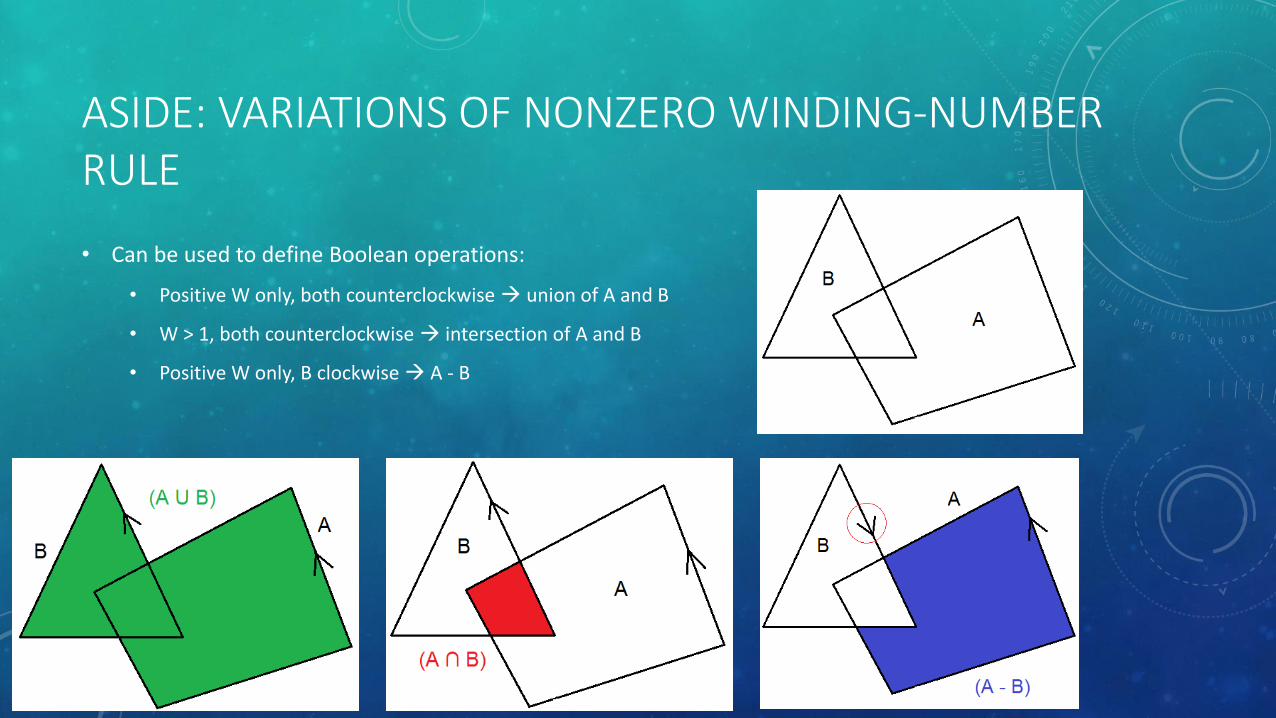
ASIDE: VARIATIONS OF NONZERO WINDING-NUMBER RULE
• Can be used to define Boolean operations:
• Positive W only, both counterclockwise union of A and B
• W > 1, both counterclockwise intersection of A and B
• Positive W only, B clockwise A - B

PROJECTING THE POLYGON PROBLEMS
• What if the projection of the polygon into XY is a LINE?
• E.g., the polygon is in the XZ plane?
• Solution: choose best among XY, YZ, or ZX planes
plane YZ use
plane ZXuse))()((
plane XY use))()(&(&))()((
else
xabsyabselseif
yabszabsxabszabsif
nn
nnnn

SHADING

SHADING MODEL
• Let’s assume we’ve:
• Intersected our view ray with every object in the scene
• Found the nearest intersection point (and associated object)
• The pixel value is computed by evaluating a shading model
• Shading model (or lighting model)
• Used to calculate the color of an illuminated position on the surface of an object
• In the slides that follow, we will concentrate on shading models that use point lights

POINT LIGHTS
• Point light
• Located at a single point in space
• Emit light in all directions

DIFFUSE REFLECTION
• Diffuse reflection = when white light hits an object, what we see as the “color” of an object
• Example: apple absorbs all frequencies except red has red diffuse color
• Underlying physics: surfaces with microfacets (bumpy, grainy, matte) reflects light in lots of different directions
• Ideal diffuse reflectors or Lambertian reflectors
• Incident light scattered with equal intensity in ALL directions, INDEPENDENT of viewing angle
• Depends on angle between NORMAL and DIRECTION-to-LIGHT angle of incidence

LAMBERTIAN SHADING
• Lambertian shading model
• Simplest of all shading models
• Amount of light energy that hits a surface proportional to angle of surface to light
• View-independent the viewer’s position doesn’t matter
• If:
• N = NORMALIZED normal
• L = NORMALIZED vector from point on surface to light source
• Then dot product is proportional to angle between L and N:
cosLN

LAMBERTIAN SHADING
• If the light is BEHIND the surface angle between L and N > 90 degrees dot product will be NEGATIVE
• So, we only want the max of 0 and the dot product:
• That said, our pixel color will be:
• …where:
• N = NORMALIZED normal
• L = NORMALIZED vector from point on surface to light source
• Subtract intersection point P from light position then normalize vector
• I = intensity of light
• kd = diffuse coefficient / diffuse color of surface
),0(max color Pixel LNIkd
),0(max LN

LAMBERTIAN SHADING
• Keep in mind that we basically have THREE equations (one for red, one for green, and one for blue)
• E.g., for the red pixel color have a red light intensity and a red diffuse coefficient
• N and L are the same in all cases
),0(max color Pixel LNIkd
PROBLEM WITH LAMBERTIAN SHADING
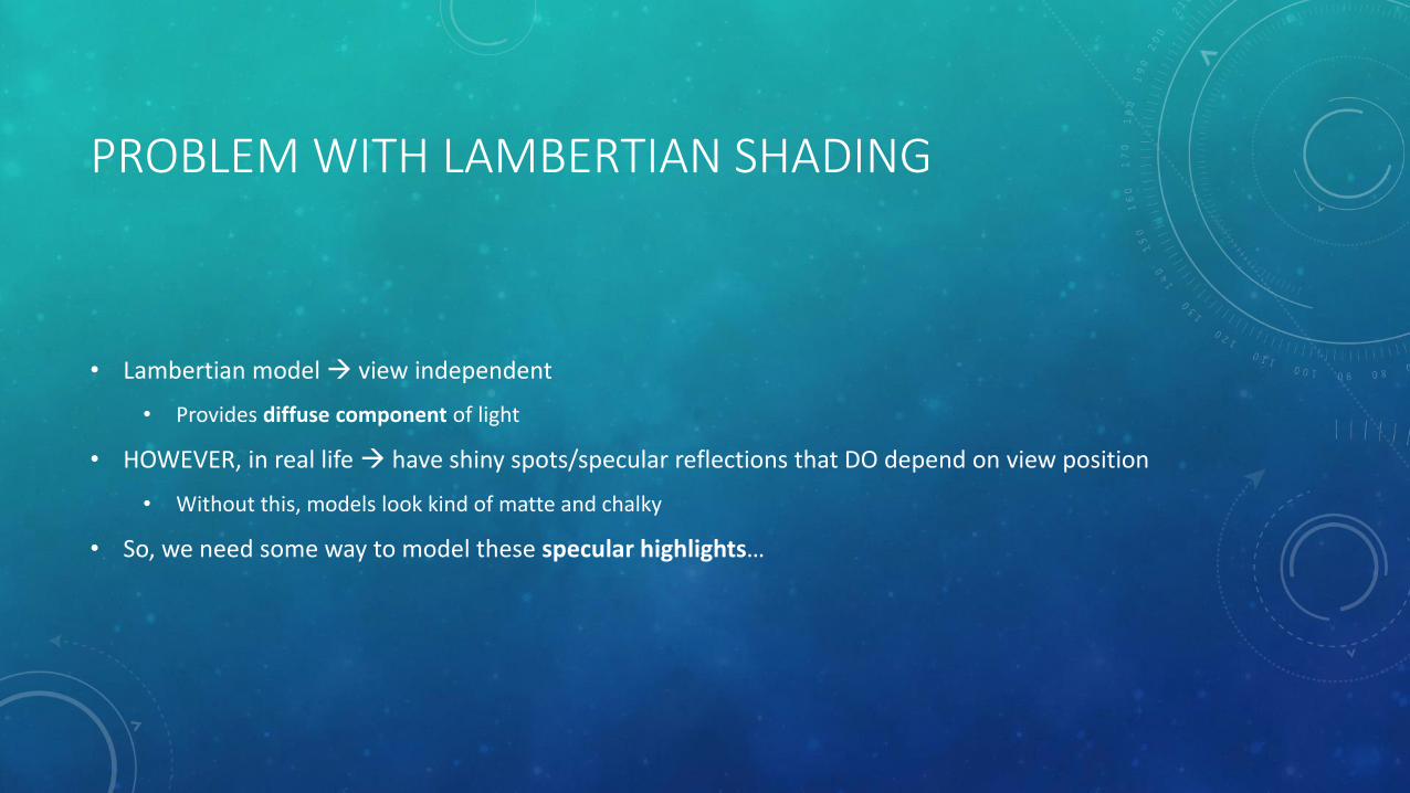
• Lambertian model view independent
• Provides diffuse component of light
• HOWEVER, in real life have shiny spots/specular reflections that DO depend on view position
• Without this, models look kind of matte and chalky
• So, we need some way to model these specular highlights…

BLINN-PHONG SHADING
• Blinn-Phong shading model
• Given:
• V = view direction NORMALIZED vector from intersection point to eye point
• Produce brightest reflection of light when V and L are symmetric about normal N
• Specular reflection = when all (or almost all) of the incident light is reflected back
• A shiny or reflective spot

BLINN-PHONG SHADING
• First, compute half-vector H
• Bisector of angle between V and L
• Both V and L are the same length can just add together to get average direction vector, then normalize!
• If perfect reflection H will be perfectly in line with normal N
• So, we want to look at:
LV
LVH
),0max( HN

BLINN-PHONG SHADING: ISSUES WITH THE HALF-VECTOR
• Problem: if V, L, and N are not coplanar slightly off
• Another problem: need to check if V and L are on same side of N (L · V > L · N) if so, don’t use specular effect at all

BLINN-PHONG SHADING: SHININESS
• Different surfaces reflect light over finite range of viewing positions
• Shiny surfaces narrow range
• Duller surfaces wider range
• So, we take the dot product to a power to make it decrease faster use Phong exponent or shininess s:
sHN ),0max(

BLINN-PHONG SHADING: SHININESS
• Typical values of s:
• 10 “eggshell”
• 100 mildly shiny
• 1000 really glossy
• 10,000 nearly mirror-like
BLINN-PHONG SHADING
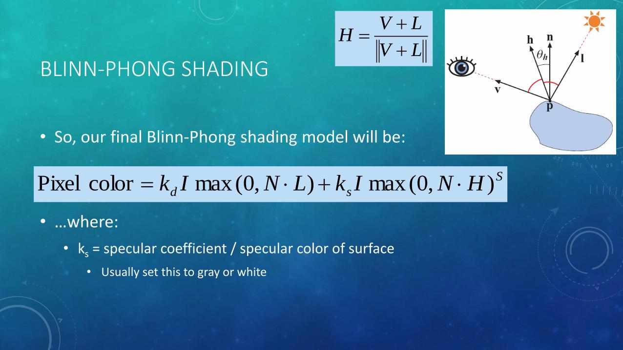
• So, our final Blinn-Phong shading model will be:
• …where:
• ks = specular coefficient / specular color of surface
• Usually set this to gray or white
S
sd HNIkLNIk ),0(max ),0(max color Pixel
LV
LVH

NORMALIZE YOUR VECTORS!!!
• IMPORTANT: DON’T FORGET TO NORMALIZE N, V, L, and H!!!
• Otherwise, we have lengths that we don’t want creeping into the dot products…

AMBIENT SHADING
• Using either of the two previous models, if the surface is facing away from the light completely black
• In real-life indirect reflections of other surfaces will cause SOME light to fall on those surfaces
• HORRIBLE HACK: Add a little bit of light to ALL surfaces ambient shading

AMBIENT SHADING
• Ambient shading
• Light all surfaces with “ambient” light that comes equally from everywhere
• Combined with Blinn-Phong, we get:
• …where
• Ia = ambient light intensity
• ka = surface’s ambient coefficient
• Can be kept separate to tune ambient light per surface OR can set the same as diffuse light coefficient
S
sdaa HNIkLNIkIk ),0(max ),0(max color Pixel

FINAL MODEL: DIFFUSE, SPECULAR, AND AMBIENT
S
sdaa HNIkLNIkIk ),0(max ),0(max color Pixel

MULTIPLE LIGHTS
• Light has the property of superposition
• I.e., effect caused by more than one light source = sum of effects from individual light sources
• So, to deal with multiple light sources, just sum all values up for diffuse and specular components (ambient light is only added once, however):
n
i
s
isidiaa HNkLNkIIk1
),0max(),0max(color Pixel

PROGRAMMING A RAY TRACER

BASIC ALGORITHM
• For the ray-tracer, the basic algorithm is as follows:
• For each pixel
• Compute viewing ray
• If (ray hits an object with t >= 0)
• Compute N
• Evaluate shading model and set pixel to that color
• Else
• Set pixel color to background color

OBJECT-ORIENTED APPROACH
• As we’ve seen, there are a lot of different kinds of objects you could intersect with:
• Spheres, triangles, planes, polygons, etc.
• Good OOP-based approach:
• Make generic class Surface
• Give Surface two functions:
• “hit()” returns whether a given ray hit the object
• Also hands back some kind of “hit-record” (intersection point, normal, etc.)
• “bounding-box()” returns max extends of surface
• Useful for optimization
• Have all other objects inherit from Surface and implement those two functions
• Then, you can just loop through one list of Surface instances
• Instead of separately going through your spheres, then your triangles, then…

MATERIALS
• A Material class is a good idea as well
• Have list of Materials that all objects share
• Store a pointer in Surface class to appropriate Material

SHADOWS AND REFLECTIONS

ADVANTAGES OF RAY TRACERS
• One really neat thing about ray tracers can add two additional effects very easily:
• Shadows
• Ideal Specular Reflections
• These are generally more difficult with object-order rendering
SHADOWS
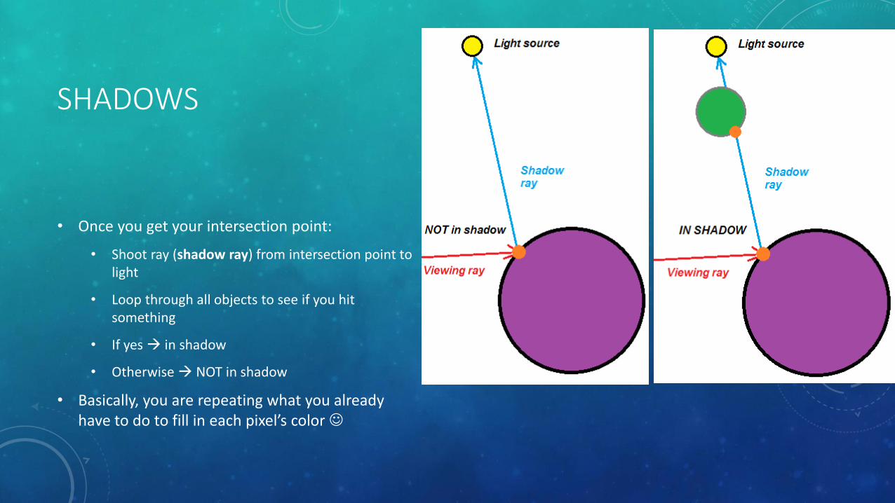
• Once you get your intersection point:
• Shoot ray (shadow ray) from intersection point to light
• Loop through all objects to see if you hit something
• If yes in shadow
• Otherwise NOT in shadow
• Basically, you are repeating what you already have to do to fill in each pixel’s color

SHADOWS
• Two things to note:
• 1) You should add ambient light to the output pixel color, irrespective of whether the point is in shadow
• 2) When shooting shadow ray usually start with t > e (where e is some tiny value)
• Start at 0 might intersect with THE SAME SURFACE you’re already on! (round-off error)

IDEAL SPECULAR REFLECTIONS
• In the same way, ideal specular reflections (or mirror reflections) are straightforward to add:
• Compute reflection vector R:
• Project D onto N subtract twice that vector to get R
• Check to see what object you hit with R and compute shading for that object assume it’s a function called “raycolor”
• Use raycolor as part of output color:
• …where km = “mirror reflection” coefficient, since some surfaces will reflect some colors better than others
• E.g., gold reflect yellow best
NNDDR )(2
)(c sRPraycolorkccolor m

IDEAL SPECULAR REFLECTIONS
• Three things to watch out for:
• 1) Same issue with shadows (don’t start at t = 0)
• 2) Need to include some kind of stopping criteria otherwise, keep bouncing around forever
• E.g., limit number of times you can recursively call raycolor()
• 3) For efficiency don’t call raycolor() if km = 0
• Not going to reflect anything anyway