CSE P 573 Artificial Intelligence

Spring 2014

Ali Farhadi Problem Spaces and Search

slides from Dan Klein, Stuart Russell, Andrew Moore, Dan Weld, Pieter Abbeel, Luke Zettelmoyer

Outline §  Agents that Plan Ahead

§  Search Problems

§  Uninformed Search Methods (part review for some) §  Depth-First Search §  Breadth-First Search §  Uniform-Cost Search

§  Heuristic Search Methods (new for all) §  Best First / Greedy Search

Review: Agents

Search -- the environment is: fully observable, single agent, deterministic, static, discrete

Agent

Sensors

?

Actuators

Environm

ent

Percepts

Actions

An  agent:  •  Perceives  and  acts  •  Selects  ac2ons  that  maximize  

its  u2lity  func2on  •  Has  a  goal    Environment:  •  Input  and  output  to  the  agent    

Reflex Agents

§  Reflex agents: §  Choose action based

on current percept (and maybe memory)

§  Do not consider the future consequences of their actions

§  Act on how the world IS §  Can a reflex agent

achieve goals?

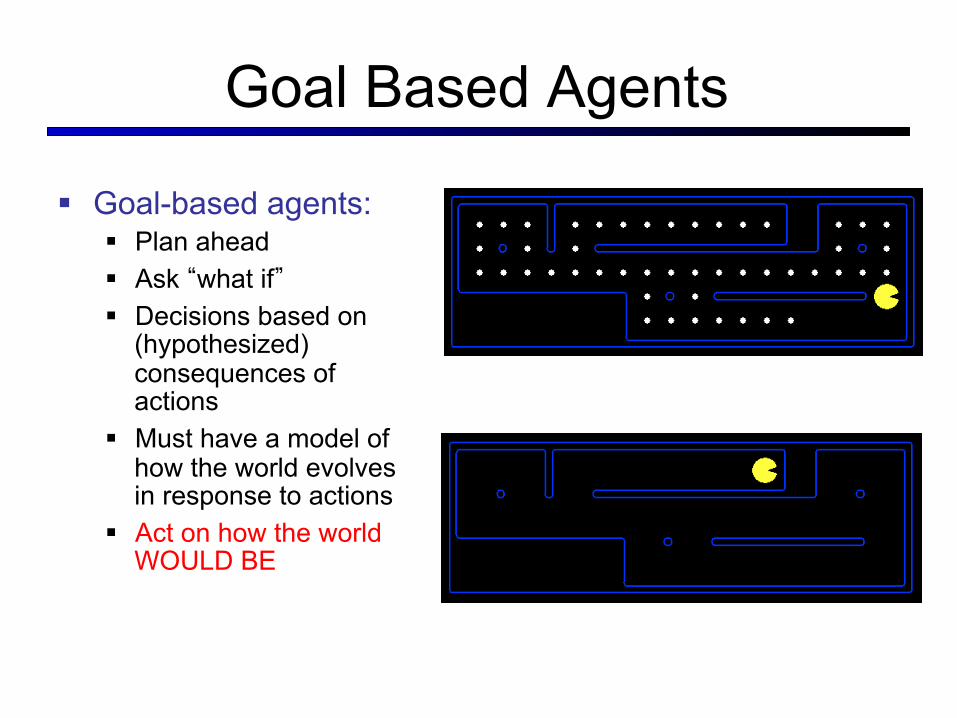
Goal Based Agents

§  Goal-based agents: §  Plan ahead §  Ask “what if” §  Decisions based on

(hypothesized) consequences of actions

§  Must have a model of how the world evolves in response to actions

§  Act on how the world WOULD BE

Search thru a

§  Set of states §  Successor Function [and costs - default to 1.0] §  Start state § Goal state [test]

• Path: start ⇒ a state satisfying goal test •  [May require shortest path] •  [Sometimes just need state passing test]

•  Input:

• Output:

Problem Space / State Space

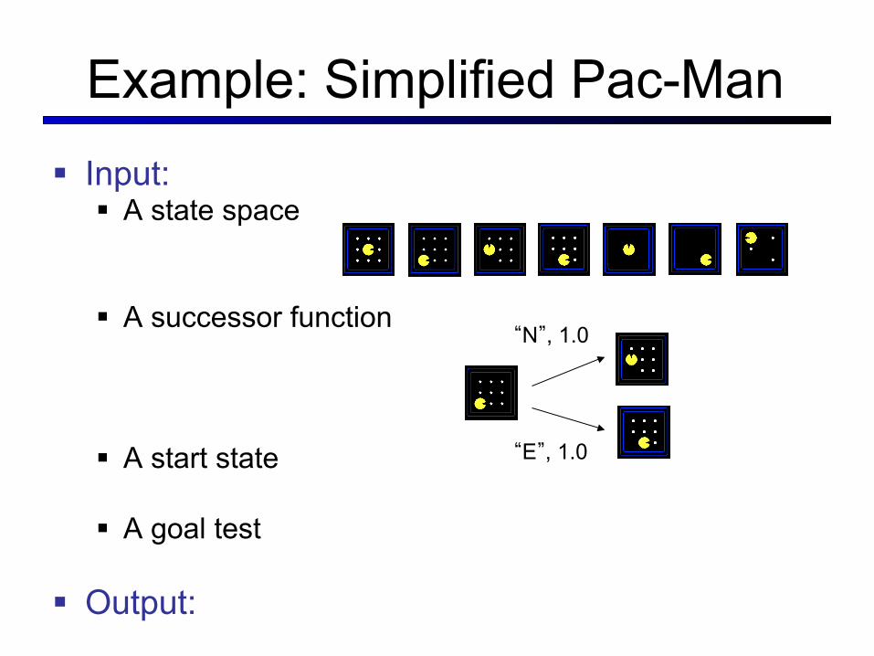
Example: Simplified Pac-Man §  Input:

§  A state space

§  A successor function

§  A start state

§  A goal test

§  Output:

“N”, 1.0

“E”, 1.0

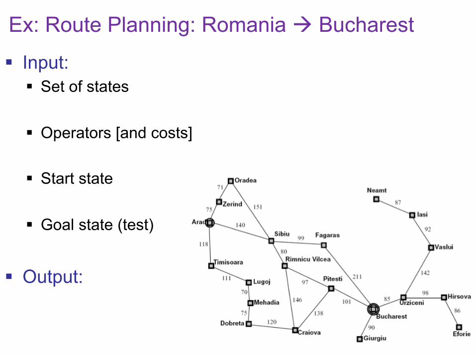
Ex: Route Planning: Romania à Bucharest

§  Input: §  Set of states

§  Operators [and costs]

§  Start state

§  Goal state (test)

§  Output:

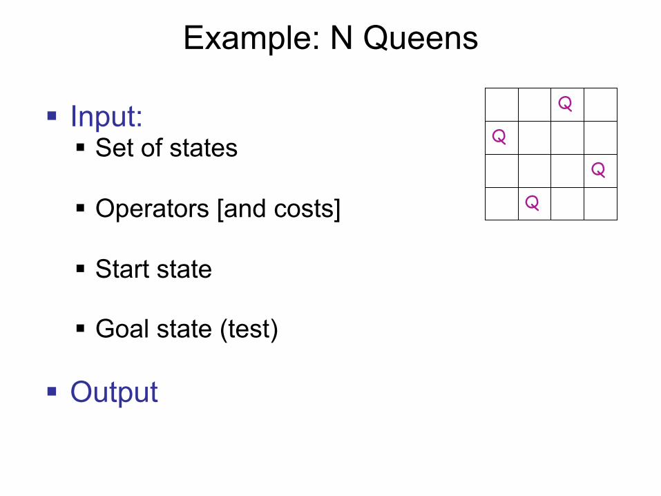
Example: N Queens

§  Input: §  Set of states

§ Operators [and costs]

§  Start state

§ Goal state (test)

§  Output

Q

Q

Q

Q

Algebraic Simplification

§  Input: §  Set of states

§  Operators [and costs]

§  Start state

§  Goal state (test)

§ Output:

What is in State Space?

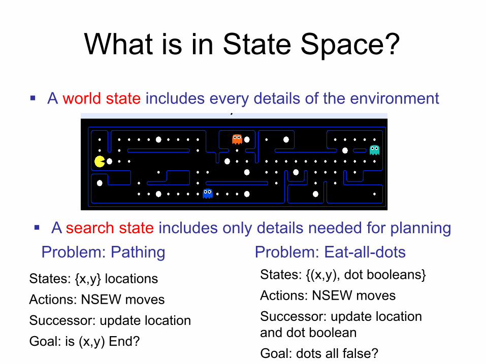
§  A world state includes every details of the environment

What’s#in#a#State#Space?#

!  Problem:#Pathing#!  States:#(x,y)#loca)on#!  Ac)ons:#NSEW#!  Successor:#update#loca)on#

only#!  Goal#test:#is#(x,y)=END#

!  Problem:#EatJAllJDots#!  States:#{(x,y),#dot#booleans}#!  Ac)ons:#NSEW#!  Successor:#update#loca)on#

and#possibly#a#dot#boolean#!  Goal#test:#dots#all#false#

The#world#state#includes#every#last#detail#of#the#environment#

A#search#state#keeps#only#the#details#needed#for#planning#(abstrac)on)#

§  A search state includes only details needed for planning Problem: Pathing Problem: Eat-all-dots

States: {x,y} locations Actions: NSEW moves Successor: update location Goal: is (x,y) End?

States: {(x,y), dot booleans} Actions: NSEW moves Successor: update location and dot boolean Goal: dots all false?

State Space Sizes?

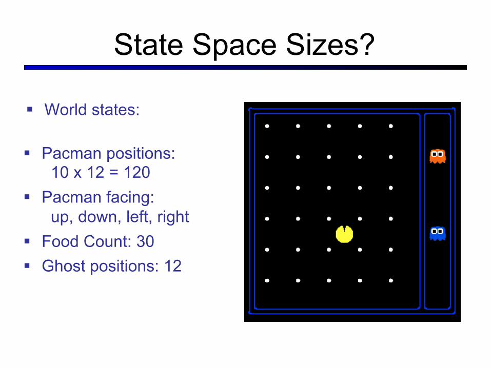
§  World states:

§  Pacman positions: 10 x 12 = 120

§  Pacman facing: up, down, left, right

§  Food Count: 30 §  Ghost positions: 12

State Space Sizes?

§  How many? §  World State:

§  States for Pathing:

§  States for eat-all-dots:

120*(230)*(122)*4

120

120*(230)

Quiz:#Safe#Passage#

!  Problem:#eat#all#dots#while#keeping#the#ghosts#permaJscared#!  What#does#the#state#space#have#to#specify?#

!  (agent#posi)on,#dot#booleans,#power#pellet#booleans,#remaining#scared#)me)#

State Space Graphs

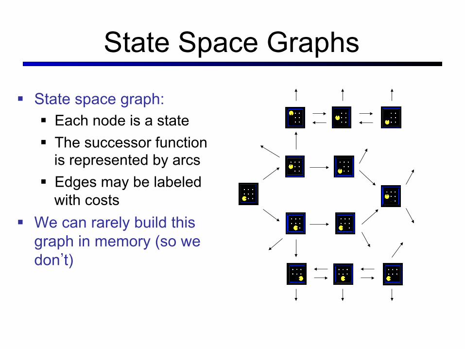
§  State space graph: §  Each node is a state §  The successor function

is represented by arcs §  Edges may be labeled

with costs §  We can rarely build this

graph in memory (so we don’t)

State#Space#Graphs#

!  State#space#graph:#A#mathema)cal#representa)on#of#a#search#problem#!  Nodes#are#(abstracted)#world#configura)ons#!  Arcs#represent#successors#(ac)on#results)#!  The#goal#test#is#a#set#of#goal#nodes#(maybe#only#one)#

!  In#a#search#graph,#each#state#occurs#only#once!#

!  We#can#rarely#build#this#full#graph#in#memory#(it’s#too#big),#but#it’s#a#useful#idea#

#

Search Trees

§  A search tree: §  Start state at the root node §  Children correspond to successors §  Nodes contain states, correspond to PLANS to those states §  Edges are labeled with actions and costs §  For most problems, we can never actually build the whole tree

“E”, 1.0 “N”, 1.0

Example: Tree Search

S

G

d

b

p q

c

e

h

a

f

r

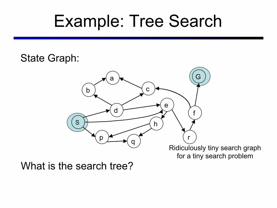
State Graph:

What is the search tree?

Ridiculously tiny search graph for a tiny search problem

State Graphs vs. Search Trees

S

a

b

d p

a

c

e

p

h

f

r

q

q c G

a

q e

p

h

f

r

q

q c G a

S

G

d

b

p q

c

e

h

a

f

r

We construct both on demand – and we construct as little as possible.

Each NODE in in the search tree is an entire PATH in the problem graph.

States vs. Nodes §  Nodes in state space graphs are problem states

§  Represent an abstracted state of the world §  Have successors, can be goal / non-goal, have multiple predecessors

§  Nodes in search trees are plans §  Represent a plan (sequence of actions) which results in the node’s

state §  Have a problem state and one parent, a path length, a depth & a cost §  The same problem state may be achieved by multiple search tree

nodes

Depth 5

Depth 6

Parent

Node

Search Nodes Problem States

Action

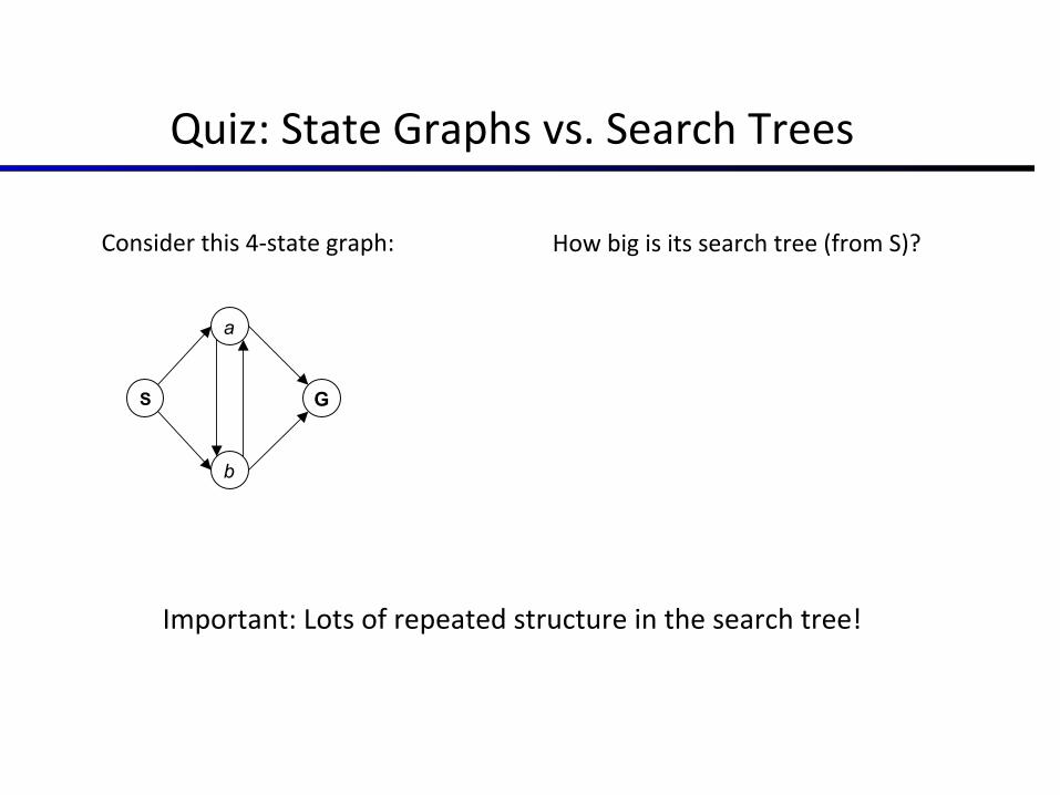
Quiz:#State#Graphs#vs.#Search#Trees#

S G

b

a

Consider#this#4Jstate#graph:##

Important:#Lots#of#repeated#structure#in#the#search#tree!#

How#big#is#its#search#tree#(from#S)?#

Building Search Trees

§  Search: §  Expand out possible plans § Maintain a fringe of unexpanded plans §  Try to expand as few tree nodes as possible

General Tree Search

§  Important ideas: §  Fringe §  Expansion §  Exploration strategy

§  Main question: which fringe nodes to explore?

Detailed pseudocode is in the book!

Search Methods §  Uninformed Search Methods (part review for some)

§  Depth-First Search §  Breadth-First Search §  Uniform-Cost Search

§  Heuristic Search Methods (new for all) §  Best First / Greedy Search

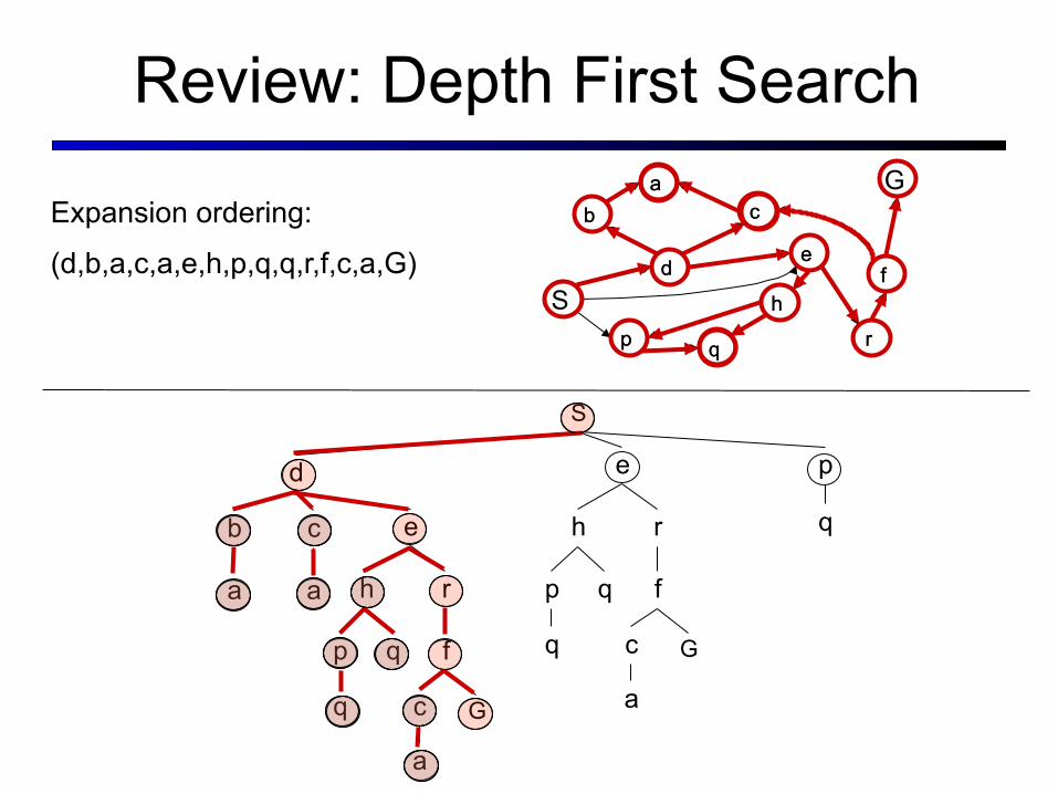
Review: Depth First Search

S

G

d

b

p q

c

e

h

a

f

r

Strategy: expand deepest node first

Implementation: Fringe is a LIFO queue (a stack)

Review: Depth First Search

S

a

b

d p

a

c

e

p

h

f

r

q

q c G

a

q e

p

h

f

r

q

q c G

a

S

G

d

b

p q

c

e

h

a

f

r q p

h f d

b a

c

e

r

Expansion ordering:

(d,b,a,c,a,e,h,p,q,q,r,f,c,a,G)

Review: Breadth First Search

S

G

d

b

p q

c

e

h

a

f

r

Strategy: expand shallowest node first Implementation: Fringe is a FIFO queue

Review: Breadth First Search

S

a

b

d p

a

c

e

p

h

f

r

q

q c G

a

q e

p

h

f

r

q

q c G

a

S

G

d

b

p q

c e

h

a

f

r

Search

Tiers

Expansion order: (S,d,e,p,b,c,e,h,r,q,a,a,h,r,p,q,f,p,q,f,q,c,G)

Search Algorithm Properties

§  Complete? Guaranteed to find a solution if one exists? §  Optimal? Guaranteed to find the least cost path? §  Time complexity? §  Space complexity?

Variables:

n Number of states in the problem b The maximum branching factor B

(the maximum number of successors for a state) C* Cost of least cost solution d Depth of the shallowest solution m Max depth of the search tree

DFS

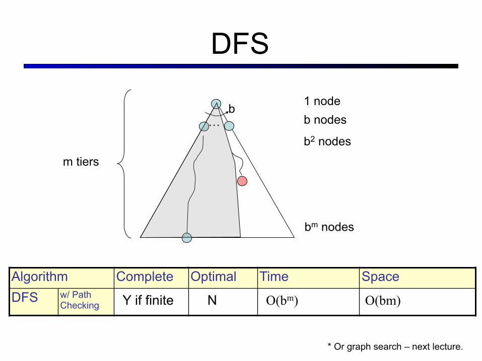
§  Infinite paths make DFS incomplete… §  How can we fix this? §  Check new nodes against path from S

§  Infinite search spaces still a problem §  If the left subtree has unbounded depth

Algorithm Complete Optimal Time Space DFS Depth First

Search N N O(BLMAX) O(LMAX)

START

GOAL a

b

No No Infinite Infinite

DFS

Algorithm Complete Optimal Time Space DFS w/ Path

Checking Y if finite N O(bm) O(bm)

…b 1 node

b nodes

b2 nodes

bm nodes

m tiers

* Or graph search – next lecture.

BFS

§  When is BFS optimal?

Algorithm Complete Optimal Time Space DFS w/ Path

Checking

BFS

Y N O(bm) O(bm)

Y Y* O(bd) O(bd)

…b 1 node

b nodes

b2 nodes

bm nodes

d tiers

bd nodes

Comparisons

§  When will BFS outperform DFS?

§  When will DFS outperform BFS?

34

Iterative Deepening Iterative deepening uses DFS as a subroutine:

1.  Do a DFS which only searches for paths of length 1 or less.

2.  If “1” failed, do a DFS which only searches paths of length 2 or less.

3.  If “2” failed, do a DFS which only searches paths of length 3 or less. ….and so on.

Algorithm Complete Optimal Time Space DFS w/ Path

Checking

BFS

ID

Y N O(bm) O(bm)

Y Y* O(bd) O(bd)

Y Y* O(bd) O(bd)

…b

Costs on Actions

Notice that BFS finds the shortest path in terms of number of transitions. It does not find the least-cost path.

START

GOAL

d

b

p q

c

e

h

a

f

r

2

9 2

8 1

8

2

3

1

4

4

15

1

3 2

2

Best-First Search §  Generalization of breadth-first search §  Priority queue of nodes to be explored §  Cost function f(n) applied to each node

Add initial state to priority queue While queue not empty Node = head(queue) If goal?(node) then return node

Add children of node to queue

Priority Queue Refresher

pq.push(key, value) inserts (key, value) into the queue.

pq.pop() returns the key with the lowest value, and removes it from the queue.

§  You can decrease a key’s priority by pushing it again

§  Unlike a regular queue, insertions aren’t constant time,

usually O(log n) §  We’ll need priority queues for cost-sensitive search methods

§  A priority queue is a data structure in which you can insert and retrieve (key, value) pairs with the following operations:

Uniform Cost Search

START

GOAL

d

b

p q

c

e

h

a

f

r

2

9 2

8 1

8

2

3

1

4

4

15

1

3 2

2

Expand cheapest node first: Fringe is a priority queue

Uniform Cost Search

S

a

b

d p

a

c

e

p

h

f

r

q

q c G

a

q e

p

h

f

r

q

q c G

a

Expansion order: (S,p,d,b,e,a,r,f,e,G) S

G

d

b

p q

c

e

h

a

f

r

3 9 1

16 4 11

5

7 13

8

10 11

17 11

0

6

3 9

1

1

2

8

8 1

15

1

2

Cost contours

2

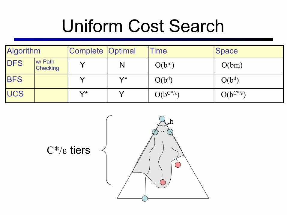
Uniform Cost Search Algorithm Complete Optimal Time Space DFS w/ Path

Checking

BFS

UCS

Y N O(bm) O(bm)

Y Y* O(bd) O(bd)

Y* Y O(bC*/ε) O(bC*/ε)

…b

C*/ε tiers

Uniform Cost Issues §  Remember: explores

increasing cost contours

§  The good: UCS is complete and optimal!

§  The bad: §  Explores options in every “direction”

§  No information about goal location Start Goal

…

c ≤ 3

c ≤ 2 c ≤ 1

Uniform Cost: Pac-Man

§  Cost of 1 for each action §  Explores all of the states, but one

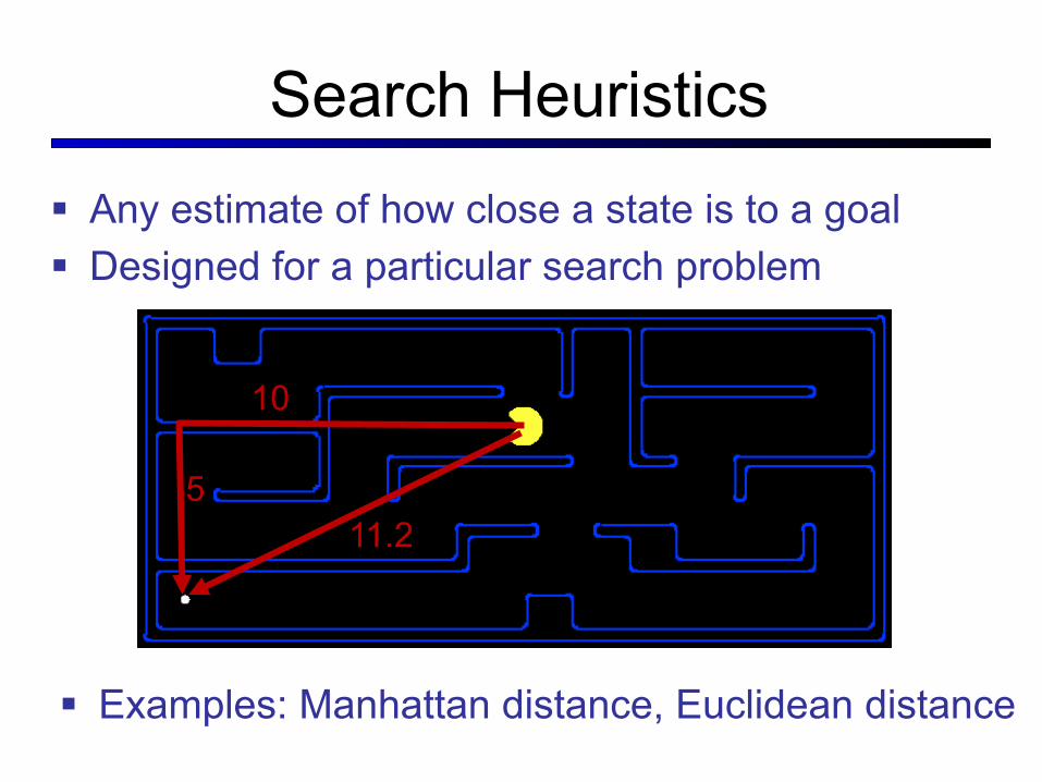
Search Heuristics

§  Any estimate of how close a state is to a goal §  Designed for a particular search problem

10

5 11.2

§  Examples: Manhattan distance, Euclidean distance

Heuristics

Best First / Greedy Search Best first with f(n) = heuristic estimate of distance to goal

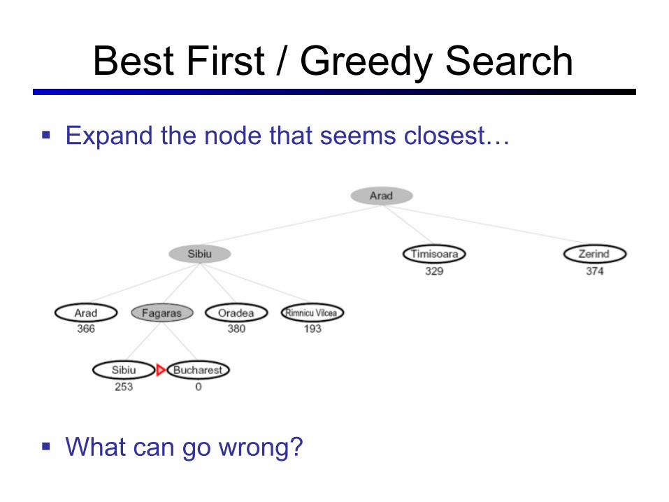
Best First / Greedy Search

§  Expand the node that seems closest…

§  What can go wrong?

Best First / Greedy Search §  A common case:

§  Best-first takes you straight to the (wrong) goal

§  Worst-case: like a badly-guided DFS in the worst case §  Can explore everything §  Can get stuck in loops if no

cycle checking

§  Like DFS in completeness (finite states w/ cycle checking)

…b

…b