Advanced Renewable Energy Technology

MJ2412

Concentrated Solar Power - Morocco Project

Authors:Mattia BerettaCamilo DiazHammad FarrukhSunay GuptaRachit KansalTimothy MuléCandace Shaw

Supervisors:Professor Andrew Martin

Lukas AichmayerRafael GuédezMonika TopelJorge Garrido

Monica Arnaudo

[1]

March 7, 2016

Abstract

In order to increase the share of renewables in the energymix ofMorocco, a newCSP power plant design proposalwas presented in this report, based on a program developed in MATLAB.

In total, six locations were considered for siting and after evaluating them using certain viability factors, Ouarza-zate was chosen as the most suitable location. Using the irradiation data from Solar Radiation Data (SODA) forOuarzazate in 2005, a central tower configuration was chosen after a performance evaluation against a parabolictrough configuration, using The United State’s National Renewable Energy Lab (NREL) System Advisor Model(SAM) software.

MATLAB was then used to dimension the solar field, thermal power at the receiver, the power cycle and the totalelectricity output, taking into account several factors and efficiencies.

Then, an optimization tool was developed in order to determine the ideal combination of storage size and turbinecapacity, considering both technical and economic performance. Transient operations were also modeled andevaluated and associated losses were included.

The final optimized plant produces 150 MW of power through a steam turbine, with seven hours of two-tank,molten salt storage. The plant annually produces 731 GWh of electricity, at an overall efficiency of 19.3%. Thepayback period period of the plant is 10 years, with a levelized cost of electricity of 16.7 ¢

kWh . The power plantalso ends up reducing annual carbon dioxide emissions by 403,500 tons.

Key Words: concentrated solar power, storage, solar tower, Morocco, Ouarzazate

1

Contents

List of Figures 3

List of Tables 3

1 Introduction 4

2 Selection Process 42.1 Location Selection . . . . . . . . . . . . . . . . . . . . . . . . . . . . . . . . . . . . . . . . . . . . . . . . . . . . . . 42.2 Technology Selection . . . . . . . . . . . . . . . . . . . . . . . . . . . . . . . . . . . . . . . . . . . . . . . . . . . . 6

3 Technical Analysis 73.1 Gathering Meteorological Data . . . . . . . . . . . . . . . . . . . . . . . . . . . . . . . . . . . . . . . . . . . . . . 7

3.1.1 Solar Field Design and Simulation . . . . . . . . . . . . . . . . . . . . . . . . . . . . . . . . . . . . . . . . 83.1.2 Solar Multiple . . . . . . . . . . . . . . . . . . . . . . . . . . . . . . . . . . . . . . . . . . . . . . . . . . . . 10

3.2 Calculating Power Output . . . . . . . . . . . . . . . . . . . . . . . . . . . . . . . . . . . . . . . . . . . . . . . . . 103.2.1 Choosing Thermal Storage or Hybridization . . . . . . . . . . . . . . . . . . . . . . . . . . . . . . . . . . 113.2.2 Optimization - Choosing the Right Combination of Turbines, Storage, and Hybridization . . . . . . . . 113.2.3 Justification of Hybridization . . . . . . . . . . . . . . . . . . . . . . . . . . . . . . . . . . . . . . . . . . . 13

3.3 Power Block . . . . . . . . . . . . . . . . . . . . . . . . . . . . . . . . . . . . . . . . . . . . . . . . . . . . . . . . . 133.3.1 Heat Exchanger (Steam Generator) . . . . . . . . . . . . . . . . . . . . . . . . . . . . . . . . . . . . . . . . 143.3.2 Turbines . . . . . . . . . . . . . . . . . . . . . . . . . . . . . . . . . . . . . . . . . . . . . . . . . . . . . . . 143.3.3 Condenser . . . . . . . . . . . . . . . . . . . . . . . . . . . . . . . . . . . . . . . . . . . . . . . . . . . . . . 143.3.4 Preheating . . . . . . . . . . . . . . . . . . . . . . . . . . . . . . . . . . . . . . . . . . . . . . . . . . . . . . 143.3.5 Feed Water Tank . . . . . . . . . . . . . . . . . . . . . . . . . . . . . . . . . . . . . . . . . . . . . . . . . . 143.3.6 Efficiency of the Power Cycle . . . . . . . . . . . . . . . . . . . . . . . . . . . . . . . . . . . . . . . . . . . 153.3.7 Operative Strategies . . . . . . . . . . . . . . . . . . . . . . . . . . . . . . . . . . . . . . . . . . . . . . . . 153.3.8 Transients Considered in the CSP Plant . . . . . . . . . . . . . . . . . . . . . . . . . . . . . . . . . . . . . 153.3.9 Daily Operation on a Typical Day . . . . . . . . . . . . . . . . . . . . . . . . . . . . . . . . . . . . . . . . . 16

3.3.9.1 Phase 1: Startup . . . . . . . . . . . . . . . . . . . . . . . . . . . . . . . . . . . . . . . . . . . . . 163.3.9.2 Phase 2: Full Operation . . . . . . . . . . . . . . . . . . . . . . . . . . . . . . . . . . . . . . . . . 173.3.9.3 Phase 3: Operation After Sunset . . . . . . . . . . . . . . . . . . . . . . . . . . . . . . . . . . . . 173.3.9.4 Shutdown . . . . . . . . . . . . . . . . . . . . . . . . . . . . . . . . . . . . . . . . . . . . . . . . . 183.3.9.5 Summary . . . . . . . . . . . . . . . . . . . . . . . . . . . . . . . . . . . . . . . . . . . . . . . . . 18

3.3.10 Limitations on Receiver . . . . . . . . . . . . . . . . . . . . . . . . . . . . . . . . . . . . . . . . . . . . . . 183.4 Transients . . . . . . . . . . . . . . . . . . . . . . . . . . . . . . . . . . . . . . . . . . . . . . . . . . . . . . . . . . 19

3.4.1 Impacts of Transients . . . . . . . . . . . . . . . . . . . . . . . . . . . . . . . . . . . . . . . . . . . . . . . . 193.4.2 Tower Receiver Temperature . . . . . . . . . . . . . . . . . . . . . . . . . . . . . . . . . . . . . . . . . . . 193.4.3 Operation of Plant . . . . . . . . . . . . . . . . . . . . . . . . . . . . . . . . . . . . . . . . . . . . . . . . . 213.4.4 Energy Needed for Molten Salt . . . . . . . . . . . . . . . . . . . . . . . . . . . . . . . . . . . . . . . . . . 223.4.5 Transients Energy Calculation for Turbine . . . . . . . . . . . . . . . . . . . . . . . . . . . . . . . . . . . . 22

4 The Algorithm Logic 244.1 Algorithm Assumptions . . . . . . . . . . . . . . . . . . . . . . . . . . . . . . . . . . . . . . . . . . . . . . . . . . 264.2 Results . . . . . . . . . . . . . . . . . . . . . . . . . . . . . . . . . . . . . . . . . . . . . . . . . . . . . . . . . . . . 26

5 Overall Performance of the Plant 29

6 Financial Analysis 306.1 Capital Expenditures (CAPEX) . . . . . . . . . . . . . . . . . . . . . . . . . . . . . . . . . . . . . . . . . . . . . . 306.2 Operational Expenditures (OPEX) . . . . . . . . . . . . . . . . . . . . . . . . . . . . . . . . . . . . . . . . . . . . 316.3 Tariffs . . . . . . . . . . . . . . . . . . . . . . . . . . . . . . . . . . . . . . . . . . . . . . . . . . . . . . . . . . . . . 33

7 Environmental Impacts 33

8 Conclusion 34

9 References 35

Appendices 39

2

List of Figures

1 Morocco GIS City Selection: Railways, Rivers, Electric Lines, & Lakes . . . . . . . . . . . . . . . . . 52 Morocco GIS City Selection: Roads . . . . . . . . . . . . . . . . . . . . . . . . . . . . . . . . . . . . . 53 Parabolic Trough . . . . . . . . . . . . . . . . . . . . . . . . . . . . . . . . . . . . . . . . . . . . . . . 64 Solar Tower . . . . . . . . . . . . . . . . . . . . . . . . . . . . . . . . . . . . . . . . . . . . . . . . . . 65 Block Diagram of Solar Field Design and Simulation . . . . . . . . . . . . . . . . . . . . . . . . . . . 106 Solar Multiples . . . . . . . . . . . . . . . . . . . . . . . . . . . . . . . . . . . . . . . . . . . . . . . . 107 Power Block Design . . . . . . . . . . . . . . . . . . . . . . . . . . . . . . . . . . . . . . . . . . . . . . 138 Receiver Temperature vs. Time . . . . . . . . . . . . . . . . . . . . . . . . . . . . . . . . . . . . . . . 219 Turbine Start-Up Curve . . . . . . . . . . . . . . . . . . . . . . . . . . . . . . . . . . . . . . . . . . . . 2210 Turbine Ramp Down Curve . . . . . . . . . . . . . . . . . . . . . . . . . . . . . . . . . . . . . . . . . 2311 Algorithm Logic . . . . . . . . . . . . . . . . . . . . . . . . . . . . . . . . . . . . . . . . . . . . . . . . 2512 Annual Revenue vs. Storage Size . . . . . . . . . . . . . . . . . . . . . . . . . . . . . . . . . . . . . . 2613 Annual Operating Costs vs. Storage Size . . . . . . . . . . . . . . . . . . . . . . . . . . . . . . . . . . 2714 Hybridization Amount vs. Storage Size . . . . . . . . . . . . . . . . . . . . . . . . . . . . . . . . . . 2715 Capital Costs vs. Storage Size . . . . . . . . . . . . . . . . . . . . . . . . . . . . . . . . . . . . . . . . 2816 Payback Period vs. Storage Size . . . . . . . . . . . . . . . . . . . . . . . . . . . . . . . . . . . . . . . 2817 Annual Heat Wasted vs. Storage Size . . . . . . . . . . . . . . . . . . . . . . . . . . . . . . . . . . . . 2918 CAPEX . . . . . . . . . . . . . . . . . . . . . . . . . . . . . . . . . . . . . . . . . . . . . . . . . . . . . 3119 OPEX . . . . . . . . . . . . . . . . . . . . . . . . . . . . . . . . . . . . . . . . . . . . . . . . . . . . . . 3120 Avoided Emissions . . . . . . . . . . . . . . . . . . . . . . . . . . . . . . . . . . . . . . . . . . . . . . 34

List of Tables

1 Location Selection . . . . . . . . . . . . . . . . . . . . . . . . . . . . . . . . . . . . . . . . . . . . . . . 52 Technology Selection from SAM . . . . . . . . . . . . . . . . . . . . . . . . . . . . . . . . . . . . . . . 73 Variable Definitions . . . . . . . . . . . . . . . . . . . . . . . . . . . . . . . . . . . . . . . . . . . . . . 84 Solar Field Loss Parameters . . . . . . . . . . . . . . . . . . . . . . . . . . . . . . . . . . . . . . . . . 95 Variable Definitions . . . . . . . . . . . . . . . . . . . . . . . . . . . . . . . . . . . . . . . . . . . . . . 96 Tariff Structure for CSP Plant . . . . . . . . . . . . . . . . . . . . . . . . . . . . . . . . . . . . . . . . 117 Tariff Scheme for Various Moroccan Cities . . . . . . . . . . . . . . . . . . . . . . . . . . . . . . . . . 128 Power Cycle Efficiencies . . . . . . . . . . . . . . . . . . . . . . . . . . . . . . . . . . . . . . . . . . . 159 Representative Day of Operation . . . . . . . . . . . . . . . . . . . . . . . . . . . . . . . . . . . . . . 1610 Variable Definitions . . . . . . . . . . . . . . . . . . . . . . . . . . . . . . . . . . . . . . . . . . . . . . 2011 Receiver Temperature vs Time . . . . . . . . . . . . . . . . . . . . . . . . . . . . . . . . . . . . . . . . 2012 Total CSP Plant Performance . . . . . . . . . . . . . . . . . . . . . . . . . . . . . . . . . . . . . . . . . 3013 Cost Factors . . . . . . . . . . . . . . . . . . . . . . . . . . . . . . . . . . . . . . . . . . . . . . . . . . 3014 CAPEX . . . . . . . . . . . . . . . . . . . . . . . . . . . . . . . . . . . . . . . . . . . . . . . . . . . . . 3115 OPEX . . . . . . . . . . . . . . . . . . . . . . . . . . . . . . . . . . . . . . . . . . . . . . . . . . . . . . 3216 Equipment List . . . . . . . . . . . . . . . . . . . . . . . . . . . . . . . . . . . . . . . . . . . . . . . . 3217 Variable Definitions . . . . . . . . . . . . . . . . . . . . . . . . . . . . . . . . . . . . . . . . . . . . . . 3318 Final Tariff Structure for CSP Plant . . . . . . . . . . . . . . . . . . . . . . . . . . . . . . . . . . . . . 33

3

1 Introduction

With growing global concern for the environment, as well as a strong desire to shift away from foreign energydependance, Morocco has recently been increasing its availability of concentrated solar power (CSP) electricityproduction. Morocco currently imports fossil fuels to satisfy 97% of its energy needs and the introduction ofnew CSP plants in the country has the potential to greatly help the western kingdom on a course for energyindependence, and to set off a movement of harnessing the vast solar resource throughout other countries inNorthern Africa [2].

Long termplans have taken into account the idea of transmitting the excess power generated fromCSP inMoroccothroughout Northern Africa and eventually into the European Union. With this potential source of renewablepower for Europe and figures from the International Energy Agency estimating that 11% of the world’s electricitycould come from CSP by 2050, organizations such as TheWorld Bank, The African Development Bank, The Euro-pean Investment Bank, as well as private investors are all getting involved with theWestern Kingdom’s ambitiousCSP plans [3].

Different possible locations aroundMorocco and various forms of CSP technologies can be suitable for the devel-opment of future plants. This report details a selection process that was undertaken to establish the best site andmechanism for a newCSP plant to be installed. A full financial and power generation investigationwas conductedas well and can be seen in detail in the following sections.

2 Selection Process

In order to move forward with a project for a new CSP plant in Morocco it was necessary to determine both theideal location in the country, as well as the preferred CSP technology. Various methods were used to eventuallydetermine that Ouarzazate, Moroccowas the best location for a newplant and that a tower configurationwould bethe best technology to implement. The details of the selection processes can be seen in the following subsections.

2.1 Location Selection

The location selection for the CSP plant was done considering the parameters shown in Table 1. Each parameterwas given a certain weightage on a 1 to 5 scale by the analyzing team, and that parameter was assessed for thelocation. Geographic Information Systems (GIS) as well as satellite imaging was used to determine the rankingsfor each of the criteria. ArcGIS software was utilized for analyzing areas of high solar irradiation, road, railwayand grid infrastructure locations, water resource locations, and distance to city centers. Figure 1 is a GIS mapcombining layers of datasets listed in Table 1, except for road infrastructure which had to be on a separate mapfor simplicity of reading which is shown in Figure 2.

4

Figure 1: Morocco GIS City Selection: Railways,Rivers, Electric Lines, & Lakes Figure 2: Morocco GIS City Selection: Roads

Solar irradiation was given the highest weightage considering the fact that it is the most important parameterfor a solar power plant because it is the primary resource for the plant. Access to water and grid accessibilitywere given a weightage of 4 as the second most important criteria because they involve large infrastructure costs.Road and railroad accessibility and distance to the consumption centers were weighted 3 and 1 respectively, thereason being the importance of the road and rail access to facilitate the construction and operation of the plant.The topography and the proximity to other CSP plants were considered to be least important because they haveminimal impact of the plant. The topography only affect the design process, but that impact is also small. Thetable below details the location selection process:

Criteria Weigh

tage

Sebkhat Tah

Ouarzazate

Ain B

eni M

athar

Foum

AlOuad

Boujd

our

Midelt

Solar Irradiation 5 3 4 2 3 3 3

Access to Water (Rivers, Lakes) 4 2 5 4 1 1 4

Grid Accessibility (from the map) 4 2 5 5 3 5 5

Road Accessibility (from the map) 3 2 4 5 3 5 5

Proximity to Existing CSP Plants 1 0 5 5 2 0 0

Distance to Consumption Centers 1 4 4 3 4 5 3

Topography (Flat or Mountainous) 1 4 4 3 4 5 3

Total - 43 87 77 48 53 77

Table 1: Location Selection

Based on the selection process in Table 1, Ouarzazate was decided to be the optimal location for a new CSP plant.

5

2.2 Technology Selection

Twomajor technologies were compared for use in the new CSP plant: central tower receiver and parabolic trough.Examples of each are shown in Figure 3 and 4 respectively.

Figure 3: Parabolic Trough [4] Figure 4: Solar Tower [5]

Both technologies have their share of advantages and disadvantages. In order to determine which technologywould result in the best plant layout a simulation software for the design of CSP plants was used. The UnitedState’s National Renewable Energy Lab (NREL) has a System Advisor Model (SAM) which was used as startingpoint for the project. General reference data was used as the input into SAM which included cost, material, effi-ciencies and other useful parameters for each technology. The simulation on SAMwas run aiming at a generationtarget of at least 110 megawatts of electricty (MWe) while in production. The results were evaluated on an eco-nomic basis, so the cheaper technology able to provide the desired output was chosen. The results are seen inTable 2, and it was apparent that tower technology was the optimal choice.

6

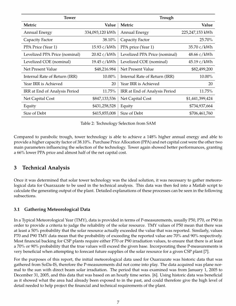
Tower Trough

Metric Value Metric Value

Annual Energy 334,093,120 kWh Annual Energy 225,247,153 kWh

Capacity Factor 38.10% Capacity Factor 25.70%

PPA Price (Year 1) 15.93 ¢/kWh PPA price (Year 1) 35.70 ¢/kWh

Levelized PPA Price (nominal) 20.82 ¢/kWh Levelized PPA Price (nominal) 48.66 ¢/kWh

Levelized COE (nominal) 19.45 ¢/kWh Levelized COE (nominal) 45.19 ¢/kWh

Net Present Value $48,216.984 Net Present Value $82,499,200

Internal Rate of Return (IRR) 10.00% Internal Rate of Return (IRR) 10.00%

Year IRR is Achieved 20 Year IRR is Achieved 20

IRR at End of Analysis Period 11.75% IRR at End of Analysis Period 11.75%

Net Capital Cost $847,133,536 Net Capital Cost $1,441,399,424

Equity $431,258,528 Equity $734,937,664

Size of Debt $415,855,008 Size of Debt $706,461,760

Table 2: Technology Selection from SAM

Compared to parabolic trough, tower technology is able to achieve a 148% higher annual energy and able toprovide a higher capacity factor of 38.10%. Purchase Price Allocation (PPA) and net capital cost were the other twomain parameters influencing the selection of the technology. Tower again showed better performances, grantinga 66% lower PPA price and almost half of the net capital cost.

3 Technical Analysis

Once it was determined that solar tower technology was the ideal solution, it was necessary to gather meteoro-logical data for Ouarzazate to be used in the technical analysis. This data was then fed into a Matlab script tocalculate the generating output of the plant. Detailed explanations of these processes can be seen in the followingsubsections.

3.1 Gathering Meteorological Data

In a Typical Meteorological Year (TMY), data is provided in terms of P-measurements, usually P50, P70, or P90 inorder to provide a criteria to judge the reliability of the solar resource. TMY values of P50 mean that there wasat least a 50% probability that the solar resource actually exceeded the value that was reported. Similarly, valuesP70 and P90 TMY data mean that the probability of exceeding the reported value are 70% and 90% respectively.Most financial backing for CSP plants require either P70 or P90 irradiation values, to ensure that there is at leasta 70% or 90% probability that the true values will exceed the given base. Incorporating these P-measurements isvery beneficial when attempting to forecast future supplies of the solar resource for a given CSP plant [7].

For the purposes of this report, the initial meteorological data used for Ouarzazate was historic data that wasgathered from SoDa-IS, therefore the P-measurements did not come into play. The data acquired was plane nor-mal to the sun with direct beam solar irradiation. The period that was examined was from January 1, 2005 toDecember 31, 2005, and this data that was based on an hourly time series. [6]. Using historic data was beneficialas it showed what the area had already been exposed to in the past, and could therefore give the high level ofdetail needed to help project the financial and technical requirements of the plant.

7

3.1.1 Solar Field Design and Simulation

The total land available for the project was set to 579 hectares, or 5,790,000m2. Of this total 904,355m2 was thesuggested mirror area. Part of the total available land had to set aside to account for the land requirements of thetower receiver, storage system, and power block; which was calculated to be 4,531.7m2. The first ring of mirrorswas then placed 38meters from the center point of the field. The solar field designwasmade using aMatlab scriptwhich was able to divide the available land into different cells. The script could then evaluate the performance ofeach cell in the field.

The field was set to have a circular shape and was divided in 12 equidistant radial and azimuthal regions. Thisdivision of the field resulted in a total of 144 cells in the field. This was considered adequate as it helped reducedthe computational time required to describe the solar field, but was still able to provide accurate results of howthe field operated.

Each cell was assigned with a characteristic heliostat density, which decreased as the distance from the solar re-ceiver grew larger. This was becausemirrors located in the outer rings have lower performance compared to thoselocated in the inner rings, so it was not beneficial to have a very high mirror density in the outskirts of the field.

A known expression for calculating the heliostat density in a solar tower configuration can be seen below [16]:

ρF = 0.721 ∗ exp(−0.29rHhT

) + 0.03

Where:

Variable Description Units

ρF Heliostat Density m2helio

m2land

rH Radial Position of the Heliostat m

hT Height of the Tower m

Table 3: Variable Definitions

However, when using this formula the total mirror area of the field was considerably lower than the referencevalue that was mentioned in the project description for this CSP plant design. In order to determine a heliostatdensity that was comparable with the reference plant, a Matlab code was developed to iterate through differentdensities for each circular ring in the field. A line of best fit was developed for the initial part of the exponentialfunction of the given formula, and the iterations in Matlab were executed by applying the slope of this line. Theresults were adjusted to resemble the heliostat densities and field area of the given reference plant.

After dividing the solar field in cells, it was necessary to define the performance of a representative heliostat foreach cell. In order to accomplish this, a series of loss parameters such as surface& cosine effectiveness, shadowing,blocking, attenuation, and spillage factor were all taken into account. These factors are reported in Table 4

8

Variable Value

Surface Effectiveness 0.92 ∗ 0.966 = 0.88872 [17]

Shadowing Factor 0.05 [16]

Blockage Factor 0.05 [16]

Table 4: Solar Field Loss Parameters

The calculation of the attenuation factor was dependent on the distance of the heliostats from the central receiver.Due to this varying parameter the attenuation losses could not be given as an overall factor as the previous losses.Therefore, the estimation of the attenuation losses was done using the following formulas [19]:

AttenuationFactor = 0.99326 − 0.1046 ∗ S + 0.017 ∗ S2 − 0.002845 ∗ S3

S =√r2cell + (htower − hheliostat)2

Where:

Variable Description Units

r2cell Radial Distance of the Cell m

htower Height of the Solar Tower m

hheliostat Height of the Heliostat Pedestal m

S Minimum Distance of the Representing Heliostatfrom the Receiver Tower

m

Table 5: Variable Definitions

The heliostat height was assumed to be 6 meters, whereas the tower height was given in the project descriptionand it was equal to 163.2 meters [18, 17].

The next step in the design process was the importation of an excel file containing hourly incoming solar radiationfor each day of the year 2005 and all of the angles required to calculate the solar azimuth and zenith angles. Thesolar azimuth and zenith angles were then further used to define the vectors vs and vt. The vector vs describesthe solar position and vt is the vector between the mirror pivot and the center of the receiver. Using vs and vt, itwas possible to define nh, the normal vector to the pivot of the mirrors. nh multiplied by vt resulted in the cosineeffectiveness of the cell.

After calculating all of the data about the solar radiation and the relevant angles, it was possible to run the sim-ulation for the entire solar field during a year of operation. The net electrical power output of the plant for eachhour of the year was then calculated using the efficiencies of receiver, thermal cycle and the generator. In orderto optimize the storage system, a different type of output was created which was not the electrical output power,but the thermal power. This was done in order to work more easily with the thermal energy storage systems inthe plant. A block diagram showing the solar field design and simulation process can be seen in Figure 5.

9

Figure 5: Block Diagram of Solar Field Design and Simulation

3.1.2 Solar Multiple

The solar multiple of the plant was calculated to be 1.83 on summer solstice (21st June). In order to have a com-parative view of the plant around the year, solar multiple was also calculated for other days of the year as shownin Figure 6. The meteorological data revealed that there was a lack of solar irradiation on the winter solstice, mostlikely due to cloud cover. Because of this the solar multiple was calculated for 24th of December for comparison.

Figure 6: Solar Multiples

3.2 Calculating Power Output

Since the output of the CSP plant is dependent on the Sun, it means that it varies with the rise and fall of theSun through the day and the year. However, the minimum requirement from the grid is always 110 MW for allthe hours the plant is operating during. If the plant were to not employ any storage or hybridization and solely

10

rely on the field’s output, it would not be able to meet the requirement for 2,775 hours in a year, or the equivalentof 115 days. Hence, there is a clear need for either storage or hybridization to meet the grid requirement for theduration of plant operation.

3.2.1 Choosing Thermal Storage or Hybridization

There is now a choice between storage or hybridization. Storage in this case would entail a two-tank, molten ni-trate salt system with a cold tank at 290oC and a hot tank at 565oC. The storage would be daily, meaning that itwould retain heat for a maximum of 10-12 hours and would be sized accordingly. At times when the productionfrom the solar field far exceeds the requirements from the grid, the extra heat would be used to heat the salt. Then,at times when the production falls short, the same heat would be used to cover the supply shortfall and meet thedemand requirement.

The hybridization option involves burning natural gas for all the times the plant is not able to produce enoughelectricity to meet the minimum requirement. It does not involve utilizing the excess energy produced by thefield, in any way.

Given the above description, it should not be surprising that with just a hybridization option, 761.4 GWh of elec-tricity would be wasted in a year, an average of 2.09 GWh per day. With 6 hours of storage and the same turbinespecifications, 19.7 GWh of electricity could be saved, averaging 54 MWh per day.

Moreover, environmental stewardship was one of the main goals of the power plant design, which is why associ-ated carbon dioxide emissions were an important consideration in making the decision. Given howmuch energyis saved via storage, and how it is carbon-neutral in its operation, storage was chosen as the main driver for theplant. Hybridization was included as a back-up option, for very cloudy days or weeks, where neither the plantnor the storage would be enough.

3.2.2 Optimization - Choosing the Right Combination of Turbines, Storage, and Hybridization

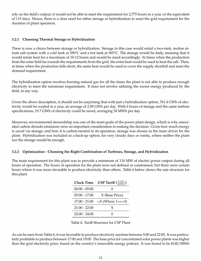
The main requirement for this plant was to provide a minimum of 110 MW of electric power output during allhours of operation. The hours of operation for the plant were not defined or constrained, but there were certainhours where it was more favorable to produce electricity than others. Table 6 below shows the rate structure forthis plant.

Clock Time CSP Tariff ( USDMWh )

00:00 - 05:00 0

05:00 - 17:00 X (Base Price)

17:00 - 21:00 αX (Where 1<α<3)

21:00 - 22:00 X

22:00 - 24:00 0

Table 6: Tariff Structure for CSP Plant

As can be seen from Table 6, it was favorable to produce electricity anytime between 5:00 and 22:00. It was particu-larly profitable to produce between 17:00 and 19:00. The base price for concentrated solar power plants was higherthan the grid electricity price, based on the country’s renewable energy policies. It was found to be $140/MWh

11

of electricity [23].

To find α, the multiplier for the time period of 17:00 to 21:00, current Moroccan time-of-use grid policies wereexamined. While no policies were found for the city of Ouarzazate, policies were found for various Moroccancities, including its capital Rabat as seen in Table 7.

Region Ratio of Mid-Peak/Off-Peak Ratio of Peak/ Off-Peak

Casablanca 1.532 1.521

Rabat 1.526 1.517

Tanger 1.437 1.452

Table 7: Tariff Scheme for Various Moroccan Cities [24]

Here, off-peak hours range from 22:00 to 7:00, mid-peak hours range from 7:00 to 17:00 and peak hours rangefrom 17:00 to 22:00. From Table 6, it can be seen that the multiplier α ranges from 17:00 to 21:00 and is a multipleof the base price, which ranges from 5:00 to 17:00. From the above information, it was clear that the ratio neededto calculate α was the ratio of peak power to mid-peak power. The average of the ratios from the three cities wastaken and was found to be 1.497.

Since the only constraint was to produce a minimum of 110 MW and the main objective was to maximize revenueand minimize payback period, the turbine capacity and the size of the storage were both taken as variables. Tocarry out the optimization, a range of possible values for both variables needed to be created, which would thenbe iterated to give the best possible result.

For determining the possible turbine capacities, different turbine manufacturers were considered. Siemens, aworldwide leading turbine manufacturer, was finally chosen to ensure the highest quality for the price paid. Themajor Siemens turbines that were examined were the SST-600 series of 150 MW capacity, the SST-700 series of 175MW capacity, and SST-900 series of 250 MW capacity [25, 26, 27]. Hence, 150, 175 and 250 MW formed the rangeof possible turbine sizes.

From the tariff scheme in Table 6, it was determined that the size of the thermal storage could range between 1to 10 hours. This was aimed at capturing the maximum and minimum possible storage sizes that would be eco-nomically feasible. A case with no storage whatsoever was also included for comparison purposes.

From the earlier evaluation of the power produced by the solar field, a tablewas createdwhich detailed the amountof thermal power generated in each of the 144 cells of the field, along with the exact hour in which this productionwere to happen. This table was then compiled to provide the hourly data of the total thermal power productionof the entire plant, for the whole year.

Before the start of the optimization, certain variables and costs were defined, to allow for the financial parametersof each combination to be determined. First, the thermal power requirement corresponding to a minimum elec-trical power output of 110 MW, was defined. Based on the power cycle efficiency defined earlier in the report, thisthermal power was found to be 427 MW. Also, the base price of electricity was found to be $140/MWh and themultiplier, α, was 1.4997 as previously mentioned. The tariff scheme followed is the one in Table 6.

12

3.2.3 Justification of Hybridization

For the choice made using the optimization, hybridization was used for 260 hours in the whole year, which isequivalent to approximately 11 days. From and economic standpoint, hybridization is not justified as it costs 6.95million USD (including capital and operation costs) and brings in revenue of 2.61 million USD.

However, the true justification depends on the power plant’s and grid’s policy. If the grid and/or the plant decidesto guarantee a power output every day of the year no matter what, hybridization is definitely justified, as it allowsfor that to happen at a reasonable cost. If, for example, the grid allows the plant to produce electricity wheneverit likes and vice versa, it would work in favor of the plant to not employ hybridization.

3.3 Power Block

The power cycle used for the CSP plant was a steam Rankine cycle. After an analysis (details attached in the ap-pendix) of the requirements to get aminimal power output of 110MWe, the Siemens SST600 turbinewas proposedfor the plant and the following layout was developed.

Figure 7: Power Block Design

As shown in the Figure 7, the power cycle will run via the heat given by the molten salts. This heat will evaporateand superheat the water, and then this superheated vapor will run through two turbine stages to allow for areheating process and improved cycle efficiency. The cycle is capable of producing 150MW of electric power. Thethermal power input required for the cycle is 428MW in order to produce 110MW of electricity.

The overall efficiency of the power cycle was calculated to be 27% after assessing the efficiencies of the differentstages in the process. Each step of the power cycle is explained below.

13

3.3.1 Heat Exchanger (Steam Generator)

At the steam generator, the heat from the molten salt will be transferred to the water in the power cycle. Theefficiency of the heat exchanger is 75%, with reference to a cross flow heat exchanger used in CSP plants. Thisheat transfer process usually occurs in different stages. For simplifying the design, it was assumed that therewould only be a single heat exchanger, as shown in the layout. There will also be hybridization in the form ofan auxiliary natural gas boiler that can provide heat to the heat exchanger in the event that there is not enoughmolten salt to keep up electricity production. After the molten salt passes through the steam generator it willreturn at 260oC to the low temperature thermal storage tank. The now vaporized steam will then continue onthrough the turbines in the system.

3.3.2 Turbines

The turbine consists of high pressure (HP) and low pressure (LP) stages connected with a common generatorshaft. The layout was designed so that the steam input to the HP stage of the turbine is at 160 bar and 560oC andthe expansion ends at 30 bar. The isentropic efficiency of high pressure turbine stage was assumed to be 85% [11].The steam then goes to reheating after the HP stage, and heated up to 560oC. This steam then flows into the LPstage of the turbine and the second expansion will occur, with an assumed isentropic efficiency of 80% [11]. Theexit of this LP turbine will be at 0.15 bar, and then the condensation process will start. At this LP turbine, there arefour steam extractions, the first one will go the feed water tank, and the next three will be used in three preheatersfor the working fluid after the condenser.

3.3.3 Condenser

After the low pressure turbine, the working fluid will be at 60oC and 0.15 bar. These conditions were selected toallow the condensation with dry cooling. Dry cooling is being used because of the need to reduce the total waterconsumption of the plant. Although Ouarzazate is not as dry as other areas in Morocco, there is a competition forwater with near population centers, so it is ideal to reduce the water consumption of the plant . At the condenser,the mass flow from all the three extractions for the preheaters is added back together.

3.3.4 Preheating

After the condenser, the working fluid is saturated liquid water at 54oC. After this point the water will passthrough the 3 preheaters and heat will be transferred from the exit flows of the LP turbine to the working fluid.The reason for choosing three preheaters for the water was to reduce the boiler load, or the amount of heat neededfor the steam to reach the requirements needed for the first pass through the HP turbine. Extracting some steamfrom the turbines will mean less power output from the turbine but the gains in reducing the boiler load (in thiscase less heat needed from the salts for unit of electrical power output) will increase the overall efficiency of thecycle. As a tradeoff, for any additional preheater, the increase in efficiency becomes lower, so after analyzing thepower output needed, the decision for an optimal performance was to install 3 preheaters.

3.3.5 Feed Water Tank

The feed water tank is essential to the power cycle in order to keep operating the cycle at controlled conditions.Also, it is needed as deaerator (in order to get rid of the gases that may be present in the fluid before going to theheat exchanger i.e. oxygen from air in the condensation process. The feed water tank operates at 6 bar and at thisstage the inlet water from the preheaters will be mixed with the first steam extraction at the low pressure turbine.At the feed water tank exit, all the water will be saturated liquid at this pressure.

14

3.3.6 Efficiency of the Power Cycle

The overall efficiencies are summarized in the next chart:

Component Efficiency

Heat Exchanger (Steam Generator) Efficiency 75% [12]

Isentropic Efficiency of High Pressure Turbine 85% [11]

Isentropic Efficiency of Low Pressure Turbine 80% [11]

Mechanical Efficiency of each Turbine 95% [11]

Electrical Efficiency of the Generator 97% [11]

Overall Efficiency of the Cycle 27%

Table 8: Power Cycle Efficiencies

These efficiencies were used during the calculations of the electrical power output from the Rankine cycle usedin the CSP plant.

3.3.7 Operative Strategies

The proposed CSP plant, in order to be as profitable as possible, will produce electricity during the times wherethe price is higher (higher demand) whenever is possible. In order to do that, storage is a key part of the plant.The storage will allow to keep producing after the sunset and reduce the impacts of transients.

All the considerations and guidelines for optimal storage in the CSP plant are presented in the technical analysis.

3.3.8 Transients Considered in the CSP Plant

For the proposed CSP plant, there will be basically transients related with:

• Everyday a startup and shut down process due to the fact the plant is producing only when the energy ispaid.

• Transients due to clouds or any other meteorological event.

There is a clear difference between the first and second case. The first one can be analyzed and optimized, as wellthat operational issues can be solved, in summary it is a controlled process. Also, these processes can be dividedinto transients at the solar field and transients in the power cycle.

For the second case, however, it is quite more complicated to solve the issues related with them. Moreover, thereis uncertainty about when exactly they will occur, and to what extent (i. e. a cloud event that will affect for anhour half of the field and for half an hour the other side). The transients associated with these events will have asignificant impact, so for example, the power output will not be constant. Considering all these potential impacts,storage will allow to minimize their impact.

In the daily operation of the CSP plant, we focuse in the daily startup and shut down process. The steps of theprocess will not change: although the lenght of the day is different each day, both storage and alternative boilerwill allow to produce full power when the energy is paid.

The startup of the plant consists of:

15

• Feeding the power cycle. With Molten salts from the hot salt tank (this process will not be always available,and will differ on time, since the total amount of heat stored will vary according with the day) or with theheat from the alternative boiler. The losses associatedwith the turbine are presented in the transient impactspart.

• Tracking the heliostats to the initial position, so the heat can be transfer to the receiver as soon as posibleafter the sunrise time.

• Heating up the receiver and pipes. Once the heliostats receive solar irradiation and heat up the receiver,temperature of both pipes and receiver will increase in order to allow the salt being heated up and feed thehot tank (and consequently, to run the power cycle).

The shutdown process consist of:

• Shut down the turbine. Once it is decided to shut down the turbine, the power output will be reducedrapidly. The shut down process of the turbine is also 40 minutes. After the turbine is shut down, its tem-perature will decrease, so a cool down process will take place. The turbine needs to be kept at a minimumtemperature, therefore there is a minimum steam flow requirement.

• Cooling down of solar field. The heliostats, receiver and pipes will have a surface temperature drop afterthe sunset.

As it has been decided that the startup will happen everyday, the shut down process becomes important in termsof the lowest temperature reached by the receiver.

If the shutdown times of the plant are too long, the amount of heat losses in the systemwill be very high. However,for the plant in question, the shutdown time is only for single nights. Therefore all of the startups are assumed tobe hot startups because there is no excessive heat loss during one night.

It should be considered that the transients of startup and shut down processes have impacts both in time andenergy. In terms of time, there will be 90 minutes where the turbine will be working and not producing at fullcapacity. In terms of energy, the startup and shut down will require energy that will come from the storage andtherefore is an energy loss. The impacts in terms of energy loss are explained in the transients impact section.

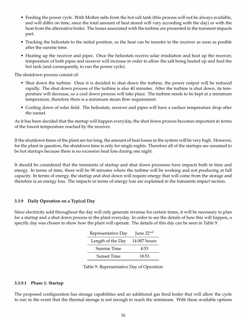
3.3.9 Daily Operation on a Typical Day

Since electricity sold throughout the day will only generate revenue for certain times, it will be necessary to planfor a startup and a shut down process in the plant everyday. In order to see the details of how this will happen, aspecific day was chosen to show how the plant will operate. The details of this day can be seen in Table 9.

Representative Day June 22nd

Length of the Day 14.007 hours

Sunrise Time 4:53

Sunset Time 18:53

Table 9: Representative Day of Operation

3.3.9.1 Phase 1: Startup

The proposed configuration has storage capabilities and an additional gas fired boiler that will allow the cycleto run in the event that the thermal storage is not enough to reach the minimum. With these available options

16

other than the power directly from the solar field, the initial time for full production is set at 5:00. For the dayin question, there is thermal storage in the hot salt tankwhich can be used for the startup of the turbine at this time.

The total startup time for the plant is set at 45 minutes. The most significant portion of this time is devoted to thestartup process of the turbine. The turbine startup time was determined to be 40 minutes 1. The rest of the timeis left for the process of heating the pipes from the hot tank to the heat exchanger (steam generator) to run thepower cycle. It is important to note that if there was no remaining thermal storage at the beginning of the day, thestartup time would change.

Therefore, the the warm-up operations will start at 4:15 to be on schedule to produce full power at 5:00. Thereis no day of the year where there is enough solar irradiance at 4:15 to run the cycle without taking heat fromthe hot salt tank, or from the gas fired boiler. Regarding the solar field, the receiver and pipes along the centraltower require a certain amount of time to reach the minimum temperature and to allow the salt to be heated up.However, this heating process of the receiver will run after the turbine startup process and it will not reduce thepower output.

Due to the tracking systems of the heliostats in the solar field, it can be assumed that the warm-up process ofthe solar receiver will not take a substantial amount of time because all available heat will be concentrated to thiseffort. The initial temperature can be either the ambient temperature or higher 2. Once the receiver has reached ahigher temperature than the cold tank (which is at 290oC), the salt can be pumped to the receiver for the heatingprocess. However, the salt needs to reach 560oC before it can run the power cycle. For this representative day, theminimum required temperature of the receiver to run the cycle, should be achieved by 8:00.

3.3.9.2 Phase 2: Full Operation

Once the receiver temperature has reached 600oC with the incoming solar irradiance, the molten salt flow fromthe cold to the hot tank will first pass through the tower and receiver. The flow will then travel from the hotthermal tank to the power cycle. By keeping the mass flows equivalent, this can be done without incurring anylosses in the amount of heat stored. In the event that more thermal energy is coming in than is necessary to meetthe electricity demand, then the excess can build up in the thermal storage tank. When the electricity is producedwith the energy collected at the solar field, the plant is in its optimal performance. If there is more energy comingfrom the solar field and the storage is full, the excess energy will be wasted. In the Section 3.4 it can be seen thatthe thermal power at the receiver was enough to store a significant amount of energy in the hot tank.

As a last step into this process, it should be seen that since the maximum irradiance to the receiver is reached inthe solar noon, and after that the irradiance will be reduced, there will be a certain point where the irradiancemay not be enough to keep the receiver at the necessary temperature.

3.3.9.3 Phase 3: Operation After Sunset

The time at which the sun sets will define the time when the energy produced will come from the storage insteadof the solar field. If the storage is exhausted, then the auxillary boiler will produce the necessary steam to keeppower cycle in operation.

For June 22nd, the sunset happens at 18:53. From this time onward, another transient phase for the receiver willstart. Once the incoming solar irradiance on the field is no longer enough to heat up the salt to the necessarytemperature, it becomes pointless to keep the heliostats focused on the receiver. Therefore, the heliostats will be

1See Section 3.4 for more information2See Section 3.4 for more details

17

defocused in order to be ready for the next day. The receiver then needs to be drained (it still has some salt inside)and this salt will be directed to the cold tank. At this time, stored heat from the hot tank will feed the cycle. Forthis representative day, there was no need to operate the auxillary boiler.

3.3.9.4 Shutdown

The shut down time for the plant is defined by an automatic shut down process at 22:00 everyday. At 22:00, therewill be no more solar irradiance at any point in the year. For this particular day, the energy needed to produce thesteam at the power cycle comes from the storage reserves. The steam flow to the turbine eventually stops and thepower produced by the turbine drops. A cool down process of the turbine will subsequently start, and the turbinewill have a minimum steam flow requirement throughout the night that will allow to start operations next day.

3.3.9.5 Summary

In summary, the operational strategy follows these guidelines:

• The storage was set according with an optimization method, that accounts for both the energy needs ofthe cycle, and the cost and profitability of the storage. Storage will minimize the impacts on electricitygeneration due to meteorological events, and will allow production when the solar resource is not enough(and therefore will do a much better job of controlling the daily startup process).

• Electricity will be produced only when it is profitable to do so.

• Preventive maintenance can be done during the time intervals where there is no energy production.

• Since the higher selling price of electricity is from 17:00 to 21:00, the optimal performance will be reached ifthe plant is able to deliver full power at these times.

• Hybridization is considered as an option in order to produce when there is not enough solar resource andthere is also a storage deficiency. According to the optimization method developed and explained in Sec-tion 3.2.2, there will be 18 days during the year where this alternative boiler is used to reach the full poweroutput.

• Startup and shut down processes will impact the energy losses throughout the year. Also, due to the dailystartups, the storage optimization becomes a crucial process. And since there is a fixed time for these tran-sients, operation can be planned in a much better way.

3.3.10 Limitations on Receiver

The receiver had some physical constraints that reduced the maximum amount of solar radiation that could beharnessed from the solar field. The maximum heat flux was equal to 1.5 MWth

m2 [22], so considering the area of thereceiver as 805 m2, the heat flux resulted in 1207.5 MWth. Once this limit is reached, defocusing of the mirrorsis done to reduce the incoming heat flux. The nature of the limit is related to the fatigue of the material and thethermal stresses that can be produced by very high heat fluxes.

Therefore, in order to account for this technical limit, a constraint was added to the Matlab code to dump theadditional power and at the same time optimize the storage and hybridization of the plant. It was because of thisconstraint, the turbine of 150MWe capacity was chosen since the turbine installed with higher capacity (250MWe)would be operating at a considerably lower rated power leading to loss of efficiency.

18

3.4 Transients

3.4.1 Impacts of Transients

In terms of the impacts of transients, the following constraints were identified:

• Within the solar field, the temperature of both the heliostats and the solar receiver at the tower will be afunction of the solar irradiance at that time of the day. Therefore, in a situation with no storage, the poweroutput of the cyclewill notmeet theminimum requirement at the start of the day, because the incoming solarradiation in the morning will not be enough. However, if thermal storage were implemented that necessaryheat during startup would be available.

• Throughout the year, there are some cloudy or troublesome weather events that may cause reduction inpower generated in a situation where storage is not implemented. It was identified that for the chosenlocation, there were some drops in solar irradiance that may be related with these types of events. For thesereasons, storage implementation was analyzed in depth.

3.4.2 Tower Receiver Temperature

When analyzing the tower receiver temperature it was deduced that the amount of time required to heat up thereceiver would not impact the power output as long as storage or the hybridization of a gas fired boiler were used.Therefore, there would be no need to wait until enough solar irradiation is available for the receiver to reach theoperational temperature needed to run the power cycle. Despite this fact, it is still important to know the temper-ature at the receiver in order to have an understanding of how long it will take after the sunrise to run the cycleexclusively with incoming concentrated solar radiation.

The receiver can increase by 50oC in 300 seconds after sunrise, and takes 60 seconds to drop 45oC when the solarenergy is no longer concentrated on it [20]. Therefore, the temperature will be related with the input power to thereceiver. It has been determined that the molten salts will operate between the temperatures of 290oC to 565oC.Based on these parameters the receiver temperature had a desired set point of 600oC in order to run the powercycle withmolten salts. The receiver temperature has an upper limit, because if the temperature of the salt reacheslevels higher than 600oC, then salt degradation may occur [21].

The salts will perform optimally at 565oC which coincides with a receiver temperature of 600oC. If the receiver isheated up further than this, the heat transfer efficiency will start to decrease [21]. Ideally, the receiver temperaturewill reach 600oC as soon as possible. The critical parameter to take into account is then the initial temperature ofthe receiver, which can be assumed to be the average ambient temperature of the area. However, in order to keepconsistency with the hot start up conditions, this temperature was set according to the efficiency curve for a solartower plant [21]. This value is 77oC and is the temperature where there is a receiver efficiency of zero, therefore,there is no solar irradiance.

The solar receiver will increase its temperature until 600oC. The heat transfer at that temperature is the maximumheat transfer rate at the receiver. After this point the receiver does not need more heat. In order to avoid very hightemperatures that may damage the receiver or cause degradation of the salt, some heliostats will be need to bedefocused. The receiver has a peak flux limit, or a limit to the amount of thermal power that is transferred fromthe receiver to the salt.

The receiver gives the salt a thermal power of 483 MW with an efficiency of 91%, which means that the requiredheat rate that makes the receiver able to run the cycle is 530.77 MW [17]. If the receiver gets this heat, the salt canbe heated from its base of 290o to it’s ideal performance temperature of 565oC. The area of the receiver was set to

19

be 805.36 m2. In order to estimate the amount of time required to reach the desired temperatures the followingequations were used:

Q = hA∆T

h =Q

A∆T=

530.7692x106[W ]

(805.36466[m2])(600 − 77)[oC]

h = 1260.1186[W

m2C]

Where:

Variable Description Units

Q Heat Going Through the Receiver W

A Area of the Receiver m2

h Heat Transfer Coefficient Wm2C

∆T Temperature Difference oC

Table 10: Variable Definitions

This is the heat transfer coefficient of the receiver for the proposed plant. With this value, the receiver temperaturecurve for the plant can be generated. At 600oC, the salt can be pumped to the receiver to acquire the thermal energyneeded for the Rankine cycle. It is possible to look into the power at the receiver after each hour as well as thetemperature at its surface. When this value is reached, there is no need to use the storage or the alternative boiler.The data for the energy harvested by the receiver and the associated temperatures can be seen in Table 11.

Time Power at the Receiver (MW) Receiver Temperature (oC)

5:00 0 77

6:00 12.11 92.75

7:00 208.11 363.30

8:00 479.52 600 3

9:00 675.27 600

Table 11: Receiver Temperature vs Time

After 8:00 the power required to run the cycle is provided entirely from the field, and from this time forwardthe plant is able to store any amount of excess energy that is collected. Even though more power is being givenby the field, the heat rate needed is only to keep the temperature of the receiver at 600oC. Also at this time thetemperature will allow the heating of the pipes and the maintenance of the salt flow along the receiver.

Figure 8 shows that two hours after the sunrise, the receiver is able to work at full operation and run the cycle.During that interim time, the electricity can be produced with the stored heat or gas boiler. It is important to takeinto account the fact that the heating process of the field can be done simultaneously with the startup process ofthe turbine. However, after the first hour, at 7:00 the temperature is high enough to heat up the salt partially andtogether with the storage reach the needed temperature for the cycle. In a no storage situation the transient losseswould be reflected in a partial load operation. Another interesting observation in Figure 8 is that from 7:00 to 8:00,approximately every 10 minutes the receiver temperature increases by roughly 40oC.

3At 8:00 the temperature reached 623.38oC, but it is kept at 600oC to ensure ideal performance

20

Figure 8: Receiver Temperature vs. Time

The major losses due to transients in the solar field are significant in a no storage situation. If this is the case, thestartup time is longer, and the time of startup and shut down will change everyday. The production will also notbe the maximum when the demand is higher, and it will definitely not be possible to produce from 5:00 to 22:00everyday. The estimation of the losses due to transients becomes much more complex in a no storage situation.Therefore, it is possible to conclude that for the proposed CSP plant, storage will reduce the impacts of transientsrelated with solar field.

3.4.3 Operation of Plant

Due to the fact that any electricity sold between the hours of 22:00 and 5:00 will not generate any revenue for theplant, there will be at least one startup and one cool down everyday. However, a benefit of this is that some of themaintenance can be scheduled during these times throughout the year. This maintenance can be either preventiveor corrective. During these shutdowns, when the plant is not running in full operation, energy still needs to beavailable for the following reasons.

Operational Requirements During Shutdown Periods:

• To keep a minimum steam flow rate at the turbine in order to maintain a minimum temperature.

• To start up the turbine and allow it to reach full operation levels.

• To preheat the receiver, pipes from the hot tank to the receiver, from the receiver to the cold tank, as well thepipes that go to the steam generator. It is also necessary to keep the hot salt tank at a minimum temperaturelevel.

• To track the heliostats from the last position at sunset to the following position at sunrise, so the receiver canbe warmed in an efficient way.

All of these actions require energy and therefore can be viewed as a cost, since that energy would have to be pro-vided for through some sort of hybridization with fossil fuels or an external backup. However, if the plant wereto have storage capabilities, the additional energy that is reserved can be used for these operational needs. Thisrepresents a considerable advantage, since the excess energy would no longer be lost but would be able to aid inthese operational requirements.

Another major advantage of storage is that it helps reduce the shutdowns and subsequent startups of the turbinedue to cloudiness throughout the day. In the event of passing cloud cover, the electricity production can remainconstant by drawing from the thermal storage of the molten salts. Also, having the ability to store some energy

21

when the irradiance is high and then produce and sell electricity later in the day when the price is optimized, canhelp increase the profitability of the plant.

The startup time of the turbine was chosen as a governing parameter during the analysis of the plant. The startupprocess will take longer if the starting temperature of the receiver and other components are at the ambient tem-perature of nighttime in the desert. Therefore, based on using energy for the above operational requirementsduring the shutdown periods, it was assumed that all startups would be "hot startups". Therefore, the key aspectswere considered to estimate the impact due to transients were the startup, cool down, and the energy needed tokeep the salt and plant components at their minimum temperatures.

3.4.4 Energy Needed for Molten Salt

The plant was designed so that during operation, the molten salt will be heated up to 565oC, and after the steamgeneration process the temperature will drop to 290oC. This will then be the temperature of the salts in the coldreserve tank. Heat losses of the storage tanks have been reported to be 1oF (0.55oC) each day Then, it can beassumed that the heat losses at the tanks are not significant and no additional energy needs to be added, since thesalt will not reach a temperature lower than 260oC during the night period [8].

3.4.5 Transients Energy Calculation for Turbine

Depending on the style and manufacturer of the turbine used in the power cycle, the startup time can vary, asseen in Figure 9.

Figure 9: Turbine Start-Up Curve [9]

It can be seen that within a 40 minute window, the model turbines shown were up to full load. Therefore it wasassumed that the plant would also have a turbine running at full load within 40 minutes of startup. However,

22

before the startup process of the turbine, additional time would be needed for the receiver and the heliostats toget into full load conditions as well. Therefore it has been assumed that startup time for the entire plant would be45 minutes [10].

As an example, the startup time can be chosen to be 4:15 and the cool down time at 22:00. Choosing the Siemensturbine from Figure 9, the process can be divided into three steps. For 12 minutes, there is no power output at theturbine. From 12 minutes to 28 minutes, the output power goes from 0% to 97%. Finally from 28 minutes to 40minutes after startup, the power output reaches its full load of 150 MW

The energy produced can be calculated by determining the area under the curve in the power vs. time chart.Therefore, at minute 28 the power output would be 145.5 MW and the function describing the linear relationshipfrom this point would be:

y = 6.6687x

Integrating from minute 12 to minute 28 the total amount of energy produced can be calculated as 19.4 MWh.Calculated in a similar fashion fromminute 28 to minute 40, the energy output would be 0.45 MWh.Therefore thetotal energy for each turbine startup would be 19.85 MWh.

If storage is implemented, then it would be possible to keep the turbine running after sunset and sell the electricitywhen the price is increased. However like previouslymentioned, there is a point where no profitwill be generatedso the turbine will be forced to stop for economic reasons. For this turbine stop, or cool down process, there willbe a similar shape, but with different phases. It can assumed that the over the first 16 minutes of powering downthe power output will be reduced by 97%. Between 16 minutes and 28 minutes the last 3 percent of power outputwill be scaled down [13]. This cool down process can be see in Figure 10.

Figure 10: Turbine Ramp Down Curve

Calculating the power output that is generated but not paid for can be done via:

y = −6.6687x

23

The energy output will be the same as during the start up process. Integrating along the 16 minute process, yieldsa total of 19.4 MWh. In the next 12 minutes the energy output will be 0.45MWh. So, for the stopping process (andconsequently, a partial cool down process) the energy loss is 19.85 MWh.

In total, each day the energy produced by the turbine and not sold would be 39.7 MWh. Over the course of a yearthere will be a total of 14,490.5 MWh (14.49 GWh). This energy lost is equivalent to % of our total output.

In order to knowhowaccurate this answer is, iswas necessary to research the startup losses for existingCSPplants.According with the National Renewable Energy Laboratory of the US Department of Energy, for a 330MW plantwith 3 hours of storage, the losses due to startup processes are around 23 GWh throughout the year. Consideringthe fact that the proposed plant is 45% of that capacity, the losses should be roughly this percentage as well, whichwould result in 10.45 GWh of losses, compared to the predicted losses of 14.49 GWh).

4 The Algorithm Logic

Figure 11 below highlights the logic of the optimization algorithm used to determine the optimal combination ofstorage size and turbine capacity, to give the lowest payback period. The outermost loop of the algorithm iteratesbetween 150, 175 and 250 MW turbine capacities. For each turbine capacity, another loop iterates through storagesizes ranging from 1 to 10 hours, along with an option of zero storage. As Figure 11 shows, within both of theseloops, the algorithm then moves through each day of the year and subsequently, each hour of the day.

As it goes through each hour, it first checks to see if the hour falls within the range of 5:00 to 22:00. If not, accordingto the tariff scheme, there is no opportunity for revenue generation. Outside of that range there is no chance forpower production and is therefore of no interest to the algorithm. If the hour is within the required range, thealgorithm then compares the thermal power output of the plant to the minimum thermal requirement of 427MW.This is done to see how the power produced is to be managed.

24

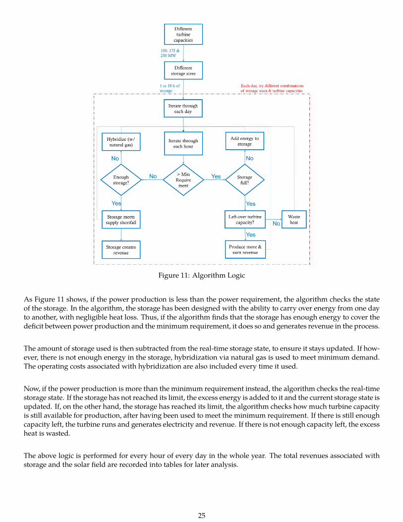
Figure 11: Algorithm Logic

As Figure 11 shows, if the power production is less than the power requirement, the algorithm checks the stateof the storage. In the algorithm, the storage has been designed with the ability to carry over energy from one dayto another, with negligible heat loss. Thus, if the algorithm finds that the storage has enough energy to cover thedeficit between power production and theminimum requirement, it does so and generates revenue in the process.

The amount of storage used is then subtracted from the real-time storage state, to ensure it stays updated. If how-ever, there is not enough energy in the storage, hybridization via natural gas is used to meet minimum demand.The operating costs associated with hybridization are also included every time it used.

Now, if the power production is more than the minimum requirement instead, the algorithm checks the real-timestorage state. If the storage has not reached its limit, the excess energy is added to it and the current storage state isupdated. If, on the other hand, the storage has reached its limit, the algorithm checks howmuch turbine capacityis still available for production, after having been used to meet the minimum requirement. If there is still enoughcapacity left, the turbine runs and generates electricity and revenue. If there is not enough capacity left, the excessheat is wasted.

The above logic is performed for every hour of every day in the whole year. The total revenues associated withstorage and the solar field are recorded into tables for later analysis.

25

4.1 Algorithm Assumptions

One of the assumptions made for this algorithm is that as long as production is between 5:00 and 22:00, the mar-ket would be willing to buy as much electricity as the plant produces, as long as it is more than the minimumrequirement. Another assumption is that the revenue from hybridization is not a part of the optimization algo-rithm. The reason behind this is that hybridization is available as a last-resort, but not as an active part of theplant. Optimizing while including hybridization revenue would skew the results in favor of maximizing naturalgas output and minimizing solar production, which is counter-productive to the overall goal.

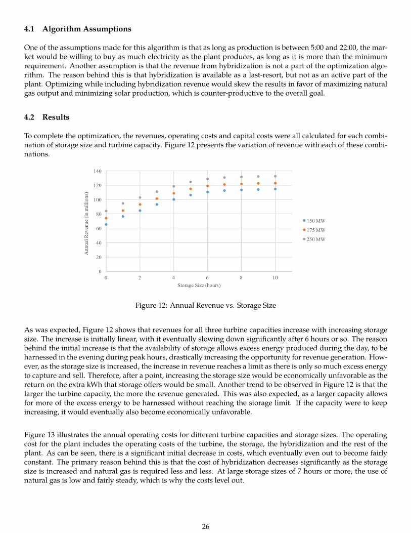
4.2 Results

To complete the optimization, the revenues, operating costs and capital costs were all calculated for each combi-nation of storage size and turbine capacity. Figure 12 presents the variation of revenue with each of these combi-nations.

Figure 12: Annual Revenue vs. Storage Size

As was expected, Figure 12 shows that revenues for all three turbine capacities increase with increasing storagesize. The increase is initially linear, with it eventually slowing down significantly after 6 hours or so. The reasonbehind the initial increase is that the availability of storage allows excess energy produced during the day, to beharnessed in the evening during peak hours, drastically increasing the opportunity for revenue generation. How-ever, as the storage size is increased, the increase in revenue reaches a limit as there is only so much excess energyto capture and sell. Therefore, after a point, increasing the storage size would be economically unfavorable as thereturn on the extra kWh that storage offers would be small. Another trend to be observed in Figure 12 is that thelarger the turbine capacity, the more the revenue generated. This was also expected, as a larger capacity allowsfor more of the excess energy to be harnessed without reaching the storage limit. If the capacity were to keepincreasing, it would eventually also become economically unfavorable.

Figure 13 illustrates the annual operating costs for different turbine capacities and storage sizes. The operatingcost for the plant includes the operating costs of the turbine, the storage, the hybridization and the rest of theplant. As can be seen, there is a significant initial decrease in costs, which eventually even out to become fairlyconstant. The primary reason behind this is that the cost of hybridization decreases significantly as the storagesize is increased and natural gas is required less and less. At large storage sizes of 7 hours or more, the use ofnatural gas is low and fairly steady, which is why the costs level out.

26

Figure 13: Annual Operating Costs vs. Storage Size

Figure 14, shows howmuch hybridization was used in the whole year, and highlights the same trend. The reasonthe amount of hybridization is exactly the same for all three turbines is that hybridization is only used when thesolar field or the storage are not able to reach the minimum requirement. It does not in any way depend on thesize of the turbine itself.

Figure 14: Hybridization Amount vs. Storage Size

The difference in costs for different turbine capacities in Figure 13, are due to different the turbine operating costswhich scale linearly with size. This is why the difference in the curves aligns well with the difference in turbinecapacities.

Figure 15 shows the variation of total annual capital costs with storage sizes and turbine capacities. The capitalcost includes the turbine equipment cost, the storage equipment cost, the hybridization equipment cost and theequipment costs for the rest of the plant. It also includes the cost of project development and site installation. Asall these costs are linearly dependent on the size of the system, they increase linearly with both the storage sizeand the turbine capacity.

27

Figure 15: Capital Costs vs. Storage Size

Given the costs provided before, a non-discounted payback period was then computed for the various storagesizes and turbine capacities. It was maintained as non-discounted, as it was only a means to choose the optimumcombination. From Figure 16, it can be seen that the combination that yields the smallest payback period is a 150MW steam turbine with 7 hours of thermal storage.

Figure 16: Payback Period vs. Storage Size

The choice of 150 MW and 7 hours of storage reflects the most economically feasible choice given the technicalspecifications and constraints of the solar field. This, however, does not mean that it is the most efficient choice.This can be seen in Figure 17, which shows the annual amount of heat wasted for different combinations. As canbe seen, storage does reduce wastage for all turbine capacities, but the losses for a 150MW turbine are around 740GWh while those for a 250 MW turbine are drastically lower, at 45 GWh.

28

Figure 17: Annual Heat Wasted vs. Storage Size

5 Overall Performance of the Plant

From the irradiation over each hour and day of the year, and together with the code developed in Matlab fordimensioning the field, it was possible to calculate the total thermal power output each hour at each cell in thefield. This was done for the total 365 days. Once the power cycle was designed (and therefore the efficiencieswere known), the operative strategies were defined, and the transient losses were considered, the total energyproduced was calculated. The optimization algorithm explained before was also applied.

At this stage, it was also possible to estimate the amount of time where the plant will operate at different times.This will be the base to calculate the revenue and evaluate the profitability of the plant in the next chapter. Thetotal operational hours at the peak time (where the electricity is better paid) and the operational hours at normaltariff were calculated. As explained before, there is no production at the times electricity is not being paid.

The total performance in the proposed CSP plant is summarized in Table 12.

29

Overall Efficiency of the Plant 19.27%

Design Day for Solar Multiple 21st June at Solar Noon

Solar Multiple 1.83

Optimal Storage 7 hours

Total Annual Hybridization Hours 209

Turbine Electrical Power Output 150 MW

Capacity Factor 55.7%

Time of Operation During Peak 1460 hours

Time of Regular Operation 3,321.93 hours

Total Operational Hours 4,781.93 hours

Total Transient Operational Losses 14.5 GWh

Total Annual Electricity Produced 731.78 GWh

Table 12: Total CSP Plant Performance

6 Financial Analysis

6.1 Capital Expenditures (CAPEX)

The capital expenditure and capital investment for a 150MWe solar tower power plant designed in Ouarzazatewas determined to be $652M. The estimated breakdown for the capital expenditure includes the cost of equip-ment, engineering, land, installment, construction, and the plant itself. The cost of engineering, land installment,construction and the plant are based on the total cost of equipment and corresponding factors for each. The factorslisted in Table 13, were established based on information provided by engineers working in the power industry.

Factors

Installation 15%

Engineering 5%

O&M 10%

Construction 13%

Decommissioning 5%

CAPEX 52%

Table 13: Cost Factors

The CAPEX breakdown can be seen in more detail in Figure 18 and Table 14

30

Figure 18: CAPEX

Cost of Equipment $461,745,150.95

Cost of Installment $26,550,346.18

Cost of Engineering $66,375,865.45

Cost of Construction $66,375,865.45

Cost of Land $28,261,000.00

Total $652,194,135.22

Table 14: CAPEX

6.2 Operational Expenditures (OPEX)

The OPEX cost of the plant was estimated to be $2,663,887 per annum. The OPEX was determined using theoperation strategy mentioned earlier in the report. The major cost in OPEX were operation & maintenance, laborand the fuel for hybridization.

Figure 19: OPEX

31

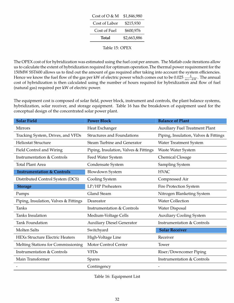
Cost of O & M $1,846,980

Cost of Labor $215,930

Cost of Fuel $600,976

Total $2,663,886

Table 15: OPEX

TheOPEX cost of for hybridizationwas estimated using the fuel cost per annum. TheMatlab code iterations allowus to calculate the extent of hybridization required for optimum operation.The thermal power requirement for the150MW SST600 allows us to find out the amount of gas required after taking into account the system efficiencies.Hence we know the fuel flow of the gas per kW of electric power which comes out to be 0.025 L

sec−kW . The annualcost of hybridization is then calculated using the number of hours required for hybridization and flow of fuel(natural gas) required per kW of electric power.

The equipment cost is composed of solar field, power block, instrument and controls, the plant balance systems,hybridization, solar receiver, and storage equipment. Table 16 has the breakdown of equipment used for theconceptual design of the concentrated solar power plant.

Solar Field Power Block Balance of Plant

Mirrors Heat Exchanger Auxiliary Fuel Treatment Plant

Tracking System, Drives, and VFDs Structures and Foundations Piping, Insulation, Valves & Fittings

Heliostat Structure Steam Turbine and Generator Water Treatment System

Field Control and Wiring Piping, Insulation, Valves & Fittings Waste Water System

Instrumentation & Controls Feed Water System Chemical Closage

Total Plant Area Condensate System Sampling System

Instrumentation & Controls Blowdown System HVAC

Distributed Control System (DCS) Cooling System Compressed Air

Storage LP/HP Preheaters Fire Protection System

Pumps Gland Steam Nitrogen Blanketing System

Piping, Insulation, Valves & Fittings Deareator Water Collection

Tanks Instrumentation & Controls Water Disposal

Tanks Insulation Medium-Voltage Cells Auxiliary Cooling System

Tank Foundation Auxiliary Diesel Generator Instrumentation & Controls

Molten Salts Switchyard Solar Receiver

HEXs Structure Electric Heaters High-Voltage Line Receiver

Melting Stations for Commissioning Motor Control Center Tower

Instrumentation & Controls VFDs Riser/Downcomer Piping

Main Transformer Spares Instrumentation & Controls

- Contingency -

Table 16: Equipment List

32

The levelized cost of electricity based on the capital expenditure, operational expenditure, and annual perfor-mance was 167.45 $

MWh . The following equation was used to calculate the levelized cost of electricity:

LCOE =α ∗ Cinv + Cf + CO&M + β ∗ Cdec

Enet

Where:

Variable Description Units

LCOE Levelized Cost of Electricity $/kWh

Cinv Initial Cost of Investment $

CO&M Costs for Operation and Maintenance $

Cdec Cost for Decommissioning $

n Lifetime of the Power Plant Years

α Annualization Factor -

β Discount Factor -

Table 17: Variable Definitions

Themacro-environmental economic conditions used in the financial analysis of the plant were inflation, corporatetax, and interest on investment for CSP plants. Inflation in Morocco is 0.3% and the corporate tax is set at 8% forforeign contractors completing technical work in engineering, construction or assembly projects [14, 15]. Thelevelized cost of electricity is affected by these macro-environmental economic conditions because it incorporatesa discount and annualization factor that includes the interest rate of an investment and inflation, therefore theLCOE value is decreased. These fiscal conditions of Morocco are important to consider in order to fully assess theviability of the CSP project.

6.3 Tariffs

Proposed schemes for tariffs based on an internal rate of return of 10% can then be seen in Table 18.

Clock Time CSP Tariff ( USDMWh )

00:00 - 05:00 0

05:00 - 17:00 140

17:00 - 21:00 140 x1.4996 = 209.94

21:00 - 22:00 140

22:00 - 24:00 0

Table 18: Final Tariff Structure for CSP Plant

7 Environmental Impacts

In order to evaluate the environmental benefits by producing clean electricity from solar power instead of fossilfuels, the analysis focused in two major indicator; water consumption of the plant and its CO2 emissions.

33

In terms of water consumption, the dry cooling process reduces the water needed of the power cycle andmake upwater requirement also reduces as a result. Since the steam cycle is a closed system, the major water requirementis for cleaning themirrors. The estimatedwater consumption each year is only 55,402 m3

year [28]. Another importantthing is that there is no competition with the nearest population centers. It is also to be noted that once the plant isunder operation, thewater requirement is very low as comparedwith thewater required at the construction stage.

Regarding the CO2 emissions, the proposed power plant has CO2 emission of 1.88 kg CO2eqMWh . In total, the CO2

emissions are 1,375.07 tons. If the same amount of electricity was to be generated using natural gas, the emissionswould be 404,956 tons. And if the electricity was to be produced with a coal power plant, the total emissionswould be 697,098 tons. It is possible to conclude that the proposed CSP plant has a significant environmentalbenefits. In the graph below is clearly seen that a CSP plant is a very good alternative in terms of climate changemitigation. The detailed calculations are attached in the appendix.

Figure 20: Avoided Emissions

8 Conclusion

The proposed CSP plant had an overall sun-to-electricity efficiency of 19.27% and an annual electricity produc-tion of 731.78 GWh. The final payback period was determined to be 10 years, making this project economicallyfeasible. The Levelized Cost of Electricity was 167.45 USD

MWh , allowing for a competitive tariff scheme for electricitydistribution.

The optimization algorithm determined that a combination of 150 MW and 7 hours of molten salt storage, wouldgive the most viable power plant. The presence of storage proved to be hugely beneficial to the power plant, asit allowed the plant to store excess energy during the day and use it during peak periods, generating sizable rev-enues as a result.

The presence of storage also hadmajor environmental benefits, as it significantly reduced the amount of hybridiza-tion employed the plant. Overall, the plant ends up reducing carbon emissions by 403,500 tons. Also, the powerplant consumes relatively less water, with annual consumption at 55,402m3.

Hence, the proposed power tower CSP plant is a great solution as it manages to exceed the minimum technicalrequirement while being economically feasible to an investor, and environmentally friendly.

34

9 References

[1] Specimen NewsWorld’s Largest Concentrated Solar Power Plant Installed in Moroccohttp://specimennews.com/2016/02/05/worlds-largest-concentrated-solar-power-plant-installed-in-morocco/Date Published: February 5, 2016Date Accessed: February 25, 2016

[2] CNNWorld’s Largest Concentrated Solar Plant Switches on in the Saharahttp://edition.cnn.com/2016/02/08/africa/ouarzazate-morocco-solar-plant/Date Published: February 8, 2016Date Accessed: February 27, 2016

[3] AIChE - ChEnectedKing of Morocco Plans to Export Solar Power to Europehttp://www.aiche.org/chenected/2016/02/king-morocco-plans-export-solar-power-europeDate Published: February 19, 2016Date Accessed: February 27, 2016

[4] NRELParabolic Trough Solar Field Technologyhttp://www.nrel.gov/csp/troughnet/solar_field.htmlDate Published: January 28, 2010Date Accessed: February 27, 2016

[5] Solar TowerMeteorological Reactorshttp://www.solar-tower.org.uk/quick-start.phpDate Accessed: February 27, 2016

[6] SoDaTime Series of Solar Radiation Datahttp://www.soda-is.com/eng/services/services_radiation_free_eng.phpDate Published: October 2, 2015Date Accessed: February 27, 2016

[7] CSP TodayTMY - Typical Meteorological Year - What Should it Represent and What Means P50, P70, and P90http://social.csptoday.com/technology/tmy-%E2%80%93-typical-meteorological-year-what-should-it-represent-and-what-means-p50-p70-and-p90Date Published: March 7, 2011Date Accessed: March 1, 2016

[8] Solar ReserveMolten Salt Energy Storagehttp://www.solarreserve.com/en/technology/molten-salt-energy-storage

35

Date Accessed: March 2, 2016

[9] WärtsiläCombustion Engine vs Gas Turbine: Startup Timehttp://www.wartsila.com/energy/learning-center/technical-comparisons/combustion-engine-vs-gas-turbine-startup-timeDate Accessed: March 2, 2016

[10] ACWA PowerNoor III Tower CSP Plant, Ouarzazate, Morocco Specific Environmental and Social Impact AssessmentVolume 1 pg. 47 - 52http://www.masen.org.ma/upload/environnement/Masen_NOORoIII_SESIA_Volume_1Main_Text.pdfDate Published: March 2015Date Accessed: March 2, 2016

[11] KTH Bilda - SPG ExercisesSteam Cyclehttps://bilda.kth.se/courseId/12692/content.do?id=24482514Date Accessed: March 2, 2016

[12] Chalmers UniversityMethods of Increasing Thermal Efficiency of a Counter Flow Air to Air Heat ExchangerAuthors: Karl Larsson and Fredrik Pihlquist http://publications.lib.chalmers.se/records/fulltext/145340.pdfDate Published: 2011Date Accessed: March 2, 2016

[13] Transactions of the Institute of Fluid-Flow MachineryMethods of Increasing Thermal Efficiency of a Counter Flow Air to Air Heat Exchanger pg. 175Author: Mariusz Banaszkiewicz http://yadda.icm.edu.pl/yadda/element/bwmeta1.element.baztech-484a0f98-081c-46a9-8716-cb06f56ffc03/c/Trans169-198.pdfDate Published: October 15, 2014Date Accessed: March 4, 2016

[14] Trading EconomicsMorocco Inflation Ratehttp://www.tradingeconomics.com/morocco/inflation-cpiDate Accessed: March 5, 2016

[15] Santander Trade PortalMorocco: Tax Systemhttps://en.santandertrade.com/establish-overseas/morocco/tax-systemDate Published: 2016Date Accessed: March 5, 2016

[16] KTHDesign of Solar Tower CSP PlantsAuthor: Rafael E. GuédezRenewable Energy Technology - Advanced Course Lecture Slides

36

Date Published: January 22, 2016Date Accessed: March 6, 2016

[17] KTHProject Description and GuidelinesAuthor: Concentrating Solar Power GroupRenewable Energy Technology - Advanced Course Project DescriptionDate Published: February 2016Date Accessed: March 6, 2016

[18] KTHHeliostat Design pg. 22Master of Science Thesis Author: Nils Björkmanhttp://www.diva-portal.se/smash/get/diva2:769446/FULLTEXT01.pdf Date Published: 2014Date Accessed: March 6, 2016

[19] Power from the SunCentral Receiver Systemshttp://www.powerfromthesun.net/Book/chapter10/chapter10.html Date Accessed: February 27, 2016

[20] Science DirectTransient Analysis of a Molten Salt Cavity Receiver pg. 604Authors: Q.Q. Zhang, X. Li, C. Chang, H. Liu, Z.F. Wanghttp://ac.els-cdn.com/S1876610214005190/1-s2.0-S1876610214005190-main.pdf?_tid=184d90de-e3c9-11e5-a927-00000aab0f02&acdnat=1457289034_d982356116d99fc80c4731759896fa3fDate Published: 2013Date Accessed: February 28, 2016

[21] DLRReceivers for Solar Tower SystemsAuthor: Prof. Dr. Bernhard Hoffschmidthttp://sfera2.sollab.eu/uploads/images/networking/SFERA%20SUMMER%20SCHOOL%202014%20-%20PRESENTATIONS/SolarTowerReceivers%20-%20Bernhard%20Hoffschmidt.pdfDate Published: June 27, 2014Date Accessed: March 6, 2016

[22] École Polytechnique Fédérale de LausanneThermo-Economic Optimisation of Large Solar Tower Power PlantsAuthor: Germain Augsburgerhttp://infoscience.epfl.ch/record/183139/files/EPFL_TH5648.pdfDate Published: January 24, 2013Date Accessed: March 6, 2016

[23] CSP TodayMorocco’s First CSP Plant Forges Path to Tech-led Cost Cutshttp://social.csptoday.com/markets/moroccos-first-csp-plant-forges-path-tech-led-cost-cutsDate Published: December 2, 2015Date Accessed: March 6, 2016

37

[24] Invest in MoroccoElectricity Tariffshttp://www.invest.gov.ma/index.php?Id=34503&lang=enDate Accessed: March 6, 2016

[25] SiemensSiemens Steam Turbine SST-600http://www.energy.siemens.com/br/en/fossil-power-generation/steam-turbines/sst-600.htmDate Accessed: March 6, 2016

[26] SiemensSiemens Steam Turbine SST-700http://www.energy.siemens.com/hq/en/fossil-power-generation/steam-turbines/sst-700.htmDate Accessed: March 6, 2016

[27] SiemensSiemens Steam Turbine SST-900http://www.energy.siemens.com/mx/en/fossil-power-generation/steam-turbines/sst-900.htmDate Accessed: March 6, 2016

[28] Solar Energy Industries AssociationWater Use Managementhttp://www.seia.org/policy/power-plant-development/utility-scale-solar-power/water-use-managementDate Accessed: March 6, 2016

38

Appendices

Figure 21: Financial Metrics 1

39

Figure 22: Financial Metrics 2

Figure 23: Power Block

40

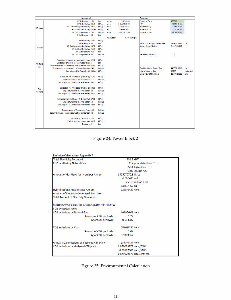
Figure 24: Power Block 2

Figure 25: Environmental Calculation

41

1 %CSP Tower Calcu la t ion S c r i p t2

3 Nrows=8760; %input4 inputf i lename = ’ So lar Values_v05_2005 . csv ’ ; %input5

6 num_helio =8177; %number of h e l i o s t a t s in so l a r f i e l d7 h_T=163 . 2 ; %height of tower (m)8 D_reciever =15 . 16 ; %diameter of r e c e i ve r on tower (m)9 A_tota l =5 .79∗10^6 ; %t o t a l land area required (m2) ? source

10 TES_D=30 . 07 ; %diameter of thermal s torage tank (m)11 Azi_Zones =12; %number of azimuthal zones12 Rad_Zones=12; %number of r ad i a l zones13

14 A_TES=(TES_D/2)^2∗pi ∗2 ; %area of TES tanks (m2)15 A_PowerBlock=A_TES ; %area required for Power Block (m2) ? Tower Area not included

in power block ?16 A_Tower=( D_reciever /2)^2∗pi ; %land area required for Tower (m2)17

18 A_Inner=(A_TES+A_PowerBlock+A_Tower ) ∗ 1 . 5 ; %Area of the inner c i r c l e (m2) ? Reasonfor 1 . 5

19 r_Inner=sq r t ( ( A_Inner )/pi ) ; %radius of the inner c i r c l e (m)20 A_SolarFie ld=A_total −((A_TES+A_PowerBlock+A_Tower ) ∗ 1 . 5 ) ; %Area of the so l a r f i e l d

(m2)21 r_Outer=sq r t ( ( A_tota l )/pi ) ; %raidus of the en t i r e so l a r f i e l d (m)22

23 Stepwidth =( r_Outer−r_Inner ) /12; %Height of a s ing l e c e l l24

25 he l io_dens i ty = [ 0 . 8 3 ; 0 . 7 8 7 5 ; 0 . 7 4 5 0 ; 0 . 7 0 2 5 ; 0 . 6 6 0 0 ; 0 . 6 1 7 5 ; 0 . 5 7 5 0 ; 0 . 5 3 2 5 ;0 . 4 9 0 0 ; 0 . 4 4 7 5 ; 0 . 4 0 5 0 ; 0 . 3 6 2 5 ] ; %setup a blank vec tor fo r the h e l i o s t a t f i e l ddens i ty

26

27 % hel io_dens i ty = [ ] ; %setup a blank vec tor fo r the h e l i o s t a t f i e l d densi ty28 % for r_H=( r_Inner+Stepwidth /2) : Stepwidth : ( r_Outer−Stepwidth /2) %rad i a l d i s tance (

m)29 % hel io_dens i ty =[ he l io_dens i ty ; 0 .721∗ exp (−0 .29∗ ( r_H/h_T ) +0 .03 ) ] ; %h e l i o s t a t

f i e l d densi ty30 % end31

32 Cell_Height =( r_Outer−r_Inner ) /12; %height of each c e l l in a r ad i a l d i r e c t i on (m)33

34 A_cel l = [ ] ; %setup a blank vector fo r the areas of each c e l l in a r ad i a l d i r e c t i on35 r _ c e l l =[ r_Inner+Cell_Height : Cel l_Height : r_Outer ] ; %spe c i f i y the radius of a

s p e c i f i c r ing of c e l l s36

37 fo r i =1:11 %for loop for c a l cu l a t i ng the area of each r ing of c e l l s38 A_cel l ( 1 ) =( r _ c e l l ( 1 ) ^2∗pi−(A_Inner ) ) /12; %ca l cu l a t i ng the area of the f i r s t

r ing39 A_cel l ( i +1) =( r _ c e l l ( i +1)^2∗pi−r _ c e l l ( i ) ^2∗pi ) /12; %ca l cu l a t i ng the area of

subsequent r ings40 end41

42 A_cel l ; %Area of 1 c e l l in each r ad i a l zone43

42

44 A_he l io_ce l l=he l io_dens i ty . ∗ t ranspose ( A_cel l ) ; %area of he l i o s t a t s in 1 c e l l in ar ad i a l r ing

45

46 E_surface =0 . 9 2 ∗0 . 9 66 ; %ca l cu l a t i on of sur face e f f i c t i v e n e s s with re f e rence values47 f_shad =0 . 05 ; %shadowing f a c t o r − given in l e c t u r e s l i d e s48 f_b lock =0 . 0 5 ; %blocking f a c t o r − given in l e c t u r e s l i d e s49

50 h_Helio =6; %height of a h e l i o s t a t from the ground to the panel sur face ( ca l cu l a t edvia s ca l i ng assumption )

51

52 d_r=sq r t ( r _ c e l l .^2+(h_T−h_Helio ) . ^2 ) ; %d i r e c t d i s tance from tower to h e l i o s t a t (d i s tance l i g h t w i l l t r av e l )

53

54 f _ a t t =0.99326−0.1046∗ ( d_r /1000) + ( 0 . 0 17∗ ( d_r /1000) . ^2 ) − (0 .002845∗ ( d_r /1000) . ^3 ) ; %at tenua t ion l o s s e s c o e f f i c i e n t s found from powerfromthesun . net

55

56 %−−−− Sunay −−−−−;57

58 % Importing so l a r i r r ad i ance data a t hourly l ev e l59 f i l e ID = fopen ( inputf i lename ) ;60 so la r_da ta = tex t s can ( f i l e ID , ’%f %f %f %f %f %f %f %f %f %f %f %f %f %f ’ , ’

Del imi ter ’ , ’ , ’ , ’ Headerl ines ’ , 1 ) ;61 f c l o s e ( f i l e ID ) ;62

63 %Cosine E f f e c t i v ene s s Ca lcu la t ion64 %1 . Vs vec tor − 16800x3 matrix65 so la r_da ta { : , 1 5 } = −s in ( so la r_da ta { : , 1 3 } ) . ∗ cos ( so la r_da ta { : , 1 4 } ) ;66 so la r_da ta { : , 1 6 } = −s in ( so la r_da ta { : , 1 3 } ) . ∗ s in ( so la r_da ta { : , 1 4 } ) ;67 so la r_da ta { : , 1 7 } = cos ( so la r_da ta { : , 1 3 } ) ;68

69 v_s = [ so la r_da ta { : , 1 5 } so la r_da ta { : , 1 6 } so la r_da ta { : , 1 7 } ] ;70

71 %2 . Vt vec tor − 144x5 matrix72

73 theta_T = atan ( ( h_T−h_Helio ) ./ r _ c e l l ) ; %for each 12 r ad i a l zones74 theta_H = [ pi /12: pi /6:2∗ pi−pi /12 ] ; %per r ad i a l zone , fo r each 12 azimuthal zones75 v_T = [ ] ;76 pos i t ion_dependent_ fac tors = ( A_he l io_ce l l . ∗ ( f _ a t t ’ ) ) ’ ; %depends on rad i a l

pos i t i on77

78 fo r i =1 : 1 2 ;79 fo r j =1 : 1 2 ;80 temp_T = [ r _ c e l l ( i ) theta_H ( j ) s in ( theta_H ( j ) ) . ∗ cos ( theta_T ( i ) ) −s in (

theta_H ( j ) ) . ∗ cos ( theta_T ( i ) ) s in ( theta_T ( i ) ) pos i t ion_dependent_ fac tors( i ) ] ;

81 v_T = [ v_T ; temp_T ] ;82 end ;83 end ;84

85 %3 . NH vector − (16800 x144 ) x3 matrix86

87 vs_vt = zeros (Nrows∗144 ,4 ) ; %CHANGE IT ACCORDING TO EXCEL88 NH = zeros (Nrows∗144 ,3 ) ; %CHANGE IT ACCORDING TO EXCEL

43

89

90 fo r i =1:Nrows ; %Change 12 to 16800/2 − Do i t only fo r 2004 , no need to c a l cu l a t esepara te ly fo r 2005

91 fo r j =1 : 144 ;92 vs_vt ( ( i −1)∗144+ j , : ) = [ v_s ( i , 1 ) +v_T ( j , 3 ) v_s ( i , 2 ) +v_T ( j , 4 ) v_s ( i , 3 ) +v_T

( j , 5 ) sq r t ( ( v_s ( i , 1 ) + v_T ( j , 3 ) ) ^2+(v_s ( i , 2 ) +v_T ( j , 4 ) ) ^2+(v_s ( i , 3 ) +v_T ( j, 5 ) ) ^2) ] ;

93 NH( ( i −1)∗144+ j , : ) = [ vs_vt ( ( i −1)∗144+ j , 1 ) ./ vs_vt ( ( i −1)∗144+ j , 4 ) vs_vt ( ( i−1)∗144+ j , 2 ) ./ vs_vt ( ( i −1)∗144+ j , 4 ) vs_vt ( ( i −1)∗144+ j , 3 ) ./ vs_vt ( ( i −1)∗144+ j , 4 ) ] ;

94 end ;95 end ;96

97 %4 . Cosine E f f e c t i v ene s s − Dot Product of v_T and NH;98

99 v_T_for_dot = [ v_T ( : , 3 ) v_T ( : , 4 ) v_T ( : , 5 ) ] ;100 E_cosine = ones (Nrows , 1 ) ;101

102 fo r i =1:Nrows ;%Change 12 to 16800/2 − Do i t only fo r 2004 , no need to c a l cu l a t esepara te ly fo r 2005

103 fo r j =1 : 144 ;104 E_cosine ( ( i −1)∗144+ j ) = [ abs ( dot ( v_T_for_dot ( j , : ) , NH( ( i −1)∗144+ j , : ) )/

sq r t ( v_T_for_dot ( j , 1 ) ^2 + v_T_for_dot ( j , 2 ) ^2 + v_T_for_dot ( j , 3 ) ^2) ) ] ;105 end ;106 end ;107

108 %5 . Merging ( Horizontal Concatenation ) Cosine E f f e c t i v ene s s with So lar Data ;109 temp_data = [ so la r_da ta { : , 1 } so la r_da ta { : , 2 } so la r_da ta { : , 3 } so la r_da ta { : , 4 }

so la r_da ta { : , 5 } so la r_da ta { : , 6 } so la r_da ta { : , 7 } ] ;110 master_data = zeros (Nrows∗144 ,11 ) ;111 f o r i =1:Nrows ;%Change 12 to 16800/2 − Do i t only fo r 2004 , no need to c a l cu l a t e

separa te ly fo r 2005112 f o r j =1 : 144 ;113 master_data ( ( i −1)∗144+ j , : ) = [ temp_data ( i , : ) v_T ( j , 1 ) v_T ( j , 2 ) v_T ( j , 6 )

E_cosine ( ( i −1)∗144+ j , 1 ) ] ;114 end ;115 end ;116

117 %Fie ld power c a l cu l a t i on s118 f _ s p i l l = 0 . 0 2 8 4 ;119 t ime_independent_factors = E_surface ∗(1− f_shad ) ∗(1− f_b lock ) ∗(1− f _ s p i l l ) ;120 master_data ( : , 1 2 ) = t ime_independent_factors ( : , 1 ) . ∗ master_data ( : , 5 ) . ∗ master_data

( : , 1 0 ) . ∗ master_data ( : , 1 1 ) ; %master_data ( : , 1 0 ) i s the pos i t i on dependent f a c t o rand master_data ( : , 1 1 ) i s cos ine e f f e c t i v en e s s

121 Power_Cel l_he l ios ta t = master_data ;122

123 Helio_Densi ty_Area_rat io = he l io_dens i ty . ∗ A_cell ’ . / A_he l io_ce l l ; % turns out to beunity always

124 Power_field = Power_Cel l_he l ios ta t ;125

126 %Ef f i c i en cy of CSP Plants − Taking re f e rence from PPT and subs t an t i a t i ng i t127 %from ht tps ://www. i rena . org/DocumentDownloads/Pub l i ca t i ons/IRENA−ETSAP%20Tech%20

B r i e f%20E10%20Concentrat ing%20Solar%20Power . pdf

44

128

129 Inc ident_Solar_Energy = 2319 . 9 ;130 Net_Energy = 3 8 0 . 9 ;131 %Net_Ef f i c i ency = Net_Energy/Incident_Solar_Energy ;132 Net_Ef f i c i ency = 0 . 7 5 ;133

134 %Net Power Output from the CSP Plant135 P_elec_output = Power_field ;136 P_elec_output ( : , 1 2 ) = Net_Ef f i c i ency ∗P_elec_output ( : , 1 2 ) ;137

138 P_elec_output_f = num2cell ( P_elec_output ) ;139 P_elec_output_f = ve r t c a t ( { ’ Year ’ ’Month ’ ’Day ’ ’Time ’ ’ I r r ad iance ’ ’

Lower bound ’ ’Upper bound ’ ’ Radial Pos i t i on ’ ’ Azimuthal Pos i t i on ’ ’ Pos i t i ondep f a c t o r s ’ ’ Cosine E f f e c t i v ene s s ’ ’Net Power Output ’ } , P_e lec_output_f ) ;

140

141 f i d = fopen ( ’ So lar Thermal Power Output . csv ’ , ’w’ ) ;142 f p r i n t f ( f id , ’%s , ’ , P_e lec_output_f { 1 , 1 : end } ) ;143 f p r i n t f ( f id , ’%s\n ’ , P_e lec_output_f { 1 , end } ) ;144 f c l o s e ( f i d ) ;145 dlmwrite ( ’ So lar Thermal Power Output . csv ’ , P_e lec_output_f ( 2 : end , : ) , ’−append ’ )146

147 %−−−− Sunay −−−−−;

1 %Running the whole year of 2005 through the s torage opt imizat ion code2

3 %Importing the f i l e requested and putt ing i t in to an array4 f i d = fopen ( ’ So lar Thermal Power Output . csv ’ ) ;5 input_arr = tex t s can ( f id , ’%f %f %f %f %f %f %f %f %f %f %f %f ’ , ’ Del imi ter ’ , ’ , ’ , ’

Headerl ines ’ , 1 ) ;6

7 %Only ex t r a c t i ng the year , month , day , time and net power output from8 %the f i e l d9 power_output_arr = [ input_arr { 1 } , input_arr { 2 } , input_arr { 3 } , input_arr { 4 } ,

input_arr { end } ] ;10

11 %I n i t i a l i z a t i o n12 s t r t _ i ndx = 1 ;13 new_arr = ones ( 8760 , 5 ) ;14 count = 0 ;15

16 %Combining the power outputs of 144 c e l l s fo r each hour in to one s ing l e17 %value18 while s t r t _ i ndx < length ( power_output_arr )19 count = count +1;20 temp_arr = power_output_arr ( s t r t _ i ndx : s t r t _ i ndx +143 , : ) ; %s p l i t t i n g the rows

in to hours , by i t e r a t i n g through every 144 rows (which are the number ofc e l l s )

21 new_arr ( count , : ) = [ temp_arr ( 1 , 1 : 4 ) , sum( temp_arr ( : , 5 ) , 1 ) ] ; %making a newarray tha t imports the ( year , month , day , time ) stamp along with the sum ofpower outputs from a l l c e l l s fo r tha t hour

22 s t r t _ i ndx = s t r t _ i ndx + 144 ;23 end24

45

25 %I n i t i a l i z a t i o n26 previous_day = 1 ;27 P_out_dai ly = 0 ;28 day_count = 1 ;29 days_arr = c e l l ( 3 65 , 1 ) ;30 operat ion_count = 0 ;31

32 %Breaking up the hour−wise array in to a day−wise c e l l array with each day33 %in i t s own c e l l34 fo r i = 1 : length ( new_arr )35 today = new_arr ( i , 3 ) ;36 i f new_arr ( i , 5 ) >0 %checking how many hours the plant (minus s torage ) i s

operat ing for37 operat ion_count = operat ion_count + 1 ;38 end39 i f abs ( today − previous_day ) >0 || i== length ( new_arr ) %i f we move to the next

day now, s to r e the previous day ’ s data . Or i f we’ re a t the end of the f i l e40 i f i < length ( new_arr )41 day_count = day_count +1;42 end43 days_arr { day_count , 1 } = [ days_arr { day_count , 1 } ; new_arr ( i , : ) ] ;44 e l s e45 days_arr { day_count , 1 } = [ days_arr { day_count , 1 } ; new_arr ( i , : ) ] ;46 end47 previous_day = today ;48 end49

50 %I n i t i a l i z a t i o n51 minimum_req = 427 ; %in Thermal MWh, minimum requirement fo r an hour52 minimum_elec = 110 ; %in E l e c t r i c MWh, minimum requirement fo r an hour , fo r s e l l i n g

.53 the rmtoe l e c_ ra t i o = minimum_elec/minimum_req ; %Thermal to e l e c t r i c54 storage_revenue = 140 ; %$/MWh, earned from s to r ing and s e l l i n g the e l e c t r i c i t y55 plant_revenue = 140 ; %$/MWh, earned from producing and s e l l i n g the e l e c t r i c i t y56 hybrid_cost = 40 ; %$/MWh, cos t of hybr id iza t ion cos t57 date_s tore = ones ( 3 65 , 3 ) ;58 s torage_waste_s tore = [ ] ;59 max_heat = 0 . 75∗1083 ; %in MWH, maximum heat60

61 turbine_vec = [150 , 175 , 2 5 0 ] ;%d i f f e r e n t turb ine s i z e s fo r opt imizat ion , in MW62

63 %We’ l l need these vec tors a t the end64 master_s tore = ones ( 365 , 33 ) ;65 hybr id_s tore = ones ( 365 , 33 ) ;66 hybr id_cos t_s tore = ones ( 365 , 33 ) ;67 e l e c _ s t o r e = ones ( 365 , 33 ) ;68 hybrid_revenue_store = ones ( 365 , 33 ) ;69 s torage_waste_s tore = ones ( 365 , 33 ) ;70 no_stg_hyb_store = ones ( 365 , 33 ) ;71

72 column_count = 0 ;73 hybrid_amount = 0 ;74 hybrid_hours = 0 ;

46

75

76 fo r turb ine_capac i ty = turbine_vec %i t e r a t i n g for d i f f e r e n t turb ine s i z e s andc apa c i t i e s

77 fo r s to rage_s i ze = 0 :10 %i t e r a t i n g between 1 and 10 hours of s torage78 stuff_happened = 0 ;79 column_count = column_count +1;80 s t o r age_ l im i t = s to rage_s i ze ∗ minimum_req ; %in Thermal MWh, the maximum

amount the s torage can have81

82 %Going through each day of the year83 fo r each_day = 1 : length ( days_arr )84 hour_arr = days_arr { each_day , 1 } ; %ex t r a c t i ng the hour−by−hour

information for tha t day85

86 %For the f i r s t day of the year87 i f each_day==188 %I n i t i a l i z a t i o n89 storage_accum = 0 ; %the amount of thermal MWh in the s torage r i gh t

now, i t ’ s cons tan t ly accumulating90 t o t a l _hybr id_cos t = 0 ; %t o t a l cos t of hybr id iza t ion91 to ta l_s torage_revenue = 0 ; %t o t a l revenue earned from s e l l i n g

e l e c t r i c i t y from storage92 to ta l_p lan t_revenue = 0 ; %t o t a l revenue earned from s e l l i n g

e l e c t r i c i t y from the plant93 storage_waste = 0 ; %how much excess energy can ’ t be s tored as

s torage i s f u l l94 to ta l_e l ec_prodn = 0 ;95 to ta l_hybr id_revenue = 0 ;96 no_stg_hyb_count = 0 ;97

98 %I t e r a t i n g through each hour of the day99 fo r each_hour = 1 : length ( hour_arr )

100 time_hour = hour_arr ( each_hour , 4 ) ; %tha t pa r t i c u l a r hour ofthe day

101 power_hour = ( hour_arr ( each_hour , 5 ) ) /(10^6) ; %Thermal power , inMWh, fo r tha t hour

102

103 i f power_hour > max_heat104 power_hour = max_heat ;105 end106

107 %Only enter ing in tha t period when we’ re ge t t ing money for i t108 i f each_hour >= 5 && each_hour <=22109 i f each_hour >=17 && each_hour <=21110 alpha = 1 . 4 9 7 ;111 e l s e i f each_hour == 22112 alpha = 1 ;113 e l s e i f each_hour >= 5 && each_hour <17114 alpha = 1 ;115 e l s e116 alpha = 0 ;117 end118

47

119 %I f there was more power produced than required , i t i ss tored

120 i f power_hour > minimum_req121

122 storage_accum = storage_accum + ( power_hour −minimum_req ) ; %Excess thermal power i s s tored

123 to ta l_p lan t_revenue = to ta l_p lan t_revenue +minimum_req∗ alpha ∗ the rmtoe l e c_ ra t i o ∗plant_revenue ;

124 tu rb ine_ le f t _ to_produce = turb ine_capac i ty −minimum_elec ; %how much the e l e c t r i c MWh can theturb ine s t i l l produce , given i t produces theminimum amount f i r s t

125

126 to ta l_e l ec_prodn = to ta l_e lec_prodn + minimum_elec ;127

128 i f s t o rage_s i ze == 0129 s t o r age_ l im i t = 10^6;130 storage_accum = 0 ;131 end132

133 %i f the amount of s torage exceeds how much the134 %storage l im i t i s135 i f storage_accum > s to r age_ l im i t136 s torage_excess = storage_accum − s t o r age_ l im i t ; %

how much heat can ’ t be s tored137 to ta l_was te = ( s torage_excess ∗ the rmtoe l e c_ ra t i o )−

tu rb ine_ le f t _ to_produce ; %how much of the "waste " heat w i l l not be harnessed by theturb ine

138

139 i f to ta l_was te >= 0 %in the case where the turb inei s not able to harness a l l the waste heat/ j u s table to harness i t

140 to ta l_p lan t_revenue = to ta l_p lan t_revenue + (turb ine_ le f t _ to_produce ∗plant_revenue ) ;

141 to ta l_e l ec_prodn = to ta l_e lec_prodn +turb ine_ le f t _ to_produce ;

142 storage_waste = storage_waste + to ta l_was te/the rmtoe l e c_ ra t i o ;

143

144 e l s e %in the case where the waste heat i s l e s sthan the capac i ty l e f t over in the turb ine

145 to ta l_p lan t_revenue = to ta l_p lan t_revenue + (s torage_excess ∗ the rmtoe l e c_ ra t i o ∗plant_revenue ) ;

146 to ta l_e l ec_prodn = to ta l_e lec_prodn + (s torage_excess ∗ the rmtoe l e c_ ra t i o ) ;

147 end148 storage_accum = s to r age_ l im i t ; %s e t t i n g the amount

of s torage back to the l im i t i s supposed to bea t

149 end150

48

151 %I f there isn ’ t enough power production and i f s torage hasenough to meet tha t d e f i c i t

152 e l s e i f power_hour < minimum_req && storage_accum > (minimum_req−power_hour )

153 storage_accum = storage_accum − (minimum_req−power_hour ) ; %the d e f i c i t fo r tha t hour i s removedfrom the accumulated s torage

154 to ta l_s torage_revenue = to ta l_s torage_revenue + ( (minimum_req−power_hour ) ∗ the rmtoe l e c_ ra t i o ∗storage_revenue ) ; %revenue from storage fo r f i l l i n gtha t d e f i c i t

155 to ta l_p lan t_revenue = to ta l_p lan t_revenue + power_hour∗ the rmtoe l e c_ ra t i o ∗plant_revenue ; %revenue frome l e c t r i c i t y production

156

157 to ta l_e l ec_prodn = to ta l_e lec_prodn + minimum_elec ;158 no_stg_hyb_count = no_stg_hyb_count + 1 ;159 e l s e160 hybrid_amount = hybrid_amount + (minimum_req −

power_hour ) ∗ the rmtoe l e c_ ra t i o ; %amount ofhybr id iza t ion

161 t o t a l _hybr id_cos t = to t a l _hybr id_cos t + (minimum_req −power_hour ) ∗ hybrid_cost ; %cos t of hybr id iza t ion

162 hybrid_hours = hybrid_hours + 1 ;163 to ta l_hybr id_revenue = tota l_hybr id_revenue + ( (

minimum_req − power_hour ) ∗ the rmtoe l e c_ ra t i o ∗plant_revenue ) ;

164

165 to ta l_e l ec_prodn = to ta l_e lec_prodn + minimum_elec ;166 no_stg_hyb_count = no_stg_hyb_count + 1 ;167 end168 end169 end170

171 %Now th i s looks a t every day bes ides the f i r s t one172 e l s e173 power_prodn_vec = hour_arr ( : , 5 ) ; %vector with a l l the hourly power

production174 non_zero_prodns = f ind ( power_prodn_vec~=0) ; %f inding the f i r s t non

−zero hour of power production175 s tr t_prodn_t ime = non_zero_prodns ( 1 ) ; %f inding tha t hour of f i r s t

non−zero power production176

177 s t r t_prodn = ( hour_arr ( str t_prodn_time , 5 ) ) /(10^6) ; %productionduring f i r s t hour of sunshine

178 i f s t r t_prodn > max_heat179 s t r t_prodn = max_heat ;180 end181

182 i f s t r t_prodn < minimum_req %i f there isn ’ t enough powerproduction in the f i r s t hour of sunshine

183 %going through the hours in tha t day , un t i l production184 %goes above the minimum amount required

49

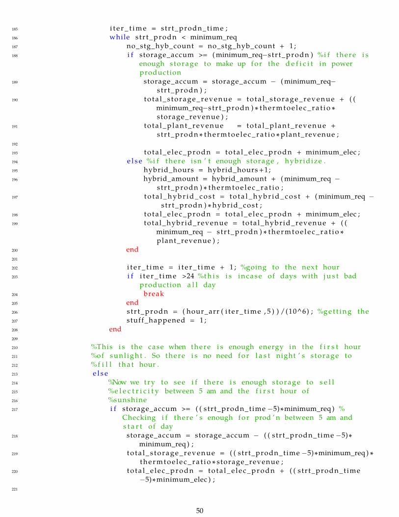
185 i t e r _ t ime = str t_prodn_t ime ;186 while s t r t_prodn < minimum_req187 no_stg_hyb_count = no_stg_hyb_count + 1 ;188 i f storage_accum >= (minimum_req−s t r t_prodn ) %i f there i s

enough storage to make up for the d e f i c i t in powerproduction

189 storage_accum = storage_accum − (minimum_req−s t r t_prodn ) ;

190 to ta l_s torage_revenue = to ta l_s torage_revenue + ( (minimum_req−s t r t_prodn ) ∗ the rmtoe l e c_ ra t i o ∗storage_revenue ) ;

191 to ta l_p lan t_revenue = to ta l_p lan t_revenue +str t_prodn ∗ the rmtoe l e c_ ra t i o ∗plant_revenue ;

192

193 to ta l_e l ec_prodn = to ta l_e lec_prodn + minimum_elec ;194 e l s e %i f there isn ’ t enough storage , hybr idize .195 hybrid_hours = hybrid_hours +1;196 hybrid_amount = hybrid_amount + (minimum_req −

s t r t_prodn ) ∗ the rmtoe l e c_ ra t i o ;197 t o t a l _hybr id_cos t = to t a l _hybr id_cos t + (minimum_req −

s t r t_prodn ) ∗ hybrid_cost ;198 to ta l_e l ec_prodn = to ta l_e lec_prodn + minimum_elec ;199 to ta l_hybr id_revenue = tota l_hybr id_revenue + ( (

minimum_req − s t r t_prodn ) ∗ the rmtoe l e c_ ra t i o ∗plant_revenue ) ;

200 end201

202 i t e r _ t ime = i t e r _ t ime + 1 ; %going to the next hour203 i f i t e r _ t ime >24 %th i s i s incase of days with j u s t bad

production a l l day204 break205 end206 s t r t_prodn = ( hour_arr ( i t e r_ t ime , 5 ) ) /(10^6) ; %ge t t ing the207 stuff_happened = 1 ;208 end209

210 %This i s the case when there i s enough energy in the f i r s t hour211 %of sunl igh t . So there i s no need for l a s t night ’ s s torage to212 %f i l l tha t hour .213 e l s e214 %Now we try to see i f there i s enough storage to s e l l215 %e l e c t r i c i t y between 5 am and the f i r s t hour of216 %sunshine217 i f storage_accum >= ( ( str t_prodn_time −5)∗minimum_req ) %

Checking i f there ’ s enough for prod ’ n between 5 am ands t a r t of day

218 storage_accum = storage_accum − ( ( s tr t_prodn_time −5)∗minimum_req ) ;

219 to ta l_s torage_revenue = ( ( str t_prodn_time −5)∗minimum_req ) ∗the rmtoe l e c_ ra t i o ∗ storage_revenue ;

220 to ta l_e l ec_prodn = to ta l_e lec_prodn + ( ( s tr t_prodn_t ime−5)∗minimum_elec ) ;

221

50

222 e l s e i f storage_accum >= ( ( str t_prodn_time −6)∗minimum_req )%Checking i f there ’ s enough for prod ’ n between 6 am ands t a r t of day

223 storage_accum = storage_accum − ( ( s tr t_prodn_time −6)∗minimum_req ) ;

224 to ta l_s torage_revenue = ( ( str t_prodn_time −6)∗minimum_req ) ∗the rmtoe l e c_ ra t i o ∗ storage_revenue ;

225 to ta l_e l ec_prodn = to ta l_e lec_prodn + ( ( s tr t_prodn_t ime−6)∗minimum_elec ) ;

226

227 e l s e i f storage_accum >= ( ( str t_prodn_time −7)∗minimum_req )%Checking i f there ’ s enough for prod ’ n between 7 am ands t a r t of day

228 storage_accum = storage_accum − ( ( s tr t_prodn_time −7)∗minimum_req ) ;

229 to ta l_s torage_revenue = ( ( str t_prodn_time −7)∗minimum_req ) ∗the rmtoe l e c_ ra t i o ∗ storage_revenue ;

230 to ta l_e l ec_prodn = to ta l_e lec_prodn + ( ( s tr t_prodn_t ime−7)∗minimum_elec ) ;

231 e l s e232 %don ’ t do anything , keep tha t s torage accumulated for

l a t e r233 end234 end235

236 %Now we s t a r t i t e r a t i n g through each hour in the day , accumulatings torage or suplying i t

237 %Also keep in mind to not get excess238

239 %The f i r s t case i s i f in tha t day , there wasn ’ t enough240 %production in the morning and tha t was adjusted for using241 %storage .242 i f stuff_happened == 1243 %i t e r a t i n g through the r e s t of the day s t a r t i n g from where244 %we l e f t o f f l a s t time245 f o r each_hour = ( i t e r _ t ime ) : length ( hour_arr )246 time_hour = hour_arr ( each_hour , 4 ) ;247 power_hour = ( hour_arr ( each_hour , 5 ) ) /(10^6) ;248

249 i f power_hour > max_heat250 power_hour = max_heat ;251 end252

253 %Only enter ing in tha t period when we’ re ge t t ing money fori t

254 i f each_hour >=5 && each_hour <= 22255 i f each_hour >=17 && each_hour <=21256 alpha = 1 . 4 9 7 ;257 e l s e i f each_hour == 22258 alpha = 1 ;259 e l s e i f each_hour >= 5 && each_hour <17260 alpha = 1 ;261 e l s e

51

262 alpha = 0 ;263 end264

265 i f power_hour > minimum_req266 storage_accum = storage_accum + ( power_hour −

minimum_req ) ; %Excess thermal power i s s tored267 to ta l_p lan t_revenue = to ta l_p lan t_revenue +

minimum_elec∗ alpha ∗plant_revenue ;268 tu rb ine_ le f t _ to_produce = turb ine_capac i ty −

minimum_elec ; %how much the turb ine can s t i l lproduce , given i t produces the minimum amountf i r s t

269 to ta l_e l ec_prodn = to ta l_e lec_prodn + minimum_elec;

270

271 i f s t o rage_s i ze == 0272 s t o r age_ l im i t = 10^6;273 storage_accum = 0 ;274 end275

276 i f storage_accum > s to r age_ l im i t277 s torage_excess = storage_accum − s t o r age_ l im i t

; %how much "waste " heat i s ava i l ab l e278 to ta l_was te = ( s torage_excess ∗

the rmtoe l e c_ ra t i o )− tu rb ine_ le f t _ to_produce; %how much of the "waste " heat w i l l not beharnessed by the turb ine

279

280

281 i f to ta l_was te >= 0 %in the case where theturb ine i s not able to harness a l l thewaste heat/ j u s t able to harness i t

282 to ta l_p lan t_revenue = to ta l_p lan t_revenue+ ( turb ine_ le f t_ to_produce ∗plant_revenue ) ;

283 to ta l_e l ec_prodn = to ta l_e lec_prodn +turb ine_ le f t _ to_produce ;

284 storage_waste = storage_waste +to ta l_was te/ the rmtoe l e c_ ra t i o ;

285 e l s e %in the case where the waste heat i s l e s sthan the capac i ty l e f t over in the turb ine

286 to ta l_p lan t_revenue = to ta l_p lan t_revenue+ ( s torage_excess ∗ the rmtoe l e c_ ra t i o ∗plant_revenue ) ;

287 to ta l_e l ec_prodn = to ta l_e lec_prodn + (s torage_excess ∗ the rmtoe l e c_ ra t i o ) ;

288 end289 end290

291 storage_accum = s to r age_ l im i t ;292

293 e l s e i f power_hour <minimum_req && storage_accum > (minimum_req−power_hour )

52

294 storage_accum = storage_accum − (minimum_req−power_hour ) ;

295 to ta l_s torage_revenue = to ta l_s torage_revenue + ( (minimum_req−power_hour ) ∗ storage_revenue ∗the rmtoe l e c_ ra t i o ∗ alpha ) ;

296 to ta l_p lan t_revenue = to ta l_p lan t_revenue +power_hour∗ alpha ∗ the rmtoe l e c_ ra t i o ∗plant_revenue ;

297 to ta l_e l ec_prodn = to ta l_e lec_prodn + minimum_elec;

298 no_stg_hyb_count = no_stg_hyb_count + 1 ;299 e l s e300 hybrid_hours = hybrid_hours +1;301 hybrid_amount = hybrid_amount + (minimum_req −

power_hour ) ∗ the rmtoe l e c_ ra t i o ;302 t o t a l _hybr id_cos t = to t a l _hybr id_cos t + ( (

minimum_req − power_hour ) ∗ hybrid_cost ) ;303 to ta l_e l ec_prodn = to ta l_e lec_prodn + minimum_elec

;304 to ta l_hybr id_revenue = tota l_hybr id_revenue + ( (

minimum_req − power_hour ) ∗ the rmtoe l e c_ ra t i o ∗alpha ∗plant_revenue ) ;

305 no_stg_hyb_count = no_stg_hyb_count + 1 ;306 end307 end308 end309 %s t a r t the i t e r a t i o n from tha t time where i t e r a t i o n

stopped310 e l s e311 f o r each_hour = 1 : length ( hour_arr )312 time_hour = hour_arr ( each_hour , 4 ) ;313 power_hour = ( hour_arr ( each_hour , 5 ) ) /(10^6) ;314

315 i f power_hour > max_heat316 power_hour = max_heat ;317 end318

319 i f each_hour >=5 && each_hour <= 22320

321 i f each_hour >=17 && each_hour <=21322 alpha = 1 . 4 9 7 ;323 e l s e i f each_hour == 22324 alpha = 1 ;325 e l s e i f each_hour >= 5 && each_hour <17326 alpha = 1 ;327 e l s e328 alpha = 0 ;329 end330

331 %I f there was more power produced than required , i t i ss tored

332 i f power_hour > minimum_req333 storage_accum = storage_accum + ( power_hour −

53

minimum_req ) ; %Excess thermal power i s s tored334 to ta l_p lan t_revenue = to ta l_p lan t_revenue +

minimum_req∗ alpha ∗ the rmtoe l e c_ ra t i o ∗plant_revenue ;

335 tu rb ine_ le f t _ to_produce = turb ine_capac i ty −minimum_elec ; %how much the turb ine can s t i l lproduce , given i t produces the minimum amountf i r s t

336 to ta l_e l ec_prodn = to ta l_e lec_prodn + minimum_elec;

337

338 i f s t o rage_s i ze == 0339 s t o r age_ l im i t = 10^6;340 storage_accum = 0 ;341 end342

343 %i f the amount of s torage exceeds how much the344 %storage l im i t i s345 i f storage_accum > s to r age_ l im i t346 s torage_excess = storage_accum − s t o r age_ l im i t

; %how much "waste " heat i s ava i l ab l e347 to ta l_was te = ( s torage_excess ∗

the rmtoe l e c_ ra t i o )− tu rb ine_ le f t _ to_produce; %how much of the "waste " heat w i l l not beharnessed by the turb ine

348

349 i f to ta l_was te >= 0 %in the case where theturb ine i s not able to harness a l l thewaste heat/ j u s t able to harness i t

350 to ta l_p lan t_revenue = to ta l_p lan t_revenue+ ( turb ine_ le f t_ to_produce ∗plant_revenue ) ;

351 to ta l_e l ec_prodn = to ta l_e lec_prodn +turb ine_ le f t _ to_produce ;

352 storage_waste = storage_waste +to ta l_was te/ the rmtoe l e c_ ra t i o ;

353

354 e l s e %in the case where the waste heat i s l e s sthan the capac i ty l e f t over in the turb ine

355 to ta l_p lan t_revenue = to ta l_p lan t_revenue+ ( s torage_excess ∗ the rmtoe l e c_ ra t i o ∗plant_revenue ) ;

356 to ta l_e l ec_prodn = to ta l_e lec_prodn + (s torage_excess ∗ the rmtoe l e c_ ra t i o ) ;

357 end358 storage_accum = s to r age_ l im i t ;359 end360

361 e l s e i f power_hour <minimum_req && storage_accum > (minimum_req−power_hour )

362 storage_accum = storage_accum − (minimum_req−power_hour ) ;

363 to ta l_s torage_revenue = to ta l_s torage_revenue + ( (

54

minimum_req−power_hour ) ∗ the rmtoe l e c_ ra t i o ∗storage_revenue ∗ alpha ) ;

364 to ta l_p lan t_revenue = to ta l_p lan t_revenue +power_hour∗ alpha ∗ the rmtoe l e c_ ra t i o ∗plant_revenue ;

365 to ta l_e l ec_prodn = to ta l_e lec_prodn + minimum_elec;

366 no_stg_hyb_count = no_stg_hyb_count + 1 ;367 e l s e368 hybrid_hours = hybrid_hours + 1 ;369 hybrid_amount = hybrid_amount + (minimum_req −

power_hour ) ∗ the rmtoe l e c_ ra t i o ;370 t o t a l _hybr id_cos t = to t a l _hybr id_cos t + ( (

minimum_req − power_hour ) ∗ hybrid_cost ) ;371 to ta l_e l ec_prodn = to ta l_e lec_prodn + minimum_elec

;372 to ta l_hybr id_revenue = tota l_hybr id_revenue + ( (

minimum_req − power_hour ) ∗ the rmtoe l e c_ ra t i o ∗alpha ∗plant_revenue ) ;

373 no_stg_hyb_count = no_stg_hyb_count + 1 ;374 end375 end376 end377 end378 end379

380 to ta l_revenue = to ta l_p lan t_revenue+to ta l_s torage_revenue ;381

382 i f tu rb ine_capac i ty == 150 && s to rage_s i ze == 1383 date_s tore ( each_day , : ) = hour_arr ( 1 , 1 : 3 ) ; %c rea t ing the f i r s t

three columns of year , month and day384 end385

386 e l e c _ s t o r e ( each_day , column_count ) = to ta l_e l ec_prodn ;387 master_s tore ( each_day , column_count ) = to ta l_revenue ;388 hybr id_s tore ( each_day , column_count ) = ( hybrid_hours ) ; %Average MW of

hybr id iza t ion required in the day389 hybr id_cos t_s tore ( each_day , column_count ) = to t a l _hybr id_cos t ;390 hybrid_revenue_store ( each_day , column_count ) = tota l_hybr id_revenue ;391 s torage_waste_s tore ( each_day , column_count ) = storage_waste ;392 no_stg_hyb_store ( each_day , column_count ) = no_stg_hyb_count ;393

394 to ta l_s torage_revenue = 0 ;395 t o t a l _hybr id_cos t = 0 ;396 to ta l_p lan t_revenue = 0 ;397 to ta l_revenue = 0 ;398 storage_waste = 0 ;399 hybrid_amount = 0 ;400 hybrid_hours = 0 ;401 to ta l_e l ec_prodn = 0 ;402 to ta l_hybr id_revenue = 0 ;403 no_stg_hyb_count = 0 ;404 end

55

405 end406 end407 f i na l _hybr id_ s to r e = [ date_s tore , hybr id_s tore ] ;408 f i na l _hyb r id_co s t _ s t o r e = [ date_s tore , hybr id_cos t_s tore ] ;409 f i n a l _ s t o r e = [ date_s tore , master_s tore ] ;410 f i n a l _ e l e c _ s t o r e = [ date_s tore , e l e c _ s t o r e ] ;411 f ina l_hybr id_revenue_s tore = [ date_s tore , hybrid_revenue_store ] ;412 f i na l _ s to rage_was t e_ s to r e = [ date_s tore , s torage_waste_s tore ] ;413 f i na l _ s tg_hyb_s to r e = [ date_s tore , no_stg_hyb_store ] ;

56