ì  Metagenome  assembly  –  part  II  C.  Titus  Brown  ctb@msu.edu  

Warnings  

This  talk  contains  forward  looking  statements.    These  forward-­‐looking  statements  can  be  iden@fied  by  terminology  such  as  

“will”,  “expects”,  and  “believes”.  

-­‐-­‐  Safe  Harbor  provisions  of  the  

U.S.  Private  Securi@es  Li@ga@on  Act  

 

“Making  predic@ons  is  difficult,  especially  if  

they’re  about  the  future.”  

-­‐-­‐  AOributed  to  Niels  Bohr  

The  computational  conundrum  

 

 

More  data  =>  beOer.  

 

and  

 

More  data  =>  computa@onally  more  challenging.  

Reads vs edges (memory) in de Bruijn graphs

Conway T C , Bromage A J Bioinformatics 2011;27:479-486

© The Author 2011. Published by Oxford University Press. All rights reserved. For Permissions, please email: journals.permissions@oup.com

2.  Big  data  sets  require  big  machines  

For  even  rela@vely  small  data  sets,  metagenomic  assemblers  scale  poorly.  

Memory  usage  ~  “real”  varia@on  +  number  of  errors  

Number  of  errors  ~  size  of  data  set  

Size  of  data  set  ==  big!!  

 

(Es@mated  6  weeks  x  3  TB  of  RAM  to  do  300gb  soil  sample,  with  a  slightly  modified  conven@onal  assembler.)  

GCGTCAGGTAGGAGACCGCCGCCATGGCGACGATG

GCGTCAGGTAGGAGACCACCGTCATGGCGACGATG

GCGTCAGGTAGCAGACCACCGCCATGGCGACGATG

GCGTTAGGTAGGAGACCACCGCCATGGCGACGATG

Soil  is  full  of  uncultured  microbes  

Randy  Jackson  

SAMPLING  LOCATIONS  

Great Prairie sampling design

Reference core

Soil cores: 1 inch diameter 4 inches deep (litter and roots removed)

•  Spatial samples: 16S rRNA, nifH

•  Reference sample sequenced (small unmixed sample)

Reference bulk soil: stored for additional “omics” and metadata

10 M

10 M

1 M

1 M

1 cM

1 cM

0  

200  

400  

600  

800  

1000  

1200  

1400  

1600  

1800  

2000  

100   600   1100   1600   2100   2600   3100   3600   4100   4600   5100   5600   6100   6600   7100   7600   8100  

Iowa  Corn  

Iowa_Na@ve_Prairie  

Kansas  Corn  

Kansas_Na@ve_Prairie  

Wisconsin  Corn  

Wisconsin  Na@ve  Prairie  

Wisconsin  Restored  Prairie  

Wisconsin  Switchgrass  

Number  of  Sequences  

Num

ber  o

f  OTU

s  

Soil  contains  thousands  to  millions  of  species  (“Collector’s  curves”  of  ~species)  

The  set  of  questions  for  soil  -­‐-­‐  discovery  

ì  What’s  there?  

ì  Is  it  really  that  complex  a  community?  

ì  How  “deep”  do  we  need  to  sequence  to  sample  thoroughly  and  systema@cally?  

ì  What  organisms  and  gene  func@ons  are  present,  including  non-­‐canonical  carbon  and  nitrogen  cycling  pathways?    

ì  What  kind  of  organismal  and  func@onal  overlap  is  there  between  different  sites?    (Total  sampling    needed?)  

ì  How  is  ecological  complexity  created  &  maintained?  

ì  How  does  ecological  complexity  respond  to  perturba@on?  

Why  are  we  applying  short-­‐read  sequencing  to  this  problem!?  

ì  Short-­‐read  sampling  is  deep  and  quan(ta(ve.  ì  Sta@s@cal  argument:  your  ability  to  observe  rare  

organisms  –  your  sensi@vity  of  measurement  –  is  directly  related  to  the  number  of  independent  sequences  you  take.  

ì  Longer  reads  (PacBio,  454,  Ion  Torrent)  are  less  informa@ve.  

ì  Majority  of  metagenome  studies  going  forward  will  make  use  of  Illumina.  

ì  BUT  this  kind  of  sequence  is  challenging  to  analyze.  

ì  BUT,  BUT  this  kind  of  sequence  is  necessary  for  high  complexity  environments.  

Challenges  of  short-­‐read  analysis  

ì  Low  signal  for  func@onal  analysis;  no  linkage  at  all.  

ì  High  error  rates.  

ì  Massive  volume.  

ì  Rapidly  changing  technology.  

ì  Several  approaches  but  we  have  seOled  on  assembly.  

Our  “Grand  Challenge”  dataset  

0"

100"

200"

300"

400"

500"

600"

Iowa,"Continuous"corn"

Iowa,"Native"Prairie"

Kansas,"Cultivated"corn"

Kansas,"Native"Prairie"

Wisconsin,"Continuous"corn""

Wisconsin,"Native"Prairie"

Wisconsin,"Restored"Prairie"

Wisconsin,"Switchgrass"

Basepairs(of(Sequencing((Gbp)(

GAII" HiSeq"

Rumen"(Hess"et."al,"2011),"268"Gbp

MetaHIT"(Qin"et."al,"2011),"578"Gbp

NCBI"nr"database,""37"Gbp

Total:""1,846"Gbp"soil"metagenome

Rumen"KSmer"Filtered,"111"Gbp

Approach  1:  Partitioning  

Split  reads  into  “bins”  belonging  to  different  source  species.  

Can  do  this  based  almost  en@rely  on  connec@vity  of  sequences.  

Partitioning  for  scaling  

ì  Can  be  done  in  ~10x  less  memory  than  assembly.  

ì  Par@@on  at  low  k  and  assemble  exactly  at  any  higher  k  (DBG).  

ì  Par@@ons  can  then  be  assembled  independently  ì  Mul@ple  processors  -­‐>  scaling  ì  Mul@ple  k,  coverage  -­‐>  improved  assembly  ì  Mul@ple  assembly  packages  (tailored  to  high  varia@on,  etc.)  

ì  Can  eliminate  small  par@@ons/con@gs  in  the  par@@oning  phase.  

ì  An  incredibly  convenient  approach  enabling  divide  &  conquer  approaches  across  the  board.  

Technical  challenges  met  (and  defeated)  

ì  Novel  data  structure  proper@es  elucidated  via  percola@on  theory  analysis  (Pell  et  al.,  PNAS,  2012)  

ì  Exhaus@ve  in-­‐memory  traversal  of  graphs  containing  5-­‐15  billion  nodes.  

ì  Sequencing  technology  introduces  false  connec@ons  in  graph  (Howe  et  al.,  in  prep.)  

ì  Only  20x  improvement  in  assembly  scaling  L.  

Approach  2:  Digital  normalization  

Species A

Species B

Ratio 10:1Unnecessary data

81%

Suppose  you  have  a  dilu@on  factor  of  A  (10)  to  B(1).    To  get  10x  of  B  you  need  to  get  100x  of  A!    

Overkill!!    

This  100x  will  consume  disk  space  and,  because  of  

errors,  memory.  

(NOVEL)  

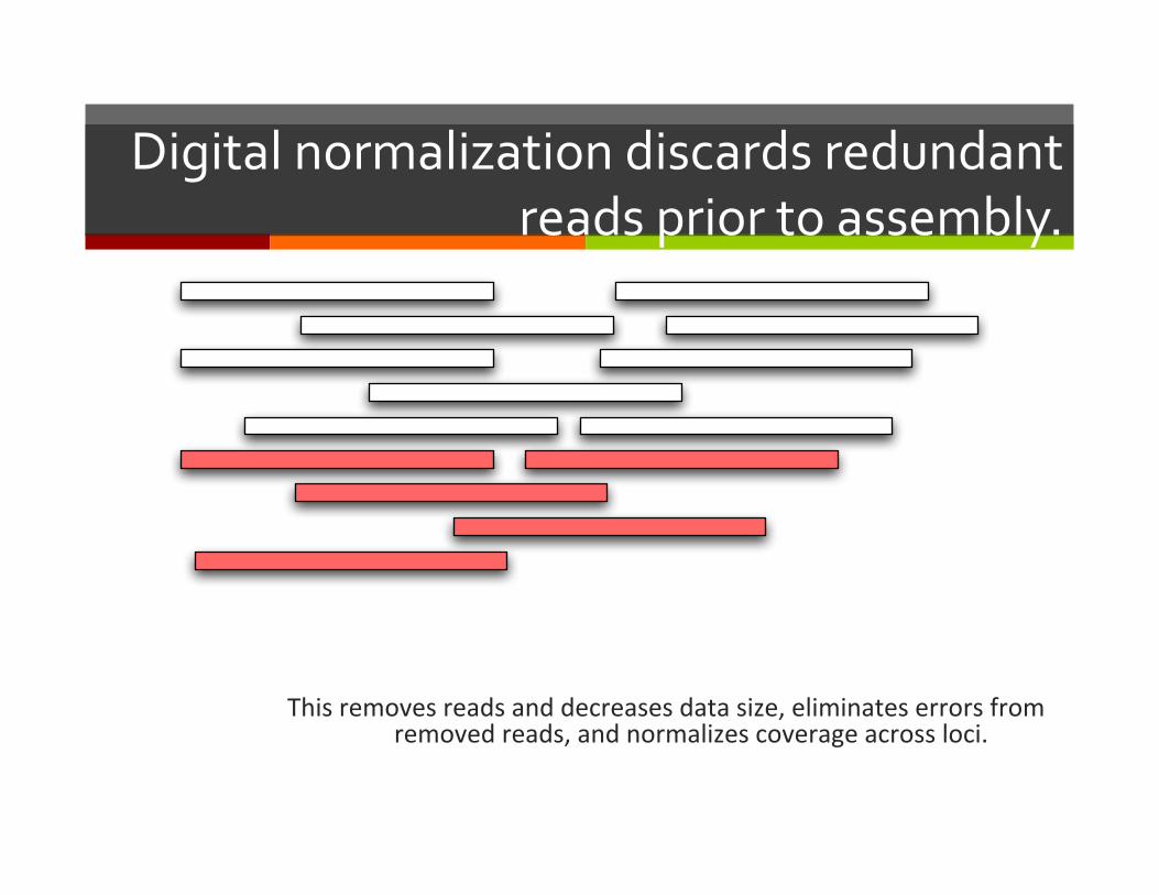
Digital  normalization  discards  redundant  reads  prior  to  assembly.  

This  removes  reads  and  decreases  data  size,  eliminates  errors  from  removed  reads,  and  normalizes  coverage  across  loci.      

Digital  normalization  algorithm  

!

!

for read in dataset:!

!if median_kmer_count(read) < CUTOFF:!

! !update_kmer_counts(read)!

! !save(read)!

!else:!

! !# discard read!

!

! !! Note,  single  pass;  fixed  memory.  

Downsample  based  on  de  Bruijn  graph  structure  (which  can  be  derived  online)  

A. B.

Shotgun  data  is  often  (1)  high  coverage  and  (2)  biased  in  coverage.  

(MD  amplified)  

Digital  normalization  fixes  all  that.  

Normalizes  coverage    Discards  redundancy    Eliminates  majority  of  errors    Scales  assembly  drama@cally.    Assembly  is  98%  iden@cal.  

Digital  normalization  retains  information,  while  discarding  data  and  errors  

Other  key  points  

ì  Virtually  iden@cal  con9g  assembly;  scaffolding  works  but  is  not  yet  cookie-­‐cuOer.  

ì  Digital  normaliza@on  changes  the  way  de  Bruijn  graph  assembly  scales  from  the  size  of  your  data  set  to  the  size  of  the  source  sample.  

ì  Always  lower  memory  than  assembly:  we  never  collect  most  erroneous  k-­‐mers.  

ì  Digital  normaliza@on  can  be  done  once  –  and  then  assembly  parameter  explora@on  can  be  done.  

Quotable  quotes.  

Comment:  “This  looks  like  a  great  soluHon  for  people  who  can’t  afford  real  computers”.  

 

OK,  but:  

 

“Buying  ever  bigger  computers  is  a  great  soluHon  for  people  who  don’t  want  to  think  hard.”  

 

To  be  less  snide:  both  kinds  of  scaling  are  needed,  of  course.      

Why  use  diginorm?  

ì  Use  the  cloud  to  assemble  any  microbial  genomes  incl.  single-­‐cell,  many  eukaryo@c  genomes,  most  mRNAseq,  and  many  metagenomes.  

ì  Seems  to  provide  leverage  on  addressing  many  biological  or  sample  prep  problems  (single-­‐cell  &  genome  amplifica@on  MDA;  metagenome;  heterozygosity).  

ì  And,  well,  the  general  idea  of  locus  specific  graph  analysis  solves  lots  of  things…  

Some  interim  concluding  thoughts  

ì  Digital  normaliza@on-­‐like  approaches  provide  a  path  to  solving  the  majority  of  assembly  scaling  problems,  and  will  enable  assembly  on  current  cloud  compu@ng  hardware.  ì  This  is  not  true  for  highly  diverse  metagenome  environments…  ì  For  soil,  we  es@mate  that  we  need  50  Tbp  /  gram  soil.    Sigh.  

ì  Biologists  and  bioinforma@cians  hate:  ì  Throwing  away  data  ì  Caveats  in  bioinforma@cs  papers  (which  reviewers  like,  note)  

ì  Digital  normaliza@on  also  discards  abundance  informa@on.  

Evaluating  sensitivity  &  specificity  

Digital normalization+ other filters

Partitioning Velvetk from 19-51

minimus2merge

E.  coli  @  10x  +  soil  

98.5%  of  E.  coli  

Example  

Dethlefsen  shotgun  data  set  /  Relman  lab    251  m  reads  /  16gb  FASTQ  gzipped  ~  24  hrs,  <  32  gb  of  RAM  for  full  pipeline  -­‐-­‐  $24  on  Amazon  EC2  

 (reads  =>  final  assembly  +  mapping)    

Assembly  stats:  58,224  con@gs  >  1000  bp  (average  3kb)  

summing  to  190  mb  genomic  ~38  microbial  genomes  worth  of  DNA  

~65%  of  reads  mapped  back  to  assembly  

What  do  we  get  for  soil?  

Total  Assembly   Total  ConHgs   %  Reads  

Assembled  

Predicted  protein  coding  

rplb  genes  

2.5  bill   4.5  mill   19%   5.3  mill    

391    

3.5  bill    

5.9  mill    

22%   6.8  mill    

466    

This  es@mates  number  of  species  ^  

Adina  Howe  

Pu|ng  it  in  perspec@ve:  Total  equivalent  of  ~1200  bacterial  genomes  Human  genome  ~3  billion  bp      

Coverage  of  Assemblies  

Corn            Prairie  

Nearest  reference  in  NCBI    

Most  abundant  con@gs  in  Iowa  corn  metagenome:  Unknown;  alpha/beta  hydrolase  (Streptomyces  sp.  S4);  unknown;  unknown;    hypothe@cal  protein  HMP  (Clostridium  clostridioforme)    Most  abundant  con@gs  in  Iowa  prairie  metagenome:  hypothe@cal  protein  (Rhodanobacter  sp.  2APBS1);  hypothe@cal  protein  (Oryza  sa@va  Japonica);  outer  membrane  adhesin  like  proteiin  (Solitalea  canadensis)  ;  alcohol  dehydrogenase  zinc-­‐binding  domain  protein  (Ktedonobacter  racemifer);  alcohol  dehydrogenase  GroES  domain  protein  (Ktedonobacter  racemifer)              

(Done  with  MEGAN)  

How  many  soil  samples  do  we  need  to  sequence??  

(Cumula@ve)  Adina  Howe  

Overlap  between  Iowa  prairie  &  Iowa  corn  is  significant!  

Extracting  whole  genomes?  

So  far,  we  have  only  assembled  con9gs,  but  not  whole  genomes.  

 Can  en@re  genomes  be  assembled  from  metagenomic  data?    Iverson  et  al.  (2012),  from  

the  Armbrust  lab,  contains  a  technique  for  scaffolding  metagenome  con@gs  into  ~whole  genomes.    YES.    

Perspective:  the  coming  infopocalypse  

ì  Assembling  about  $20k  worth  of  data,  we  can  generate  approximately  700  microbial  genomes  worth  of  data.    (This  is  only  going  to  go  up  in  yield/$$,  note.)  

 

ì  Most  of  these  assembled  genomic  con@gs  

(and  genes)  do  not  belong  to  studied  

organisms.  

ì  What  the  heck  do  they  do??  

More  thoughts  on  assembly  

ì  Illumina  is  the  only  game  in  town  for  sequencing  complex  microbial  popula@ons,  but  dealing  with  the  data  (volume,  errors)  is  tricky.    This  problem  is  being  solved,  by  us  and  others.  

ì  We’re  working  to  make  it  as  close  to  push  buOon  as  possible,  with  objec@vely  argued  parameters  and  tools,  and  methods  for  evalua@ng  new  tools  and  sequencing  types.  

ì  The  community  is  working  on  dealing  with  data  downstream  of  sequencing  &  assembly.  ì  Most  pipelines  were  built  around  454  data  –  long  reads,  and  

rela@vely  few  of  them.  ì  With  Illumina,  we  can  get  both  long  con9gs  and  quan9ta9ve  

informa9on  about  their  abundance.    This  necessitates  changes  to  pipelines  like  MG-­‐RAST  and  HUMANn.  

The  interpretation  challenge  

ì  For  soil,  we  have  generated  approximately  1200  bacterial  genomes  worth  of  assembled  genomic  DNA  from  two  soil  samples.  

ì  The  vast  majority  of  this  genomic  DNA  contains  unknown  genes  with  largely  unknown  func@on.  

ì  Most  annota@ons  of  gene  func@on  &  interac@on  are  from  a  few  phylogene@cally  limited  model  organisms  ì  Est  98%  of  annota@ons  are  computa@onally  inferred:  transferred  

from  model  organisms  to  genomic  sequence,  using  homology.  ì  Can  these  annota@ons  be  transferred?  (Probably  not.)    

This  will  be  the  biggest  sequence  analysis  challenge  of  the  next  50  years.  

Concluding  thoughts  on  “assembly”  

ì  We  can  handle  all  the  data  (modulo  another  year  or  so  of  engineering.)  Bring  it  on!  

ì  Our  approaches  let  us  (&  you)  assemble  preOy  much  anything,  much  more  easily  than  before.    (Single  cell,  microbial  genomes,  transcriptomes,  eukaryo@c  genomes,  metagenomes,  BAC  sequencing…)  

ì  Seriously.    No  more  problemo.    Done.    Finished.    Kaput.  

ì  So  now  what?  ì  Valida@on.  ì  Interpreta@on  and  building  general  tools.  ì  Interpreta@on  relies  on  annota9on…  (Uh  oh.)  

What  are  future  needs?  

ì  High-­‐quality,  medium+  throughput  annota@on  of  genomes?  ì  Extrapola@ng  from  model  organisms  is  both  immensely  

important  and  yet  lacking.  ì  Strong  phylogene@c  sampling  bias  in  exis@ng  annota@ons.  

ì  Synthe@c  biology  for  inves@ga@ng  non-­‐model  organisms?  

(Cleverness  in  experimental  biology  doesn’t  scale  L)  

 

ì  Integra@on  of  microbiology,  community  ecology/evolu@on  modeling,  and  data  analysis.    

Replication  fu  

ì  In  December  2011,  I  met  Wes  McKinney  on  a  train  and  he  convinced  me  that  I  should  look  at  IPython  Notebook.  

ì  This  is  an  interac9ve  Web  notebook  for  data  analysis…  

ì  Hey,  neat!    We  can  use  this  for  replica@on!  ì  All  of  our  figures  can  be  regenerated  from  scratch,  on  an  EC2  

instance,  using  a  Makefile  (data  pipeline)  and  IPython  Notebook  (figure  genera@on).  

ì  Everything  is  version  controlled.  ì  Honestly  not  much  work,  and  will  be  less  the  next  @me.  

So…  how’d  that  go?  

ì  People  who  already  cared  thought  it  was  ni}y.  

hOp://ivory.idyll.org/blog/replica@on-­‐i.html  

ì  Almost  nobody  else  cares  ;(  ì  Presub  enquiry  to  editor:  “Be  sure  that  your  paper  can  be  reproduced.”    Uh,  

please  read  my  leOer  to  the  end?  ì  “Could  you  improve  your  Makefile?  I  want  to  reimplement  diginorm  in  another  

language  and  reuse  your  pipeline,  but  your  Makefile  is  a  mess.”  

ì  Incredibly  useful,  nonetheless.  Already  part  of  undergraduate  and  graduate  training  in  my  lab;  helping  us  and  others  with  next  parpes;  etc.  etc.  etc.  

 

Life  is  way  too  short  to  waste  on  unnecessarily  replicaHng  your  own  workflows,  much  less  other  people’s.  

Acknowledgements  

Lab  members  involved  Collaborators  

ì  Adina  Howe  (w/Tiedje)  ì  Jason  Pell  ì  Arend  Hintze  ì  Rosangela  Canino-­‐Koning  ì  Qingpeng  Zhang  ì  Elijah  Lowe  ì  Likit  Preeyanon  ì  Jiarong  Guo  ì  Tim  Brom  ì  Kanchan  Pavangadkar  ì  Eric  McDonald  

ì  Jim  Tiedje,  MSU  

ì  Billie  Swalla,  UW  

ì  Janet  Jansson,  LBNL  

ì  Susannah  Tringe,  JGI  

Funding  

USDA  NIFA;  NSF  IOS;  BEACON.  

ì  Current  research  in  my  lab  Solving  the  rest  of  your  problems  J  

Preliminary  func@onal  analysis  

Search  SSU  rRNA  gene  in  Illumina  data  

1.  Randomly  sequencing  about  100bp  long  DNA  in  microbial  genomes;  

2.  Everything  is  sequenced;    

3.  Not  limited  by  primers  or  PCR  bias;  

4.  Data  mining  is  the  challenge;  

10^3  

10^6  10^7   10^4  

Reads  #  

SSU  rRNA  Gene  length  

Expected  SSU  RNA  gene  fragments  

Genome  length  

Classification:  Pyrotag  vs  shotgun  

RDP-­‐pyrotag-­‐SSU  

silva-­‐pyrotag-­‐SSU  

silva-­‐shotgun-­‐SSU  

Primers  used  in    454  Titanium  sequencing  of  SSU  rRNA  gene,  using  E.coli  as  an  example.  Consensus  sequences  of  the  primer  region  from  Illumina  reads  suggest  1)  searching  method  is  good  and    2)primer  bias  is  minimal  at  the  current  E-­‐value  cutoff.  

Start:907 End:1402

Forward

Reverse

1542 bp

Sequence logo of short reads at forward primer region:

AAACTYAAAKGAATTGACGG Current forward primer

GYACACACCGCCCGT Current reverse primer (reverse complement)

Sequence logo of short reads at reverse primer region:

CowRumen  –  JGI  16s  primer  mismatches  

postion! A T C G Total 1G! 0.001 0.001 0.002 0.996 12154 2T! 0.002 0.983 0.003 0.012 12169 3G! 0.001 0.001 0.002 0.995 12166 4C! 0.001 0.001 0.996 0.002 12143 5C! 0.003 0.001 0.994 0.002 12183 6A! 0.986 0 0.008 0.005 12209 7G! 0.001 0.001 0.002 0.996 12189 8C! 0.001 0.001 0.996 0.002 12198 9A! 0.978 0.001 0.017 0.004 12230

10G! 0.001 0 0.002 0.997 12231 11C! 0.001 0.001 0.996 0.002 12198 12C! 0.002 0.001 0.994 0.003 12185 13G! 0 0 0.002 0.997 12190 14C! 0.001 0.001 0.995 0.003 12195 15G! 0.001 0.001 0 0.998 12213 16G! 0.001 0.001 0 0.998 12206 17T! 0.002 0.974 0.003 0.021 12171 18A! 0.99 0.001 0.006 0.003 12150 19A! 0.995 0.001 0.002 0.002 12106

Running  HMMs  over  de  Bruijn  graphs  (=>  cross  validation)  

ì  hmmgs:  Assemble  based  on  good-­‐scoring  HMM  paths  through  the  graph.  

ì  Independent  of  other  assemblers;  very  sensi@ve,  specific.  

ì  95%  of  hmmgs  rplB  domains  are  present  in  our  par@@oned  assemblies.  

Jordan  Fish,  Qiong  Wang,  and  Jim  Cole  (RDP)  

Streaming  error  correction.  

Does read come from a high-

coverage locus?

Error-correct low-abundance k-mers in

read.

Add read to graph and save for later.

All reads Yes!

No!

First pass

Does read come from a now high-coverage locus?

Error-correct low-abundance k-mers in

read.

Leave unchanged.

Only saved reads

Yes!

No!

Second pass

We  can  do  error  trimming  of  genomic,  MDA,  transcriptomic,  metagenomic  data  in  <  2  passes,  fixed  memory.  

We  have  just  submiOed  a  proposal  to  adapt  Euler  or  Quake-­‐like  error  correc@on  (e.g.  spectral  alignment  problem)  to  this  

framework.  

Side  note:  error  correction  is  the  biggest  “data”  problem  left  in  

sequencing.  

A. B.

XXX

X

XX

X

X

XX

X

C.

XX

X X

XX

Both  for  mapping  &  assembly.  

End:1402

Consensus of short reads at reverse primer region:

é Figure. Primers used in 454 Titanium sequencing of 16S rRNA gene, using E.coli as an example. Consensus sequences of the primer region from Illumina reads suggest primer bias is minimal at the current E-value cutoff.

Start:907 Forward

1542 bp

Consensus of short reads at forward primer region:

AAACTYAAAKGAATTGACGG Current forward primer

Supplemental:  abundance  filtering  is  very  lossy.  

0.0   20.0   40.0   60.0   80.0   100.0  

Total  

3.8x  par@@on  

8.2x  par@@on  

Largest  par@@on  

Percentage  lost  

Percent  loss  from  abundance  filtering    (all  >=  2)  

con@gs  

bp  

11

Velvet Assembler

Coverage of

Unfiltered by

Filtered Assembly

Coverage of

Normalized Filtered by

Unfiltered Assembly

Coverage of

Reference Genes

by Unfiltered

Coverage of

Reference Genes by

Filtered

Unfiltered Assembly Statitics

(No. of Contigs/Assembly

Length(bp)/Max Contig Size (bp)

Normalized Assembly Statitics

(No. of Contigs/Assembly

Length(bp)/Max Contig Size (bp)

Unfiltered Assembly

Requirements (Memory,

GB / Time (hours)

Small Soil 74.5% 98.6% - - 25,470 / 16,269,879 / 118,753 17,636 / 10,578,908 / 13,246 5 / 4Medium Soil 75.4% 98.1% - - 113,613 / 81,660,678 / 57,856 79,654 / 54,424,264 / 23,663 18 / 21Large Soil 50.8% 86.3% - - 554,825 / 306,899,884 / 41,217 290,018 / 159,960,062 / 41,423 33 / 12*Rumen 75.1% 98.3% 17.2% 14.6% 92,044 / 74,813,072 / 182,003 72,705 / 49,518,627 / 34,683 11 / 14Human Gut 79.5% 88.5% - - 543,331 / 234,686,983 / 85,596 203,299 / 181,934,800 / 145,740 76 / 8*Simulated 84.6% 98.3% 4.5% 3.9% 11,204 / 6,506,248 / 5,151 9,859 / 5,463,067 / 6,605 < 1 / < 1

!Meta-IDBA Assembler

Coverage of

Unfiltered by

Filtered Assembly

Coverage of

Normalized Filtered by

Unfiltered Assembly

Coverage of

Reference Genes

by Unfiltered

Coverage of

Reference Genes by

Filtered

Unfiltered Assembly Statitics

(No. of Contigs/Assembly

Length(bp)/Max Contig Size (bp)

Normalized Assembly Statitics

(No. of Contigs/Assembly

Length(bp)/Max Contig Size (bp)

Unfiltered Assembly

Requirements (Memory,

GB / Time (hours)

Small Soil 75.6% 93.9% - - 15,739 / 9,133,564 / 37,738 12,513 / 7,012,036 / 17,048 < 1 / < 1Medium Soil 67.5% 94.5% - - 76,269 / 45,844,975 / 37,738 52,978 / 30,040,031 / 18,882 2 / 2Large Soil N/A N/A - - N/A 395,122 / 228,857,098 / 37,738 > 116 / incompleteRumen 70.4% 94.4% 15.5% 13.0% 60,330 / 47,984,619 / 54,407 48,940 / 33,276,502 / 22,083 12 / 3Human Gut 74.0% 96.5% - - 173,432 / 211,067,996 / 106,503 132,614 / 142,139,101 / 85,539 58 / 15Simulated 86.5% 93.4% 3.8% 3.5% 8,707 / 4,698,575 / 5,113 7,726 / 4,078,947 / 3,845 < 1 / <1

SOAPdenovo Assembler

Coverage of

Unfiltered by

Filtered Assembly

Coverage of

Normalized Filtered by

Unfiltered Assembly

Coverage of

Reference Genes

by Unfiltered

Coverage of

Reference Genes by

Filtered

Unfiltered Assembly Statitics

(No. of Contigs/Assembly

Length(bp)/Max Contig Size (bp)

Normalized Assembly Statitics

(No. of Contigs/Assembly

Length(bp)/Max Contig Size (bp)

Unfiltered Assembly

Requirements (Memory,

GB / Time (hours)

Small Soil 86.6% 95.8% - - 14,275 / 7,100,052 / 37,720 12,801 / 6,343,110 / 13,246 3 / < 1Medium Soil 82.2% 95.7% - - 66,640 / 33,321,411 / 28,695 56,023 / 27,880,293 / 15,721 10 / < 1Large Soil 78.7% 94.2% - - 412,059 / 215,614,765 / 32,514 334,319 / 171,718,154 / 41,423 48 / 11Rumen 84.7% 97.3% 14.7% 13.4% 62,896 / 40,792,029 / 22,875 55,975 / 34,540,861 / 19,044 5 / < 1Human Gut 84.9% 98.5% - - 190,963 / 171,502,574 / 57,803 161,795 / 139,686,630 / 56,034 35 / 5Simulated 93.2% 96.1% 2.5% 2.4% 6,322 / 2,940,509 / 3,786 6,029 / 2,821,631 / 3,764 < 1 / < 1

Table 2. Comparison of unfiltered and filtered assemblies of various metagenome lumps using Velvet,SOAPdenovo, and Meta-IDBA assemblers. Assemblies were aligned to each other, and coverage wasestimated (columns 1-2). Simulated and rumen assemblies were aligned to available referencegenes/genomes (columns 3-4). Total number of contigs, assembly length, and maximum contig size wasestimated for each assembly, as well as memory and time requirements of unfiltered assembly (columnes5-7). Filtered assemblies required less than 2 GB of memory. Velvet assemblies of the unfiltered humangut and large soil datasets (marked as *) could only be completed with K=33 due to computationallimitations. The Meta-IDBA assembly of the large soil metagenome could not be completed in less than100 GB.

Number of Hits to Unique Genes in 112 Reference Genomes

ABC transporter-like protein 306Methyl-accepting chemotaxis sensory transducer 210ABC transporter 173Elongation factor Tu 94Chemotaxis sensory transducer 51ABC transporter ATP-binding protein 44Diguanylate cyclase/phosphodiesterase 36ATPase 36S-adenosyl-L-homocysteine hydrolase 36Adensylhomocysteine and downstream NAD binding 36Ketol-acid reductoisomerase 34S-adenosylmethionine synthetase 34Elongation factor G 34ABC transporter ATPase 33

Table 3. Annotation of highly-connecting sequences from the simulated metagenome with most hits toconserved genes within the 112 reference genomes [8].

Comparing  assemblers  

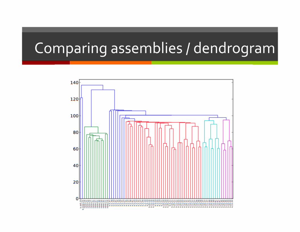
Comparing  assemblies  /  dendrogram  

Integrating  modeling  into  data  analysis?