Cultural Norms and Tenure

Choice? Investigating the High

Homeownership Rate in Taiwan

Huei-chung LuDepartment of Economics, Fu-Jen Catholic University

Mingshen ChenDepartment of Finance,

National Taiwan University

Figure 1. Trends for Homeownership Rates in Taiwan: 1976-2002

60

65

70

75

80

85

90

95

100

1976 1981 1986 1991 1996 2001

Year

(%)

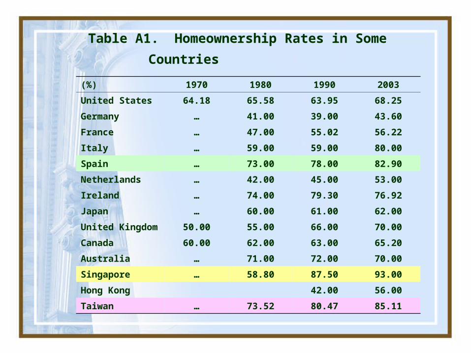
Table A1. Homeownership Rates in Some Countries

(%) 1970 1980 1990 2003

United States 64.18 65.58 63.95 68.25

Germany … 41.00 39.00 43.60

France … 47.00 55.02 56.22

Italy … 59.00 59.00 80.00

Spain … 73.00 78.00 82.90

Netherlands … 42.00 45.00 53.00

Ireland … 74.00 79.30 76.92

Japan … 60.00 61.00 62.00

United Kingdom 50.00 55.00 66.00 70.00

Canada 60.00 62.00 63.00 65.20

Australia … 71.00 72.00 70.00

Singapore … 58.80 87.50 93.00

Hong Kong 42.00 56.00

Taiwan … 73.52 80.47 85.11

I. Introduction

Homeownership: Tenure Choice Model

– Henderson and Ioannides (1983)

Fu (1991); Ioannides and Rosenthal (1994)

– Single Housing Demand: State-Dependent Utility Approach

– Dual Housing Demands: Consumption and Investment

– key factors: wealth, income, property prices, government policy, and conditions of mortgage

Heterogeneity of Homeownership Rates among Ethnic Groups

– Krivo (1995) , Coulson (1999): Hispanic- and Asian-immigrants have the lower homeownership rates.

– Painter, Yang and Yu (2001, 2003, 2004) : Chinese households have the higher homeownership rates.

– Yu (2006): Taiwanese immigrants have the highest homeownership attainment among all ethnic Chinese subgroups.

– Borjas (2002): homeownership gap between native and immigrant households has widened substantially over the past decades .

Table A2. Homeownership Rates by Race and Region in 1990

(%) LA CMSA SF CMSA NY CMSA

White 61.4 59.9 67.3

Asian (all) 57.3 60.7 49.3

Chinese 68.2 69.0 55.4

Filipino 59.3 61.7 51.7

Japanese 62.3 57.7 25.4

Korean 47.9 48.0 38.4

Asian Indian 60.0 59.0 53.9

Other Asian 41.6 37.5 36.9

Source. － Data from Painter, Yang and Yu (2003).

(%) 1980 1990 2000

White 58.2 61.5 66.1

Chinese 61.4 68.2 64.7

Who were born in

Mainland China

Taiwan

Hong Kong/Macau

United States

Other Places

68.7

58.6

55.0

61.0

46.5

70.7

75.0

63.7

67.4

51.4

62.3

71.7

71.4

60.5

58.4

Source. － Data from Yu (2006).

Table A3. Homeownership Rates by Race and Birthplace, Los Angeles CMSA, 1980-2000

Research Motivations:

• Wealth and income are two most important factors in explaining homeownership.

• Countries that have high homeownership rates are Singapore and Taiwan in Asia, Spain in Europe; which are not considered to be the richest countries.

• The richest countries, such as U.S., Japan, and Germany, do not have high homeownership rates

• Chinese has the highest homeownership in the US among all ethnic groups, and Taiwanese has the highest rate among all ethnic Chinese in the US

• Factors other than economical ones? Cultural norms!

Norm Effects and Homeownership

– Assimilation Theory (Gordon, 1964): with learning, sharing and adapting to alternate, different cultures, values and lifestyles, will lead the immigrants to a reduction in ethnic differences and eventually conformity to the mainstream cultural standard.

– Segmented Assimilation (Zhou, 1997; Rumbaut, 2000): some immigrants have experienced their distinctive adaptation processes and may develop a behavioral pattern of perpetual ethnic differences.

– Painter et al. (2003) : Chinese households’ high homeownership rate in the U.S. may be due to factors that are “unmeasured” in the economic data.

– Social Norms Model (Akerlof, 1980): If there is a code of behavior as to how individuals should behave, then those who decide to ignore such norms will endanger their reputations and hence obtain disutilities. An individual’s process to achieve his optimization would produce a peer-group externality that would influence others’ decision.

Table 1. Homeownership by Age, Education and Income in Taiwan: 1986 and 1993

By Ages

Year 30 － 30-39 40-49 50-59 60 ＋

1986 0.8047 0.8062 0.8829 0.9238 0.9135

1993 0.8658 0.8559 0.8806 0.9424 0.9335

By Education Levels

Year EDU1 EDU2 EDU3 EDU4 EDU5  

1986 0.8951 0.8806 0.8353 0.8304 0.8592  

1993 0.9310 0.9115 0.8747 0.8541 0.8941  

By Income Levels  

Year Lowest Second-lowest

MiddleSecond-highest

Highest

1986 0.8122 0.8015 0.8394 0.8887 0.9276

1993 0.8659 0.8347 0.8765 0.9133 0.9470

• Hsueh and Chen (1999) on Taiwan’s high homeownership rates: two possible explanations (but no evidence of proof)– the first is the Chinese culture norm,

– and the second is the long standing subsidy policies employed by the government of Taiwan for the first-time home buyers

This research is organized as follows:

(1)Theoretical model;(2)Data sources and variable definition

s;(3)Econometric model and estimations;(4)Concluding remarks.

II. Theoretical Model

Based on Akerlof’s (1980) setting :

(1)

( , , , , ) ( , , )

( , , ) ( ) .

R C R CC C

R CC

U x h W d d U x h W d d

U x h W d d

: composite consumption

: housing demand; : wealth

: disutility from disobeying the norm

: dummy of not following the norm

: dummy of believing the norm

: homeownership rate of the reference g

C

R

C

x

h W

d

d

roup

: norm effect ( 0)

Assume that all people believe that the norm does exist in the society, thus .

(1’)

− budget constraint for “owning a house” :

− budget constraint for “renting a house” :

1Cd

( , , , , ) ( , , ) ( ) .R RC CU x h W d U x h W d

1

2

,

(1 ) (1 ) ;

C

C C

y x Ph S

W y r S Ph Th

1

2

,

(1 ) .

C

C

y x Rh S

W y r S h

− When owning a house,

− When renting a house,

− If , chooses to be an owner-

occupier; If , chooses to be a

renter.

Given the homeownership rate of peer

group , when becomes larger, the

norm effect will be higher and hence

increase one’s incentive to buy a house.

1 2 ( , , , , , )OV y y P r T

1:Rd

0 :Rd

1 2 ( , , , , , )RV y y R r

O RV VO RV V

III. Data and Variable Definitions

Data Sources : DGBAS (1986, 1993)

– Housing Survey:housing transaction and rental priceshousing characteristics demographic characteristicsnorm proxy

– Survey of Family Income and Expenditure:

household incomedemographic characteristics

More detailed definitions for variables are listed in Appendix.

IV. Econometric Model and Estimated Results

Step 1: The Estimations of Hedonic Prices and Permanent Income

Hedonic housing prices are defined as the implicit prices that can be derived from the housing attributes that affect the prices.

Permanent income is the appropriate income measure used for estimating the housing demand (See Hansen, Formby and Smith, 1996). In addition, household income may be highly correlated with housing demands, cannot be regarded as an exogenous variable in determining tenure choice.

IV. Econometric Model and Estimated Results

(1) Estimations of Hedonic Price and Rent

− Hedonic Theory (Rosen, 1974; Ellickson, 1981) : the implicit prices of attributes or characteristics.

(4)

(5)

1 1

2 2

HPRICE log( ) ,

HRENT log( ) .

i i i i

i i i i

P Z

R Z

Figure 2. Trends for Housing Transaction

Prices of Four Main Cities in Taiwan

0

2

4

6

8

10

1971 1974 1977 1980 1983 1986 1989 1992 1995 1998Year

MillionNT Dollars

Taipei City Taichung City Kaohsiung City Taipei County

Figure 3. Trends for Rental Price Index for Taipei, Kaohsiung and Taiwan

0

20

40

60

80

100

120

1971 1974 1977 1980 1983 1986 1989 1992 1995 1998 2001

Year

Rental Price Index

Taiwan Taipei City Kaohsiung City

Table 3. Estimations for Housing Prices and Rents

VARIABLES

1986 1993

HPRICE HRENT HPRICE HRENT

CONSTANT9.4128**

(89.18)4.6453**

(41.06)10.257**

(94.43)5.7680**

(40.09)

MATERIAL10.4284**

(9.496)-0.0202 (-0.256)

0.5533** (9.049)

0.1403 (1.666)

MATERIAL20.3907**

(10.13)0.0595 (0.962)

0.4033** (6.887)

0.1777* (2.428)

MATERIAL30.0221 (0.577)

0.1081 (1.956)

0.2344** (3.887)

0.1228(1.697)

HTYPE10.5777**

(12.29)0.4500**

(5.112)0.4138**

(11.49)0.4650**

(5.928)

HTYPE20.2247**

(8.499)0.1466**

(2.831)0.1484**

(6.831)0.1259**

(3.002)

HTYPE3-0.3128**

(-15.47)-0.4017**

(-7.679)-0.2136**

(-10.49)-0.3421**

(-6.072)

HUSE-0.2426**

(-12.32)-0.3449**

(-10.17)-0.3078**

(-15.16)-0.4313**

(-12.52)

ROOM1-0.0277**

(-4.749)-0.1316**

(-9.489)-0.0180**

(-2.645)-0.1766**

(-11.29)

ROOM20.0049 (0.636)

0.0071 (0.293)

0.0131 (1.090)

-0.1352** (-4.571)

HAGE-0.0398**

(-33.17)0.0004 (0.225)

-0.0459** (-41.34)

-0.0048** (-2.824)

WATER-0.0219 (-0.213)

-0.0525(-0.607)

0.0601 (0.836)

0.0083 (0.091)

KITCHEN0.3825**(5.584)

0.1515 (1.715)

-0.1500(-1.092)

-0.1706(-1.080)

BATHROOM0.1733**

(2.711)0.1580 (1.900)

0.4826** (3.860)

0.2060 (1.463)

RESTROOM0.1858**

(9.802)0.3281**

(6.290)0.1574**

(7.801)0.2797**

(4.433)

TAIPEI0.2693**

(9.232)0.5683**

(11.69)0.5036**

(18.17)0.7722**

(15.92)

KAOHSIUNG0.0352(1.245)

0.1642** (3.347)

0.0450(1.532)

0.0776(1.474)

TAICHUNG0.4059**

(9.885)0.4784**

(7.847)0.4277**

(10.39)0.3637**

(5.213)

TPECOUNTY-0.0611* (-2.418)

0.3624** (6.899)

0.1522** (6.142)

0.4797** (10.01)

Adjusted R2 0.38 0.33 0.32 0.44

Log-likelihood -9675.9 -1895.4 -11042.9 -1564.7

Sample Size 9,406 1,933 10,544 1,702

(2) The Estimation of Permanent Income

− Goodman (1988), Hoyt and Rosenthal (1990), Rosenthal, Duca and Gabriel (1991):

A permanent income proxy is to regress log of current household income on some socio-economic variables.

(6)3 3LY log( ) .i i i iy W

Table 4. Estimations for Permanent Income

VARIABLES 1986 1993

CONSTANT10.716**(259.2)

11.339**(251.9)

FMSZ0.2085**(37.09)

0.1968**(28.60)

FMSZ2-0.0079**(-16.43)

-0.0079**(-12.34)

MALE0.0846**(7.235)

0.1095**(9.493)

MARRY-0.0115(-1.433)

0.1059**(9.352)

AGE0.0387**(20.24)

0.0506**(27.21)

AGE2-0.0004**(-19.34)

-0.0006**(-30.25)

EDU10.6525**(47.35)

0.5924**(41.15)

EDU20.4888**(35.11)

0.4272**(31.40)

EDU30.3072**(31.94)

0.2353**(22.87)

EDU40.1679**(16.64)

0.0967**(8.766)

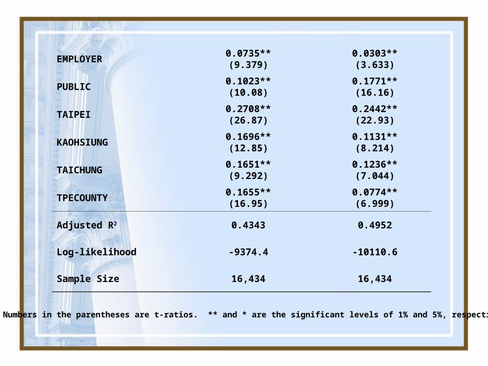
EMPLOYER0.0735**(9.379)

0.0303**(3.633)

PUBLIC0.1023**(10.08)

0.1771**(16.16)

TAIPEI0.2708**(26.87)

0.2442**(22.93)

KAOHSIUNG0.1696**(12.85)

0.1131**(8.214)

TAICHUNG0.1651**(9.292)

0.1236**(7.044)

TPECOUNTY0.1655**(16.95)

0.0774**(6.999)

Adjusted R2 0.4343 0.4952

Log-likelihood -9374.4 -10110.6

Sample Size 16,434 16,434

Note. － Numbers in the parentheses are t-ratios. ** and * are the significant levels of 1% and 5%, respectively .

Step 2: The Estimation of Tenure Choice Model

− We use the setting of the “peer effect” from Evans, Oates and Schwab (1992).

− cultural-norm variable : the community average homeownership rate where the ith household resides.

− We put the imputed income and into a probit model, where

– and our cultural-norm model can be written as:

NORM i

LINC LHPRENT

exp(HPRICE )LHPRENT log log HPRICE HRENT

exp(HRENT )

iii i i

ii

P

R

*1 NORMO R

i i i i i iI V V X

*

*

1 if 0;

0 if 0,

ii

i

II

I

1 1Pr( 1) Pr( NORM ) ( NORM ),i i i i i iI X X

cultural norm effect: the sign and magnitude of .1

LINC

LHPRENT

VARIABLES 1986 1993

CONSTANT-8.3499**(-4.126)

-9.5936**(-5.185)

NORM3.4911**(26.82)

3.3982**(23.89)

0.0869 (0.500)

0.0422(0.290)

0.7949**(25.13)

1.1722**(29.57)

FMSZ0.1244**(4.925)

0.1083**(4.741)

MALE-0.0572(-1.085)

-0.0368(-0.766)

AGE0.0259**(17.04)

0.0197**(11.78)

MARRY-0.1928**(-3.889)

-0.0758(-1.358)

Table 5. Probit Estimations for Cultural-Norm Model

LINC

LHPRENT

EDU10.1570 (1.228)

0.4398**(3.994)

EDU20.3284**(3.061)

0.3363**(3.846)

EDU30.1404* (2.120)

0.2067**(3.789)

EDU40.0017 (0.031)

0.0497(1.003)

PUBLIC0.2013**(3.761)

0.2647**(3.886)

TAIPEI0.0193 (0.290)

0.1024 (1.663)

KAOHSIUNG0.0070 (0.108)

-0.0426(-0.652)

TAICHUNG0.0253 (0.301)

-0.2079* (-2.312)

TPECOUNTY0.1093* (2.005)

0.2709**(5.304)

Log-likelihood -3768.9 -3515.4

Sample Size 11,339 12,246

Correct Prediction 85.92% 88.65%

Summary of results:

(1) NORM has a significantly positive effect on the homeownership rate.

(2) The marginal effect of norms on homeownership is decreased from 1986 (3.4911) to 1993 (3.3982).

(3) has insignificant effect on tenure choice.

(4) has a positive impact on

tenure choice.

LHPRENT

LINC

A positive effect on homeownership• When relative cost of owning house is higher,

people tend to increase the possibility of owning a house – Under the cultural-norm proposition, one has

to possess a property within his life cycle; he would increase the likelihood of owning a house when the housing price increases, expecting that price may go even higher and cost him more to own a property later on.

– Housing investment (or speculation) demand for an individual. When the housing transaction price increases, one would increase property holding, expecting to gain a return when the property price trend is up.

LHPRENT

Step 3: Analysis of Norm Effects by Different subgroups: to see whether norm effects interact with other factors

Clark (2003): the unemployed’s well-being is strongly positively correlated with reference group unemployment (at the regional, partner, or household level), far stronger for men.

Choko and Harris (1990): in North America, homeownership as a cultural norm, but the extent to which people share this norm, varies from place to place.

If norms do exist in a community, the norm effects may be heterogeneous over people with different attributes, such as employment status and locations.

Subgroups 1986 1993

A. Educations:marginal

effectelasticity

sample size

marginal effect

elasticitysample

size

EDU1 0.5286 0.4696 828 0.2382 0.2099 975

EDU2 0.4451 0.3879 758 0.3903 0.3498 1,111

EDU3 0.6657 0.6222 2,120 0.4714 0.4375 2,987

EDU4 0.7154 0.6888 1,683 0.5764 0.5537 2,179

EDU5 0.6213 0.5780 5,950 0.5465 0.5139 4,994

B. Locations:marginal

effectelasticity

sample size

marginal effect

elasticitysample

size

TAIPEI 0.8862 0.8389 1,623 0.5980 0.5647 1,723

KAOHSIUNG 0.6828 0.6410 953 0.7336 0.6821 855

TAICHUNG 0.9040 0.8407 448 0.7151 0.6458 388

TPECOUNTY 0.8068 0.7710 1,672 0.6304 0.5977 1,550

OTHERAREA 0.4479 0.4444 6,643 0.3853 0.3623 7,730

Table 6. Norm Effects by Educations, Locations, Ages, Cohorts, and gender

Subgroups 1986 1993

C. Ages:marginal

effectelasticity

sample size

marginal effect

elasticitysample

size

30- 0.9918 0.9980 1,600 0.6680 0.6442 1,211

30-39 0.9971 0.9791 3,406 0.6872 0.6568 3,935

40-49 0.5063 0.4606 2,795 0.4586 0.4265 3,317

50-59 0.3196 0.2840 2,340 0.2367 0.2155 2,107

60+ 0.4438 0.3996 1,198 0.3963 0.3622 1,676

D. Cohorts:marginal

effectelasticity

sample size

marginal effect

elasticitysample

size

1941- 0.3720 0.3326 4,893 0.3064 0.2794 5,062

1942-1951 0.7232 0.6789 3,118 0.6575 0.6263 4,210

1952+ 1.0827 1.0952 3,328 0.6475 0.6231 2,974

E. Gender:marginal

effectelasticity

sample size

marginal effect

elasticitysample

size

Male 0.5961 0.5524 9,977 0.4543 0.4229 10,208

Female 1.0302 0.9811 1,362 0.6728 0.6363 2,038

F. All Samples:marginal

effectelasticity

sample size

marginal effect

elasticitysample

size

Total 0.6447 0.5991 11,339 0.4923 0.4594 12,246

(1)Education Levels:

The highest marginal norm effect is EDU4, rather than EDU1 or EDU5.

No matter what the education level is, the marginal effects of norms on homeownership subside after the real estate price hike in 1993.

EDU1 tend to have the least bearing with norms during the real estate price hikes, which the marginal effect is hugely reduced from 0.5286 in 1986 to 0.2382 in 1993.

(2) Locations:

Norm effect is the highest in TAICHUNG, and the lowest in OTHERAREA.

Income level is not a cause to different norms effect among all regions.

Norm effects become weaker in most areas of Taiwan in 1993, except for Kaohsiung.

(3) Ages and Cohorts:

Those family heads with age of 30-39 have the highest norm effects, whenever in 1986 or 1993.

“Birth year” is not a key factor since the highest norm effect is those cohorts with 1952+ in 1986, while the highest one is the cohorts with 1942-1951 in 1993.

The impacts of cultural norms on homeownership may be not caused by the

birth year, but the age of a family head.

(4) Gender:

• The gender of a family head has a significantly different impact on the cultural-norm effect on tenure choice.

• The female family head usually are more attached to the cultural-norm effect on their homeownership

V. Concluding Remarks

(1) We use the “cultural norms” to explain Taiwan’s high homeownership rate.

(2) Our empirical evidence shows that Taiwanese residents are heavily influenced by “cultural norms” in their tenure choices.

(3) Family heads with relatively low education backgrounds are more affected by the cultural norms in their tenure choices

(4) Younger family heads’ are more attached to this “cultural norm effect,” and have a higher homeownership rate than that predicted by the theory of life-cycle consumption.

(5) Norm effects are lessened when real estate prices become higher.