data acquisition methods for discrete event...
TRANSCRIPT

Department of Product and Production Development CHALMERS UNIVERSITY OF TECHNOLOGY Gothenburg, Sweden 2014
Data Acquisition Methods for Discrete Event Simulation
A Case Study at Volvo Cars Torslanda Master’s thesis in Production Engineering
ALFREDO CARTER RAMIREZ MARIA LUDVIGSSON

Data Acquisition Methods for Discrete Event
Simulation
A Case Study at Volvo Cars Torslanda
ALFREDO CARTER RAMIREZ
MARIA LUDVIGSSON
Department of Product and Production Development
CHALMERS UNIVERSITY OF TECHNOLOGY
Gothenburg, Sweden, 2014

Data Acquisition Methods for Discrete Event Simulation
A Case Study at Volvo Cars Torslanda
ALFREDO CARTER RAMIREZ
MARIA LUDVIGSSON
© ALFREDO CARTER RAMIREZ & MARIA LUDVIGSSON, 2014.
Department of Product and Production Development
Chalmers University of Technology
SE-412 96 Gothenburg
Sweden
Telephone + 46 (0)31-772 1000
Cover:
The cover picture is a representation of the StreaMod project.
© Volvo Cars Corporation, 2014.
Gothenburg, Sweden 2014

i
Acknowledgement The thesis work could not have been done without the support and help from people in different
departments at Volvo Cars Torslanda, therefore the authors would like to thank everyone who
contributed with their expertise. Foremost the authors would like to thank Jacob Ruda for his
dedication and support from direct simulation expertise to report revision, and everything in
between, throughout the entire thesis process. Special thanks are also given to Dan Lämkull for his
academic guidance and for allowing the realization of this project under his department.
The authors would like to thank Anders Skoogh, the thesis examiner at the department of Product
and Production Development at Chalmers University of Technology, for his continuous support
throughout, and Maheshwaran Gopalakrishnan for supervising the master thesis. Their guidance and
encouragement has been deeply appreciated. This publication has been produced during Alfredo
Carter's scholarship period at Chalmers University of Technology, thanks to a Swedish Institute
scholarship.
Finally, thank you family and friends, without you the thesis would not have been possible from the
very beginning.

ii

iii
Abstract The following thesis work compiles a comprehensive theoretical review of Discrete Event Simulation
Project methodology, with focus mainly on the Input Data Management process and the
requirements of a study case within the automotive industry. A thorough gap analysis between the
simulation input requirements versus the existing information in the organization was made to
illustrate the shortcomings in information availability and quality. The method to collect input
information for the simulation model has been broken down into: data collection, data processing,
and interfacing. Results are based and discussed upon a case study of a real body shop production
scenario at Volvo Cars, in order to illustrate what information sources were explored, used, and
furthermore what kind and form of data could be extracted from them. Specific solutions to compile
the input data for the simulation study are presented and discussed. Integration potentials with
other existent systems in the company were explored and possibilities on further research are
appointed. Finally, several suggestions towards data collection in the current organization and
modeling automation for the specific production case are discussed. The importance of sufficient
quality of data is pointed out in the conclusion, as the following areas were found lacking in the VCT
case: steering logic documentation, disturbance logging, processing time and transportation
between lines.
Keywords: Input Data Management, Discrete Event Simulation, DES requirements, information
sources in automotive industry.

iv

v
Table of Contents Acknowledgement ................................................................................................................................... i
Abstract .................................................................................................................................................. iii
Table of Contents .................................................................................................................................... v
List of figures ......................................................................................................................................... vii
List of Tables ........................................................................................................................................ viii
Definition of terms ................................................................................................................................. ix
1 Introduction .................................................................................................................................... 1
1.1 Who is the customer ............................................................................................................... 1
1.2 Background ............................................................................................................................. 1
1.3 Problem definition .................................................................................................................. 1
1.4 Purpose and goal .................................................................................................................... 2
1.5 Thesis limitations .................................................................................................................... 2
1.6 Study case: Body shop framing process simulation ................................................................ 2
2 Theory ............................................................................................................................................. 5
2.1 Simulation Project Methodology ............................................................................................ 5
2.2 Input data management ......................................................................................................... 7
2.3 Supporting Tools in Simulation ............................................................................................. 17
2.4 Risk Assessment in Data Input for Simulation ...................................................................... 20
2.5 Design of Experiments .......................................................................................................... 20
3 Methodology ................................................................................................................................. 25
3.1 Input Data Management Methodology ................................................................................ 25
4 Simulation Model .......................................................................................................................... 29
4.1 Empirical Data ....................................................................................................................... 30
4.2 Steering Logic ........................................................................................................................ 30
4.3 Processing times ................................................................................................................... 30
4.4 Disturbances ......................................................................................................................... 31
4.5 Transport ............................................................................................................................... 31
5 Information map at VCT ................................................................................................................ 33
5.1 Input Data Sources ................................................................................................................ 33
5.2 Program Software Sources at VCT ........................................................................................ 35
5.3 Information Sources .............................................................................................................. 36
6 Gap Analysis .................................................................................................................................. 39
6.1 Category A Data: Available.................................................................................................... 39
vi
Gap Analysis ...................................................................................................................................... 39
6.2 Category B Data: Available But Not Collectable ................................................................... 47
Gap Analysis ...................................................................................................................................... 47
6.3 Category C Data: Not Available ............................................................................................. 50
Gap Analysis ...................................................................................................................................... 50
7 Input Data Management at VCT ................................................................................................... 55
7.1 Overview of the available formats ........................................................................................ 55
7.2 CTview ................................................................................................................................... 56
7.3 SUSA ...................................................................................................................................... 56
8 Discussion & Suggestions .............................................................................................................. 59
8.1 Required Simulation Parameters .......................................................................................... 59
8.2 Simulation Model .................................................................................................................. 62
8.3 Information mapping ............................................................................................................ 62
8.4 Suggestions ........................................................................................................................... 62
9 Conclusion ..................................................................................................................................... 65
9.1 Main changes ........................................................................................................................ 65
9.2 General changes .................................................................................................................... 65
9.3 Suggestions for the future .................................................................................................... 66
References ............................................................................................................................................ 67
Appendix A ............................................................................................................................................... I
Appendix B ............................................................................................................................................. III
Appendix C ............................................................................................................................................. IX
Appendix D ............................................................................................................................................. XI

vii
List of figures Figure 1 Process flow of VCT Body Shop ................................................................................................................. 3
Figure 2 Simulation methodology described by Musselman (1994) ....................................................................... 5
Figure 3 Simulation methodology by Banks (1998) ................................................................................................ 6
Figure 4 Input data management methodology by Skoogh and Johansson (2009) ............................................... 9
Figure 5 Input data management methodology by Skoogh and Johansson (2009) ............................................... 9
Figure 6 Statistical distribution parameters in Plant Simulation™ ....................................................................... 14
Figure 7 The packages of the CMSD Information Model (SISO 2010) ................................................................... 16
Figure 8 Data input methodologies A, B, C, and D (Robertson and Perera, 2002). .............................................. 17
(Left) Figure 9 Operation tree Y352 11-541-000 MPF and Respot ........................................................................ 18
(Center) Figure 10 Resource tree st11_54_020_56 .............................................................................................. 18
(Right) Figure 11 Product tree Y352 Body ............................................................................................................ 18
Figure 12 Input data management methodology, Skoogh and Johansson (2008) ............................................... 25
Figure 13 Overview of VCT databases .................................................................................................................. 27
Figure 14 Simulation layout with Sankey Diagram for each line products ........................................................... 29
Figure 15 Information mapping of data and information sources at VCT ............................................................ 33
Figure 16 Body shop production in VCT ................................................................................................................ 34
Figure 17 (Left) Resource tree in Process Designer ............................................................................................... 35
Figure 18 (Right) Resource tree at a deeper node level in Process Designer ........................................................ 35
Figure 19 Simulation export only support until version 9.0 of Plant Simulation ................................................... 36
Figure 20 CTview ................................................................................................................................................... 41
Figure 21 SUSA ...................................................................................................................................................... 42
Figure 22 TAP introduction page overview ........................................................................................................... 43
Figure 23 BEO option overview in TAP .................................................................................................................. 43
Figure 24 PERT diagram from Process Designer .................................................................................................. 44
Figure 25 Resource tree and hierarchy ................................................................................................................. 45
Figure 26 Auto CAD drawing over delimited production body shop area in VCT .................................................. 46
Figure 27 Simulation attributes, which can be setup in instances of Resources in Process Designer™ ............... 49
Figure 28 Simulation attributes which can be setup in Process Objects in Process Designer™ ........................... 49
Figure 29 Simulation attributes found in the Product Object class in Process Designer™ .................................. 50
Figure 30 Gathered data related to buffer places in the EOM transportation system ......................................... 52
Figure 31 Not updated Auto CAD drawing ........................................................................................................... 52
Figure 32 Auto CAD drawing with dedicated transport tracks and added not updated areas ............................. 53
Figure 33 Cycle times after processing data. ........................................................................................................ 56
Figure 34 Collected disturbance data for station 11-51-010 from SUSA .............................................................. 57
Figure 35 Input data sheet in MS Excel for disturbances ...................................................................................... 58
Figure 36 Sand cone model with main priorities displayed bottom-up ................................................................ 65
Figure 37 CTview interface in OEE ........................................................................................................................... I
Figure 38 Processing times in CTview ..................................................................................................................... II
Figure 39 Logged signals in SUSA .......................................................................................................................... III
Figure 41. Access to TATS Script tool. .................................................................................................................... IX
Figure 42. Edited Station identifier and generated file link. ................................................................................... X
Figure 43 TATS Script .............................................................................................................................................. X
Figure 44. Output statistics .................................................................................................................................... XI
Figure 45. Second experiment simulation results .................................................................................................. XI
Figure 46. BSI -LH buffer utilization. ..................................................................................................................... XII
Figure 47. BSI -RH buffer utilization. ..................................................................................................................... XII

viii
List of Tables Table 1 Line description over the study case at VCT ............................................................................... 3
Table 2 Data classification .................................................................................................................... 10
Table 3 Statistical distribution functions in DES .................................................................................... 13
Table 4 Design matrix from Bergman and Klefsjö (2010) ..................................................................... 21
Table 5 Design of experiments example with two samples, directly from Goos and Jones (2011) ...... 23
Table 6 Gap analysis category A data ................................................................................................... 39
Table 7 Gap analysis category B data ................................................................................................... 47
Table 8 Gap analysis category C data ................................................................................................... 50
Table 9 Overview of the data format in the information sources at VCT ............................................. 55

ix
Definition of terms A-factory – Car bodies factory at VCT
AutoCAD™™ – CAD layout program
BIW – Body in white, car body before painting.
BOM – Bill of Material
BOP – Bill of Processes
BSI – Body Side Inner
BSO – Body Side Outer
CBS – Corporate Business System
Chalmers – Chalmers University of Technology
CTView – VCT Webpage application to explore historical information on station times
DES – Discrete Event Simulation
DOE – Design of Experiments
DSS – Decision Support System
EBOM – Engineering Bill of Material
eBOP – electronic Bill of Processes
EOM – Electric Overhead Monorail
eMS –Brand of manufacturing planning database Tecnomatix™
ERP – Enterprise Resource Planning
LH – Left Hand side
Line-54 – The investigated production line at VCT, car body framing process
MBOM – Manufacturing Bill of Material
MDT – Mean Down Time
MES – Manufacturing Execution System
MRP – Manufacturing Resource Planning
MPS – Material Planning System
MTTR – Mean Time To Repair (or just TTR)
MTBF – Mean Time Between Failure (or just TBF)
OEE – Overall Equipment Effectiveness
OEE Portalen – VCT log monitoring system for the Virtual Device at TA
PD – Process Designer™
PDM – Product Data Management system
PLC – Programmable Logic Controller
PLM – Product Lifecycle Management
RH – Right Hand side
SCADA – Supervisory control and data acquisition
StreaMod – Research project: Streamlined Modeling and Decision Support for Fact-based
Production Development
SPC – Statistical Process Control
SUSA – Disturbances log system at TA
TA – Torslanda A-Factory
TAP – Torslanda A-fabrik Produktionstyrning
TATS – TA Terminal Services, monitoring system website for TA
TATS Script – A web script that queries a station at TA for historical logged data in the VD

x
The thesis – The current investigation of this thesis
VBA – Visual Basic Application
VCC – Volvo Cars Corporation
VCT – Volvo Cars Torslanda
VD – Virtual Device, SCADA system at TA
Vinnova – Swedish Governmental Agency for Innovation Systems

1
1 Introduction “Discrete Event Simulation (DES) is one of the most powerful tools for planning, designing and
improving material flows in production” (Skoogh et al., 2012). Productivity solutions, which used to
be tested in a real production environment, can now be tested in the virtual world. From the authors’
perspective resource savings and more accurate investments are two of the positive outcomes from
production simulation modeling. However, the process of building the model can be anything but
straightforward as there is often a lack of stored simulation input data in corporate business systems.
This yields in increased time consumption as the data collection and quality verification often needs
to be completed manually. The thesis investigates this potential improvement further to put light on
essential parameters needed for an automatically created and updated discrete event simulation
model.
1.1 Who is the customer The thesis is made within the field of Production Engineering at Chalmers University of Technology,
also referred to as "Chalmers", as part of the research project "StreaMod" in which several industrial
and academic partners are involved. Specifically the thesis will benefit the Manufacturing
Engineering department of Volvo Cars Corporation at their Torslanda production site in Gothenburg,
Sweden, hereafter referred as "VCT".
1.2 Background VCT currently produce six different car bodies in the same flexible production line. Increased
complexity and reconstructions as well as new model introductions have affected the efficiency of
the production line through the years and invalidated previous research studies. In order to stay
competitive VCT, through the “StreaMod” project, aims to cut the lead time from program start to
delivery of the first unit from 36 to 20 months and reaching an Overall Equipment Effectiveness of
above 85% in their running production. These world-class levels require the use of Virtual
Manufacturing tools to enable production development engineers to have a powerful and responsive
decision support system.
In order to address this industrial need, VCT and Chalmers along with StreaMod partners, have been
granted Vinnova (Swedish Governmental Agency for Innovation Systems) funds to research on the
project StreaMod: “Streamlined Modeling and Decision Support for Fact-based Production
Development”, and the thesis work is considered as an initial step towards the general project goal.
One of the current main problems for StreaMod’s industrial partners is the extensive time-
consumption in simulation project, mainly due to inefficiencies in data management (>30% of project
time) and experimentation. Production development engineers waste a significant amount of time
collecting and processing data to validate simulation models, before they are able to prove concepts
or generate value out of experimentations.
1.3 Problem definition Data collection is a manual and time consuming task, necessary in the process of creating a Discrete
Event Simulation (DES). A task which tend to add distraction in the work of a production simulation
modeler, who end-up spending energy and time collecting input data instead of focusing efforts to

2
generate and validate improvements aimed at the production line. Therefore, the thesis investigates
two research questions that could provide a solution:
RQ1. What are the requirements for input data to generate a simulation model that
addresses a common engineering question?
RQ2. How can a simulation model be integrated to the production data sources to
automate the model creation and update of the required input information?
1.4 Purpose and goal Previous studies have shown that it is possible to automate input data for simulation models but
further research work should be done to investigate which and how specific data from the different
sources at VCT can be used in a Decision Support System (DSS) through a DES study case scenario.
In the thesis, a gap analysis of a specific study case in the current production line at VCT is presented
in order to help clarify availability and quality of the production data. Investigated data will be
directly related to the input requirements for a more efficient future integration to an automatic
simulation model creation and update. It has been decided to take a section of the A-factory as
delimitation of the study case, further information on the line can be found in section 1.6.
Exploration within the scope will be done to find which information sources that are reliable and of
interest for the most frequently asked questions in production, learn how to manage them and how
to integrate a suitable simulation model.
The goal is, through input data management, model generation and a gap analysis, to provide a
foundation with sufficient quality for the future creation of an automatically generated and updated
DES model that can function as pioneer towards the development of the Decision Support System for
production and maintenance engineers within the time period of February to June 2014.
1.5 Thesis limitations The thesis will not include any kind of application or script to extract process and input the data
automatically from the several available databases into the simulation model. The intention of this
project is rather to point out the existence, location and form of the data needed as input for the
simulation case.
1.6 Study case: Body shop framing process simulation As mentioned previously in section 1.4, the area of study is limited to a section of the body shop at
VCT. The intention of building the simulation model is to realize what kind of information is needed
in order to do a capacity study of the production line, and compare the results with reality. The main
process of this selection is Line-54, or Framing Line, where under body, left and right sides, and roof
beam lines converge. The first process station of the Framing Line, station 11-54-020, is considered to
be the heart of the body shop factory due to its complexity and importance concerned the overall
process of the body production. Station 11-54-020 is the actual assembly point for sides, roof, and
under body and is thus considered critical to keep from starvation. For this reason the thesis will
include the lines 51, 52, 56 and 57, producing the complete sides, which have been pointed out as
possible causes to starvation issues. Therefore the simulation model will be limited according to
Table 1.

3
Process name Line Description
Framing 11-54 Main process, 11-54-020 framing station Body Side Outer (BSO) -RH 11-52 Process+ Assembly of BSI + Transport system Body Side Inner (BSI) -RH 11-56 Process + Transport system Body Side Outer (BSO) -LH 11-51 Process + Assembly of BSI + Transport system
Body Side Inner (BSI) -LH 11-57 Process + Transport system Roof Beams 11-54 Simplified representation Under Body 11-43 Simplified representation
Table 1 Line description over the study case at VCT
The production process is similar for the two side lines. The Body Side Inners (BSI) are assembled in
lines 56 and 57 which have dedicated fixtures for each product type, therefore the transport system
must be able to change the fixtures based on order. The BSIs are processed in several stations before
being transferred in the last station from the fixture to a hanger transport system, which serves both
as a buffer and a conveyor. The hanger system is a so-called electric overhead monorail (EOM)
system in the roof. The hanger system moves the BSI to the assembly station (11-51-060 or 11-57-
060) at the Body Side Outer (BSO) line where the BSI is assembled into the correspondent BSO.
At the BSO line the transport fixtures are also product type specific. When the first station starts the
transport system must have the correct carrier type available before entering the actual line with
several processing stations, including the previously mentioned BSI assembly. Finally the BSO is
transported to the Framing Station.
The Roof Beams line is a short process with only a few assembly stations. The under-body line is
complex and will have simplified representation in the thesis. Section 4 Simulation Model, contains
further information about the production system. Figure 1 Process flow of VCT Body Shop, shows the
scope of the simulation project within the enclosed area.
Figure 1 Process flow of VCT Body Shop

4

5
2 Theory The thesis is supported by a literature review in the areas of DES-project methodology, input data
management and quality of data through statistical analyses.
2.1 Simulation Project Methodology A successful simulation project is run according to guidelines. This reduces the risk of failure within
the project and enables a time plan to be kept. Musselman (1994) suggests one approach with eight
guidelines: (1) Problem definition and clear result objectives, (2) Model conceptualization, (3) Data
collection, (4) Build model, (5) Verification and Validation, (6) Analysis, (7) Documentation, and (8)
Implementation, see Figure 2.
Figure 2 Simulation methodology described by Musselman (1994)
The approach is supported by Banks (1998) who divides the steps under twelve similar headlines,
where the logic between the steps is added for a more comprehensive and detailed overview, see
Figure 3. The methodology described by Musselman and Banks is verified to be valid still according to
Williams and Ülgen (2012).
A simulation project should be started with (1) a well-defined problem formulation and (2) setting
clear objectives. Solving objectives out of the project scope is time consuming and does not add value
to the project, thus it is important to listen to the customer and have precise and clear objectives
defined from the very start, Musselman (1994). Focus is kept throughout the project by
communicating information in advance and using shorter and more frequent deliveries. It can also
be advisable to create a reference point by asking the customer to predict the solution. The
conclusions, drawn from the simulation project, can then be clearer to the customer in the end.
The next step of the project is (3) the data collection process. The sample size of collected data
should be around 200-230, Banks (1998) Skoogh and Johansson (2008), Perrica et al. (2008). A
smaller sample size reduces the quality of the input data and makes the analysis less reliable. A larger
sample size has shown to not improve the quality noticeable, Banks (1998). The collected data should
be questioned with source and content, together with stated collection methods. Consideration to
these questions enables an estimation of the data-sensitivity thus increasing the model robustness
with more accurate output. When absolute data cannot be found, educated assumptions can be
made in order for the project to move on, Musselman (1993). A previous Master thesis in the area of
simulation, by Andersson and Danielsson (2013), experienced this situation and the project could
only move forward by making such an educated guess.
1. Problem definition and
objectives
2. Model conceptualization
3. Data collection 4. Build model 5. Verification and Validation
6. Analysis 7.
Documentation 8.
Implementation

6
3. Model conceptualization 4. Data collection
1. Problem formulation
2. Setting of objectives and overall project plan
6. Verified?
5. Model translation
No No
Yes
7. Validated?
9. Production runs and analysis
10. More runs?
11. Documentation and
reporting
No
8. Experimental design
Yes Yes
Yes
No
12. Implementation
Figure 3 Simulation methodology by Banks (1998)

7
Banks (1998) suggests (4) a model conceptualization parallel to the data collection process. From
these two steps the actual model (5) is built continuously. By starting simple and only model basic
functions increases the modelers’ ability to fully understand the system’s structure and operating
rules, Banks (1998). Increasing the complexity and adding on functions to a basic model makes it
easier to understand produced outputs, Musselman (1994). The added detail should be based on
stated objectives where components are only added when impacting decision making or confidence
building, Banks (1998). The building of the model includes input procedures and interfaces, division
of model into smaller logical elements, separation of physical and logical model-elements, clear
documentation in the model, and leaving “hooks” to enable future extensions of the model, Banks
(1998).
Throughout the building of the model the functionality should be assessed continuously by
verification (6) and when acceptable the model should be (7) validated to be an accurate
representation of the real system, Banks (1998). It is important to have an accurate representation to
be able to produce useable experimentation results. Musselman (1994) emphasizes on the
importance of involving customers in this phase as the customer often request changes along the
way of a simulation project. Even a small change may cause great impact on the total system. Thus
customers should take part of change request meetings in order to keep in line with the initial scope
and objectives of the project, in order to keep changes at a minimum or when absolutely necessary.
The experimental design (8) is the preparation step of scenarios which are to be investigated. This
step includes length of simulation run, number of runs, and initialization, Banks (1998). Step (9)
production runs and analysis is connected with step (10) concerning the question if more runs are
needed. First the simulation model is run according to the experimental design and secondly the
results are analyzed to conclude the performance depending on experimental scenario. Questioning
the system output and understanding the model’s limits is typically a part of the analyze phase,
Musselman (1994).
Finally step (11) documentation and reporting is done by the modeler, describing the model and its
functionality. According to Banks (1998) this is an important step for future use of the model by
analysts either for further analysis or creation of new scenarios which demands changes in the
current simulation model. The end of the simulation model project is when sufficient information has
been provided for the customer to make a decision on implementation (12).
2.2 Input data management The collection of data input to simulation modeling projects is stated to be the most time consuming
activity requiring more than 30 percent of total project time according to company studies, Skoogh
and Johansson (2007), Perera and Liyanage (2000). It is also a crucial part to enable accurate
outcome from the simulation model, Robertson and Perera (2002). Therefore it is essential in the
thesis to provide a clear view of the data collection process. This section provides a description of
data classification and different methodologies used today for data collection.
Data collection methodology for input data management 2.2.1
In general companies today do not utilize a standardized method for data collection. This was a
discovery by Skoogh and Johansson (2009) based on industry case studies. From this discovery a
method was developed, see Figure 5, from the definition of input data management as “the entire

8
process of preparing quality assured, and simulation adapted, representations of all relevant input
data parameters for simulation models”.
Data acquisition is addressed in detail by Johansson and Skoogh (2008) by breaking down the data
acquisition step of Banks methodology into a process of input data management. This process can be
defined into three main parts: Data collection, data processing and interfacing.
Data collection 2.2.2
A simulation is built upon the information that is available about the process, the resources and the
material flow. Qualitative and quantitative information can provide the simulation modeler with the
understanding that is needed to correctly represent the system. Qualitative referring to the
descriptions and qualities of the process, whereas quantitative refers to the numerical values that
have been registered about the processes. Nevertheless, for the purpose of the thesis only
quantitative data will be evaluated and further analyzed. It is out of the thesis scope to automate the
creation and update of a model with qualitative data, as stated on RQ2 in section 1.3.
Some typical data sources used in input data management are:
Corporate Business Systems (CBS)
- ERP
- PLM
Project specific data
- Layouts
- Project Documentation
Collected data
- From SCADA
- Time studies
External reference systems
- Suppliers
- Industry databases
The CBS is the combined software systems which gather and manage data within an organization,
Robertson and Perera (2002). Enterprise Resource Planning (ERP) is a typical example of a CBS.
Project specific data is data created within a project for the own purpose of the project. Layouts and
general project documentation are good examples.
Collected data is available data which has been taken directly by measurements in the production,
such as time studies, or from data collection systems within the organization.
External reference systems are information or data which is gathered from external sources.
Examples of these are suppliers, knowledge from line builders in the automotive industry, and
general industry databases for equipment.

9
Compile available data Gather not available data
Create data sheet
Identify and define relevant parameters
Specify accuracy requirements
Identify available data
Choose methods for gathering of not available data
Will all specified
data be found
Validate data representations
Sufficient
representation?
Validated?
Finish final
documentation
Prepare statistical or empirical representation
Yes
Yes
Yes
No
No
No
Figure 4 Input data management methodology by Skoogh and Johansson (2009)

10
The data sources get affected mainly by conditions like size of the organization and technology in the
equipment. In industry it is very common to find the information sources to be spread across the
enterprise (Robertson and Perera, 2002), which makes it difficult to concentrate all the information a
broad simulation project would need. Additionally, the amount of historical information can vary
significantly depending on the matureness of a manufacturing system, whereas it is a planning or
current production stage, engineers might use different purpose applications and systems to extract
information about the scenario to model.
Data classification
Data can be classified in three different groups according to Table 2, Robinson and Bhatia (1995).
Table 2 Data classification
Category Data availability
Category A Available
Category B Not available but collectable
Category C Not available and not collectable
As described in the previous section the first step is to start mapping the data according to simulation
model objectives and organize it in the three groups. The process of arranging available data in
category A is straightforward. Category B data is more complicated where calculations and
assumptions need to be made. Category C data is the data which can be found relevant for
simulation purposes but is not yet collectable, thus not available and not collectable.
Data Processing 2.2.3
Data processing refers to the transformation and analysis of raw data into useful information for the
simulation model (Davenport and Prusak 1998). Skoogh and Johansson (2008) state that the output
of data collection activities is already pre-analyzed data and/or sets of raw data, and that the analysis
effort is considerably larger in samples of data describing variability than in those with only constant
data. According to Robinson (2004) variability in data could be represented using one out of four
options: traces, empirical distributions, bootstrapping, or statistical distributions; where empirical
and statistical distributions are the most typical representations in DES software applications. For this
reason, the data processing step should aim to generate simulation model input parameters which
satisfy a valid representation of the collected data.
Data processing is a time-consuming task according to Skoogh and Johansson (2007), because it
requires knowledge about the quality of both the collected data and the required parameters format
that are needed as input for the simulation model. The user is responsible to validate the result, and
if it is found not significant then more data need to be collected. To address this issue the thesis
refers to the activities required for transforming data into information developed by Davenport and
Prusak (1998):
1. Contextualization Knowledge about what purpose the data were collected for.
2. Categorization Knowledge about units of analysis or key components of the data.

11
3. Correction Removal of errors from the data.
4. Calculation Mathematical calculations or statistical analysis of the data.
5. Condensation Summarizing of the data in a more concise form.
From the simulator point of view it is important to have the best representation of reality in the form
of input parameters for the simulation model. Some simulation software applications include
statistical tools to analyze and extract the parameters for the simulation out of the data sample.
Additional adaptations of the data must be performed previously in order for the statistical tool to
read the sample in the correct units. As mentioned by Robinson (2004), statistical or empirical
distributions are most common because they condense the data set to a convenient size.
Several researchers have agreed on a process on how to go from raw data to statistical distributions.
It has been divided in four steps, Banks, Carson, and Nelson (1996); Pedgen, Shannon, and Sadowski
(1995); Leemis (2004):
1. Evaluating the basic characteristics of the empirical data set.
2. Select distribution families for evaluation.
3. Select the best-fitting parameter values for all chosen distribution families.
4. Determine the “goodness-of-fit” and select the best distribution.
Contextualization and Categorization
In order to start processing the raw data a good starting point would be to replicate Davenport and
Prusak (1998) approach and both contextualize and categorize the data set to know its purpose,
reason for being collected, and characteristics about its form. To help with this task, the data set can
be classified into probabilistic or deterministic, and discrete or continuous:
Deterministic Input Data – Occurrence of data in a predictable manner each time, e.g.
preventative maintenance intervals, conveyor velocities, Chung (2004).
Probabilistic Input Data – A process which does not occur with regularity and does not follow
an exact known behavior, e.g. inter-arrival times, repair times, Chung (2004).
Discrete Data – Can only take certain values, usually a whole number. E.g. number of
products processed before machine breakdown, Chung (2004).
Continuous Data – Can take any value in an observed range, e.g. time between arrivals,
service times, Chung (2004).
Correction: Quality of Data
In the Input Data Management methodology proposed by Skoogh and Johansson (2008), data
accuracy requirements must be established before available data identification or any data collection
is performed. As consequence a gap is generated between the available data and the simulation
requirements, which defines the quality of the collected data. Having poor data availability is the
major reason for pitfalls in input data collection according to Perera and Liyanage (2000). Perrica et
al. (2008), state that the amount of samples that must be taken into consideration to estimate
probability functions should be at least 230. Skoogh and Johansson (2008) agree that this estimation
can be used as a good rule of thumb for most parameters. It has also been proven by Skoogh et al.
(2012) that it is possible to automate the extraction and correction of data in cases where the

12
correction actions are a repetitive task. Nevertheless, when the quality of data is inconsistent at each
collection event it is difficult to automate the data processing and utilize automation tools like the
GDM-Tool proposed by Skoogh et al. (2012), which becomes unfeasible.
Calculation: Statistical analysis
After the first three steps of data collection, quality evaluation, and correction have been done, the
available quantitative samples need to be statistically analyzed and be described through statistical
functions. The use of empirical data in the simulation model should be avoided because it lacks
unobserved data in the system, which is covered by the tails of the statistical functions.
According to Chung (2004) data can be found not only in production data bases or systems, but also
from manufacturing specifications, operator or manager estimates. This empirical data can be used
as a first estimate in a triangular distribution; with shortest, longest and most common processing
times for a particular operation, to get an idea over the production situation. However, caution need
to be taken here as the data collector wants unbiased data without disruptions in the process.
Operators under observance might speed up or lower their work rate, which causes inaccuracy in the
data input. All data from the theoretical distribution can be used to run the simulation model
successfully with a more realistic result than by only using the observed data sample, Chung (2004).
The quantitative collected data can be used directly in simulation software packages, such as
Siemens Plant Simulation™ or Rockwell Arena ™, as the programs also have integrated statistical
analysis tools, which can handle calculations automatically and clearly display the results to the
modeler. Other purely statistical software packages, like Minitab ™ or ExpertFit™, can also be useful
for simulation study purposes. Leemis (2004) present a manual input modeling method for data
calculation, which resembles the process performed automatically by the mentioned software
packages, accordingly:
• Assess sample independency
• Chose distribution families to evaluate
• Estimate parameters (Maximum Likelihood Estimator)
• Assess model adequacy (goodness-of-fit test)
• Visualize the model adequacy (P-P or Q-Q plots)
Chung (2004) divides probability distributions types in two groups, more common and less common
for simulation modeling purpose. See Table 3.
Bernoulli distribution
The Bernoulli distribution indicates a random occurrence with one of two possible outcomes, often
referred as success or failure rate. It is defined as:
(1)
(2)
Where is the fraction of success and is the fraction of failures
Some examples of Bernoulli distribution in DES modeling are:
• Pass/fail inspection processes

13
• First class vs. coach passengers
• Rush vs. regular priority orders
Table 3 Statistical distribution functions in DES
Uniform distribution
In the uniform probability function, the entire range of possible values has the same probability of
occurrence. It is defined as:
(3)
(4)
Where is the minimum and is the maximum value
Exponential distribution
The number of observations continuously decreases as the inter-arrival time increases. The statistical
equations for the mean and variance of the exponential distribution are:
(5)
(6)
Probability is represented by:
(7)
Some example processes are:
• Intervals of machine breakdowns or failures
• Arrival of orders
Most common distribution functions Less common distribution functions
Name Parameters Name Parameters
Bernoulli Probability of occurrence Beta Shape, Scale
Uniform Start , Stop Gamma Shape, Scale
Exponential Average of sample data Weibull Shape, Scale
Normal Mean, Std. Deviation
Triangular Minimum, Maximum,
Mode

14
Normal distribution
Due to the nature of normal distribution and its variance, the simulation modeler must be careful if
values generated by a normal distribution can be negative or not, e.g. process time. The function for
normal distribution probability is:
√
(8)
Where is the mean and the standard deviation.
Triangular distribution
When there is no complete knowledge about a process, but where the modeler suspects a normal
distribution behavior, the triangular distribution is a very good first approximation. It is also useful for
data with small deviations. The triangular distribution utilizes mean and variance values accordingly:
(9)
(10)
Where is the minimum, is the mode, and is the maximum value.
Some examples of triangular distribution use are:
• Robotic operations
• Manufacturing processing time
• Transport times
Condensation
The condensation task is related to the simulation software that is used by the model builder. Most
frequently the common parameters that define the statistical functions are the ones needed to be
fed into the software. Nevertheless, it is important to refer to the programmer´s guide for each of
the simulation software packages in order to have an accurate format and make automation feasible.
Figure 6 shows a Normal distribution function parameter definition for Siemens Plant Simulation™.
Figure 6 Statistical distribution parameters in Plant Simulation™
15
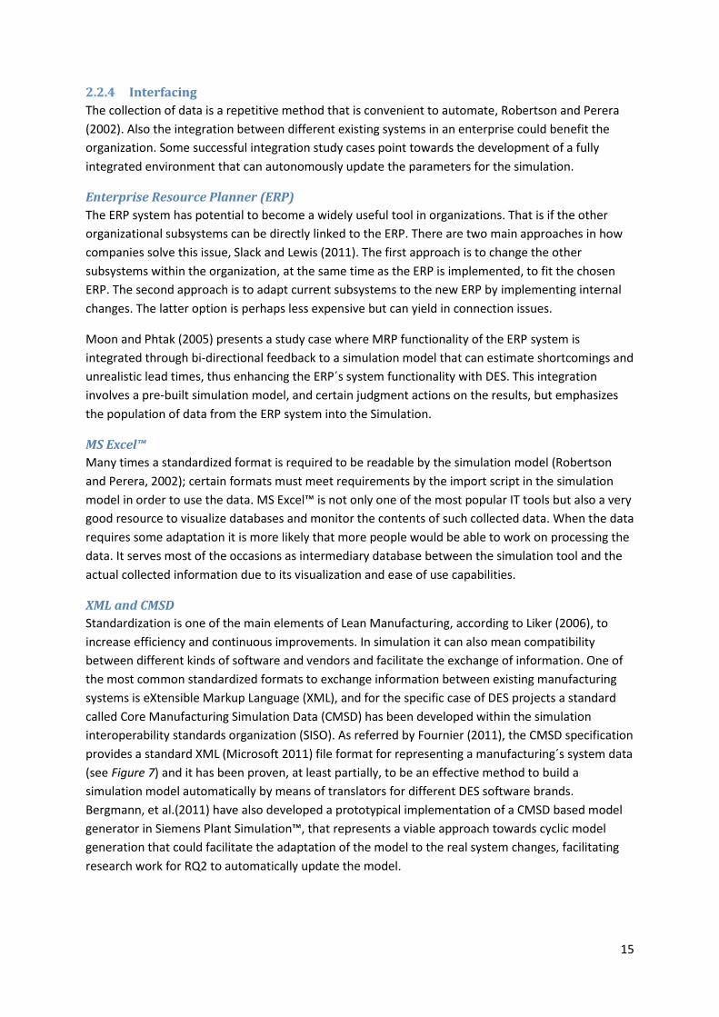
Interfacing 2.2.4
The collection of data is a repetitive method that is convenient to automate, Robertson and Perera
(2002). Also the integration between different existing systems in an enterprise could benefit the
organization. Some successful integration study cases point towards the development of a fully
integrated environment that can autonomously update the parameters for the simulation.
Enterprise Resource Planner (ERP)
The ERP system has potential to become a widely useful tool in organizations. That is if the other
organizational subsystems can be directly linked to the ERP. There are two main approaches in how
companies solve this issue, Slack and Lewis (2011). The first approach is to change the other
subsystems within the organization, at the same time as the ERP is implemented, to fit the chosen
ERP. The second approach is to adapt current subsystems to the new ERP by implementing internal
changes. The latter option is perhaps less expensive but can yield in connection issues.
Moon and Phtak (2005) presents a study case where MRP functionality of the ERP system is
integrated through bi-directional feedback to a simulation model that can estimate shortcomings and
unrealistic lead times, thus enhancing the ERP´s system functionality with DES. This integration
involves a pre-built simulation model, and certain judgment actions on the results, but emphasizes
the population of data from the ERP system into the Simulation.
MS Excel™
Many times a standardized format is required to be readable by the simulation model (Robertson
and Perera, 2002); certain formats must meet requirements by the import script in the simulation
model in order to use the data. MS Excel™ is not only one of the most popular IT tools but also a very
good resource to visualize databases and monitor the contents of such collected data. When the data
requires some adaptation it is more likely that more people would be able to work on processing the
data. It serves most of the occasions as intermediary database between the simulation tool and the
actual collected information due to its visualization and ease of use capabilities.
XML and CMSD
Standardization is one of the main elements of Lean Manufacturing, according to Liker (2006), to
increase efficiency and continuous improvements. In simulation it can also mean compatibility
between different kinds of software and vendors and facilitate the exchange of information. One of
the most common standardized formats to exchange information between existing manufacturing
systems is eXtensible Markup Language (XML), and for the specific case of DES projects a standard
called Core Manufacturing Simulation Data (CMSD) has been developed within the simulation
interoperability standards organization (SISO). As referred by Fournier (2011), the CMSD specification
provides a standard XML (Microsoft 2011) file format for representing a manufacturing´s system data
(see Figure 7) and it has been proven, at least partially, to be an effective method to build a
simulation model automatically by means of translators for different DES software brands.
Bergmann, et al.(2011) have also developed a prototypical implementation of a CMSD based model
generator in Siemens Plant Simulation™, that represents a viable approach towards cyclic model
generation that could facilitate the adaptation of the model to the real system changes, facilitating
research work for RQ2 to automatically update the model.

16
Figure 7 The packages of the CMSD Information Model (SISO 2010)
Data input methodologies 2.2.5
Robertson and Perera (2002) have identified four different types of methods used in companies
today when collecting data for simulation projects, see Figure 8.
Methodology A
Raw data is collected and inserted manually into the simulation model by the model builder. Data
sources are typically shop-floor processes, software and surveys. The approach is simplistic with the
benefit of allowing less experienced model builders to perform the job. The manual parts are often
very time consuming and need to be verified by the model builder, which makes the approach less
desirable.
Methodology B
The main difference when comparing methodology B with A is that the direct manual data input is
replaced with an external spreadsheet. The validation process thus becomes much easier and data
can be manipulated before being inserted in the model. The model can be run without specific
experience or knowledge in simulation model building.
Methodology C
Methodology C takes advantage of existing systems as data storage sources by connecting them with
the simulation to enable automatic updates, instead of using for instance storage in a spreadsheet.
Methodology C is easy to use with the possibility to perform test scenarios and because it is
automated it diminish the time consumption.
Methodology D
Methodology D is taking the input data automatically from the production processes by using for
instance ERP systems within the company. The time and work efforts get reduced drastically but the
process of building the simulation model becomes much more complex. This approach requires
experienced model builders with great specific knowledge. Another drawback is the lack of compiled
data within the company systems. Studies by Skoogh and Johansson (2012) shows that only around 7
percent of companies have the necessary data available at simulation project start.
Further investigations of the data gathering process has been done by Skoogh and Johansson (2009)
through case studies of DES projects in Nordic companies. In their research they found that the

17
actual data collection represented 50 percent of the total time. This was because most companies
still use methodology A with manual data input, due to its easiness of use.
Figure 8 Data input methodologies A, B, C, and D (Robertson and Perera, 2002).
2.3 Supporting Tools in Simulation As mentioned in the previous section, information sources might be required to interface with other
systems that manage information in the organization. Some of these systems serve a special purpose
at planning or production stages and for the purpose of this thesis the most relevant are described in
detail.
2.3.1 Manufacturing Engineering Planning Software - Process Designer™
At production planning stage, assumptions on many input parameters are done because there is no
historical information available. Generally an early rough validation of throughput for the sequence
of operations, resources used, and product, is enough for a simulation model delivery at this point in
time. Nevertheless, if the process information is organized in a structured way in the planning
software and if updated with the latest changes and performance of the running line it can be also
very useful for later stages.
Process designer is an engineering planning application developed by Siemens PLM Software, which
main objective is to generate an electronic Bill of Processes (eBOP). The eBOP defines the sequence
of processes or operations performed in the factory and relate the specific product and resources
that will be used to perform the operation. Furthermore it can organize and relate manufacturing

18
features (spot welds, weld seams and similar) to the product and the operations. It organizes the
information on structured trees and object libraries, which enable several advantages regarding 3D
visualization and re-use.
The three main structures that compose the eBOP in Process Designer are: the operation tree, the
resource tree and the product tree (see (Left) Figure 9,(Center) Figure 10, (Right) Figure 11). The
operation tree shows the sequence of operations, their processing times, and if a part of the product
is consumed at each operation. A specific station operation object is related to a specific station
resource object that contains the resources in which the operation is performed. The product tree is
a structure that shows how the product is composed and represents the Bill of Materials (BOM)
arranged in a manufacturing structure that fits to the structure of the processes; for example, a
certain pre-assembled product part would display as a single object. Finally, resource tree structure
what objects compose each of the plants/lines/stations where the process is performed. It
represents the Bill of Resources (BOR) arranged in a specific structure that resembles the actual plant
layout.
(Left) Figure 9 Operation tree Y352 11-541-000 MPF and Respot
(Center) Figure 10 Resource tree st11_54_020_56
(Right) Figure 11 Product tree Y352 Body
Since several types of products and variants can be processed in the same station, and sometimes,
different processes and resources are required for each different product then several relations
between the Resources tree, Product tree and Operation Tree may exist. Each relation can be done
through “Studies” inside Process Designer. A Study object would delimit the application to display
and work on a specific product variant, specific section of the plant, and a specific operation for that
product. By having this delimitation the software knows which 3D objects and what object
information is required to load in order for the manufacturing engineer to work.
There are several tasks that can be performed with Process Designer, for example:

19
Consuming the eBOM (Engineering Bill of Materials) according to the manufacturing
arrangement to make sure that every part or assembly of the product has been used
(consumed) at a certain process.
Relating the resources available (BOR) at the Plant to be used in the process and use 3D
visualization capabilities.
Visualization of the process flow through PERT charts, Gantt charts, tables, and in the
structure trees.
2.3.2 Layout design software – AutoCAD™
When a simulation model is created, the stations and transport systems need to be located in a
space that replicates the current production layout, and one of the most common industry software
tools for layout design is Autodesk AutoCAD ™. It is a drawing software application specially made
for facilities and construction engineering purposes. The common outputs of this tool are 2D
blueprint files that are easy to explore and manage. For simulation purposes, the AutoCAD ™ layout
drawing is often a good starting point to look into and understand the construction of the studied
system. It also provides good guidance on the exact location of the resources within the physical
space and in many times contain useful visual information about the material or production flow.
2.3.3 Product Data Management – Teamcenter™
In large engineering enterprises there is a need to manage complexity in products that a Product
Data Management (PDM) system can handle (Siemens PLM Software, 2014). A PDM system allows
the engineers to create parts through a structured engineering process workflow. Increased
complexity in a product (variants, changes, revisions and releases) and collaboration between
different departments of an organization are one of the keys for engineering firms to succeed. A
PDM allows having a unique source of information for all the members of an organization where all
the latest changes are immediately visible. It also contains powerful visualization tools and
integration with the most common CAx applications like Catia ™ or NX™. One of the main purposes
of the PDM is to structure the product in an Engineering Bill of Material (EBOM) organized in
functional groups. This structure is commonly exported, sent forward to, and rearranged in the
manufacturing planning application, such as Process Designer ™ transforming the structure of the
EBOM into a new one typically called Manufacturing Bill of Materials (MBOM).
2.3.4 Statistical Analysis software – Minitab™
As shown in 2.1, as part of the simulation project methodology, data collection has shown to be
significantly time-consuming, having a neat process of input data management becomes crucial to
the effectiveness of the project (refer further in section 2.2) . It is required that the data collected
from the available systems is processed into useful information, as mentioned in section Data
Processing. The data processing step in the Input Data Management process could be performed by a
third party application or inside the simulation software. One of the most common industry practices
is to process the sets of data inside MS Excel ™ spreadsheets, or use more advanced statistical tools
such as Minitab ™ to condense the data into statistical distribution functions, which in turn can be
fed into the simulation model.
MS Excel™ provides the user with the regular capabilities found in statistical software while having
the advantage of their extensive user base and knowledge accessibility. If the installed functionalities

20
are not sufficient the user can create Macros that enhance the automation capabilities of processing
data through Visual Basic ™ scripts.
Minitab™ is a specialized statistical software with advanced tools for statistical analyses. Even if the
user base is relatively low, its ease of use is high and visualization of results more intuitive.
2.4 Risk Assessment in Data Input for Simulation The data collection process can involve several potential risks which should be considered before
using in a simulation project. Common risks are touched upon below.
Correctness – Wrong labeling and identification of data or embedded technical problems can
raise issues related to correctness, Skoogh et al. (2012).
Completeness – The data cannot be found in existing sources, Skoogh et al. (2012).
Duplication - Several different sources can provide the same data item. The data source
providing the most accurate data should preferably be chosen here, Robertson and Perera
(2002). Another word used to refer to this issue is consistency, Skoogh et al. (2012).
Accuracy, Reliability and Validity – Data collected must always be verified to be accurate,
reliable and valid before being used as input in a simulation model, Robertson and Perera
(2002). Specifically accuracy has to do with the investigated sources and format of data,
Skoogh et al. (2012). Description of the current state including latest changes has to do with
the validity, Skoogh et al. (2012). As mentioned previously the output of the simulation
model will not be accurate and cannot be trusted.
Timeliness - Typically data is collected from a wide range of sources. This can create an issue
of connected data being available at different times. The data collection process may
become iterative due to this where the modeler needs to connect the data sources when
data is available, Robertson and Perera (2002).
Historical - Considering usage of historical records for data collection may need some
consideration due to risks, Chung (2004). Firstly the production system could be changed
within the time period which the data is collected from. A simulation, using this type of
inaccurate data, will end up with incorrect predictions and cannot be validated. Another
issue which can arise from usage of historical data is the lack of needed data, something
which might not be realized until late in the simulation project.
2.5 Design of Experiments In the experimental phase of the simulation project Design of experiments (DOE) can be used
successfully, Banks (1998). Plant Simulation™ has an inbuilt feature using DOE called the
Experimental Manager. In order to fully take advantage of the tool some background knowledge is
essential. In this section the DOE method will be explained on a deeper level to point a direction of
research and name useful tools to analyze the results of a common simulation case study.
2.5.1 Introduction to DOE
To determine which resources (such as equipment tools, conveyors etc.) and settings which have the
most influence on the process performance a set of experiments is made, thus enabling changes

21
towards a more optimal performance. DOE is an efficient methodology of performing several
experiments at the same time, Montgomery (2000). The aim of a DOE is to use a minimum of
resources for a maximum of information, which implies several factors with a smaller number of
samples, Cavazzuti (2013), Bergman and Klefsjö (2010). This reduces the cost compared to using the
one-factor-at-a-time experiment, Bergman and Klefsjö (2010). The following DOEs are presented in
below sections:
Full factorial design
Fractional factorial design
Explanation below relates to terms that are of interest and importance when investigating DOE,
Cavazzuti (2013).
Noise is the term used for errors in DOE. Statistical methods are used to diminish the effects
on the results caused by noise. General groupings of these statistical methods are
randomization, replication and blocking, Cavazzuti (2013), Bergman and Klefsjö (2010).
Randomization concerns the order that the experimental runs are made. The order is
randomized to remove potential influence from the previous to the following or potential
ability to predict experimental results.
Replication is used to duplicate a specific setting in order to be able to run that setting
several times. This is done to verify quality and correctness.
Blocking is used for isolation of events which are disrupting the experimental main result.
These events can thus be blocked out and their effects can thereby be prevented.
2.5.2 Full factorial design
Creating a test plan before the experiments is started also yields in lower costs, Bergman and Klefsjö
(2010). A full factorial design utilizes this strategy with a plan that includes which factors to be
studied, such as:
Buffer size
Station throughput time
Product mix
Table 4 Design matrix from Bergman and Klefsjö (2010)
Run no. Main factors and interaction
A B C AxB AxC BxC AxBxC y 1 - - - + + + - 67 2 + - - - - + + 79 3 - + - - + - + 59 4 + + - + - - - 90 5 - - + + - - + 61 6 + - + - + - - 75 7 - + + - - + - 52 8 + + + + + + + 87
Estimated effects
23 1.5 -5.0 10 1.5 0.0 0.5

22
Then the two levels are decided on and set for each factor, one high and one low value. The high
value corresponds to a “+” and the low to a “-“. The experiment then runs for each test condition in a
randomized order with, as in this case of three factors, eight runs. Estimation on the effects of the
experiment can be assessed using the average of the difference in high and low values. By
performing experiments like this the interaction of factors can be identified, an effect which is not
possible to estimate when performing a one-test-at-a-time experiment. Estimated effects are then
presented in a design matrix (see Table 4) where a clear visualization provides an immediate
overview of factor impact and in between interaction.
2.5.3 Fractional factorial design
In the case when three factors are investigated, and two of the factors A and B do not interact, a
fractional factorial design can be performed. This yield in even lower resource utilization as fewer
runs needs to be performed to see the interaction on factors A and B by the factor C. In a scenario
with three factors only four runs are needed. If the A and B factors would have had interaction they
would have said to aliased and a full factorial design would have been necessary. Fractional factorial
design can be extended to more factors where there are reason to think only two factors actually
interact, Bergman and Klefsjö (2010).
2.5.4 Statistical process control
Statistical process control (SPC) is implemented to find assignable causes of variation in order to
eliminate them to stabilize and perform supervision of processes, by taking a sample of observation
at certain time intervals. Found causes are either assignable, and can be directly linked as a major
contributor to variation, or common, which are more general cause contributors to variation. When a
process is in statistical control the standard deviation and mean are known. The process is then
stable and the quality indicator are within calculated limits e.g. control limits. For further depth in the
SPC subject see Bergman and Klefsjö (2010).
An example of DOE experimental design with two processes follows based on an introduction
chapter by Goos and Jones (2011).
Sample size:
Mean:
Average:
Standard deviation: √
Variance:
23
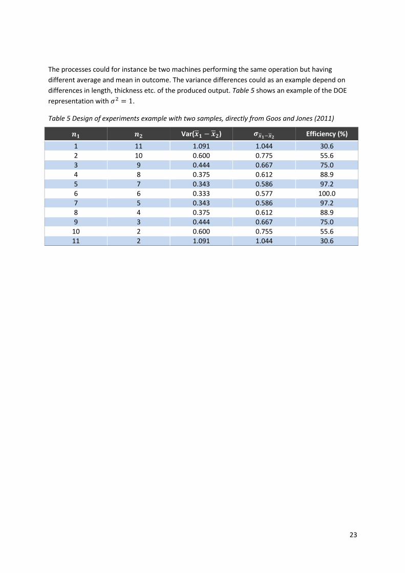
The processes could for instance be two machines performing the same operation but having
different average and mean in outcome. The variance differences could as an example depend on
differences in length, thickness etc. of the produced output. Table 5 shows an example of the DOE
representation with .
Table 5 Design of experiments example with two samples, directly from Goos and Jones (2011)
Var( ) Efficiency (%)
1 11 1.091 1.044 30.6
2 10 0.600 0.775 55.6
3 9 0.444 0.667 75.0
4 8 0.375 0.612 88.9
5 7 0.343 0.586 97.2
6 6 0.333 0.577 100.0
7 5 0.343 0.586 97.2
8 4 0.375 0.612 88.9
9 3 0.444 0.667 75.0
10 2 0.600 0.755 55.6
11 2 1.091 1.044 30.6

24

25
3 Methodology Focus on the thesis lies within the data collection process in order to perform a gap analysis in VCT.
According to the thesis purpose, the main objective of the gap analysis is to create a foundation,
which supports a future automation of simulation models through the StreaMod project. To
understand what the simulation requirements are, a simulation model is set up on the area of the
project scope. The methodology for the general simulation model creation is based on the theory
described in section 2.1 and 2.2, and goes into depth for the input data management.
According to Banks simulation project
methodology a simulation project was started.
Focus was mainly on the iterative process between
the conceptual model and the data gathering.
Special attention was given to the data collection
process and general input data management, see
Figure 12, which is described further in the
following section, 3.1 Input Data Management
Methodology.
3.1 Input Data Management
Methodology As describe in the Theory chapter the thesis is
outlined accordingly:
1. Identify and define relevant parameters
2. Specify accuracy requirements
3. Identify available data
4. Choose methods for gathering of not
available data
Milestone: Will all specified data be found?
5. Create data sheet
6. Compile available data
7. Gather not available data
8. Prepare statistical or empirical
representation
Milestone: Sufficient representation?
9. Validate data representations
Milestone: Validated?
10. Finish final documentation
Compile available data Gather not available data
Create data sheet
Identify and define relevant parameters
Specify accuracy requirements
Identify available data
Choose methods for gathering of not available data
Will all specified
data be found
Validate data representations
Sufficient
representation?
Validated?
Finish final
documentation
Prepare statistical or empirical representation
Yes
Yes
Yes
No
No
No
Figure 12 Input data management methodology, Skoogh and Johansson (2008)
26
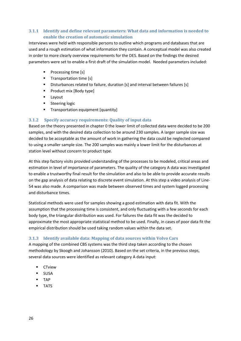
3.1.1 Identify and define relevant parameters: What data and information is needed to
enable the creation of automatic simulation
Interviews were held with responsible persons to outline which programs and databases that are
used and a rough estimation of what information they contain. A conceptual model was also created
in order to more clearly overview requirements for the DES. Based on the findings the desired
parameters were set to enable a first draft of the simulation model. Needed parameters included:
Processing time [s]
Transportation time [s]
Disturbances related to failure, duration [s] and interval between failures [s]
Product mix [Body type]
Layout
Steering logic
Transportation equipment [quantity]
3.1.2 Specify accuracy requirements: Quality of input data
Based on the theory presented in chapter 0 the lower limit of collected data were decided to be 200
samples, and with the desired data collection to be around 230 samples. A larger sample size was
decided to be acceptable as the amount of work in gathering the data could be neglected compared
to using a smaller sample size. The 200 samples was mainly a lower limit for the disturbances at
station level without concern to product type.
At this step factory visits provided understanding of the processes to be modeled, critical areas and
estimation in level of importance of parameters. The quality of the category A data was investigated
to enable a trustworthy final result for the simulation and also to be able to provide accurate results
on the gap analysis of data relating to discrete event simulation. At this step a video analysis of Line-
54 was also made. A comparison was made between observed times and system logged processing
and disturbance times.
Statistical methods were used for samples showing a good estimation with data fit. With the
assumption that the processing time is consistent, and only fluctuating with a few seconds for each
body type, the triangular distribution was used. For failures the data fit was the decided to
approximate the most appropriate statistical method to be used. Finally, in cases of poor data fit the
empirical distribution should be used taking random values within the data set.
3.1.3 Identify available data: Mapping of data sources within Volvo Cars
A mapping of the combined CBS systems was the third step taken according to the chosen
methodology by Skoogh and Johansson (2010). Based on the set criteria, in the previous steps,
several data sources were identified as relevant category A data input:
CTview
SUSA
TAP
TATS

27
Where CTview and SUSA are data sources applications, TAP is the MES deciding product sequence,
and TATS is an internal unofficial SCADA production website. CTview provided history data for
transport and processing times combined with product mix. Disturbances with classification were
found in SUSA. TAP provided production sequence and buffer numbers. TATS distributed information
about buffer sizes, mainly in form of pictures. An overview is shown below in Figure 13. For more
detailed information about the databases see Appendix A-C.
3.1.4 Choose methods for gathering not available data
Category B and C data was addressed at this step starting with a visual overview of unavailable and
uncollectable data together with the available, see section 2.2 .
From the classification of category B data a plan was created based on manual attempts on how to
extract and calculate the wanted information. Several program functions were investigated including
AutoCAD™-drawings, MS Excel, Minitab, Mitsubishi’s PLC, Process Designer, and Plant Simulation.
This step included steering logic, layout, data quality, and general in-between lines transportation
findings.
Milestone: Will all specified data be found?
As a validation of the previous steps the question was asked and confirmed, although not all
necessary data could be found directly, in order for the process to move on to step 5.
3.1.5 Create data sheet
Based on the characteristics of Plant simulation and available data format, data sheets were
structured with consideration to previously defined parameters. All data was placed in the same
folder with subfolders depending on content. Naming of data documents was standardized.
3.1.6 Compile available data
Data from SUSA was collected from week 1 to week 14 of year 2014. Due to shorter storage times for
data in CTview, it could only be gathered from week 9 to week 14 of year 2014. Based on station and
TATS
CTview
SUSA
TAP
Cycle time
Processing time
Product mix
Disturbance
Product mix
Sequence
History of processed bodies
Buffer sizes
TATS
Figure 13 Overview of VCT databases

28
depending on data base source, Ctview or SUSA, the data was gathered in two specific folders. The
reason to this was the idea of keeping the data transparent and clear to users outside of the thesis.
Two tailored macros for each database were created in order to speed up the data gathering process
and making it more automated. By using the macros a conversion to a more usable time format was
made. From these macros appropriate calculations and conversions, based on the defined
parameters from the first step, was made such as clean cycle times, interval, duration etc.
For information which could not be found and downloaded to be used in MS Excel, there was only a
process of collecting the data manually. However, as can be seen in the results in chapter 6 the
performed gap analysis points out which information this was and where it can be found.
3.1.7 Gather not available data
Category B data was gathered and calculated by using production design programs such as Process
Designer (PD) and AutoCAD™. The majority of the data found here was concerning transportation.
Factory visits was another source which provided updated real time information mainly about buffer
sizes, layout, and production steering logic. Accordingly the data found using these methods is
presented as gap analysis results in chapter 6.
3.1.8 Prepare statistical or empirical representation
The data sheets created in Excel with data was organized to allow statistical evaluations with data fit
within Plant Simulation. Based on the presented theory on statistical methods and general usage of
data in DES, the different types of data were evaluated accordingly.
Milestone: Sufficient representation?
Goodness-of-fit test were performed on the disturbance data. In cases where there was no data fit
the empirical distribution was chosen as planned in the early steps. All data was questioned if having
sufficient representation.
3.1.9 Validate data representations
A data validation process was made together with a simulation expert and by internal meetings
where the data compilation process was explained thoroughly together with output and input format
explanations. It was found that not all data could be validated to be sufficiently represented or with
high enough quality.
Milestone: Validated?
A systematic approach was utilized to confirm that all data representations had been questioned and
verified as accurate or labeled otherwise. At this step it was clear that not all data could be validated
to hold high enough quality for use in a simulation model.
3.1.10 Finish final documentation
Final documentation with examples of data sheets was finished and the gap analysis findings were
added to the results in chapter 6, together with general results for the conceptual simulation model.

29
4 Simulation Model The simulation model case of the Body Shop Factory was developed in order for the authors to
understand what kind of information was needed and where it was extracted from, in the current
production system. Findings regarding the different simulation input parameters used in the DES
model creation, see Figure 14, are presented in this section. The results of the simulation model itself
could be verified but not completely validated (Sargent, 2010), since it has been detected to hold a
significant lack of quality regarding the data logged in the production database. Correcting the alarm
and process times log is out of scope of the thesis but further discussed in Chapter 8 Discussion &
Suggestions.
Figure 14 Simulation layout with Sankey Diagram for each line products

30
4.1 Empirical Data After initial factory visits and introductions to the available production systems, the reliability of the
logged production information seemed to be compromised by the most recent major changes. The
thesis team decided to record production in stations of Line-54 at specific times, which involved the
Framing station, and compare the logged data against what was observed in the videos. Several
inconsistencies were found regarding alarms and processing times logged in information. The most
relevant observation is that failure alarms cause problems with the processing times registers, for
example it has been observed that when a robot has a technical failure in the middle of the process
the registered processing time will include the duration of the failure.
4.2 Steering Logic The steering logic defines how the material flows through the lines and what kind of conditions that
must be true in order to pass the parts on to the next station and/or carry out certain additional
actions. This was particularly relevant when modeling the logic at the BSI lines (11-56 and 11-57). In
these lines, a product type specific fixture must match the production sequence and in case of a
mismatch the Electric Overhead Monorail (EOM) elevator system must activate to change the current
fixture for the correct one. In the simulation model the exit control at stations 11-(56/57)-Hiss (refer
to Appendix D), and the predecessor station define the behavior of this logic along with the EOM exit
strategy on the top floor. It has been detected that the logic differs on Left and Right sides mainly
because the layout configuration and number of stations are different on each side.
This behavior of the production lines logic is described in the document “Driftanvisning” as
mentioned in section 0. The pitfall, regarding documentation method for this specific case, is that
even if the supplier updated the information, it is generally not always the case. Informal interviews
with manufacturing engineers revealed uncertainty in the update validity of these documents. The
most efficient resource that the authors used to understand the steering logic were factory visits and
informal interviews with the people involved in the production lines. This last fact revealed
unavailability of steering logic information in a system, which would be needed in order to automate
a DES model creation.
4.3 Processing times As explained in section 5 below, the Virtual Device contains the logged data about the processing
times of the stations, whereas through CTview and/or TATS the team was able to collect logged data
from week 9 to week 16 of 2014. In order to work with the logged processing times and get a more
accurate representation of cycle times three possibilities were explored.
The first approach was to identify the failed cycle times by filtering all cycle times that last more than
90 seconds for each product type. This is already a common internal practice to obtain a quick
representation of the cycle times that has shown fairly good results without consuming much time.
A second approach is a proposition that the authors came up with in order to obtain more accurate
representations of cycle times. This approach filters the start-to-start cycle times that do not contain
any kind of disturbance. This proposition is made assuming that three main conditions are always
true. First, that the start-to-start cycle timestamps are triggered when a new product enters one
station until the next product enters into the same one station. Second, that all kinds of

31
disturbances; e.g. failures, starvations or blockages, registered in SUSA have a precise start
timestamp. Third, that both of the logging systems are running under the same clock time.
With the use of a VBA script in MS Excel™ failures start timestamps could be located between the
start-to-start timestamps and therefore those cycles that contain any failure could be identified and
deleted. Additionally, the cycles out of regular working shifts were also deleted. The expected result
is only cycles that contain pure processing time and transport times. Nevertheless, after applying this
last method to the collected dataset, the resulting cycle times contained cycles that were longer than
a clean cycle time expectation. This unexpected result means that some of other disturbances are
not logged in the system or that the start timestamps are inaccurate.
The third approach is a combination of the first two approaches, which the thesis team believes
would lead to the most accurate results possible.
4.4 Disturbances The disturbances logged into SUSA are the largest issue regarding logged data, section 5.1.3. It has
been found that the alarm monitoring resolution is very low, taking around 25 seconds for the VD to
detect updates of a triggered alarm in the PLC´s. This can be one of the main causes of logging errors
in disturbance durations since the alarms may overlap; e.g. when the operators enters inside a
protected area to fix the failures might also trigger the door alarm.
Also as mentioned in section 4.1 on empirical data, there is an unclear definition of how the alarms
affect processing times in the Virtual Device. The team considers logged disturbances as inaccurate
information but assumed that the change of state (from normal to alarmed) timestamp is accurate
for the simulation model creation.
4.5 Transport The transport times between stations was included in the start-to-start cycle times, nevertheless
several conveyor systems were modeled on top of the AutoCAD drawing. The conveyors that also
acted as buffer places were undocumented and it was not possible to extract information out of the
other software applications. The steering logic of the transport systems, for example the EOM at the
BSO lines had a very complex behavior when the sequence of products was not stable and several
fixture changes were required to cope with the correct sequence. Other discovery was that the left
and the right side lines are different. The right hand side has more stations in the BSO line and more
fixtures can be in the system, while the LH had fewer amount of fixtures.

32

33
5 Information map at VCT To start answer RQ1 a mapping of the information sources at VCT is presented in this chapter
grouped as: Input data source, Program software sources, and support information, see Figure 15.
The chapter aims mainly at presenting the systems at VCT to make the reader more familiar with
them.
RQ1 What are the requirements for input data to generate a simulation model that addresses a
common engineering question?
Figure 15 Information mapping of data and information sources at VCT
5.1 Input Data Sources This section presents the findings regarding the actual production floor data sources, providing
empirical real time data, which were explored and used when building the simulation model for the
study case at VCT. All the data from the production lines PLC's is collected automatically through a
system called Virtual Device (VD), then several applications can present the data in different ways to
the user. Each section describes the purpose and data content of the applications that run over the
VD.
TAP Systemdokumentation – Sido och Takbeordring i
FAB 11
Virtual Device (VD)
Production floor (PLC)
TAP
KOP
SUSA TATS CTview Driftsanvisning
Mitsubishi PLC
eMS Server PLM Server
Process Designer
Plant Simulation
Team Center
Overview of Sources for Input
Data and Information
Input Data Sources
Program Software Sources
Support Information
AutoCAD™ Layout

34
TAP 5.1.1
TAP (Torslanda A-shop Planning software) is an application that manages all the product orders
through the plant. Sequencing and ordering of body types are done through TAP. The user can track
the location of a specific car body; find detailed information on timestamps at every station of the
plant; specific car model; and historical production information. KOP system, which runs over TAP, is
used by production planners to control orders in production.
CTview 5.1.2
CTview, also known as OEE Portal, is an application that runs over the Virtual Device that presents
the collected data from the production floor in a database format that can be copied or exported
into spreadsheets for further analysis, see Figure 16. The user can find different columns with
information specific of a certain location of the factory, which contains all the timestamps of the
products that have arrived to the station, the processing time, cycle time, transport time and
processing time for each robot in the station. See Appendix A for instructions on how to use CTview.
CTview is a tool within the OEE portal that allows the user to get different registered times for a
specific station in the plant. This information can be filtered, sorted or exported on-demand.
Figure 16 Body shop production in VCT
SUSA 5.1.3
SUSA is an application that registers all the disturbances in the factory. It classifies disturbances into
different kinds and registers information about the body type, duration of disturbance and start/stop
time of each failure. It can further filter the failures depending on type or data. See Appendix B for
further instructions on how to use SUSA.

35
TATS 5.1.4
TATS is an unofficial SCADA website where production data is visualized. As CTview, TATS can display
similar production data as well as buffer sizes and number of fixtures for the outer sides. It can also
export around 45 days of production data directly to a MS Excel™ file, see Appendix C for further
information.
5.2 Program Software Sources at VCT Process Designer™ is the software where VCT plan all the production processes at VCT, which could
benefit the StreaMod project objectives. Secondly Teamcenter™, which is also a Siemens™
software, concentrates product information in a single source and has the potential to include
manufacturing information in the future, addressing RQ2 in a longer term. This section present what
kind of information, useful for the simulation modeler, can be found in each source at VCT.
Process Designer 5.2.1
As mentioned previously on section 2.3.1, Process Designer™ stores production planning
information at VCT. The information that it contains is developed in collaboration with line builders.
The requirements and specification of deliveries are standardized in a recently created document
"VCC Manufacturing Simulation Specification".
Some usage characteristics of Process Designer at VCT are:
One single Bill of Resources can be found in Process Designer containing the 3D CAD and
resource tree structure available in the TA Plant. The tree structure and naming is standardized.
Figure 17 and Figure 18 show an example of a standard resource tree.
Additionally there is a specific BOP for each product type. Depending on the product variant, the
process at each station may vary; therefore different BOPs are related to the Plant BOR.
Figure 17 (Left) Resource tree in Process Designer
Figure 18 (Right) Resource tree at a deeper node level in Process Designer
After the BOP has been defined in Process Designer, the Station level robotics operations can be
defined at Robot level. Process Simulate is used to generate all the paths and actions of process for
all the robots in a station in order to create and validate virtually the process of the different car
bodies. The objective of Process Simulate is to output the robot program that will be downloaded
later to the robot.
Addressing RQ2, it has been explored by the thesis group the possibility to use the automatic export
to a detailed simulation model that is apparently available in Process Designer™, nevertheless the

36
versions of Plant Simulation™ that are supported are too old to be used and Siemens PLM
Software™ has taken the decision to not further support this feature anymore, see Figure 19.
Figure 19 Simulation export only support until version 9.0 of Plant Simulation
For StreaMod project purpose, which deals with the possibility of automating the creation and
update of simulation models, there are some characteristics from Process Designer that could tell the
programmer of a script or the script designer what information could be extracted from it, especially
the one regarding process, consumed parts and material flow without considering the transport
systems. Some of these characteristics will be mentioned later on Chapter 6.
Teamcenter™ 5.2.2
VCT uses Teamcenter™ to generate the BOM for each of the products including all variants and
revisions that they might have. It contains a module called Manufacturing Process Planner, in which
the user can setup a similar BOP as Process Designer does. Nevertheless, this has not been
implemented in TA. The thesis team did not found relevant information in this source for a DES
model and is not included in Chapter 6 Gap Analysis. If in future the manufacturing module is
implemented, then it would be interesting for RQ2.
5.3 Information Sources Other sources of information that do not belong to any CBS or actual production data were explored
and are presented in this section. These sources are found to be of possible relevance as support
documentation and might be useful in the creation of a DES model.
Driftsanvisning 5.3.1
Driftsanvisning ("operating instructions" in English) is a manual that is delivered by the line builder,
which provides written information about the order of value adding process steps for each station in
a specific line. This kind of documents can be found in the organization VDOC system. It contains also
a list of equipment for each of the stations in the line. The process descriptions are furthermore
specified for each body type. The document is written in Swedish and is most similar to a description
of the station operation.
37
Mitsubishi PLC 5.3.2
The steering logic of the production system, including transportation systems and alarms, in the TA
factory is controlled by Mitsubishi™ PLCs. The thesis team explored the possibility to find useful
information in the PLC programs or comments to model the steering logic. Inconveniently, the PLC
programs required a high level of expertise in programming to understand the logic and the
comments did not bring any value to the DES model creation. This possibility was disregarded and
not further explored.
AutoCAD™ Layout 5.3.3
Other supporting tools for automotive industry are the layouts that the line builders design in order
to build the equipment in place. One of the most common formats is to have an AutoCAD ™ drawing
that contains the relevant equipment and surrounding objects that will be installed in the facilities.
Many times equipment that is not directly part of the main processes are omitted in other systems,
for example with transport of storage resources that do not add any value to the product but whose
characteristics affect the production performance, the engineer can therefore extract dimensions
and estimate capacities out of the drawings. At VCT AutoCAD™ is used for the production processes
and displays stations. It is used as background pictures for DES projects within VCT and as an initial
understanding of the process flow.
TAP Beordring 5.3.4
The ordering of products, such as sides, roof and body type, are described in the manual TAP
beordring (“ordering” in English) which can be used as a complement to the TAP system. Here it is
described from which station a signal is sent to initialize manufacturing start and how the products
are queued. The production can therefore be said to be pull-based as products are only produced if
there is a corresponding body type in upstream processes and thus a customer demand.

38

39
6 Gap Analysis
RQ2 How can a simulation model be integrated to the production data sources to automate the
model creation and update of the required input information?
RQ2 is answered in the following section through the study case at VCT where a gap analysis over the
input data in VCT is presented. Figure 15 provides an overview of relevant sources for data and
information needed in order to create a DES model. The gap analysis is presented according to the
theory-introduced category A, B and C data, divided in station- and resource level, and
transportation. These in turn, were presented under the subheads introduced in Figure 15 input data
sources; support information and program software.
6.1 Category A Data: Available Data and information presented in this section is classified as available and collectable. The quality
are however questionable for some of the parameters. Table 6 provides a summary of the A data
based on parameter and related information are divided into four columns with source, a short
explanatory description, when the data is logged, and preferred update interval for the StreaMod
project. The update interval is defined in order to obtain an approximate number of 250 samples of
the same kind of data, depending on the occurrence of a registry a different interval is needed.
Table 6 Gap analysis category A data
Gap Analysis
Category A data: available
Station- and Resource Level
Parameter Source Description Logged Update
Cycle Time CTview
From start-to-start.
35 days detailed info
Real time automatic. 2 weeks
TATS script
From robot start to last
robot end
45 days basic info
Real time automatic. 2 weeks
Processing Time CTview
From robot start to last
robot end
Not accurate!
Real time automatic. 2 weeks
Disturbance SUSA
Start of failure related: P,
K, T or U
1 year of historical data
Monitor change every
25 seconds due to old
PLC.
Monthly
- Personnel (P) SUSA
When maintenance
personnel open the station
door. Comments in SUSA
for more precise problem
definition.
Every 25 seconds due
to old PLC. Monthly

40
- Quality (K) SUSA When PLC detects a
quality error
Every 25 seconds due
to old PLC. Monthly
- Technical (T) SUSA Robotic failure,
maintenance failure etc.
Every 25 seconds due
to old PLC. Monthly
- Maintenance (U) SUSA Scheduled maintenance of
e.g. robots
Every 25 seconds due
to old PLC. Monthly
Product Mix CTview / TATS Related to cycle time and
processing time Real time automatic. 2 weeks
SUSA Related to disturbances Every 25 seconds due
to old PLC. 2 weeks
TAP Deciding on sequence
order Real time automatic 2weeks
Transport CTview
From end of processing to
start of processing.
Definition unclear.
Observations showed a
different time than the
time stamp.
Real time automatic. 2 weeks
Layout TATS
Overview with line name
and station number. Only
bottom floor available.
Static. Every 3-6
months
Auto CAD Detailed view with line
name and station number. Last update ?
Every 3-6
months
Process Flow TATS Real time color coded
connected to body type Real time automatic.
With process
changes
Driftsanvisning
Description over the
station logic and
resources.
By body type release.
Last update 2012.
With process
changes
TAP -
systembeordring
Document describing inner
and outer side ordering
and roof.
(Line-51/52/56/57 and
/54)
Static.
Last update 2007.
Static
Process Designer PERT and Operation tree By body type release Every 3-6
months
Resources PD
All objects in a station and
material input
(consumption)
Weekly/Monthly. Weekly/Mont
hly
Transport Parameter Source Description Logged Update
Product Mix TAP Sides to 11-54-020. Real time automatic. Every 2nd
week
TATS Percentage mix under the
head line TA1 Palett Mix Static.
Every
month

41
Layout Auto CAD Upper floor OEMs. Static.
With
process
changes
Process Flow Auto CAD Arrows in upper floor
drawings. Static.
With
process
changes
Resources TATS Number of outer-side
fixtures. Needs update. Static.
Every 2nd
month
The update interval should be viewed as a way to assure the quality of the data collected since it
might have inaccuracies normally due to changes in production lines or products.
Input Data Sources 6.1.1
In the TA factory (body shop) at VCT there are several input data sources that contain relevant data
and/or information for the creation of a DES model.
CTview
TAP
SUSA
TATS Script
This data is generated and stored through a SCADA system called “Virtual Device” (VD) which
registers the different PLC signals timestamps sent from the shop floor processes. TATS Script and
SUSA are the two main data sources used in the thesis to extract information
Both CTview and TATS Script provide the data for processing and transportation time connected to
each station. A limitation with CTview, as a data source, is the short storage time because the query
for historical data can be a maximum of 35 days. Thus there is a limitation in the storage time.
However, by using TATS an MS Excel download can be reached which can provide additional data
over a total of 45 days. The TATS option requires a manual change of station number directly in the
webpage name in order to find and output data for the desired station. Another limitation with the
Start of Cycle: YYYYWWDHH:MM:SS
Processing Time: SS,S
Transport Time: SS.S
Cycle Time: SS.S
Figure 20 CTview

42
TATS option is the missing robot specific processing time, which can be found in CTview between
Transport- and Cycle Time, see Figure 20.
SUSA is, as explained in section 5.1.3, the data source for disturbances connected to each station. At
resource level it is possible to find failure cause to some extent related to the classification explained
below. By typing in the station name, e.g. 11-54-020 (the framing station), the following information
of interest for DES application can be obtained.
Disturbance classification: FS (Blocking), VS (Starvation), T (Technical failure), P (Personnel
related failure), U (Maintenance), and K (Quality related failures)
Disturbance Start
Disturbance Stop (Not accurate)
Loss
Product Mix (V60,V70,S60,S80)
Technical failures can be traced to the object causing the alarm but is not exactly defined. Figure 21
shows an example of how SUSA looks and in what format the information can be found.
The start of disturbance timestamp has proven to be close to accurate, but the stop timestamp is
not. This fact is presented further in section 6.2 under category B data.
TAP is the ordering system in VCT and sets the body type sequence. As can be seen in Figure 22 the
system has a Swedish operating language. Since TAP logs the Escort Memory (EM)-card at every
station it also provides more information usable for simulation purpose. Ordering point of complete
sides, inner sides, roof and body type can be found. There is also the possibility to see real time
buffer sizes between Lines.
The lower picture in Figure 23 shows an example from the BEO option with ordering of complete-
left-side (SIDVK), complete-right-side (SIDHK), and roof (TAK) combined with palette ID-number, e.g.
“51-9-79/3”. For the sides, the first two numbers, 51, indicates which Line-buffer the palette is
Disturbance Start: YYYYWWDHH:MM:SS
Loss: H:MM:SS
Disturbance Stop: YYYYWWDHH:MM:SS
Disturbance: FS/VS/T/P/U/K
Product Mix:: V60-70/S60-80
Figure 21 SUSA

43
ordered from. This is not true for the roof. The body type characteristic (Egenskaper) can be read in
the column farthest to the right (see Karosstyper A – B Fabrik for body type identification table).
Note how the naming here is slightly different from SUSA and CTview. In SUSA the station naming is
standardized to “11-54-020” and in CTview stations use the prefix "A", e.g. "A11-54-020". In TAP it is
“1154020” without the “-“. It can be thought of as a small thing but when retrieving the data from
the systems this creates issues because the retrieving process cannot be replicated.
Figure 22 TAP introduction page overview
Figure 23 BEO option overview in TAP
Program Software Sources 6.1.2
Some information available for the simulation user that is stored in Process Designer, is the eBOP
that can be displayed in the form of a PERT diagram (Program Evaluation and Review Technique), see
Figure 24. In the PERT diagram the sequence of the operations is displayed along with the material

44
flow. The diagram also displays the part sources and where parts are consumed. It also can display
the resources used on each station when they are related to the process and the allocated time for
the operations.
Figure 24 PERT diagram from Process Designer
Other available structure loaded in Process Designer by line builders, according to Volvo specification
document is the resource tree (see Figure 25). The simulation modeler can view the components that
compose the stations, lines and areas of the factory. If the availability parameters of the components
are known then they can be used to set up the proper availability in the resources of the simulation.

45
Figure 25 Resource tree and hierarchy
Support Information 6.1.3
All data and information cannot be directly found in the input data sources or program software
sources. Due to this shortage additional support information has been investigated as potential
alternative source options. The following document and program introduction are the result of this
investigation and is found to contain relevant information for the purpose of future automatic
generation of DES models.
Driftsanvisning (operation instructions)
Mitsubishi PLC
Auto CAD Layout
TAP Systemdokumentation (TAP system documentation)
The Driftsanvisning manuals contain information about the logic for each station in an entire line
related to each body type. However, the body types are expressed in terms of Y286 instead of S80
etc. just as in TAP (see Karosstyper A – B Fabrik for the detailed body type labeling and description,
not included in thesis). It is useful for the understanding of the process in connection to walking the
line and building a simulation model. The document is also updated since the introduction of the
latest car model, the S60.
All steering of lines are done through the Mitsubishi PLC. Initially it was intended to look through the
PLC to gain understanding of how the steering is programmed. Because the PLC is of an outdated
version this became very difficult. It is programmed for each station according to the Mitsubishi
program structure. There are few comments which are written with a lack of standardization, and
thereby attempts to follow the code are difficult - unless the user has previous experience in the
software.

46
Auto CAD was found useful to get a visual overview of both top and bottom floor. Figure 26 is an
example of a drawing with overview of the thesis delimited area, line-51/52/54/56/57.
Robots are surrounded by circles and are easy to see when zooming into the drawing. On the side of
each station the station name can be read e.g. “– 100”. This can be seen in the right circle in the
drawing, which shows an enlarged section. The individual robot number can also be read and
information as displayed here “pallställ” (“pallet rack” in English). The squares indicate body position.
TAP beordring describes the logic behind steering and ordering of roof, BSI and BSO. It is very clear
and gives precise description. By reading this document the understanding of how TAP works
becomes clearer as it is a type of description manual to TAP.
Figure 26 Auto CAD drawing over delimited production body shop area in VCT

47
6.2 Category B Data: Available But Not Collectable Data and information in this section are available but has not been gathered due to limited
accessibility or the need of complicated procedures involved in the gathering process. All fields filled
in with orange in Table 7 of this section are connected to category B data.
Table 7 Gap analysis category B data
Gap Analysis
Category B data: Available But Not Collectable
Station- and Resource Level
Parameter Source Description Logged Update
Availability Supplying Line-builder Info can be reached if requested.
Not standardized available in VCT.
No.
Disturbance SUSA Failure related: P, K, T or U
Logged but with low quality.
Every 25 seconds due to
old PLC.
Cycle time disturbance CTview or SUSA Can be combined by using
timestamps.
No.
Processing time
disturbance
CTview or SUSA Can be combined by using
timestamps.
No.
Transport disturbance CTview or SUSA Can be combined by using
timestamps.
No.
Disturbance cause SUSA Not sufficient documentation on
causes. Operators do not add info
standardized.
At failure.
Transport Parameter Source Description Logged Update
Product Mix TAP Real time automatic.
TATS Shows static figures which are not
updated regularly of fixtures for
outer and inner sides. (Line-
51/52/56/57)
Static.
Layout Auto CAD Different versions available. Static.
Needs update.
Input Data Sources 6.2.1
The disturbance data is logged and stored in SUSA at a continuous basis. However, the disturbance
data has insufficient quality. The actual disturbance duration time cannot be identified as the alarms
continue to send throughout the processing time. That is from start of disturbance until the entry of
a new product. Thus even if the failure has been corrected the disturbance alarm will continue. This
was realized during time studies of videos where the alarm times in SUSA for a specific body was
matched with the video times.

48
In the current input data sources used at station level there is no interconnection between CTview
and SUSA. Processing time and cycle time are not displayed connected to disturbances. Since the
cycle time is affected by disturbances it is necessary to connect the two parameters, in order to reach
a good input data quality for the simulation model. This can be done with the help of the time
stamps. With the creation of a macro in MS Excel™ the connection has been accomplished through a
cleaning process. All cycle times affected with disturbances have been removed in order to find the
correct processing time.
At resource level the situation is the same with no interconnection between CTview and SUSA. The
data quality is questioned and considered insufficient at station level and is not trustworthy at
resource level. Hence if data at resource level is desired a process on gathering the data needs to be
assigned. At the moment the data should be available at in-house virtual simulators of PD. As
mentioned in the previous section there is a cause classification connected to SUSA. It is possible to
find T-failures and alarms triggered by a specific robot. Maintenance personnel also fill in the
comments when opening the door to a station, which triggers a P alarm. The yellow marking is due to
lack of data here and the quality. Standardization in the comment writing is limited and the operator
shows a lack of motivation to write comments due to insufficient background knowledge and
understanding.
Program Software Sources 6.2.2
Even if the processes can be displayed in PERT diagrams as mentioned in section 6.1.2, no process
times or other simulation attributes are fed. Also it can be seen that no transport systems are
considered as part of the process. It can be seen from Figure 27 that certain attributes, with
importance for DES, could be added to the process objects and thereby be passed forward to the
Simulation software. Even if these attributes are designed out-of-the-box in the software, there is no
requirement in "VCC Manufacturing Simulation Specification" for the suppliers to feed them.
Regarding resources, in best-case scenarios, the supplier can make good estimates on the
performance of the equipment based on similar resources already installed in other places. It has
been detected through non-structured interviews that percentage availability provided by the
equipment supplier is the most used parameter to describe the performance of resources when
building a simulation model. Nevertheless, these parameters are not fed into the software. Also
different resources and operations names are logged in different ways into the different systems as
discussed on Chapter 8 Discussion & Suggestions.
In Process Designer™ there is also no information about the availability or real performance of the
resources. Depending on what kind of object is selected in Process Designer™, different attributes
can be filled out. Figure 27 shows the simulation attributes that can be setup inside the instances of
Resources used in the stations. These attributes are related to resource characteristics that can be
further used when the simulation model is constructed.

49
Figure 27 Simulation attributes, which can be setup in instances of Resources in Process Designer™
The attributes for Simulation purposes change depending on the type of object inside Process
Designer, Figure 28 shows the attributes that can be setup in Process Objects. Furthermore Figure
29 Simulation attributes found in the Product Object class in Process Designer, shows the attributes
that a Product object class has available to the user to fill in.
Figure 28 Simulation attributes which can be setup in Process Objects in Process Designer™

50
Figure 29 Simulation attributes found in the Product Object class in Process Designer™
It becomes relevant for RQ2 if these simulation attributes are stored in the software so that a Script
can extract them and use them to create and update simulation model automatically.
Support Information 6.2.3
When it comes to availability it is the line-builders and resource distributors who hold the
information. It can be accessed by asking suppliers, but the information cannot be found in the
investigated systems.
Transport 6.2.4
The logic behind the steering of the transportation systems, for the side lines, line-51/52/56/56, are
not directly accessible but can be found by combining different sources: the ordering sequence can
be viewed in TAP under BEO; the buffer location and format can be found in Auto CAD; but the
transportation time needs to be calculated, as there are no direct data in CTview for transportation
in between of Lines.
6.3 Category C Data: Not Available The last section concerns category C data and is marked by read in Table 8. It is data which is not
available at all at VCT and should be added to the input data systems.
Table 8 Gap analysis category C data
Gap Analysis
Category C data: Not Available
Station- and Resource Level
Parameter Source Description Logged Update
Disturbance cause SUSA Not sufficient information on what
causes the failure on resource
level.
No.
Transport Parameter Source Description Logged Update
Time TAP If extensive calculations are done
it can be found. But should be
more easily accesable.
No.
Buffer - Operator knowledge and go-see-
yourself needed to find info.
No. At
rebuilding
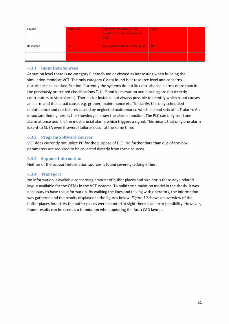
51
Layout Auto CAD Latest version with S60 not
available. No info on dedicated
rails.
Static.
Resources PD Not available. (OEMs and hangers) No.
Input Data Sources 6.3.1
At station level there is no category C data found or viewed as interesting when building the
simulation model at VCT. The only category C data found is at resource level and concerns
disturbance cause classification. Currently the systems do not link disturbance alarms more than in
the previously presented classifications T, U, P and K (starvation and blocking are not directly
contributors to stop alarms). There is for instance not always possible to identify which robot causes
an alarm and the actual cause, e.g. gripper, maintenance etc. To clarify, U is only scheduled
maintenance and not failures caused by neglected maintenance which instead sets off a T-alarm. An
important finding here is the knowledge in how the alarms function. The PLC can only send one
alarm at once and it is the most crucial alarm, which triggers a signal. This means that only one alarm
is sent to SUSA even if several failures occur at the same time.
Program Software Sources 6.3.2
VCT does currently not utilize PD for the purpose of DES. No further data than out-of-the-box
parameters are required to be collected directly from these sources.
Support Information 6.3.3
Neither of the support information sources is found severely lacking either.
Transport 6.3.4
No information is available concerning amount of buffer places and size nor is there any updated
layout available for the OEMs in the VCT systems. To build the simulation model in the thesis, it was
necessary to have this information. By walking the lines and talking with operators, the information
was gathered and the results displayed in the figures below. Figure 30 shows an overview of the
buffer places found. As the buffer places were counted at sight there is an error possibility. However,
found results can be used as a foundation when updating the Auto CAD layout.

52
The lack of update can be notice between Figure 31 and Figure 32. Figure 31 shows an older version
with color markings over areas which are different compared to the newer version displayed in
Figure 32. Figure 32 in turn shows dedicated tracks in the EOM roof-system. It also provides a visual
understanding of currently not updated areas in the Auto CAD, clearly related to the latest
manufacturing addition of body type S60, which are indicated with blue.
Inner Side Fixture
to Line-51
Inner Side Hanger
to Line-57
Roof to Line-
54
Outer Side
Fixture to Line-
57 Figure 31 Not updated Auto CAD drawing
Purple areas
are OEM
systems with
undedicated
side hangers
Blue areas are
OEM system
with
dedicated
side fixtures
Green area is
an OEM
system with
dedicated
roof fixtures
Figure 30 Gathered data related to buffer places in the EOM transportation system

53
Figure 32 Auto CAD drawing with dedicated transport tracks and added not updated areas
Inner Side Left Fixture to Line-57
Inner Side Left Hanger to Line-51
Side Left to Line-54
Side Right to Line-54
Inner Side Right Hanger to Line-52
V70/XC70 S60
S60
V60
S80
S60
V70/XC70
S80
V70
V60
S60
S80 V60
S60 V70/XC70
V70/XC70
V60
S80
S60
11-54-020
Direction of flow
V70 Body type New overhead monorail (OEM)
Elevator
Inner Side Right Fixture to Line-56

54

55
7 Input Data Management at VCT This chapter provides results based on the theory in section 2.2, Input data management, and goes
through the three headlines in the methodology process: Data collection, Data processing, and
Interfacing. The investigated data sources are CTview and SUSA. The first step described relates to
how the project utilized the manual data collection method according to Methodology A, see section
Data input methodologies. The second step was the processing which was made in MS Excel™ with
two tailored macros, programmed to fit SUSA and CTview. This enabled automatic processing. The
third step, interfacing, will be mentioned more briefly as it resulted to be out of the thesis
limitations.
7.1 Overview of the available formats What is interesting to notice is the lack of standardized format in use of date/time and station
number. This creates issues in the data processing step as the programming needs to be individually
customized. An overview of the time formats in the used systems can be seen in Table 9.
Table 9 Overview of the data format in the information sources at VCT
Processing
time
Transport time Cycle time Delta/
(Start to start)
Product Mix Down times
Origin CTView / TATS CTView CTView TATS CTView / TATS SUSA
Format SS,XX (number) SS.XX (text) SS.XX (text) SS (number)/
YYYY-MM-DD
HH:MM:SS
V60-V/H-M/U-
Var
(Text)
H:MM:SS
Processing Compare and
filter with
upper time
limit (90sec).
Substitute ”.”
for ”,” and use
VALUE formula
to change to
number format
Substitute ”.”
for ”,” and use
VALUE formula
to change to
number format
Filter with
upper time
limit and those
which contain a
failure. Used in
simulation
model.
Group variants
per car type
and filter
database using
DMAX, DMIN,
DAVERAGE,
DSTDEV
functions
Trim spaces,
format to time,
Change to
seconds by
multiplying by
hour, minute,
and seconds
Extracted Per product,
and per Robot,
filtered with
upper limit
Inconsistent
with
observations
Processing +
Transport
Missing
outbound
transport time
and
disturbances
Clean cycles per
product type
Maximum,
Minimum,
Mean, Std.
Deviation per
product type
Duration and
interval in
seconds [s]
Updated 2 weeks
(>~250 filtered
samples)
2 weeks
(>~250 filtered
samples)
2 weeks
(>~250 filtered
samples)
2 weeks
(>~250 filtered
samples)
Every variant
introduction or
3-6 months.
~1 year data to
have ~250
samples

56
7.2 CTview This section presents findings of the CTview system at VCT divided into three steps: collection,
processing and interfacing; as established in section 2.2.
Data Collection 7.2.1
Data regarding processing times could be collected either through CTView or using TATS Script tool.
For the purpose and time range decided for this study case, the TATS Script was used to collect
station cycle time data. A folder was created using the station identifier (e.g...//11-54-020/) for each
station. The MS Excel™ generated by the TATS Script was then saved inside the station folder using
the same station identifier and the prefix “CT” (e.g. CT1154202.xlsx).
Another file with the station identifier and the prefix “SUSA” was saved for each station of lines 54,
51 and 52 (e.g. SUSA1154020.xlsx). In these files, all kinds of disturbances registered in SUSA for the
same time period were stored.
Data Processing 7.2.2
A MS Excel™ file containing a Macro was developed in order to process the collected data for every
station. The Macro was programmed to extract delta times (start-to-start) from the previously
downloaded files and filter the data as mentioned previously on chapter2.2.3. This also contains a
Macro to allocate the failures and delete those cycles that contain a disturbance as explained in
section 4.3 and an additional one to filter out the cycles out of regular shifts hours. The result is a
table (e.g. Figure 33) containing the proposed cycle times (processing + transport times) for each
product type in each station. This times table can be easily copy-pasted into the simulation model
stations.
Figure 33 Cycle times after processing data.
Interfacing 7.2.3
No interfacing between applications was programmed but the use of a standardized spreadsheet for
all the stations allows the creation of an interfacing script in an easier way if further investigated.
7.3 SUSA This section presents findings of the SUSA system at VCT divided into three steps: collection,
processing and interfacing; as established in section 2.2.

57
Data Collection 7.3.1
The data collection process was performed manually. Disturbance data was gathered, in a folder
named based on line and station number, from week 1 to week 14 of 2014. This had to be done
manually as the data could not be downloaded in an MS Excel or other file format. An example of the
data gathered for station 11-51-010 can be seen in Figure 34. Each individual MS Excel™ workbook
was name according to the station name, e.g. S11_51_010. In all files the same headline as used in
SUSA was added with the information of what the columns contains, for instance “Radnr”,
“Maskinnr”, “Start störn”, etc.
Figure 34 Collected disturbance data for station 11-51-010 from SUSA
Data Processing 7.3.2
The information in SUSA was not presented as desired for simulation input and there was a need of
data processing to make format changes and calculations in order to get a usable representation. A
MS Excel macro was created, which automatically goes through all MS Excel workbooks in a folder. A
new file called InputData_ plus the workbook name was created for all workbooks. This means that it
is easy to separate SUSA-data with processed Input-data and that the name contains the station
code, e.g. “InputData_S11_51_010”. See Figure 35. The created excel shows headlines in Swedish
because SUSA is using Swedish. The very first row presents a text of the file used by the macro to
retrieve information. Only the first two, or potentially three, columns are intended to be used when
adding data into the simulation model. The data presented is in seconds to simplify usage.

58
Figure 35 Input data sheet in MS Excel for disturbances
Concerning the actual info transformation, “Start störn” (“start disturbance” in English) and “Stopp
störn” (“stop disturbance” in English) are timestamps directly taken from the source file
“S11_51_010”. This is done to provide transparency to the calculations performed. However, the
times have been cleaned from date and spaces to enable MS Excel calculations. By subtracting start
disturbance from stop disturbance the “Förlust” (“loss” in English) can be calculated. To make sure
the correct “Intervall” (“interval” in English) is calculated “Dag start” (“day start” in English) and “Dag
stopp” (“day stop” in English) is used as well as the number of week. Here the very same date-time
data has been taken from SUSA as for start and stop disturbance but the middle number for the day
is used instead.
Interfacing 7.3.3
No interfacing was done towards SUSA as it was found to be out of the project scope. However, the
created macro can be used for any SUSA file which could make a future investigated interface easier.
Disturbance Start: YYYYWWDHH:MM:SS

59
8 Discussion & Suggestions In this section several perspectives on the available and required data, presented in the results
section, will be further analyzed and discussed to reach a deeper understanding in topic. It will also
be discussed how these results can affect the creation of an automated DES model in future. The
order will be similar to the result chapter with required simulation model parameters and gap-
analysis, followed by more general suggestions connected to the created simulation model.
8.1 Required Simulation Parameters General required simulation parameters are brought up in the order presented in method and
results.
Processing time
Disturbances
Transportation
Product mix
Layout
Steering and process flow
Processing Time 8.1.1
In a utopian factory for a simulation expert, the processing times of the stations would contain
representative statistical distributions of a sufficient amount of cycles, which have not been affected
by changes in production or any kind of disturbance. The reason behind is that the disturbances
should be generated by the simulation model itself and have generate the same result as what
happens in reality. Nevertheless on VCT this is not the case because what is registered in the Virtual
Device as processing times is affected by disturbances of different kinds.
Processing times of the automatic stations in the Body Shop are normally logged by the PLC´s into
the Virtual Device and further calculated by the PLC´s logic at robot and at station level. The user can
query, through the OEE portal or directly from the TATS script, the times log of each of the stations.
In the process, the robots of a station may have different starting times in their processes in order to
avoid colliding with each other; they could also do extra non-value added activities like tip-dressing
or tool change before their processing time start. These extra activities depend on factors that are
not part of the operations, for example previous and current product variant, number of spot welds
since last tip-dress, etc. The frequency of these activities is irregular because they depend on the
product mix and the wear of the equipment.
After analyzing the logged information regarding processing times in the different systems, following
three main things will be pointed out as inadequate from the team perspective and should be
addressed. First, that there is an unclear definition of what is registered as “processing time” in the
Virtual Device. The processing times should vary depending on the product variant that is being
processed and even within the same kind of product a minor variability is expected, which could be
considered as negligible. However it is unclear when a tip-dress check and actual tip-dress is done,
and whether tool change or other preparatory action is included in the registries or not. Second, the
processing times get disturbed by the alarms within the station. Some robot registers have a very
long time since an alarm, read by the PLC, is triggered and this affects somehow the processing time
calculation overall. There have been detected cases when the processing time is longer than the

60
cycle time (start-to-start), which is logically impossible. Third, that there is an unclear register of the
start and end of the processing time timestamps against transportation times. It was assumed that
the processing time would be triggered by the first operating robot and stopped by the last one but it
has been observed that is not always the case. Also it is important to note that the “processing
times” of the station registered in VD is the complement of the transport system interval within the
start-to-start interval.
What has been proposed as trustful times are the Cycle time and start of failure timestamps at the
VD. The team considers cycle times as truth since they only involve the income of a new product into
a station and alarms can be neglected. Also disturbances start timestamps can be considered as truth
because even if alarms overlap each other the first one will have to be cleared before a new product
can be processed. Therefore the process of clean cycle times is supported by allocating the start
timestamps of the failures from SUSA registers between the cycle times’ timestamps and filtering the
ones that do not have any alarm in between. This filtering process will result in cycle times that
contain only processing and transport times.
Disturbances 8.1.2
The quality of the disturbance data found in SUSA can be considered insufficient to be used in a
simulation model. The disturbance start time is correct but the end time has been observed to be
incorrect. When a disturbance occurs the PLC sends out a signal which continues throughout the
complete cycle. The full disturbance time detected is thus the actual disturbance time plus the rest of
the processing time. This is the case no matter when in the processing cycle the failure occurs. The
data can therefore not be considered reliable. Another quality issue is during circumstances when
one alarm overshadows another alarm. There can be several failures at once but only on failure
alarm will be detected by SUSA. The alarm classification can therefore not be completely trusted for
all situations. It does not directly influence the ability to build a simulation model but affects the
reading of the simulation results.
There are daily situations where the operator zeroes out the time of failure duration under the
headline losses (“förlust” in Swedish). This happens when the station is blocked or starving due to
other disturbances in the flow. The operator uses this time to do maintenance or fixing a smaller
problem, and it is the opening of the door which triggers an alarm that is recorded in SUSA. The time
is thus not adding to the stoppage of the line which means it is not a direct production loss. However,
by using this system important statistics get lost which can be necessary in order to predict future
maintenance needs and failures, as simulation data input used by the simulation builder.
Availability is another option to using disturbance intervals and duration. Availability can be
calculated from the real time data if necessary steps of cleaning the data are taken to achieve
enough quality, as discussed previously. By storing the availability in Process Designer it can more
easily be accessed, since the intuitive location for employees would be to search for this type of
information here. Line-builders can add this information directly in distributed the Line-model and
the time consuming task of retrieving the data from them can thus be eliminated. The issue with this
solution is that if availability is changed for a specific type of gripper it has to be changed for each
single one of these grippers in PD. A way around the updating issue would be to have the availability
for each type of gripper, robot, tip weld tool etc. in a separate sheet. When the sheet is updated it

61
should automatically update all resources in the PD with the same name. A standardized naming
procedure would therefore be extremely important.
Transportation 8.1.3
For the transportation system with conveyors, elevators, turn-tables etc. there is a lot of information
missing. The main problem here is general lack of documented information in a standardized
manner. For the investigated lines there was not found documentation on: empty buffer places,
indications of body-type-dedicated transport, number of hangers used or speed. Transport times are
not registered in any data source but needs to be calculated as an average in how long it takes for
one inner-side to travel to the position where it is merged with the matching outer-side.
Line-52, producing right-hand-sides, are having problems with incoming EM-cards on the hanger not
being read properly. The wrong body-type can be directed by the roof steering system into a buffer
space for a different body-type. When the inner-side enters station 11-52-060 the line stops. This
causes problems which are not easily detected and in need of manual support by the Line-
maintenance responsible. For instance, a V70/XC70 carrier can be directed to the V60 buffer. Other
failures related to the PLC and sensor reading in relation to the ordering system has also been found,
but the direct cause has not been detected. The main issue is the future impact these problems
would have on an automated model since the quality of data can be viewed deficient. The DES
model would not generate trustworthy results.
One aspect which could influence the possibility of creating an automated DES model in the future
would be to name the transport systems in the same systematic structure as the lines are named.
There are two prime reasons behind this. Firstly, as it is now the lack of name leads to confusion and
potential risk of misunderstandings. For instance, between inner sides and outer sides there is EOM
transportation, but there is also EOM transportation to inner sides and from outer sides. To have a
name on each of these transportation systems would facilitate efficient knowledge exchange.
Secondly, a naming procedure would bring importance to the transportation system. In the current
VCT body shop factory very little consideration is done to transportation. Focus lies within direct
value adding procedures and stations. However there is great potential in addressing transportation
issues such as buffers and logic steering. For instance transportation can delimit throughput time if
product mix is changed. Overall time efficiency can be improved by directing efforts to handling of
the transportation systems.
A DES model can only give assistance here if there is enough available data for the transportation
systems, which there is currently not. To summarize, the transportation system information needs to
be added somewhere.
Product mix 8.1.4
The product mix is another reason to put focus on the EOM transportation systems on the second
floor, between processing lines. The simulation model and investigations of the chosen production
scope showed indications on process output changes when changes in the product mix. The reason is
the size and product dedication of the buffer places and how locking effects can occur due to this.
There are limitations in the system flexibility when it comes to product mix which can reduce or
enhance output drastically.

62
Layout 8.1.5
Updates of the layout have not been done in the AutoCAD™ files for the conveyor systems in the
roof, which was used in the thesis. There have also been misunderstandings related to the layout as
not all versions had the latest update. However, the thesis did not have access to all the information
and had to trust information sources in providing the AutoCAD™ files.
Steering and Process Flow 8.1.6
Steering and process flow became clearer only after several sessions of walking-the-line. The TATS
system gives some indication for the floor process but transportation, roof and side lines are more
unclear. The Mitsubishi PLC code was investigated but did not provide any clarity because the
program is old and badly commented on. This yielded in assumptions from the thesis team in order
to simulate the designated production area. However, the PLC signals should be able to send out
timestamps for the transportation system as well. Therefore further investigation or redirecting
these types of questions to a more knowledgeable person is advised.
8.2 Simulation Model A good measure of quality of data proposed is to look into two aspects: the availability of data
according to its category and the effort of processing it. Regarding availability of data it is important
to know how often does the simulation input parameters need to be updated and how much a
change could affect the process. The distribution fit is a statistical description of how likely is it for
the data to be compared to a statistical distribution. Nevertheless the quality of the data should not
be confused to the likelihood of the data with a statistical distribution, the quality of the data should
be validated against the sources of it, making sure that the correct data is registered and the amount
of further processing effort that need to be done on it in order to make it usable for the simulation
modeler.
8.3 Information mapping The way in which the team proceeded to look for the information required to build the simulation
model lead to different challenges to get the information. Some of the information sources resulted
to be unusable and unreliable, thus making it difficult to understand the steering of performance of
the station resources. When constructing the simulation model the team encountered with the
challenge of having an old generation production line that has not been maintained in its virtual
documents. Many of the layouts, Process Designer processes and documentation are not updated
and contain mayor faults to be considered as complete.
8.4 Suggestions To enable the StreaMod project the following headlines are suggested to be looked through in order
to fill the gaps of lacking information and data. Direct propositions are suggested below together
with more general improvements which can be implemented.
Processing times: 8.4.1
Define what builds up the processing time and what should be considered as preparatory or
setup actions (tip-dress, tool change).
Register the times for each of the robots in a clear way. Take advantage of the different
operation trees available at Process Designer to register what the planned time is, use the
resource tree to store information about statistical representations of the process if the

63
attributes defined by default are constant or create customized attributes to include
statistical data of the process.
Standardize format, decimal spaces and decimal separator.
Increase the availability of historical data in all the stations. Currently a small portion of the
available data is visible in OEE portal, 45 days is visible in the TATS script and other in TAP.
Be aware of VD quality of data within Axxos implementation.
Disturbances: 8.4.2
The authors propose the use of standardized operator comments in combination of
providing the operators with sufficient information to enable an understanding on why the
standardization is necessary and should be kept.
Store availability in Process Designer organized by object. Information is then easier found by
more people within the organization as the storage location is intuitive. Updates can be
necessary over time as the equipment is used and make it a standardized procedure to have
this added by the supplying line-builders.
Transportation: 8.4.3
Name the overhead monorail transportation systems between lines to avoid confusion, bring
importance, and enable a future automatic DES.
Enable the StreaMod project by adding time stamps when entering and leaving an overhead
monorail transportation system.
Layout: 8.4.4
Update existing AutoCAD files with the added transportation conveyor systems in the roof
for the side lines.
Add indications to buffer places in existing AutoCAD files.
Steering and Process Flow: 8.4.5
Store logic of lines with stations in an understandable way.

64

65
9 Conclusion The StreaMod project demands data with sufficient quality to enable a future automatic simulation
model creation.
9.1 Main changes What needs to be done in terms of data quality are mainly the following (see Figure 36):
Steering logic: Clarification needed in general. Documentation of what logic and conditions
drive the interactions between stations, transport systems and alarms management. Also
definition on material flow and product type specific processes.
Processing time: From the timestamp of a body entering a station, where the fixtures start
operating, to timestamp where the processing is completed. Thus the end timestamp needs
to be adjusted to match this and not until the next station is ready – latter would be a
scenario of blocking.
Disturbance: The time for disturbance stop needs to be adjusted to the actual stop, and not
the stop of the entire processing.
Transportation: times between lines need to be logged. Perhaps in CTview as a station.
Figure 36 Sand cone model with main priorities displayed bottom-up
9.2 General changes To enhance the performance and lower manual work time there are additional beneficial parameters
to decipher. Furthermore, in the future maintenance and energy utilization are likely two aspects,
which will become valuable to investigate with the help of simulation modeling. For mentioned
reasons the following data quality concerns need to be looked at:
Transportation equipment should be updated every second week. Make it a standardized
event.
Added Between Line Transportation Times
Accurate Disturbance Stop Time
Accurate Processing Times
Steering Logic Displayed Clearly
66
Buffer capacity should be stored in AutoCAD™ and updated whenever a change in the
production process is made, e.g. introduction of new body type.
Dedication of rails should be stored – perhaps together with steering logic.
Energy usage can be calculated from processing type and duration.
Finally, cause identification can be addressed at resource level by adding the different
robotic failures to SUSA, thereby achieving better simulation results and maintenance
control.
9.3 Suggestions for the future From the results and based on the conclusion it is suggested that future thesis work should
preferably, to benefit the StreaMod project, be in the following areas:
Data quality in the production with time studies to define errors and create standardization
for timestamps and other information.
Alarm management and disturbance management.
In combination with above, PLC debugging and creation of new PLC standard.

67
References Banks, J. 1998. Handbook of Simulation – Principles, Methodology, Advances, Applications, and
Practice. John Wiley & Sons.
Bergman, B., and Klefsjö, B. 2010, Quality from Customer Needs to Customer Satisfaction. Third
edition. Studentlitteratur.
Bergmann, S., Stelzer, S. & Strassburger, S. 2011, "Initialization of simulation models using CMSD",
IEEE, , pp. 2223.
Cavazzuti, M. 2013, "Design of Experiments" in Springer Berlin Heidelberg, Berlin, Heidelberg, pp. 1-
10 and 13-42.
Chung, C.A. Donaghey, C.E. 2004, Simulation modeling handbook: a practical approach, Chapter 5,
CRC Press Inc, Boca Raton, Fla; London
Davenport, T.H., Prusak, L. 1998. Books24x7, I. & Books24x7 - ITPro & BusinessPro (e-book
collection), Working knowledge, Harvard Business School Press, Boston, Mass
Fournier, J. 2011, "Model building with Core Manufacturing Simulation Data", IEEE, , pp. 2214.
Goos, P., Jones, B. Books24x7 - EngineeringPro (e-book collection) 2011, Optimal design of
experiments: a case study approach, Wiley, Chichester, West Sussex, U.K.
Leemis, L. 2004. Building incredible input models. In Proceedings of the 2004 Winter Simulation
Conference, ed. R. G. Ingalls, M. D. Rossetti, J. S. Smith and B. A. Peters, 29-40. Washington, D.C.
Liker, J.K Meier, D. (2006) The Toyota Way Fieldbook: A practical guide for implementing Toyota’s
4Ps. Mcgraw-Hill Companies Inc.
Microsoft. http://office.microsoft.com/en-us/excel/. 2014-05-30
Montgomery, D. C. (2000). Design and analysis of experiments (5th ed.). New York: Wiley.
Moon, Y. B., Phtak, D. 2005. Enhancing ERP system’s functionality with discrete event simulation,
Industrial Management & Data Systems, 105:1206-1224.
Musselman, K. 1994, "Guidelines for simulation project success", Society for Computer Simulation
International, WSC '94 Proceedings of the 26th conference on Winter simulation, pp. 88-95.
Pedgen, D. C.; Shannon R. E.; & Sadowski, R.P. Introduction of Simulation using Siman. 2 Ed. U.S.A.:
McGraw-Hill, 1995.
Perera, T., Liyanage, K. 2000. Methodology for rapid identification of input data in the simulation of
manufacturing systems. Simulation practice and Theory 7:645-656.
Perrica, G., Fantuzzi, C., Grassi, A., Goldoni, G., and Raimondi, F.2008. Time to Failure and Time to
Repair Profiles Identification. In Proceedings of the 5th FOODSIM conference. Dublin, Ireland.
Robertson, N., Perera, T. 2002. Automated data collection for simulation?. Simulation Practice and
Theory 9:349-364.
68
Robertson, N., Perera, T. 2001, Automated data collection for simulation? Simulation Practice and
Theory, pp. 349-364.
Robinson, S. 2004. Simulation: The Practice of Model Development and Use.Chichester: John Wiley &
Sons.
Robinson, S., Bhatia, V. 1995.Secrets of successful simulation projects. In Proceedings of the 1995
Winter Simulation Conference, ed. C. Alexaopoulus, K. Kang, W. R. Lilegdon and D. Goldsman, 61-67.
Arlington, Virginia.
Salem, R., Boussaïd. O., Darmont, J. 2013. Active XML-based Web data integration. Inf Syst Front (15),
pp. 371-398. Springer Science+Business Media New York.
Sargent, R.G. 2010. Validation and verification of simulation models. In: Proceedings of the 2010
Winter Simulation Conference, pp.166-183.
Slack, N. Lewis, M. (2011) Operations Strategy. Third edition. Harlow, Essex: Pearson Education
Limited.
Skoogh, A., Johansson, B. 2009. Mapping of Time-Consumption During Input Data Management
Activities, Simulation News Europe, 19, 39-46
Skoogh, A., Johansson, B. & Stahre, J. 2012, "Automated input data management: evaluation of a
concept for reduced time consumption in discrete event simulation",
Skoogh, A., B. Johansson. 2008. A Methodology For Input Data Management In Discrete Event
Simulation Projects. Proceedings of the 2008 Winter simulation Conference, pp. 1725-1737.
Skoogh, A., Johansson, B. 2007. Time-consumption analysis of input data activities in discrete event
simulation projects. In Proceedings of the 2007 Swedish Production Symposium. Gothenburg,
Sweden.
Williams, E.J. & Ulgen, O.M. 2012, "Pitfalls in managing a simulation project", IEEE, pp. 1.

I
Appendix A
OEE for production simulation flow purposes
About OEE Portalen
The OEE Portal is a visualization tool for the TAP database in which the user can extract and visualize
information about different operational times at a certain production area. The data can be exported
to .CSV, .XLS, or .XML format for further processing. Depending on the station, the data that can be
collected from the database include cycle start timestamp in “YYYYWWD HH:MM:SS” format, station
processing time, Product variant, and status. Sometimes the station also collects the processing time
for each robot separately and transportation time.
Figure 37 CTview interface in OEE
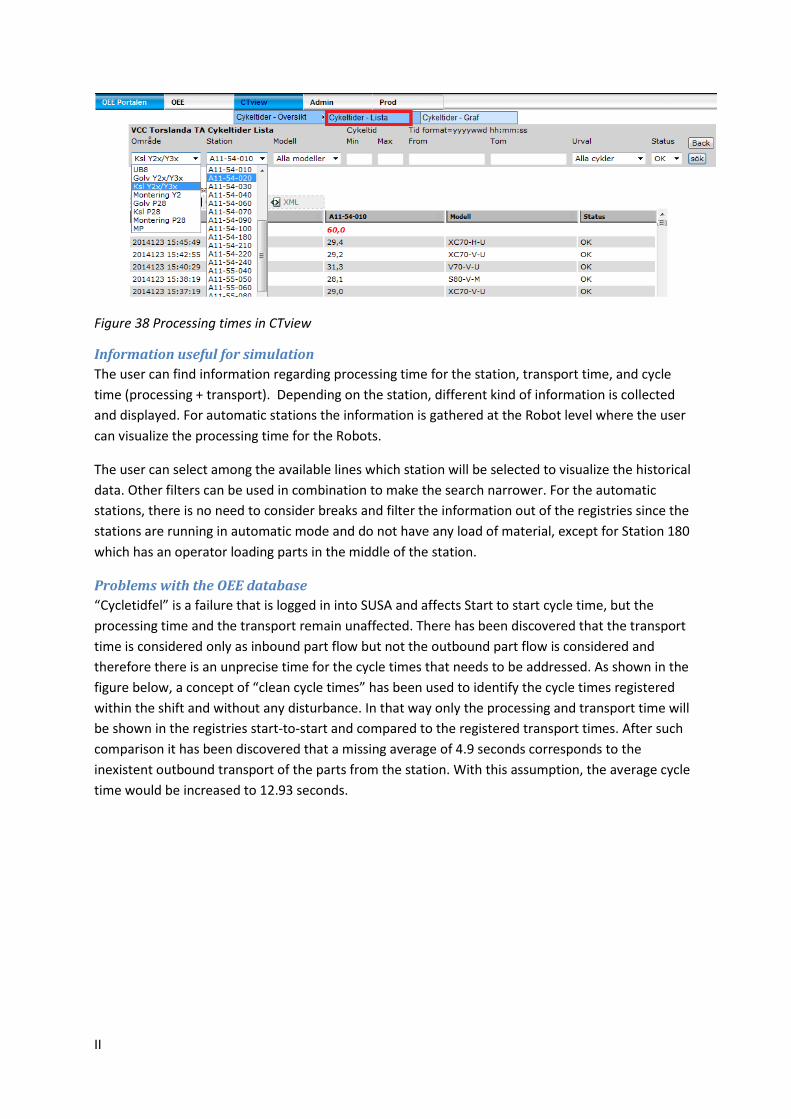
II
Figure 38 Processing times in CTview
Information useful for simulation
The user can find information regarding processing time for the station, transport time, and cycle
time (processing + transport). Depending on the station, different kind of information is collected
and displayed. For automatic stations the information is gathered at the Robot level where the user
can visualize the processing time for the Robots.
The user can select among the available lines which station will be selected to visualize the historical
data. Other filters can be used in combination to make the search narrower. For the automatic
stations, there is no need to consider breaks and filter the information out of the registries since the
stations are running in automatic mode and do not have any load of material, except for Station 180
which has an operator loading parts in the middle of the station.
Problems with the OEE database
“Cycletidfel” is a failure that is logged in into SUSA and affects Start to start cycle time, but the
processing time and the transport remain unaffected. There has been discovered that the transport
time is considered only as inbound part flow but not the outbound part flow is considered and
therefore there is an unprecise time for the cycle times that needs to be addressed. As shown in the
figure below, a concept of “clean cycle times” has been used to identify the cycle times registered
within the shift and without any disturbance. In that way only the processing and transport time will
be shown in the registries start-to-start and compared to the registered transport times. After such
comparison it has been discovered that a missing average of 4.9 seconds corresponds to the
inexistent outbound transport of the parts from the station. With this assumption, the average cycle
time would be increased to 12.93 seconds.

III
Appendix B
Using SUSA for production flow simulation purposes
About SUSA
SUSA is an internally developed application that logs all the downtimes information of the production
lines at the TA shop. This system is used by simulation and maintenance engineers to track and
follow up disturbances at the different stations. It collects and filters the data from the “Virtual
Device” database, which receives the PLC´s raw data from the production floor.
Warnings about SUSA
The empirical studies made by the team at one of the stations (11-54-020) suggest that the log of
failures into SUSA is not as reliable as expected regarding duration and mode of failure. In the case
that a failure occurs in a resource of a station, a first alarm will be triggered and its timestamp will be
registered in SUSA. The duration of the failure is observed to be from the start of the failure until the
end of that complete cycle, including outbound transportation of the product. In case that a second
resource fails SUSA will only register the first cause of alarm and ignore all consequent alarms until
the end of the current cycle.
Figure 39 Logged signals in SUSA
It is also important to note that the operator has the possibility to declare when a disturbance
register relates to a production loss or not. In case the disturbance does not affect the production
then the operator would normally delete the time out of the “förlust” (loss) field. The operator can
comment out the disturbances too but there is not a clear definition of when a comment
To open SUSA go into the following link:
http://wwwapp.gothenburg.vcc.ford.com/prodrapp/tclient/javaplugin.htm
To work with VCT body shop click on “SUSA via TClient TA”

IV
To enter into the system log in anonymously (“Anonym login”):
Start the LOGGAR application.

V
In this application the user can search and filter all the down time registers for a specific line or
station. The registers can be then visualized in a table that contains the machine number, start and
stop timestamp of the down time, shift, down time duration (stopptid), down time duration that can
be considered as production loss (förlust) , system´s failure description, cause, comment editable by
the operator, and others not as relevant for this thesis purpose.
It is important to mention that the timestamps of start and stop of failures are in the following
format:
“YYYY WW D HH:MM:SS”, where YYYY is the year, WW the week of the year, D is the day of the week
(e.g. 1= Monday, 6=Saturday), and HH:MM:SS the actual timestamp in that day.
After the results are displayed in the screen they can be copied and pasted on a conventional
spreadsheet for further data processing or documentation purposes.

VI
To narrow you search the user can use the following available options:
Maskinnr – Number of machine or station. In this field the number of the station can be added. The
first 2 digits represent the site or facilities in Volvo Cars (For example, 11=Torslanda A-shop 1 or TA1,
13=BSO Y2X, 14= TA2, 15=UB8). The second 2 digits field represent the line number (For example,
54= Framing, 55= Respot). The next 3 digits are the number of the station (for example 020 = Framing
station, 010 = Ringframe).
Felltyp – Type of failure. Describes the mode or reason of failure. K= Quality related, L= Related to
the station, M=Material (not used), P=Related to Personnel mostly when breaking through a safety
area. T= Technical Failure caused by the equipment or process in the station (most common and
relevant).
Waiting (VS- väntestopp) and blocked (FS- följdstopp) times are also registered in SUSA as down
times even if they are consequence of the upstream and downstream production system. A good
filter to visualize only station related down times is STP (K+L+M+P+T).

VII
A common way to see all the available information in SUSA is by setting the attribute “Urval”
(selection) to “Rubbet” (whole lot) must be selected:
The system has a restriction regarding historical data. The user can display maximum 999 registries
(Rader) in the screen at once, for a maximum time lapse period of 35 days. The user can advance to
the next page of registries by pressing F8 key. These 35 days interval can be adjusted to prior dates
following the specified previous format “YYY MM D” & “HH:MM”. The earliest available data is
around week 37 of 2011.

VIII

IX
Appendix C
TATS - (TA Terminal Services)
TATS Script is an information source used by the thesis team to collect the data regarding processing
and cycle time for each of the stations involved in the study case. It has been used because it is the
information source that provides the largest amount of historical information of timestamps that are
collected by the Virtual Device. TATS Script runs over a website developed internally by VCT in which
information about the Virtual Device and production equipment can be displayed. It is one of the
most used resources for manufacturing engineers at VCT to monitor the activity of the current
production and contains relevant links to other frequently visited internal websites.
In order to run the TATS Script, the user has to clic on “CT View to Excel” under the “Buffert” menu,
this action will result in the generation of an excel file that contains the information of a default
station. In order to use this Script and access the information of other stations, the user has to
manually change the URL address in the internet browser and write the number ID of that specific
station. Figure XX shows the URL address segments that the user has to adjust to generate the
desired excel file. Then the user can download the generated excel file from the link displayed on the
website.
Figure 40. Access to TATS Script tool.
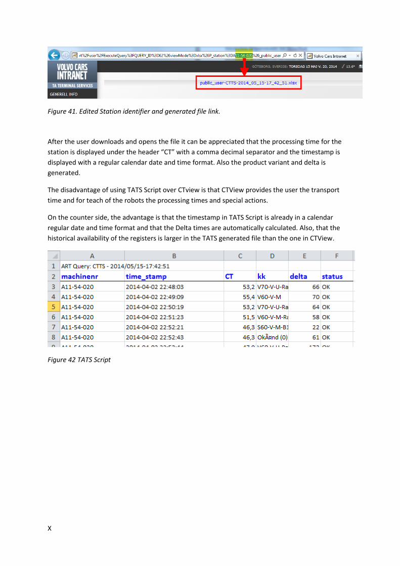
X
Figure 41. Edited Station identifier and generated file link.
After the user downloads and opens the file it can be appreciated that the processing time for the
station is displayed under the header “CT” with a comma decimal separator and the timestamp is
displayed with a regular calendar date and time format. Also the product variant and delta is
generated.
The disadvantage of using TATS Script over CTview is that CTView provides the user the transport
time and for teach of the robots the processing times and special actions.
On the counter side, the advantage is that the timestamp in TATS Script is already in a calendar
regular date and time format and that the Delta times are automatically calculated. Also, that the
historical availability of the registers is larger in the TATS generated file than the one in CTView.
Figure 42 TATS Script

XI
Appendix D
Results of the Simulation Model
The simulation model was run for a period of 20 days. The expectation of the data collection and
processing was to have only clean cycle times that contain only processing and transport times,
excluding the disturbances in the system. This expectation was not accomplished since the resultant
filtered times, as explained in section Error! Reference source not found., still contained samples
asting much longer than the designed cycle time at planning stages. This result arised several
questions regarding the alarm management at the PLC´s and the reliability of the logged disturbance
timestamps.
In the first experiment, for practical purposes the thesis team decided to feed the simulation model
with the processed cycle times as triangular distributions and failures as empirical functions for the
lines 51, 52 and 54. The result was significantly lower than the actual production at VCT, invalidating
the simulation model results. Figure XX shoes that the throughput for this experiment is around 25
jobs per hour (JPH) and around 600 throughput per day.
Figure 43. Output statistics
A second experiment was designed based on two assumptions. First, that the failures registers are
unreliable and that disturbances are embedded in the processed cycle times. Second, that the
processed cycle times can fit into Triangular and Normal Distributions since they are automated
processes. The experiment was designed with two levels. The first level of the experiment was using
as Processing times the collected information with a triangular distribution function and the second
level was using a normal distribution function. The days were considered as full 24 hour working
periods and no failures have been setup in any of the stations. Figure 44 shows that the simulation
outputs in average 46.44 jobs per hour for a normal distribution and 43.19 jobs per hour for a
triangular distribution with a confidence level of 90%.
Figure 44. Second experiment simulation results
These previous results are more likely to be a valid representation of the system since a regular 2
shift working day (06:30 to 00:00 hrs) has a throughput of around 720 car bodies.
Some other interesting outputs from the simulation model for manufacturing engineers were uneven
utilization of resources. Left and right BSI lines had different amount of fixture changes to cope with
the product mix. Also the amount of dedicated fixtures for each product type was not optimal. Figure
45 and Figure 46 show that one S60 fixture could be taken away from the system but is not the same
case for the other product types.

XII
Figure 45. BSI -LH buffer utilization.
Figure 46. BSI -RH buffer utilization.