5/9/2012

1

Data-Flow Graph Model

EE216B: VLSI Signal Processing

Prof. Dejan Marković ee216b@gmail.com

Iteration

Iterative nature of DSP algorithms

– Executes a set of operations in a defined sequence

– One round of these operations constitutes an iteration

– Algorithm output computed from result of these operations

Graphical representations of iterations [1]

– Block diagram (BD)

– Signal-flow graph (SFG)

– Data-flow graph (DFG)

– Dependence graph (DG)

Example: 3-tap filter iteration

– y(n) = a·x(n) + b·x(n−1) + c·x(n−2), n = {0, 1, …, ∞}

– Iteration: 3 multipliers, 2 adders, 1 output y(n)

[1] K.K. Parhi, VLSI Digital Signal Processing Systems: Design and Implementation, John Wiley & Sons Inc., 1999.

11.2

5/9/2012

2

Block Diagram Representation

mult add delay/reg

y(n) = a·x(n) + b·x(n−1) + c·x(n−2), n = {0, 1, …, ∞}

x(n)

a b c

y(n)

Block diagram of 3-tap FIR filter

+ z−1

z−1 z−1

+ +

11.3

Signal-Flow Graph Representation

constant multiplication (a) or register (z−1) on edges

edge

j k

Network of nodes and edges

– Edges are signal flows or paths with non-negative # of regs

● Linear transforms, multiplications or registers shown on edges

– Nodes represent computations, sources, sinks

● Adds (> 1 input), sources (no input), sinks (no output)

a / z−1

3-tap FIR filter signal-flow graph z−1 z−1

a b c

y(n)

x(n)

source node: x(n) sink node: y(n)

11.4

5/9/2012

3

Transposed SFG functionally equivalent

– Reverse direction of signal flow edges

– Exchange input and output nodes

Commonly used to reduce critical path in design

z−1 z−1

a b c

y(n)

x(n)

Transposition of a SFG

z−1 z−1

a b c

x(n)

y(n)

Original SFG

Transposed SFG

tcrit = 2tadd + tmult

tcrit = tadd + tmult

11.5

Different Representations

z−1 a

y(n) x(n)

SFG

x(n) y(n)

a BD

A

B

(1)

(2)

x(n) y(n)

DFG

Block Diagram (BD)

– Close to hardware

– Computations, delays shown through blocks

Signal-flow Graph (SFG)

– Multiplications, delays shown on edges

– Source, sink, add are nodes

Data-flow Graph (DFG)

– Computations on nodes A, B

– Delays shown on edges

– Computation time in brackets next to the nodes

D

+

z−1

+

11.6

5/9/2012

4

Data-Flow Graphs

Graphical representation of signal flow in an algorithm

x1(n) x2(n)

y(n)

v1 v2

v3

v4

e1 e2

e3 Z-1 D

Nodes (vi) → operations (+/−/×/÷)

Registers → Delay (D)

Node-to-node communication,

edges (ei)

Iterative input

Iterative output

Registered edge, edge-weight = # of regs

Edges define

precedence constraints b/w operations

+

z−1

11.7

Formal Definition of DFGs

A directed DFG is denoted as G = <V,E,d,w>

• V: Set of vertices (nodes) of G. The vertices represent operations.

• d: Vector of logic delay of vertices. d(v) is the logic delay of vertex v.

• E: Set of directed edges of G. A directed edge e from vertex u to vertex v is denoted as e:u → v.

• w(e) : Number of sequential delays (registers) on the edge e, also referred to as the weight of the edge.

• p:u→ v: Path starting from vertex u, ending in vertex v.

• D: Symbol for registers on an edge.

e1: Intra-iteration edge e3 : Inter-iteration edge

w(e1) = 0, w(e3) = 1

x1(n) x2(n)

y(n)

v1 v2

v3

v4

e1 e2

e3

Z-1

D

+

11.8

5/9/2012

5

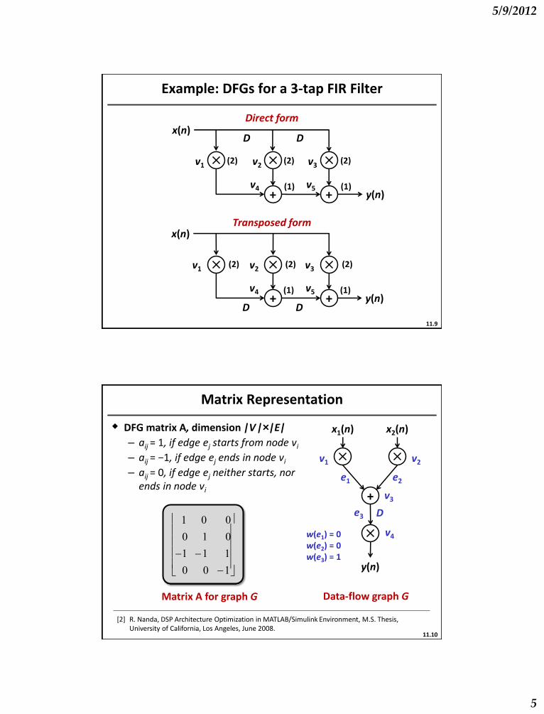
Example: DFGs for a 3-tap FIR Filter

Direct form

Transposed form

x(n)

v1

y(n)

v2 v3 (2) (2) (2)

v4 (1) (1) v5

D D

x(n)

v1

y(n)

v2 v3 (2) (2) (2)

v4 (1) (1) v5

D D

+ +

+ +

11.9

Matrix Representation

DFG matrix A, dimension |V |×|E|

– aij = 1, if edge ej starts from node vi – aij = −1, if edge ej ends in node vi

– aij = 0, if edge ej neither starts, nor ends in node vi

w(e1) = 0 w(e2) = 0 w(e3) = 1

1 0 0

0 1 0

1 1 1

0 0 1

Matrix A for graph G Data-flow graph G

x1(n) x2(n)

y(n)

v1 v2

v3

v4

e1 e2

e3

Z-1

D

+

[2] R. Nanda, DSP Architecture Optimization in MATLAB/Simulink Environment, M.S. Thesis, University of California, Los Angeles, June 2008.

11.10

5/9/2012

6

Matrix Representation

Weight vector w

– dimension |E |×|1|

– wj = w(ej), weight of edge ej

Pipeline vector du

– dimension |E|×|1|

– duj = pipeline depth of source node v of edge ej

0

0

1

Vector w Data-flow graph G

0

0

1

Vector du

x1(n) x2(n)

y(n)

v1 v2

v3

v4

e1 e2

e3

Z-1

D

+

11.11

Simulink DFG Modeling

Drag-and-drop Simulink flow

Allows easy modeling

Predefined libraries contain DSP macros

– Xilinx XSG

– Synplify DSP

Simulink goes a step beyond modeling macros

– Functional simulation of complex systems possible

– On-the-fly RTL generation through Synplify DSP Synplify DSP block library

11.12

5/9/2012

7

DFG Example

QAM modulation and demodulation

Combination of Simulink and Synplify DSP blocks

11.13

Summary

Graphical representations of DSP algorithms

– Block diagrams

– Signal-flow graphs

– Data-flow graphs

Matrix abstraction of data-flow graph properties

– Useful for modeling architectural transformations

Simulink DSP modeling

– Construction of block diagrams in Simulink

– Functional simulation, RTL generation

– Data-flow property extraction

11.14

5/9/2012

8

Architecture Transformations

DFG Realizations

Data-flow graphs can be realized with several architectures

– Flow-graph transformations

– Change structure of graph without changing functionality

– Observe transformations in energy-area-delay space

DFG Transformations

– Retiming

– Pipelining

– Time-multiplexing/folding

– Parallelism

Choice of the architecture

– Dictated by system specifications

11.16

5/9/2012

9

Retiming

Registers in a flow graph can be moved across edges

Movement should not alter DFG functionality

Benefits

– Higher speed

– Lower power through VDD scaling

– Not very significant area increase

– Efficient automation using polynomial-time CAD algorithms [2]

[1] C. Leiserson and J. Saxe, "Optimizing synchronous circuitry using retiming,“ Algorithmica, vol. 2, no. 3, pp. 211–216, 1991.

[2] R. Nanda, DSP Architecture Optimization in MATLAB/Simulink Environment, M.S. Thesis, University of California, Los Angeles, 2008.

[1]

11.17

Retiming

Register movement in the flow graph without functional change

w(n) = a∙y(n − 1) + b∙y(n − 3) y(n) = x(n) + w(n − 1) y(n) = x(n) + a∙y(n − 2) + b∙y(n − 4)

x(n)

y(n)

D

3D

D

w(n − 1)

a b

w(n)

x(n)

y(n)

D

3D

D

a b

v(n)

D * Retiming moves

Retimed Original

×

+

×

+

×

+

×

+

v(n) = a∙y(n − 2) + b∙y(n − 4) y(n) = x(n) + v(n) y(n) = x(n) + a∙y(n − 2) + b∙y(n − 4)

11.18

5/9/2012

10

Retiming for Higher Throughput

Register movement can shorten the critical path of the circuit

x(n)

y(n)

D

3D

D

w(n − 1)

a b

w(n)

x(n)

y(n)

D

3D

D

a b

v(n)

D

×

+

×

+

×

+

×

+

Retimed Original

(1) (1)

(2)* (2)

(1) (1)

(2)* (2)

*Numbers in brackets are combinational delay of the nodes

Critical path reduced from 3 time units to 2 time units

Critical path

11.19

Retiming for Lower Power

x(n)

y(n)

D

3D

D

w(n − 1)

a b

w(n)

x(n)

y(n)

D

3D

D

a b

v(n)

D

×

+

×

+

×

+

×

+

Retimed Original

(1) (1)

(2) (2)

(1) (1)

(2) (2)

Exploit additional combinational slack for voltage scaling

Timing slack = 0 Timing slack = 1

Desired throughput: 1/3

11.20

5/9/2012

11

Retiming Cut-sets

Manual retiming approach

– Make cut-sets which divide the DFG in two disconnected halves

– Add K delays to each edge from G1 to G2

– Remove K delays from each edge from G2 to G1

x(n)

y(n)

D

3D

D

a b x(n)

y(n)

2D

D

a b

D

× ×

+

×

+

×

+

G1

G2

Cut-set

G1

G2

Cut-set

e1

e2

e3 e4

e1

e2

e3 e4

K = 1 (a) (b)

D

+

11.21

Mathematical Modeling

Assign retiming weight r(v) to every node in the DFG

Define edge-weight w(e) = number of registers on the edge

Retiming changes w(e) into wr(e), the retimed weight

x(n)

y(n)

D

3D

D

a b 4

1

3

2

e2 e3

e4 e5

e1

r (1) r (2)

r (4) r (3) w(e1) = 1 w(e2) = 1 w(e3) = 3 w(e4) = 0 w(e5) = 0

wr (e) = w(e) + r (v) – r (u)

Retiming equation

[2] R. Nanda, DSP Architecture Optimization in MATLAB/Simulink Environment, M.S. Thesis, University of California, Los Angeles, 2008.

[2]

11.22

5/9/2012

12

Path Retiming

Number of registers inserted in a path p: v1→ v2 after retiming

– Given by r(v1) − r(v2) – If r(v1) − r(v2) > 0, registers inserted in the path – If r(v1) − r(v2) < 0, registers removed from the path

x(n)

y(n)

D

3D

D

a b x(n)

y(n)

2D

D

a b

D

4

1

3

2

4

1

3

2

D

wr(p) = w(p) + r(4) − r(1) = 4 − 1 (one register removed from path p)

r(1) = 1 r(2) = 1

r(4) = 0

r(3) = 0

Path p:1→4 Path p:1→4

11.23

Optimization Methods (Scheduling & Retiming)

5/9/2012

13

Mathematical Modeling

Feasible retiming solution for r(vi) must ensure

– Non-negative edge weights wr(e)

– Integer values of r(v) and wr(e)

x(n)

y(n)

D

3D

D

a b 4

1

3

2

e2 e3

e4 e5

e1

r (1) r (2)

r (4) r (3) wr(e1) = w(e1) + r(2) – r(1) ≥ 0 wr(e2) = w(e2) + r(3) – r(2) ≥ 0 wr(e3) = w(e3) + r(4) – r(2) ≥ 0 wr(e4) = w(e4) + r(1) – r(3) ≥ 0 wr(e5) = w(e5) + r(1) – r(4) ≥ 0

Feasibility constraints

Integer solutions to feasibility constraints constitute a

retiming solution

11.25

Retiming with Timing Constraints

Find retiming solution which guarantees critical path in DFG ≤ T

– Paths with logic delay > T must have at least one register

Define

– W(u,v): minimum number of registers over all paths b/w nodes u and v, min {w(p) | p : u → v}

– If no path exists between the vertices, then W(u,v) = 0

– Ld(u,v): maximum logic delay over all paths b/w nodes u and v

– If no path exists between vertices u and v then Ld(u,v) = −1

Constraints

– Non-negative weights for all edges, Wr(vi , vj) ≥ 0, ∀ i,j

– Look for nodes (u,v) with Ld(u,v) > T

– Define in-equality constraint Wr(u,v) ≥ 1 for such nodes

11.26

5/9/2012

14

Leiserson-Saxe Algorithm

Algorithm for feasible retiming solution with timing constraints

Use Bellman-Ford algorithm to solve the inequalities Ik [2]

A lg orithm {r(vi ), flag} Re time(G,d,T)

k 1

for u 1 to |V |

for v 1 to |V | do

if Ld(u,v) T then

DefineinequalityIk :W (u,v) r(v) r(u) 1

else if Ld(u,v) 1 then

DefineinequalityIk :W (u,v) r(v) r(u) 0

endif

k k 1

endfor

endfor

[1] C. Leiserson and J. Saxe, "Optimizing synchronous circuitry using retiming," Algorithmica, vol. 2, no. 3, pp. 211-216, 1991.

[2] R. Nanda, DSP Architecture Optimization in MATLAB/Simulink Environment, M.S. Thesis, University of California, Los Angeles, 2008.

[1]

11.27

Retiming with Timing Constraints

Algorithm for feasible retiming solution with timing constraints

x(n)

y(n)

D

3D

D

a b 4

1

3

2 (1) (1)

(2) (2)

e2 e3

e4 e5

e1

W(1,2) + r(2) – r(1) ≥ 0, W(1,2) = 1 W(2,1) + r(1) – r(2) ≥ 1, W(2,1) = 1 W(4,2) + r(2) – r(4) ≥ 1, W(4,2) = 1 W(2,4) + r(4) – r(2) ≥ 1, W(2,4) = 3 W(4,1) + r(1) – r(4) ≥ 1, W(4,1) = 0 W(1,4) + r(4) – r(1) ≥ 1, W(1,4) = 4 W(3,1) + r(1) – r(3) ≥ 1, W(3,1) = 0 W(1,3) + r(3) – r(1) ≥ 1, W(1,3) = 2 W(4,3) + r(3) – r(4) ≥ 1, W(4,3) = 2 W(3,4) + r(4) – r(3) ≥ 1, W(3,4) = 4 W(2,3) + r(3) – r(2) ≥ 1, W(2,3) = 1 W(3,2) + r(2) – r(3) ≥ 1, W(3,2) = 1

Feasibility + Timing constraints T = 2 time units

Integer solutions to these constraints constitute a retiming solution 11.28

5/9/2012

15

Pipelining

Special case of retiming

– Small functional change with additional I/O latency

– Insert K delays at cut-sets, all cut-set edges uni-directional

– Exploits additional latency to minimize critical path

y(n)

x(n)

× × × ×

+ + +

D D D D

a b c d

D D D

Pipelining cut-set

K = 1 I/O latency = 1 inserted

tcritical,new = tmult tcritical,old = tadd + tmult

G1

G2

11.29

Modeling Pipelining

Same model as retiming with timing constraints

Additional constraints to limit the added I/O latency

– Latency inserted b/w input node v1 and output node v2 is given by difference between retiming weights, r(v2) − r(v1)

y(n)

x(n)

× × × ×

+ + + D D D

a b c d

e1 e2 e3 e4

e5 e6

(2) (2) (2) (2)

(1) (1) (1)

Wr(1,5) = W(1,5) + r(5) – r(1) ≥ 1 Wr(1,6) = W(1,6) + r(6) – r(1) ≥ 1 Wr(4,7) = W(4,7) + r(7) – r(4) ≥ 1

Feasibility + Timing constraints

r(7) – r(4) ≤ 1 r(7) – r(3) ≤ 1 r(7) – r(2) ≤ 1 r(7) – r(1) ≤ 1

tcritical,desired = 2 time units Max additional I/0 latency = 1

. . .

*Numbers in brackets are combinational delay of the nodes

11.30

5/9/2012

16

Recursive-Loop Bottlenecks

Pipelining loops not possible

– Number of registers in the loops must remain fixed

x(n)

y1(n)

D w1(n)

b

a × +

×

x(n)

y2(n)

D w (n)

b

a × +

×

D

y1(n) = b∙w1(n) w(n) = a∙(y1(n − 1) + x(n)) y1(n) = b∙a∙y1(n − 1) + b∙a∙x(n)

Changing the number of delays in a loop alters functionality

y1(n) ≠ y2(n)

y2(n) = b∙w (n) w(n) = a∙(y2(n − 2) + x(n − 1)) y2(n) = b∙a∙y2(n − 2) + b∙a∙x(n − 1)

11.31

Iteration Bound = Max{Loop Bound}

Loops limit the maximum achievable throughput

– Achieved when registers in a loop balance the logic delay

Loop L1: 2 → 4 → 1 Loop L2: 3→ 1 → 2

Iteration bound = 2 time units

x(n)

y(n)

D

3D

D

a b 4

1

3

2 (1)

(1)

(2) (2)

L1 L2

Loop bound L1 = = 1 4 4

Loop bound L2 = = 2 4 2

all loops

1 Combinational delay of loopmax

Number of registers in loopmaxf

Loop bound

11.32

5/9/2012

17

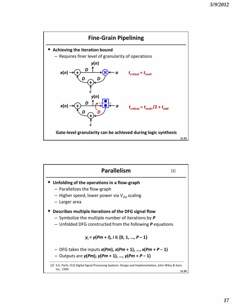
Fine-Grain Pipelining

Achieving the iteration bound

– Requires finer level of granularity of operations

Gate-level granularity can be achieved during logic synthesis

tcritical = tmult

tcritical = tmult /2 + tadd

x(n)

D

a

y(n)

D

D

c

× +

+

x(n)

D

a

y(n)

D

D

c

+

+

11.33

Parallelism

Unfolding of the operations in a flow-graph

– Parallelizes the flow-graph

– Higher speed, lower power via VDD scaling

– Larger area

Describes multiple iterations of the DFG signal flow

– Symbolize the multiple number of iterations by P

– Unfolded DFG constructed from the following P equations

– DFG takes the inputs x(Pm), x(Pm + 1), …, x(Pm + P − 1)

– Outputs are y(Pm), y(Pm + 1), …, y(Pm + P − 1)

yi = y(Pm + i), i ∈ {0, 1, …, P – 1}

[2] K.K. Parhi, VLSI Digital Signal Processing Systems: Design and Implementation, John Wiley & Sons Inc., 1999.

[2]

11.34

5/9/2012

18

Unfolding

To construct P unfolded DFG

– Draw P copies of all the nodes in the original DFG

– The P input nodes take in values x(Pm), …, x(Pm + P − 1)

– Connect the nodes based on precedence constraints of DFG

– Each delay in unfolded DFG is P-slow

– Tap outputs x(Pm), …, x(Pm + P − 1) from the P output nodes

x(n)

y(n)

D

a y(2m)

y(2m + 1)

D* = 2D

Original Unfolded with P = 2

u u1 v

u2

v1

v2 a

a x(2m)

x(2m + 1) y(2m) = a∙y(2m − 1) + x(2m) y(2m + 1) = a∙y(2m) + x(2m + 1)

11.35

Unfolding for Constant Throughput

Unfolding recursive flow-graphs

– Maximum attainable throughput limited by iteration bound

– Unfolding does not help if iteration bound already achieved

x(n) a

y(n)

D × +

y(2m)

y(2m + 1)

D* = 2D

a

a x(2m)

x(2m + 1)

+

+

×

×

y(n) = x(n) + a∙y(n − 1)

y(2m) = x(2m) + a∙y(2m − 1)

y(2m + 1) = x(2m + 1) + a∙y(2m)

tcritical = tadd + tmult

tcritical = 2∙tadd + 2∙tmult

tcritical/iter = tcritical /2

Throughput remains the same

11.36

5/9/2012

19

Unfolding FIR Systems for Higher Throughput

Throughput can be increased with effective pipelining

y(n)

x(n)

d c b a

+ + + D D D

y(2m − 1)

x(2m + 1)

d c b a

+ + + D

y(2m − 2)

d c b a

+ + + D D

x(2m)

y(n) = a∙x(n) + b∙x(n − 1) + c∙x(n − 2) + d∙x(n − 3)

y(2m − 2) = a∙x(2m − 2) + b∙x(2m − 3) + c∙x(2m − 4) + d∙x(2m − 5)

y(2m − 1) = a∙x(2m − 1) + b∙x(2m − 1) + c∙x(2m − 3) + d∙x(2m − 4)

tcritical = tadd + tmult

tcritical = tadd + tmult

tcritical/iter = tcritical /2

Throughput doubles!!

D

D

*

* Register retiming moves

11.37

Introduction to Scheduling

Dictionary definition

– The coordination of multiple related tasks into a time sequence

– To solve the problem of satisfying time and resource constraints between a number of tasks

Data-flow-graph scheduling

– Data-flow-graph iteration ● Execute all operations in a sequence

● Sequence defined by the signal flow in the graph

– One iteration has a finite time of execution Titer

– Constraints on Titer given by throughput requirement

– If required Titer is long

● Titer can be split into several smaller clock cycles ● Operations can be executed in these cycles

● Operations executing in different cycles can share hardware

11.38

5/9/2012

20

Area-Throughput Tradeoff

Scheduling provides a means to tradeoff throughput for area

– If Titer = Tclk all operations required dedicated hardware units

– If Titer = N∙Tclk , N > 1, operations can share hardware units

x1(n) x2(n)

y(n)

v1 v2

v3

v4

Titer = Tclk

Tclk

No hw sharing

3 multipliers and 1 adder 2 multipliers and 1 adder

×

+

×

×

x1(n) x2(n)

y(n)

v1 v2

v3

v4

Titer Shared

hardware

×

+

×

×

11.39

Schedule Assignment

Available: hardware units H and N clock cycles for execution

– For each operation, schedule table records ● Assignment of hardware unit for execution, H(vi)

● Assignment of time of execution, p(vi)

Tclk

x1(n) x2(n)

y(n)

v1 v2

v3

v4

Titer Shared

hardware

×

+

×

×

Schedule Add 1 Mult 1 Mult 2

Cycle 1 x v1 v2

Cycle 2 v3 x x

Cycle 3 x x v4

Schedule Table

H(v1) = Multiplier 1 H(v2) = Multiplier 2 H(v3) = Adder 1 H(v4) = Multiplier 1

p(v1) = 1 p(v2) = 1 p(v3) = 2 p(v4) = 3

11.40

5/9/2012

21

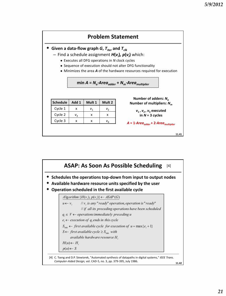
Problem Statement

Given a data-flow graph G, Titer and Tclk

– Find a schedule assignment H(vi), p(vi) which: ● Executes all DFG operations in N clock cycles

● Sequence of execution should not alter DFG functionality

● Minimizes the area A of the hardware resources required for execution

Number of adders: Na

Number of multipliers: Nm

A = 1∙Areaadder + 2∙Areamultiplier

v1 , v2 , v3 executed in N = 3 cycles

Schedule Add 1 Mult 1 Mult 2

Cycle 1 x v1 v2

Cycle 2 v3 x x

Cycle 3 x x v4

min A = Na∙Areaadder + Nm∙Areamultiplier

11.41

ASAP: As Soon As Possible Scheduling

Schedules the operations top-down from input to output nodes

Available hardware resource units specified by the user

Operation scheduled in the first available cycle

A lgorithm {H(v i), p(v i)} ASAP (G)

u v i // v i is any "ready" operation, operation is "ready"

// if all its preceding operations have been scheduled

qi V operations immediately preceding u

ei execution of qi ends in this cycle

Smin first available cycle for execution of u max{ei 1}

S first available cycle Smin with

available hardware resource Hi

H(u) Hi

p(u) S

[4] C. Tseng and D.P. Siewiorek, "Automated synthesis of datapaths in digital systems," IEEE Trans. Computer-Aided Design, vol. CAD-5, no. 3, pp. 379-395, July 1986.

[4]

11.42

5/9/2012

22

ASAP Example

Assumptions:

– Titer = 4∙Tclk , N = 4

– Multiplier pipeline: 1

– Adder pipeline: 1

– Available hardware ● 1 multiplier M1

● 1 adder A1

x1(n) x2(n)

y(n)

v1 v2

v3

v4

×

+

×

×

Graph G

Sched. u q e Smin S p(u) H(u)

Step 1 v1 null 0 1 1 1 M1

Step 2 v2 null 0 1 2 2 M1

Step 3 v3 v1 , v2 1 3 3 3 A1

Step 4 v4 v3 2 4 4 4 M1

ASAP scheduling steps

11.43

ASAP Example

x1(n) x2(n)

y(n)

v1 v2

v3

v4

×

+

×

×

Graph G x1(n) x2(n)

y(n)

v1

v2

v3

v4

Tclk

Titer

Final ASAP schedule

Schedule M1 A1

Cycle 1 v1 x

Cycle 2 v2 x

Cycle 3 x v3

Cycle 4 v4 x

Schedule Table M1

M1

A1

M1

Schedules “ready” operations in the first cycle with available resource

11.44

5/9/2012

23

Scheduling Algorithms

More heuristics

– Heuristics vary in their selection of next operation to scheduled

– This selection strongly determines the quality of the schedule

– ALAP: As Late As Possible scheduling ● Similar to ASAP except operations scheduled from output to input

● Operation “ready” if all its succeeding operations scheduled

– ASAP, ALAP do not give preference to timing-critical operations ● Can result in timing violations for fixed set of resources

● More resource/area required to meet the Titer timing constraint

– List scheduling ● Selects the next operation to be scheduled from a list

● The list orders the operations according to timing criticality

11.45

List Scheduling

Assign precedence height PH(vi) to each operation

– PH(vi) = length of longest combinational path rooted by vi

– Schedule operations in descending order of precedence height

x1(n) x2(n)

y1(n)

v1 v2

v4

×

+

×

y2(n)

+

x3(n)

× v3

v5

v6 × Possible scheduling sequence

ASAP v1→ v2→ v3 → v4→ v5→ v6

LIST v3→ v2→ v5 → v1→ v4→ v6

PH(v1) = T(v4) = 1

PH(v2) = T(v5) + T(v6) = 3

PH(v3) = T(v5) + T(v6) = 3 PH(v5) = T(v6) = 2

PH(v4) = 0, PH(v6) = 0

tadd = 1, tmult = 2

[5] S. Davidson et. al., "Some experiments in local microcode compaction for horizontal machines," IEEE Trans. Computers, vol. C-30, no. 7, pp. 460-477, July 1981.

[5]

11.46

5/9/2012

24

Comparing Scheduling Heuristics: ASAP

x1(n) x2(n)

y1(n)

v1 v2

v4

y2(n)

x3(n)

v5

M1

A1

M2

v3 M1

A1

v6 M1

Timing violation

Titer

ASAP schedule infeasible, more resources required to satisfy timing

Titer = 5∙Tclk , N = 5

Pipeline depth Multiplier: 2 Adder: 1

Available hardware 2 mult: M1, M2

1 add: A1

11.47

Comparing Scheduling Heuristics: LIST

LIST scheduling feasible, with 1 adder and 2 multipliers in 5 time steps

Titer = 5∙Tclk , N = 5

Pipeline depth Multiplier: 2 Adder: 1

Available hardware 2 mult: M1, M2

1 add: A1

x1(n) x2(n)

y1(n)

v1

v2

v4

y2(n)

x3(n)

v5

M1

A1

M2

v3 M1

A1

v6 M1

Titer

11.48

5/9/2012

25

Inter-Iteration Edges: Timing Constraints

Edge e : v1 → v2 with zero delay forces precedence constraints

– Result of operation v1 is input to operation v2 in an iteration

– Execution of v1 must precede the execution of v2

Edge e : v1 → v2 with delays represent relaxed timing constraints

– If R delays present on edge e

– Output of v1 in I th iteration is input to v2 in (I + R)th iteration

– v1 not constrained to execute before v2 in the I th iteration

Delay insertion after scheduling

– Use folding equations to compute the number of delays/registers to be inserted on the edges after scheduling

11.49

Inter-Iteration Edges

x1(n) x2(n)

y1(n)

v1 v2

v4

×

+

×

y2(n)

+

x3(n)

× v3

v5

v6 ×

D

Inter-iteration edge e : v4 → v5

v5 is not constrained to execute after v4 in an iteration

Insert registers on edge e for correct operation

x1(n) x2(n)

y1(n)

v1

v2

v4

y2(n)

x3(n)

v5

M1

A1

M2

v3 M1

A1

v6

M1

Titer

11.50

5/9/2012

26

Folding

Maintain precedence constraints and functionality of DFG

– Route signals to hardware units at the correct time instances

– Insert the correct number of registers on edges after scheduling

v1 mapped to unit H1 v2 mapped to unit H2

2 pipeline stages in H1

1 pipeline stage in H2

v1 v2

w

Original Edge Scheduled Edge

H1 H2

f v11 v12 v2

d(v1) = 2 2 pipeline stages

d(v2) = 1 1 pipeline stage

Compute value of f which maintains precedence

11.51

Folding Equation

Number of registers on edges after folding depends on

– Original number of delays w, pipeline depth of source node

– Relative time difference between execution of v1 and v2

v1 v2

w

H1 H2

f v11 v12 v2

M1

A1

p(v1) = 1

p(v2) = 3

d(v1) = 2

N clock cycles per iteration w delays → N∙w delay in schedule

f = N∙w – d(v1) + p(v2) – p(v1)

Legend d: delay, p: schedule

11.52

5/9/2012

27

Scheduling Example

v1 v2 e1

y(n) x(n) 2D

v1 v2 e1

y(n) x(n) D D

z−1

z−2 v y(n) x(n)

(a) Original edge

(b) Retimed edge

(c) Retimed edge after scheduling

Edge scheduled using folding equations

Folding factor (N) = 2

Pipeline depth

− d(v1) = 2

− d(v2) = 2

Schedule

− p(v1) = 1

− p(v2) = 2

11.53

Efficient Retiming & Scheduling

Retiming with scheduling

– Additional degree of freedom associated with register movement results in less area or higher throughput schedules

Challenge: Retiming with scheduling

– Time complexity increases if retiming done with scheduling

Approach: Low-complexity retiming solution

– Pre-process data flow graph (DFG) prior to scheduling

– Retiming algorithm converges quickly (polynomial time)

– Time-multiplexed DSP designs can achieve faster throughput

– Min-period retiming can result in reduced area as well

Result: Performance improvement

– An order of magnitude reduction in the worst-case time-complexity

– Near-optimal solutions in most cases

11.54

5/9/2012

28

DSP Design

N

Scheduling (current)

Scheduling (ILP) with

BF retiming

Scheduling with pre-processed retiming

Area CPU(s) Area CPU(s) Area CPU(s)

Wave filter

16 NA NA 8 264 14 0.39

17 13 0.20 7 777 8 0.73

Lattice filter

2 NA NA 41 0.26 41 0.20

4 NA NA 23 0.30 23 0.28

8-point DCT

3 NA NA 41 0.26 41 0.21

4 NA NA 28 0.40 28 0.39

NA – scheduling infeasible without retiming

Near-optimal solutions at significantly reduced worst-case runtime

Results: Area and Runtime

11.55

Scheduling Comparison

Scheduling with pre-retiming outperforms scheduling

– Retiming before scheduling enables higher throughput

– Lower power consumption with VDD scaling for same speed

(1.0) (1.0)

(0.9)

(0.84)

LIST + VDD scaling

(0.78)

(0.75)

(0.71)

(1.0) (1.0)

(1.0)

(1.0)

(0.81)

(0.78)

(0.71)

Second-order IIR 16-tap FIR (transposed)

LIST + pre-retiming + VDD scaling

Throughput (MS/s)

80 114 148 182 216 250 0.1

1

0.1

1

100 150 200 250 300 350

Po

wer

Throughput (MS/s)

(no

rmal

ize

d)

(VDD) (VDD)

(0.81) (0.88)

11.56

5/9/2012

29

Summary

DFG automation algorithms

– Retiming, pipelining

– Parallelism

– Scheduling

Simulink-based design optimization flow

– Parameterized architectural transformations

– Resultant optimized architecture available in Simulink

Energy, area, performance tradeoffs with

– Architectural optimizations

– Carry-save arithmetic

– Voltage scaling

11.57

References

C. Leiserson and J. Saxe, "Optimizing Synchronous Circuitry using Retiming," Algorithmica, vol. 2, no. 3, pp. 211–216, 1991.

R. Nanda, DSP Architecture Optimization in Matlab/Simulink Environment, M.S. Thesis, University of California, Los Angeles, 2008.

K.K. Parhi, VLSI Digital Signal Processing Systems: Design and Implementation, John Wiley & Sons Inc., 1999.

C. Tseng and D.P. Siewiorek, "Automated Synthesis of Datapaths in Digital Systems," IEEE Trans. Computer-Aided Design, vol. CAD-5, no. 3, pp. 379–395, July 1986.

S. Davidson et al., "Some Experiments in Local Microcode Compaction for Horizontal Machines," IEEE Trans. Computers, vol. C-30, no. 7, pp. 460–477, July 1981.

11.58

5/9/2012

30

Course Wiki – CAD Tutorials

DSP Architect Tool

Source code

Tested with Matlab 2007b and SynDSP 3.6

11.59