University of Massachusetts Amherst University of Massachusetts Amherst

ScholarWorks@UMass Amherst ScholarWorks@UMass Amherst

Masters Theses 1911 - February 2014

2010

Data Fusion for the Problem of Protein Sidechain Assignment Data Fusion for the Problem of Protein Sidechain Assignment

Yang Lei University of Massachusetts Amherst

Follow this and additional works at: https://scholarworks.umass.edu/theses

Part of the Biochemical and Biomolecular Engineering Commons, and the Signal Processing

Commons

Lei, Yang, "Data Fusion for the Problem of Protein Sidechain Assignment" (2010). Masters Theses 1911 - February 2014. 505. Retrieved from https://scholarworks.umass.edu/theses/505

This thesis is brought to you for free and open access by ScholarWorks@UMass Amherst. It has been accepted for inclusion in Masters Theses 1911 - February 2014 by an authorized administrator of ScholarWorks@UMass Amherst. For more information, please contact scholarworks@library.umass.edu.

DATA FUSION FOR THE PROBLEM OF PROTEINSIDECHAIN ASSIGNMENT

A Thesis Presented

by

YANG LEI

Submitted to the Graduate School of theUniversity of Massachusetts Amherst in partial fulfillment

of the requirements for the degree of

MASTER OF SCIENCE IN ELECTRICAL AND COMPUTER ENGINEERING

September 2010

Electrical and Computer Engineering

DATA FUSION FOR THE PROBLEM OF PROTEINSIDECHAIN ASSIGNMENT

A Thesis Presented

by

YANG LEI

Approved as to style and content by:

Ramgopal R. Mettu, Chair

Paul Siqueira, Member

Dennis L. Goeckel, Member

C. V. Hollot, Department HeadElectrical and Computer Engineering

To my great parents and grandparents...

ACKNOWLEDGMENTS

I am very grateful for my advisor Prof. Ramgopal Mettu’s instructions and help.

He always encourages me and inspires me with lots of valuable insights in our meet-

ings. He is an easy-going professor and also a very helpful friend to me. After I

get fascinated by the area of Microwave Remote Sensing, he generously supports my

thoughts and approves me to select whatever courses I like. We also aim to make

the types of the techniques described in the thesis applicable in both bioinformatics

and remote sensing. There is an old Chinese phrase saying “He who teaches me for

one day is my father for life”. I will always remember Prof. Mettu’s help and this

fantastic two-year master study. I would like to thank Prof. Paul Siqueira and Prof.

Dennis Goeckel very much for their constructive suggestions and the favor of being my

committee members. Finally, I want to give my genuine thanks to my great parents

and grandparents without whom I cannot be who I am now.

iv

ABSTRACT

DATA FUSION FOR THE PROBLEM OF PROTEINSIDECHAIN ASSIGNMENT

SEPTEMBER 2010

YANG LEI

M.S., UNIVERSITY OF MASSACHUSETTS AMHERST

Directed by: Professor Ramgopal R. Mettu

In this thesis, we study the problem of protein side chain assignment (SCA) given

multiple sources of experimental and modeling data. In particular, the mechanism

of X-ray crystallography (X-ray) is re-examined using Fourier analysis, and a novel

probabilistic model of X-ray is proposed for SCA’s decision making. The relationship

between the measurements in X-ray and the desired structure is reformulated in terms

of Discrete Fourier Transform (DFT). The decision making is performed by devel-

oping a new resolution-dependent electron density map (EDM) model and applying

Maximum Likelihood (ML) estimation, which simply reduces to the Least Squares

(LS) solution. Calculation of the confidence probability associated with this decision

making is also given. One possible extension of this novel model is the real-space

refinement when the continuous conformational space is used.

Furthermore, we present a data fusion scheme combining multi-sources of data

to solve SCA problem. The merit of our framework is the capability of exploiting

multi-sources of information to make decisions in a probabilistic perspective based on

Bayesian inference. Although our approach aims at SCA problem, it can be easily

transplanted to solving for the entire protein structure.

v

TABLE OF CONTENTS

Page

ACKNOWLEDGMENTS . . . . . . . . . . . . . . . . . . . . . . . . . . . . . . . . . . . . . . . . . . . . . iv

ABSTRACT . . . . . . . . . . . . . . . . . . . . . . . . . . . . . . . . . . . . . . . . . . . . . . . . . . . . . . . . . . v

LIST OF TABLES . . . . . . . . . . . . . . . . . . . . . . . . . . . . . . . . . . . . . . . . . . . . . . . . . . .viii

LIST OF FIGURES . . . . . . . . . . . . . . . . . . . . . . . . . . . . . . . . . . . . . . . . . . . . . . . . . . . ix

CHAPTER

1. INTRODUCTION . . . . . . . . . . . . . . . . . . . . . . . . . . . . . . . . . . . . . . . . . . . . . . . . . 1

1.1 Protein Structure . . . . . . . . . . . . . . . . . . . . . . . . . . . . . . . . . . . . . . . . . . . . . . . . . 3

1.1.1 Amino Acid and Backbone . . . . . . . . . . . . . . . . . . . . . . . . . . . . . . . . . . 31.1.2 Dihedral Angles . . . . . . . . . . . . . . . . . . . . . . . . . . . . . . . . . . . . . . . . . . . . 41.1.3 Side Chain and Rotamers . . . . . . . . . . . . . . . . . . . . . . . . . . . . . . . . . . . 4

1.2 Definition of Electron Density Map . . . . . . . . . . . . . . . . . . . . . . . . . . . . . . . . . 51.3 Definition of Protein SCA Problem . . . . . . . . . . . . . . . . . . . . . . . . . . . . . . . . . 61.4 Related Work . . . . . . . . . . . . . . . . . . . . . . . . . . . . . . . . . . . . . . . . . . . . . . . . . . . . 8

1.4.1 Real-space Refinement . . . . . . . . . . . . . . . . . . . . . . . . . . . . . . . . . . . . . . 81.4.2 Discrete Fourier Summation in Reciprocal-space Refinement . . . . . 91.4.3 General Data Fusion Techniques . . . . . . . . . . . . . . . . . . . . . . . . . . . . 101.4.4 Data Fusion in Protein Structure Refinement . . . . . . . . . . . . . . . . . 101.4.5 Protein Model-building Softwares using Real-space

Refinement . . . . . . . . . . . . . . . . . . . . . . . . . . . . . . . . . . . . . . . . . . . . 11

1.5 Outline . . . . . . . . . . . . . . . . . . . . . . . . . . . . . . . . . . . . . . . . . . . . . . . . . . . . . . . . 12

2. X-RAY DATA COLLECTION ANDRESOLUTION-DEPENDENT ELECTRON DENSITYMODEL . . . . . . . . . . . . . . . . . . . . . . . . . . . . . . . . . . . . . . . . . . . . . . . . . . . . . . . 13

vi

2.1 X-ray Diffraction and Structure Factor . . . . . . . . . . . . . . . . . . . . . . . . . . . . . 132.2 Electron Cloud and Electron Density Map . . . . . . . . . . . . . . . . . . . . . . . . . . 162.3 Resolution-dependent Electron Density Model . . . . . . . . . . . . . . . . . . . . . . . 17

3. ERROR DISTRIBUTION OF RESOLUTION-DEPENDENTELECTRON DENSITIES . . . . . . . . . . . . . . . . . . . . . . . . . . . . . . . . . . . . . . 25

3.1 Discrete Fourier Transform (DFT) Representation . . . . . . . . . . . . . . . . . . . 263.2 The Probability Distribution of Electron Densities . . . . . . . . . . . . . . . . . . . 333.3 Statistical Properties . . . . . . . . . . . . . . . . . . . . . . . . . . . . . . . . . . . . . . . . . . . . . 42

3.3.1 Maximum Likelihood (ML) estimate of protein structures . . . . . . . 423.3.2 Discrete-case Parseval’s Theorem . . . . . . . . . . . . . . . . . . . . . . . . . . . . 43

3.4 Decision Making and Confidence Probability . . . . . . . . . . . . . . . . . . . . . . . . 44

3.4.1 Decision Rules for Refinement . . . . . . . . . . . . . . . . . . . . . . . . . . . . . . 453.4.2 Confidence Probability Calculation . . . . . . . . . . . . . . . . . . . . . . . . . . 46

4. EXPERIMENTAL RESULTS USING X-RAY DATA ONLY . . . . . . 49

5. DATA FUSION FOR PROTEIN SIDE CHAINASSIGNMENT . . . . . . . . . . . . . . . . . . . . . . . . . . . . . . . . . . . . . . . . . . . . . . . . 54

5.1 Validation of Multiple Sources of Information. . . . . . . . . . . . . . . . . . . . . . . . 54

5.1.1 Nuclear Magnetic Resonance (NMR) . . . . . . . . . . . . . . . . . . . . . . . . . 545.1.2 Potential Energy Calculation . . . . . . . . . . . . . . . . . . . . . . . . . . . . . . . 55

5.2 Data Fusion Schemes . . . . . . . . . . . . . . . . . . . . . . . . . . . . . . . . . . . . . . . . . . . . . 59

5.2.1 Weighted Bayesian Data Fusion . . . . . . . . . . . . . . . . . . . . . . . . . . . . . 605.2.2 Results of Data Fusion for a Simplified SCA Problem . . . . . . . . . . 64

6. CONCLUSIONS AND FUTURE WORK . . . . . . . . . . . . . . . . . . . . . . . . . 68

BIBLIOGRAPHY . . . . . . . . . . . . . . . . . . . . . . . . . . . . . . . . . . . . . . . . . . . . . . . . . . . 70

vii

LIST OF TABLES

Table Page

4.1 Resolution, secondary structures and accuracy of the testedproteins . . . . . . . . . . . . . . . . . . . . . . . . . . . . . . . . . . . . . . . . . . . . . . . . . . . . . 50

viii

LIST OF FIGURES

Figure Page

1.1 Amino Acid and Protein Structure. The chemical compositionof an amino acid [36]. The primary, secondary and tertiarystructure of a protein [3]. . . . . . . . . . . . . . . . . . . . . . . . . . . . . . . . . . . . . . . . 3

1.2 Dihedral Angles [21]. . . . . . . . . . . . . . . . . . . . . . . . . . . . . . . . . . . . . . . . . . . . . . . 4

1.3 Rotamers [42]. . . . . . . . . . . . . . . . . . . . . . . . . . . . . . . . . . . . . . . . . . . . . . . . . . . . 5

1.4 Carbon Atomic Electron Cloud [25]. . . . . . . . . . . . . . . . . . . . . . . . . . . . . . . . . . 6

2.1 X-ray Crystallography Experiment [18]. . . . . . . . . . . . . . . . . . . . . . . . . . . . . . 14

2.2 Ewald Sphere and Reciprocal Space [33]. . . . . . . . . . . . . . . . . . . . . . . . . . . . . 15

2.3 Spherical Gaussian Electron Cloud [14]. . . . . . . . . . . . . . . . . . . . . . . . . . . . . 17

2.4 3D Impulse Response Formed by Sinc Function . . . . . . . . . . . . . . . . . . . . . . 21

2.5 8-division method vs. direct numerical integral in the 1D simulationof resolution-dependent EDM for a carbon atom at 1A . . . . . . . . . . . . 23

2.6 8-division method vs. direct numerical integral in the 1D simulationof resolution-dependent EDM for a carbon atom at 2.5A . . . . . . . . . . . 23

2.7 8-division method vs. direct numerical integral in the 1D simulationof resolution-dependent EDM for a carbon atom at 4A . . . . . . . . . . . . 24

3.1 Comparisons of 3D DFT results between spherical and cubic filters . . . . . 38

3.2 1D simulation of EDM measurements . . . . . . . . . . . . . . . . . . . . . . . . . . . . . . 41

4.1 Accuracy of the Prediction at Different Resolutions . . . . . . . . . . . . . . . . . . 50

4.2 The clash occurred in high-quality EDM between LYS and itsneighbor residue . . . . . . . . . . . . . . . . . . . . . . . . . . . . . . . . . . . . . . . . . . . . . . 51

ix

4.3 Accuracy vs. Confidence Probability at Different Resolutions . . . . . . . . . . 53

5.1 Data Script of Ubiquitin NMR Restraint Grid . . . . . . . . . . . . . . . . . . . . . . . 55

5.2 The Best Rotamer vs. the Best-fit Rotamer of GLU with the distancebetween GLU’s Cγ and the nearby ARG’s Cγ . . . . . . . . . . . . . . . . . . . . 56

5.3 The top three best-fit rotamers of LYS residue (id: 82) in pdb file“2zr4” . . . . . . . . . . . . . . . . . . . . . . . . . . . . . . . . . . . . . . . . . . . . . . . . . . . . . . 58

5.4 The fourth best-fit (also the best) rotamer of LYS residue (id: 82) inpdb file “2zr4” . . . . . . . . . . . . . . . . . . . . . . . . . . . . . . . . . . . . . . . . . . . . . . . 59

5.5 Data Fusion Schemes . . . . . . . . . . . . . . . . . . . . . . . . . . . . . . . . . . . . . . . . . . . . . 60

5.6 Data fusion vs. X-ray data only for the prediction of LYS residues atdifferent resolutions . . . . . . . . . . . . . . . . . . . . . . . . . . . . . . . . . . . . . . . . . . . 67

x

CHAPTER 1

INTRODUCTION

It is known that studying protein 3D structures is of great importance to un-

derstand the biological processes at a molecular level. Since there is a close rela-

tionship between protein structures and functionalities, we can exploit 3D structures

for biomedical purposes, e.g. developing new drugs. There are currently more than

60,000 protein structures deposited in Protein Data Bank (PDB). As the experimen-

tal methods become more high-throughput, researchers are seeking efficient compu-

tational methods to assist in interpreting data for protein structure determination.

Currently, the most effective experimental method for 3D structure determination is

X-ray crystallography, although other techniques complement it providing additional

useful information.

A typical protein 3D structure is comprised of a backbone (i.e. main chain) and

side chains, where the backbone mainly describes the protein folding characteristics

and side chains are detailed structure. At a high level, for a protein under test,

we usually get the primary sequence according to the transcription and translation

from DNA segments, and utilize experimental data to resolve potential variations of

the backbone and the side chains respectively. In most existing softwares (e.g. O,

XtalView), there are several standard criteria to obtain the backbone carbon atom

positions [31]. By searching a database of refined backbone fragments, the main chain

can finally be resolved with high accuracy.

The determination of side chain conformations, also known as side chain assign-

ment (SCA), is a different and challenging problem since the measurements of side

1

chains are usually much poorer than those for the main chain. In this thesis, we only

focus on the SCA problem; however, solving the entire protein structure is our ulti-

mate goal, and we expect that our method can be extended to also handle backbone

tracing. Current state-of-the-art methods attacking the SCA problem can be divided

into two categories. The first class of methods predict side chain conformations with

the principle of global minimum energy, since it is always assumed the native protein

structure is a stable and dynamic equilibrium among all the possible conformations,

hence minimizing the total potential energy. However, results for this type of methods

are not accurate due to our limited understanding of the protein folding mechanism

and the expression of the protein potential energy. The second class of methods seek

to determine protein structures experimentally. In fact, each of the deposited pro-

tein structures in PDB was either solved by X-ray crystallography (X-ray) or Nuclear

Magnetic Resonance (NMR). The data interpretation of both X-ray and NMR has

already been studied with a wealth of valuable results brought forward. For X-ray,

the process of data interpretation is usually carried out in reciprocal- and real-space

refinements. This is especially in reciprocal space, since there is a shortage of effective

models for real space. However, the improved experimental techniques, e.g. Multi-

wavelength Anomalous Diffraction (MAD), have recently renewed the general interest

in real-space refinement, which is more suited to fitting partial model to X-ray data.

In this thesis, we derive a novel framework of real-space refinement based on Fourier

analysis.

Researchers have also attempted to combine the experimental methods with stere-

ochemical restraints (i.e. derived from the potential energy) to overcome overfitting

the structural model to the data. The potential energy calculations, also known as

stereochemical restraints, through sophisticated techniques, manage to explain many

types of molecular force fields and thus eliminate the undesirable conformations. It

is also noticed that each data source has some limitations regarding predicting the

2

protein structure accurately. Trials are made to combine different sources of data

but few systematic ways are brought forward. The type of this hybrid model is com-

monly referred to as Data Fusion. Here we apply a fusion scheme for protein side

chain assignment (SCA) problem using Bayesian estimation theory.

1.1 Protein Structure

Since there is a close relationship between functionality and structure, in this

section, we introduce the geometric conventions for representing protein structure.

1.1.1 Amino Acid and Backbone

A protein is a compound that consists of chains of amino acids (See Fig. 1.1(a));

there are twenty types of common amino acids. Each type of amino acid shares a

carbon atom (denoted by Cα), which is attached to an amine group and a carboxylic

acid group. Types of amino acids differ in the side chain (denoted as R in Fig. 1.1(a)).

Multiple amino acids undergo the condensation reaction eliminating water molecules,

and forming a sequence of amino acid residues and peptides.

(a) Amino Acid

(b) Protein Structure

Figure 1.1. Amino Acid and Protein Structure. The chemical composition ofan amino acid [36]. The primary, secondary and tertiary structure of a protein [3].

3

As a result, the polypeptide chain in (Fig. 1.1(b)) is called the protein primary

structure. To differentiate from side chains, we refer to the sequence comprised of

Cα atoms and peptides as the backbone. Furthermore, we refer to the α-helix and

β-sheet as the secondary structure, and the three dimensional coordinates of all the

atoms as the tertiary structure.

1.1.2 Dihedral Angles

Since the peptide forms a stable plane structure, which is much more rigid than

any other bonds, the freedom of the protein folding is mostly based on the torsion

angles in the backbone and the side chain. This is illustrated in Fig. 1.2. As shown,

dihedral angles φ and ψ denote the torsion angles of the backbone peptide, and χ1, χ2,

χ3, χ4 are the dihedral angles within the side chain. Note the χ angles are assigned

hierarchically meaning some side chains may not have all the four χ angles.

1.1.3 Side Chain and Rotamers

Figure 1.2. Dihedral Angles [21].

In Section 1.1.2, we noted that the side chain

conformations can be represented by the possible

combinations of the χ angles. Since there are four

dihedral-angle degrees of freedom, there can be

infinitely many combinations of (χ1, χ2, χ3, χ4).

Each combination of the side chain dihedral an-

gles define a unique side chain conformation, usu-

ally denominated as a rotational isomer or ro-

tamer [12] as shown in Fig. 1.3. Technically, re-

searchers find out that only a finite subset of ro-

tamers are observed for each residue type [12].

4

Figure 1.3. Rotamers [42].

Also, it is known that not all the rotamers oc-

cur with equal frequency (e.g. there is some fre-

quency distribution over the rotamers of each par-

ticular residue type). The most widely used ro-

tamer libraries [11][24] are thus constructed stor-

ing the frequency information of each rotamer for

certain residue type. These rotamer libraries fall into two categories, backbone-

dependent libraries and backbone-independent ones. They only differ in whether

to use the information of the φ and ψ backbone dihedral angles. Obviously, the

backbone-dependent rotamer libraries are more useful and informative. In the work

described here, the Dunbrak Backbone-Dependent Rotamer Library [11] was chosen.

1.2 Definition of Electron Density Map

To interpret and model X-ray data, also known as Electron Density Map (EDM),

we need to describe the electron cloud. The most accurate description of electron

cloud is given by quantum mechanics; however, due to the complexity of calculation,

we prefer the classical view of electron density model. Above all, it is necessary to

have an overview about the form of the electron cloud.

It was reported in September 2009 that, physicists photographed the carbon elec-

tron cloud Fig. 1.4 for the very first time.

In quantum mechanics, an electron does not exist as a single point, but spreads

around a nuclei as cloud referred to as orbital. In Fig. 1.4, there are two arrangements

of electron cloud for a carbon atom. As an extension of this, other atoms, such as

oxygen, nitrogen and sulfur, have their own corresponding electron clouds as well.

The intensity of a bright blue point in Fig. 1.4 represents the sum of the probabilities

that each of the electrons is present at this current point, which can be computed by

the well-known Schrodinger equation with lots of effort. The calculation is computa-

5

Figure 1.4. Carbon Atomic Electron Cloud [25].

tionally intractable when the electron clouds pertaining to a covalent bond should be

addressed, which is rather common in protein structures. For the above mentioned

reasons, we need to develop a simplified electron cloud model, which will be discussed

in Section 2.2. In this section, we give a definition of electron number density and

electron (number) density map.

Definition 1 (Electron Number Density and Electron Density Map). Electron num-

ber density ρ(~r) at a point ~r = (x, y, z), by meaning, is the number of electrons

enclosed by a closed surface as the volume approaches zero. When the position vec-

tor ~r goes over a single unit cell of the crystal, the three dimensional electron density

function ρ(~r) is the widely-used Electron Density Map (EDM).

Definition 1 is equivalent to the above mentioned probability-based definition in

quantum mechanics. Moreover, this is the ideal case meaning no resolution limitation

is involved. As we will see later (Section 2.3), the effect of resolution makes the

practical electron density value deviate from the ideal value ρ(~r), and the EDM is

thus blurred. Generally, the higher the resolution is, the closer the electron density

value is to ρ(~r), and thus the higher quality of EDM.

1.3 Definition of Protein SCA Problem

Now we define our problem of side chain assignment as follows.

6

Definition 2 (Side Chain Assignment). The side chain conformation at a particular

residue i (1 ≤ i ≤ N) is determined by selecting the most likely rotamer from the

rotamer set Θi given that residue’s backbone atoms and φ, ψ dihedral angles if using

the backbone-dependent library. The criterion of selection in terms of likelihood could

be the EDM fit, NMR restraints and stereochemical restraints, etc.

If a protein has N residues as a whole, the set of the side chain conformational

space is a Cartesian product Θ1 × Θ2 × · · · × ΘN , denoted by Θ. Let S represent a

candidate side chain conformation for all N residues of the current protein, and we

can rewrite the above mentioned problem in a mathematical way.

S∗ = arg maxS∈Θ

P (S | EDM,NMR)

= arg maxS∈Θ

f(EDM,NMR | S) P (S) (1.1)

Given the structure, different sources of experimental data are assumed to be

class-conditionally independent [38].

S∗ = arg maxS∈Θ

f(EDM,NMR | S) P (S)

= arg maxS∈Θ

f(EDM | S) f(NMR | S) P (S) (1.2)

In (1.2), P (EDM | S) comes from the likelihood of X-ray data. Given the struc-

ture, the electron densities of different voxels in the crystal can be made independent

(see Chapter 3). In other words, P (EDM | S) can be broken down to individual

terms P (LEDM | Si) associated with local electron density map (LEDM), where Si

represents the side chain conformation of the ith residue. Similarly, P (NMR | S)

can be expanded to pairwise terms in the form of P (LNMR | Si and Sj) after the

decorrelation of NMR data. As for the priors P (S), we can use Boltzmann relation-

ship [16][41] accounting for the contribution of the potential energy function, which

is comprised with self- and pairwise- energy terms.

7

1.4 Related Work

1.4.1 Real-space Refinement

The idea of real-space refinement is first introduced by Diamond [8], where a Gaus-

sian electron cloud model is demonstrated. Although this refinement is successful for

several proteins with high-quality EDM’s, the modeled EDM does not take the reso-

lution limitation into account. Also, since before multiple isomorphous replacement

and multi-wavelength anomalous dispersion are used to give phase measurements,

only amplitudes of structure factors can be measured, it is necessary to estimate

the phase information using molecular replacement [31]. The EDM’s constructed

utilizing this inaccurate phase information are definitely not reliable for real-space

fitting. However, only amplitudes of structure factors are needed for reciprocal-space

refinement, which surpasses real-space refinement from then on. For the definitions

of reciprocal- and real-space refinements, we draw an analogy between X-ray crystal-

lography and Signal Processing (SP). Since structure factors and electron densities

are continuous Fourier series pair, we can consider real space as time domain in SP,

and reciprocal space as frequency domain. Through reciprocal-space refinement, only

the amplitude information of measured structure factors is refined; however, as for

real-space refinement, the electron densities, or equivalently the complex structure

factors, are improved, since they are a continuous Fourier series pair.

Maximum Likelihood (ML) is a well-known technique for fitting the model to

measurements using statistical fundamentals. To perform ML estimation, we have to

find both the modeled data (i.e. forward model) and the fitting criterion (i.e. error

model). Specifically, for real-space refinement, the modeled data refers to a resolution-

dependent EDM model, and the fitting criterion is the probability distribution of each

sampled electron density in the observed EDM, given the modeled EDM. The model

of resolution-dependent EDM is given by Chapman [4], which is valid for the situation

that the measurements in X-ray are truncated by a limiting sphere. For the fitting

8

criterion, we need to compare the modeled EDM with the EDM constructed from

measurements in some reasonable way. It is necessary to mention that we could

make local comparisons in real-space refinement, which does not hold for reciprocal

space. The local EDM comparison can be used in reciprocal-space refinement [20] as

a matching score, but the real application in real-space refinement is by Zou et al.

[45]. The simple Gaussian model in [8] is used and two types of fitting measures are

proposed (i.e. convolution product and absolute difference). Both measures are taken

over the voxel of a amino acid in the EDM, or local EDM. However, neither of these

is based on the probability distribution of the electron densities in the local EDM. We

will show the error distribution of electron densities at each sampled 3D grid point in

the entire EDM, which has not been looked into before. To our knowledge, the only

description of real-space fitting error is the mean square error (MSE) of the entire

EDM, which is derived from Parseval’s Theorem [31], but not for individual sampled

points.

1.4.2 Discrete Fourier Summation in Reciprocal-space Refinement

Although electron density values and structure factors are conventionally related

by Continuous Fourier Series (CFS), it is desirable to connect them through Discrete

Fourier Summation (DFS), which is also called Discrete Fourier Transform (DFT).

Both reciprocal- and real-space refinements utilize the relationship between structure

factors and electron densities, so the DFT representation can be used for both cases.

As seen later, we can use the DFT representation for real-space refinement to achieve

the probability distribution of sampled electron densities, i.e. the error model.

The DFT representations for both reciprocal- and real-space refinements turn

out to be the same, but the problems of aliasing are different, since there is no

truncation of structure factors (e.g. limiting sphere) in reciprocal-space refinement.

So for reciprocal-space refinement, the error from aliasing can only be reduced but not

9

eliminated; while for real-space refinement, we can absolutely overcome the aliasing

by selecting the sampling frequency appropriately.

In reciprocal-space refinement, structure factors are usually calculated by perform-

ing the DFT since it can be implemented efficiently using the Fast Fourier Transform

(FFT). Sayre [35] first showed that the calculation of structure factors can be done

using DFS, despite the fact that FFT had not been developed yet; he also discussed

the problem of aliasing. Ten Eyck [39] and Navaza [28] extend Sayre’s work and

address the aliasing problem.

1.4.3 General Data Fusion Techniques

In classification problem using remote sensing data, Swain represents the condi-

tional probability of each class given multi-source data by assuming different types

of data are independent, and assigning the reliability weights to individual marginal

probabilities [38][1]. A final decision can be made by maximizing this weighted joint

likelihood. This process is usually called pre-detection fusion. Bennedikson and Swain

[1] also show that this statistical fusion scheme is equivalent to a neural network ap-

proach. However, sometimes it is difficult to transmit the information of conditional

probability due to channel limitations, researchers intend to make decisions at each lo-

cal data source/sensor quantizing the observations to discrete decisions. Based on the

individual local decisions, we end up with a final decision at the fusion center. Chen

et al. [5] talked about the binary and M-ary decision fusion by performing Bayesian

sampling of the posterior probability. Both schemes are carefully introduced in [19].

As for the current SCA problem, there is no issue of channel limitation involved, thus

we propose to use pre-detection fusion based on Bayesian inference.

1.4.4 Data Fusion in Protein Structure Refinement

Our goal is to combine different sources of experimental data to firstly solve the

SCA problem and then to determine the entire structure. The simplest fusion scheme

10

is a linear combination of sources of data, which can be X-ray and potential energy

[2]. For X-ray, either reciprocal-space [37][15] or real-space [4] matching score is used

as a pseudo-energy term along with the potential energy terms, i.e. stereochemical

restraints. In these works, the linear coefficients are typically adjusted by trial and

error. We will show in Chapter 5 that, our proposed fusion scheme is equivalent

to this linear representation by taking the logarithm and converting probability to

energy; however, our choice of parameters is on a probabilistic basis using Bayesian

inference.

1.4.5 Protein Model-building Softwares using Real-space Refinement

Although most of the existing softwares for protein model-building are associated

with reciprocal-space refinement, there are indeed some packages that successfully

use real-space refinement.

Coot [13] uses the atomic number weighted sum of electron density values around

atomic centers as an X-ray matching score, and the stereochemical restraints as a

potential energy score. ARP/wARP [26] [27] merges model-building and structure

refinement as a single iterative process. Specifically, a hybrid model (comprised of

free-atoms and modeled atoms) and reciprocal-space refinement for building the main

chain (i.e. backbone) go back and forth to improve the solution. For the side chains,

ARP/wARP represents the density as a function of torsion angles and then perform

a real-space torsion angle refinement. The idea of torsion angle refinement dates back

to 1971, when Diamond [8] first introduced real-space refinement. The advantage of

torsion-angle refinement, compared to all-atom Cartesian coordinates refinement, is

the reduction of the dimension of the conformation space, or equivalently increas-

ing the observation to parameter ratio. Examination of stereochemical restraints

follows each iteration. Both RESOLVE [40] and TEXTAL [17] construct databases

respectively comprised with accurately resolved structures and their EDM’s or atomic

11

thermal factors. They only have X-ray matching scores, which is by comparison, be-

tween the local EDM of the unknown structure and the local EDM of some set of

structure templates. As for the local EDM of the template, they either search the

corresponding EDM’s deposited in the database, or build a local EDM, using the

atomic thermal factors stored along with the structure files. In other words, for the

modeled data, neither actually calculates the local EDM from a universal model;

their performances completely rely on the statistics of the database. ACMI [9] also

constructs a database of structure fragments/templates but the local modeled EDM

is computed for the chosen template using some techniques described vaguely in [7].

However, the idea of accounting for the resolution limitation in the modeled EDM is

the same as Chapman’s work [4]. ACMI also includes the stereochemical restraints

as global constraints to eliminate undesirable conformations.

1.5 Outline

In Chapter 2, we explain basic background knowledge about X-ray data collection,

and introduce a novel resolution-dependent EDM model. In Chapter 3, we derive and

analyze a new probabilistic model for X-ray crystallographic data interpretation. We

will show decision making and confidence probability calculation based on this model.

In Chapter 4, we illustrate and discuss the prediction results along with confidence

probabilities at varying resolutions. At last, Chapter 5 validates other possible data

sources, and presents the data fusion scheme with the improved prediction results.

12

CHAPTER 2

X-RAY DATA COLLECTION ANDRESOLUTION-DEPENDENT ELECTRON DENSITY

MODEL

In Chapter 2, we introduce the background knowledge for X-ray crystallography

based on Fourier analysis. In Section 2.1, we show the diffraction principle, the recip-

rocal space for describing the diffraction pattern, and the Fourier relationship between

the electron density function and structure factors. In Section 2.2, a simple Gaussian-

distributed atomic electron density model is presented. The EDM constructed from

this model is called the ideal-case EDM model. By considering the effect of the res-

olution limitation as a filter, Section 2.3 gives a resolution-dependent EDM model,

which is by meaning, a function of resolution.

2.1 X-ray Diffraction and Structure Factor

The diagram of an X-ray crystallography experiment is shown in Fig. 2.1. First,

crystallographers grow a protein crystal, the conditions of which are under strict

control. Then, the crystal is mounted appropriately, allowing rotation around the

center. When the crystal is exposed to an intense X-ray beam, the diffraction pattern

on a sensor screen as the crystal is rotated, is recorded.

When the incident wavefronts impinge on the crystal planes, since electrons of

atoms are secondary radiating sources, and also the wavelength of X-ray (1-100 A) and

the spacing d between unit cells are similar in size, the superposition of scattered waves

will produce a diffraction pattern. The superposed wave propagates constructively

13

Figure 2.1. X-ray Crystallography Experiment [18].

in some directions, and destructively in others. The direction of the constructive

interference is given by Bragg’s equation described by

2d sin θ = nλ. (2.1)

Note that the normal vector to the reflection plane bisects the angle between

incident and reflected waves. As long as a set of planes are spaced equal distance apart,

satisfying (2.1), we refer to these planes as imaginary reflection planes. One treatment

is to increase the incident angle, θ, so that the spacing between the adjoining reflection

planes can be reduced, resulting in the resolution of finer details. This is the basic idea

of rotating the crystal to achieve more reflection information, which will be discussed

later.

To better represent the reflections on the crystal planes, physicists use indices

(h, k, l) with (~a,~b,~c) being the real-space basis vectors. These vectors are the edge

vectors of a single unit cell in the crystal. For the reason stated below, we consider

(h, k, l) as three-dimensional coordinates with respect to the reciprocal-space basis

vectors (~a∗,~b∗,~c∗). The relationship between (~a,~b,~c) and (~a∗,~b∗,~c∗) is

14

~a · ~a∗ = 1;~b · ~a∗ = 0;~c · ~a∗ = 0

~b ·~b∗ = 1;~a ·~b∗ = 0;~c ·~b∗ = 0

~c · ~c∗ = 1;~a · ~c∗ = 0;~b · ~c∗ = 0. (2.2)

The origin of the reciprocal space is the intersection point of the traveling direction of

the incident X-ray and the Ewald sphere (as shown in Fig. 2.2), which is centered at

the crystal center with a 1/λ radius (λ is the wavelength of X-ray). Crystallographers

use the reciprocal-space vector h~a∗ + k~b∗ + l~c∗ to represent the normal vector to the

reflection planes. It thus can be shown that [10], if the crystal planes with the real-

space index representation (h, k, l) form a set of reflection planes, the end of the

reciprocal-space vector h~a∗+ k~b∗+ l~c∗, or the three-dimensional reciprocal-space grid

point (h, k, l) should be exactly on the Ewald sphere. Moreover, the direction of

constructively diffracted wave is simply given by the vector pointing from the center

of the crystal to that reciprocal-space grid point with coordinates (h, k, l). Hence,

the Ewald sphere is quite a useful tool to determine the diffraction directions. The

Figure 2.2. Ewald Sphere and Reciprocal Space [33].

quantities measured on the sensor screen is the square magnitude of structure factors,

denoted by |Fhkl|2 for the reflection planes with index (h, k, l). It can be shown [10]

15

that the crystal structure and structure factors are a Continuous Fourier Series pair

(See (2.3) and (2.4))

ρ(x, y, z) =1

XY Z

∑hkl

Fhkle−j2π(h x

X+k y

Y+l z

Z) (2.3)

Fhkl =

∫∫∫V

ρ(x, y, z)ej2π(h xX

+k yY

+l zZ

)dx dy dz, (2.4)

where ρ(x, y, z) is the electron density at position vector ~r = (x, y, z) and X, Y, Z are

the lengths of a unit cell’s edges.

Literally, (2.3) requires a summation over all of the reciprocal-space grid points, i.e.

all the (h, k, l) combinations. Technically, this is restricted. Although we can rotate

the crystal such that the reciprocal-space grid is also rotating, forcing new grid points

to arrive at the sphere, there is still limitation since the diffraction pattern should be

detected by a sensor screen. As a result, there are only finite number structure factors,

Fhkl, being recorded, and in this case, the electron density calculated using (2.3) will

not be accurate. As shown in Fig. 2.2, there exits a limiting sphere containing all the

reciprocal-space grid points having detectable structure factors. The limiting sphere

is centered at the origin of the reciprocal space with the radius 1/Dmin as shown in

(2.5), where Dmin is the minimum spacing between reflection planes. This spacing is

also referred to as resolution distance and usually on the order of A. For example, if

the resolution of an electron density map is 2A, r` is 1/2, as in

r ` =1

Dmin

. (2.5)

2.2 Electron Cloud and Electron Density Map

As discussed in Section 1.2, a simplified model of the electron cloud (Fig. 2.3) will

be used, which assumes a spherical Gaussian distribution [8][4][45].

16

Figure 2.3. Spherical GaussianElectron Cloud [14].

For atomi, we denote the number of electrons

in this atom by ni, the coordinates of the atomic

nuclei by xi, yi, zi, and σxi, σyi, σzi represent

the standard variance of the Gaussian distribu-

tion in x, y, z directions of a Cartesian coordi-

nates system, assuming the distribution along all

three directions are independent. Since the elec-

tron cloud is assumed spherical, σxi = σyi = σzi = σi. For a molecule composed of N

atoms, we have the number of electrons at each point ~r = (x, y, z) provided by

ρ(x, y, z) =N∑i=1

ni ·1√

2πσie− (x−xi)

2

2σ2i · 1√

2πσie− (y−yi)

2

2σ2i · 1√

2πσie− (z−zi)

2

2σ2i , (2.6)

where ni means the number of electrons of the ith atom. (2.6) is suited to a N -atom

system, where the standard variance σi is defined as atomic thermal factors. (2.6)

was first introduced by Diamond [8] as a widely used Gaussian-distributed atomic

model, which is also a resolution-independent EDM.

Due to the truncation error in the experiment, the measured structure factors are

those confined in a limiting sphere. Thus, the so-constructed EDM in the above form

is a blurred version of the original EDM. To calculate the modeled EDM regarding

the resolution limitation, we thus compute the structure factors by substituting (2.6)

into (2.4). The Fourier series synthesis (2.3) is then utilized with the summation over

the (h, k, l)’s inside the limiting sphere. We denote the set of (h, k, l)’s pertaining to

the measurable structure factors by Ω.

2.3 Resolution-dependent Electron Density Model

In this section, we derive a method for computing the local resolution-dependent

EDM given a local structural conformation (e.g. a side chain rotamer). Specifically,

17

given the local structural conformation, we can construct a resolution-independent

EDM assuming the Gaussian-distributed atomic model described in Section 2.2. To

obtain the resolution-dependent EDM, we reformulate the effect of the truncation of

structure factors in X-ray, i.e. the limiting sphere, as a equivalent spherical filter.

For the reason stated in Section 3.2, we use a cubic filter instead, which is imposed

by throwing away the structure factors near the surface of the limiting sphere, hence

forming a limiting cube. It is known from Signal Processing theory, that if the input

signal goes through a filter, the output signal will be a convolution of both the input

signal and the filter’s impulse response. Similarly, by representing the limiting cube

in terms of a cubic filter, the resolution-dependent EDM will just be a 3D convolution

of the resolution-independent EDM with the cubic filter’s impulse response, which is

written in terms of Sinc functions. Since exactly computing a convolution involving

Sinc functions is computationally intractable, we study approximations using the Rie-

mann sums instead of the Riemann integrals, through which the asymptotic running

time is considerably improved.

In the last paragraph of Section 2.2, we have seen the modeled EDM can be

calculated through the CFS pair; however, since we have to compute the resolution-

dependent EDM starting from the resolution-independent EDM, it is desired to carry

it out in the real space. By including the concept of filter, we can easily translate the

reciprocal-space multiplication into a real-space convolution.

Since the reciprocal space is equivalent to the frequency domain in Fourier analysis,

we consider the truncation of structure factors in reciprocal space as a filter. The most

straightforward and physical way to truncate structure factors is to use the limiting

sphere .

Due to the resolution limitation, all of the measurable structure factors are dis-

tributed inside the limiting sphere with the set of (h, k, l)’s denoted by Ω. As a result,

the practical electron density function involving Dmin is rewritten from (2.3) as

18

ρ(x, y, z,Dmin) =1

XY Z

∑hkl∈Ω

Fhkle−j2π(h x

X+k y

Y+l z

Z)

=1

XY Z

∑hkl

Fhkle−j2π(h x

X+k y

Y+l z

Z), (2.7)

where

Fhkl =

Fhkl, if ( h

X)2 + ( k

Y)2 + ( l

Z)2 ≤ r2

`

0, otherwise.

(2.8)

For periodic signals, we can directly derive the Continuous Fourier Transform

(CFT) based on the Fourier series. With regards to ρ(x, y, z,Dmin) and ρ(x, y, z)

respectively, we have the following two CFT expressions:

FCFT (Ωx,Ωy,Ωz) =∑h,k,l

2π Fhkl δ(Ωx − h2π

X) δ(Ωy − k

2π

Y) δ(Ωz − l

2π

Z)

=∑

(h,k,l)∈Ω

2π Fhkl δ(Ωx − h2π

X) δ(Ωy − k

2π

Y) δ(Ωz − l

2π

Z)

(2.9)

FCFT (Ωx,Ωy,Ωz) =∑h,k,l

2π Fhkl δ(Ωx − h2π

X) δ(Ωy − k

2π

Y) δ(Ωz − l

2π

Z). (2.10)

If we consider FCFT (Ωx,Ωy,Ωz) to be the input, and FCFT (Ωx,Ωy,Ωz) as the output,

the effect of limiting the resolution is equivalent to a spherical filter, which means the

filter’s frequency response only allows the frequency components within the limiting

sphere pass and completely stop the band outside of that sphere. The cutoff frequency

is determined by the resolution distance as

Ωc = 2π r ` =2π

Dmin

, (2.11)

19

where the second “=” uses (2.5). The so-defined spherical filter’s transfer function is

shown as

H(Ωx,Ωy,Ωz) =

1, if

√Ω2x + Ω2

y + Ω2z ≤ Ωc = 2πr`

0, otherwise,

(2.12)

where r` = 1Dmin

is the radius of the limiting sphere, Dmin is the minimum spac-

ing between reflection planes, and Ωx,Ωy,Ωz are on the same scale as 2πhX, 2πkY, 2πlZ

,

respectively.

As a property of the Fourier transform, a multiplication in the frequency domain

(i.e. reciprocal space) equivalently leads to a convolution in the time domain (i.e.

real space). So the desired resolution-dependent EDM is the convolution of the orig-

inal resolution-independent EDM with the inverse Fourier transform of the transfer

function, called the filter’s impulse response,

ρ(x, y, z,Dmin) = ρ(x, y, z)⊗ h(x, y, z) (2.13)

where ρ(x, y, z,Dmin) is the resolution-dependent EDM, ρ(x, y, z) is the resolution-

independent EDM, h(x, y, z) is the filter’s impulse response, and “⊗” indicates the

3D convolution.

The spherical filter’s impulse response is discussed in [32] and [29], and named as

the G-function for sphere. If we use the limiting cube rather than the limiting sphere,

the corresponding cubic filter is thus defined as

H(Ωx,Ωy,Ωz) =

1, if |Ωx|, |Ωy|, |Ωz| ≤ Ωc = 2π r√

2< 2πr`

0, otherwise

= rect(Ωx

2Ωc

) · rect( Ωy

2Ωc

) · rect( Ωz

2Ωc

). (2.14)

The G-function for a cube is also derived in [32] and [29], as

20

h(x, y, z) = (Ωc

π)3sinc(

Ωc

πx) sinc(

Ωc

πy) sinc(

Ωc

πz), (2.15)

which is illustrated in Fig. 2.4, below.

Figure 2.4. 3D Impulse Response Formed by Sinc Function

Substituting (2.6) and (2.15) into (2.13), we have

ρ(x, y, z,Dmin) = ρ(x, y, z)⊗ (Ωc

π)3sinc(

Ωc

πx) sinc(

Ωc

πy) sinc(

Ωc

πz)

=N∑i=1

ni · [∫ ∞−∞

1√2πσx

e− (τ−xi)

2

2σ2x (Ωc

π)sinc(

Ωc

π(x− τ)) dτ ]

[

∫ ∞−∞

1√2πσy

e− (τ−yi)

2

2σ2y (Ωc

π)sinc(

Ωc

π(y − τ)) dτ ]

[

∫ ∞−∞

1√2πσz

e− (τ−zi)

2

2σ2z (Ωc

π)sinc(

Ωc

π(z − τ)) dτ ]

≈N∑i=1

ni · [∫ 3σx

−3σx

1√2πσx

e− (τ)2

2σ2x (Ωc

π)sinc(

Ωc

π(x− xi − τ)) dτ ]

[

∫ 3σy

−3σy

1√2πσy

e− (τ)2

2σ2y (Ωc

π)sinc(

Ωc

π(y − yi − τ)) dτ ]

[

∫ 3σz

−3σz

1√2πσz

e− (τ)2

2σ2z (Ωc

π)sinc(

Ωc

π(z − zi − τ)) dτ ].

(2.16)

21

The final step of the above derivation comes from the change of variables and the 3σ

Rule of Gaussian variables [44]. Regarding to the three definite integrals in (2.16), we

can replace the Riemann integrals with the Riemann sums as long as the partition of

the integral interval becomes fine enough. If we take Dmin to range from 1A to 4A,

hence the parameter in the Sinc functions is given by, πΩc

= πDmin2π

= Dmin2

or 0.5A∼2A.

Furthermore, the width of the Gaussian functions is related to the atomic radius, i.e.

σx = σy = σz = 0.55A for a carbon atom, and likewise 0.6A for a sulfur atom.

It can be verified that each Riemann integral in (2.16) can be calculated precisely

using a Riemann sum if the interval [−3σx(y,z), 3σx(y,z)] is divided into 8 subintervals,

which we call the 8-division method. We thus have a numerical way to compute the

resolution-dependent EDM. To see the accuracy of this numerical result, we show 1D

simulation of the Gaussian-distributed carbon atom with the atomic radius 0.55A and

6 electrons around the nuclei, and then calculate the resolution-dependent EDM at

resolution 1A, 2A and 4A. The numerical result using the 8-division method is well

consistent with the exact solution given by the direct numerical integral (see Fig. 2.5,

Fig. 2.6 and Fig. 2.7).

This section addressed a method to build the EDM model analytically as opposed

to the observed EDM. This forward model is important for the Maximum Likelihood

(ML) formulation, since to maximize the likelihood function is to minimize the dif-

ference between the observation and the theoretical model while taking into account

the observational variance.

22

Figure 2.5. 8-division method vs. direct numerical integral in the 1D simulation ofresolution-dependent EDM for a carbon atom at 1A

Figure 2.6. 8-division method vs. direct numerical integral in the 1D simulation ofresolution-dependent EDM for a carbon atom at 2.5A

23

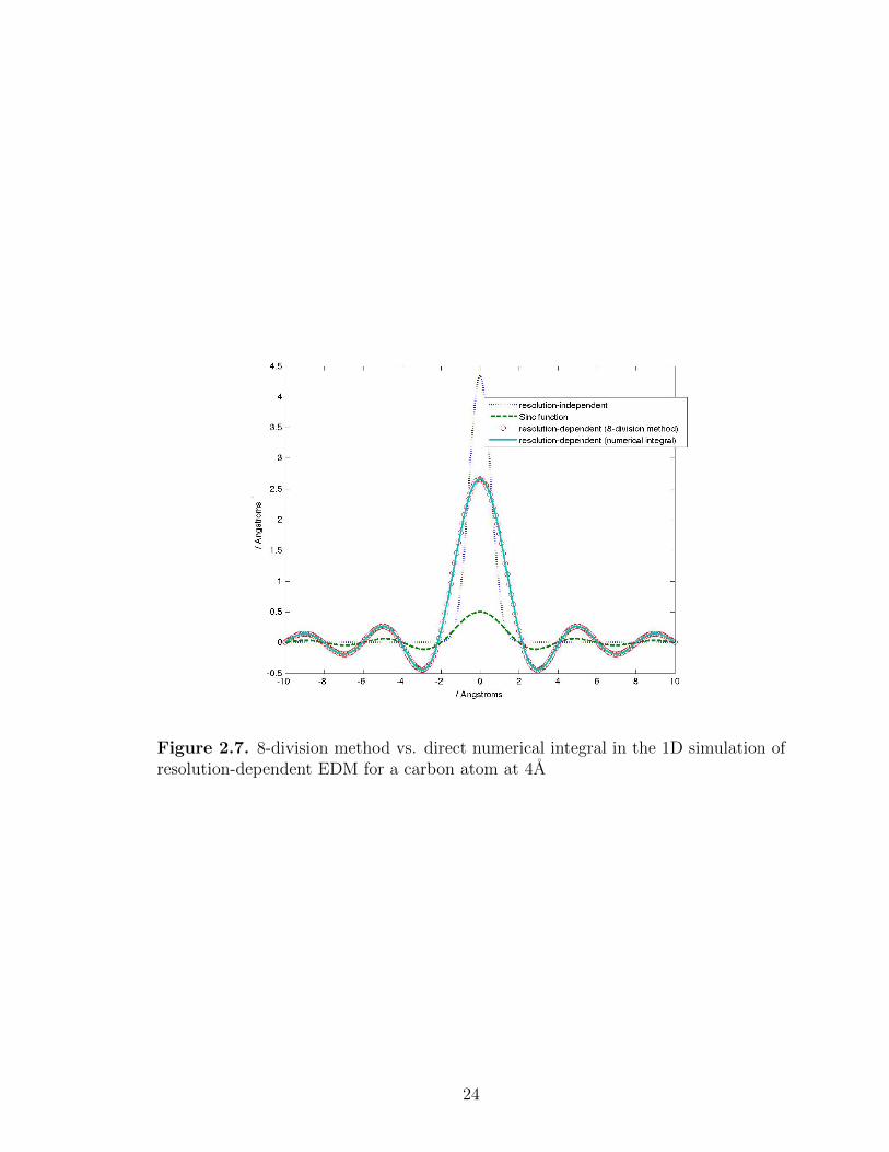
Figure 2.7. 8-division method vs. direct numerical integral in the 1D simulation ofresolution-dependent EDM for a carbon atom at 4A

24

CHAPTER 3

ERROR DISTRIBUTION OFRESOLUTION-DEPENDENT ELECTRON DENSITIES

Regarding the side chain assignment using X-ray data, we must always choose

the best-fit side chain conformation from a number of choices (e.g. rotamers). To

score each choice, we should compare the modeled resolution-dependent EDM (see

Section 2.3) against the observed EDM according to some particular error distribu-

tion.

In Section 3.1, we use DFT to represent the relationship between structure factors

and electron density values. Although continuous Fourier series (CFS) is widely used

to compute an EDM from observed structure factors, we use the DFT relationship in

a novel way to also compute the error propagation from observed structure factors to

the resolution-dependent electron density values.

When we perform a DFT, sampling the continuous electron density function to

a discrete one will create periodic replicas of the original spectrum repeated at the

reciprocal-space grid points, resulting in aliasing or overlapping of the spectrum in

the reciprocal domain. So, working with a DFT without aliasing requires us to choose

the sampling frequency to at least the Nyquist’s frequency. However, if the sampling

frequency is too high, we will see in Section 3.2, there will be many redundant ze-

ros in the reciprocal space, correlating the electron density values at different points

in the real space. To address aliasing and also avoid correlation between resolution-

dependent electron density values, we require two steps: first, we choose the sampling

frequency to be the Nyquist frequency, and second, we use a cubic filter as described

25

in (2.14). Then, by assuming all the real and imaginary parts of the structure fac-

tors are independent and identically-distributed (i.i.d.) Gaussian and noting DFT is

a unitary transformation, we conclude the measured resolution-dependent electron

density values are i.i.d. Gaussian as well. This property in turn, transforms the lo-

cal structure refinement into a maximum-likelihood problem that can be solved by

least squares (Section 3.3). Finally, in Section 3.4, we perform decision-makings for

SCA problem using X-ray data only, and present the calculation of the confidence

probability.

3.1 Discrete Fourier Transform (DFT) Representation

The well known relationships (2.3) and (2.4) between electron densities and struc-

ture factors are rewritten by the following formula pair:

ρ(x, y, z) =1

XY Z

∑hkl

Fhkle−j2π(h x

X+k y

Y+l z

Z) (3.1)

Fhkl =

∫∫∫V

ρ(x, y, z)ej2π(h xX

+k yY

+l zZ

)dx dy dz (3.2)

where ρ(x, y, z) is the electron density at position vector ~r = (x, y, z) and X, Y, Z are

the lengths of the unit cell’s edges.

This representation is conventionally known as discrete Fourier transform (DFT)

[6]. Here we will clarify the confusion between continuous Fourier series (CFS) and

DFT. The crystal can be considered as a convolution of one unit cell’s electron den-

sity function and a lattice of delta functions, with the spacing between lattice grid

points being equal to the dimension of unit cell. The real-space convolution implies

a reciprocal-space multiplication. Once the product of the two Fourier domain com-

ponents is obtained, by applying inverse Fourier transform, we have the above (3.1).

The inclusion of 3D lattice makes the summation look like a DFT. However, by refer-

ring to the theory of Digital Signal Processing (DSP), we know that (3.1) and (3.2)

26

are respectively the synthetic and analytic equations of Continuous Fourier Series

(CFS). In fact, the sampled or discretized lattice in CFS is over the 3D crystal, while

the DFT sampling grid is within a single unit cell of the given crystal. That is the

fundamental difference between these two concepts.

In DSP theory, (3.1) and (3.2) are the standard definitions of 3D CFS. The exact

definitions of Continuous Fourier Transform (CFT) is given in (3.3), Discrete-time

Fourier Transform (DTFT) in (3.4), and Discrete Fourier Transform (DFT) in (3.6)

as follows.

ρ(x, y, z) =1

XY Z

1

(2π)3

∫∫∫FCFT (Ωx,Ωy,Ωz)e

−j(Ωx x+Ωy y+Ωz z) dΩx dΩy dΩz

FCFT (Ωx,Ωy,Ωz) = XY Z

∫∫∫ρ(x, y, z)ej(Ωx x+Ωy y+Ωz z)dx dy dz (3.3)

ρ[nx, ny, nz] =1

XY Z

1

(2π)3

∫∫∫FDTFT (ωx, ωy, ωz)e

−j(ωx nx+ωy ny+ωz nz) dωx dωy dωz

FDTFT (ωx, ωy, ωz) = XY Z∞∑

nx=−∞

∞∑ny=−∞

∞∑nz=−∞

ρ[nx, ny, nz]ej(ωx nx+ωy ny+ωz nz) (3.4)

ρ[nx, ny, nz] =1

XY Z

1

NxNyNz

Nx−1∑kx=0

Ny−1∑ky=0

Nz−1∑kz=0

FDFT [kx, ky, kz]e−j( 2πkx nx

Nx+

2πky nyNy

+ 2πkz nzNz

)

FDFT [kx, ky, kz] = XY ZNx−1∑nx=0

Ny−1∑ny=0

Nz−1∑nz=0

ρ[nx, ny, nz]ej( 2πkx nx

Nx+

2πky nyNy

+ 2πkz nzNz

)(3.5)

where ρ[nx, ny, nz] = ρ(nx∆x, ny∆y, nz∆z) is the sampled discrete version of the con-

tinuous function, ρ(x, y, z), and ∆x,∆y,∆z are the sampling intervals along x−, y−, z−

axes. By definition, we have ∆x = XNx

, and similarly for ∆y and ∆z. It is clear from

the above formulation that the summation in DFT is different from the one in CFS.

27

Note all the above equations are defined for the resolution-independent EDM.

As for the resolution-dependent EDM, these relationships are the same except that

the structure factors are truncated by the limiting sphere/cube. Because the discrete

resolution-dependent EDM can easily be stored in digital devices as a discrete function

over 3D grid, it is desirable to study the relationship between structure factors and

electron density values in a discrete case, i.e. the DFT representation. Furthermore,

the DFT can be implemented efficiently using an FFT.

ρ[nx, ny, nz, Dmin] =1

XY Z

1

NxNyNz

Nx−1∑kx=0

Ny−1∑ky=0

Nz−1∑kz=0

FDFT [kx, ky, kz]e−j( 2πkx nx

Nx+

2πky nyNy

+ 2πkz nzNz

)

FDFT [kx, ky, kz] = XY ZNx−1∑nx=0

Ny−1∑ny=0

Nz−1∑nz=0

ρ[nx, ny, nz, Dmin]ej( 2πkx nx

Nx+

2πky nyNy

+ 2πkz nzNz

)

(3.6)

where ρ[nx, ny, nz, Dmin] is the sampled discrete version of the continuous function,

ρ(x, y, z,Dmin), and the symbol “ˆ” represents that the DFT coefficients are related

to the convolved resolution-dependent EDM, ρ(x, y, z,Dmin), as defined in (2.7) and

numerically computed by (2.16).

The resolution-dependent electron density function is 3D periodic over the crys-

tal. We already have its CFS given in (2.8), and CFT in (2.9). After sampling,

ρ(x, y, z,Dmin) is discretized to ρ[nx, ny, nz, Dmin], and thus can be used to compute

DTFT and DFT.

From DSP theory, we have the following relationships between Fourier transforms

and Fourier series:

FCFT (Ωx,Ωy,Ωz) =∞∑

h=−∞

∞∑k=−∞

∞∑l=−∞

(2π)3 Fhklδ(Ωx − h2π

X)δ(Ωy − k

2π

Y)δ(Ωz − l

2π

Z)

(3.7)

28

FDTFT (ωx, ωy, ωz) =1

∆x∆y∆z

∞∑h=−∞

∞∑k=−∞

∞∑l=−∞

FCFT (ωx − 2πh

∆x,ωy − 2πk

∆y,ωz − 2πl

∆z)

(3.8)

FDTFT (ωx, ωy, ωz) =∞∑

h=−∞

∞∑k=−∞

∞∑l=−∞

(2π)3

NxNyNz

FDFT [h, k, l]δ(ωx−h2π

Nx

)δ(ωy−k2π

Ny

)δ(ωz−l2π

Nz

)

(3.9)

Substituting (3.7) into (3.8) and comparing with (3.9), the relationship between

CFS and DFT can be written as

FDFT [h, k, l] = NxNyNz

∞∑m=−∞

F(h+mNx)(k+mNy)(l+mNz), (3.10)

where “ˆ” means the structure factors are truncated by the limiting sphere as in

(3.6). Specifically, for the spherical filter,

Fhkl =

Fhkl, if ( h

X)2 + ( k

Y)2 + ( l

Z)2 ≤ r2

`

0, otherwise;

(3.11)

while for a cubic filter,

Fhkl =

Fhkl, if | h

X|, | k

Y|, | l

Z| ≤ r√

2< r`

0, otherwise.

(3.12)

The problem of aliasing appears apparently in (3.10), which was first demon-

strated for reciprocal-space structure refinements in [4] and [28]. To avoid aliasing,

an imaginary thermal factor, i.e. B-factor, is included to make the spectrum shrink.

In our problem, the reciprocal-space components, Fhkl’s, are already truncated by the

29

limiting sphere as in (2.12). As long as we make the sampling grid fine enough, those

infinitely many periodic replicas of Fhkl cannot overlap. In other words, the sampling

frequency should satisfy Nyquist’s criterion, given by

Ωc ·∆x ≤ π

Ωc ·∆y ≤ π

Ωc ·∆z ≤ π (3.13)

or

∆x ≤ Dmin

2

∆y ≤ Dmin

2

∆z ≤ Dmin

2(3.14)

for the limiting sphere and

∆x ≤ Dmin√2

∆y ≤ Dmin√2

∆z ≤ Dmin√2

(3.15)

for the limiting cube.

Furthermore, if the sampling frequency is greater than or equal to the Nyquist’s

frequency, which is the least one to avoid the overlapping of spectrum, (3.10) can be

simplified as

FDFT [h, k, l] = NxNyNz Fh′k′l′ (3.16)

30

where h′ =

h, if h < Nx − h

h−Nx, otherwise,

k′ =

k, if k < Ny − k

k −Ny, otherwise,

l′ =

l, if l < Nz − l

l −Nz, otherwise.

Note for the DFT, h, k, l are integers from the intervals [0, Nx − 1], [0, Ny −

1], [0, Nz − 1] respectively.It should also be noted that Fh′k′l′ are either measured

structure factors, or constant zeros added when performing 3D DFT.

Substituting (3.16) into (3.6), we have

ρ[nx, ny, nz, Dmin] =1

XY Z

Nx−1∑h=0

Ny−1∑k=0

Nz−1∑l=0

Fh′k′l′e−j( 2πhnx

Nx+

2πk nyNy

+ 2πl nzNz

)(3.17)

Fh′k′l′ =XY Z

NxNyNz

Nx−1∑nx=0

Ny−1∑ny=0

Nz−1∑nz=0

ρ[nx, ny, nz, Dmin]ej( 2πhnx

Nx+

2πk nyNy

+ 2πl nzNz

), (3.18)

and then put (3.18) in a matrix form as

F =XY Z

NxNyNz

E ρ =1√

NxNyNz

(1√

NxNyNz

E) XY Z ρ , (3.19)

where F and ρ are column vectors including the real and imaginary parts of all of

the Fh′k′l′ ’s and ρ[nx, ny, nz, Dmin]’s respectively for 0 ≤ nx(h) ≤ Nx− 1, 0 ≤ ny(k) ≤

Ny − 1, 0 ≤ nz(l) ≤ Nz − 1. E is a 2NxNyNz × 2NxNyNz matrix, which is composed

of the real and imaginary parts of all the complex exponentials. It can be shown that

( 1√NxNy Nz

E) is a unitary matrix, denoted as A. Then a property of a unitary matrix

follows, i.e. ATA = AAT = I, where I is an identity matrix. (3.19) can be rewritten

as

F =XY Z√NxNyNz

A ρ . (3.20)

31

To verify that matrix ( 1√NxNy Nz

E) is a unitary matrix, we write down all the

entries of this matrix. A unitary matrix has any pair of different rows orthogonal and

the squared norm of each row equal to one. So we can check the inner product of

any pair of rows, say one row with index tuple (h, k, l), and the other with (H,K,L).

They can be the same, and in that case, these two rows describe a single row. It is

easy to see the inner product actually fall into two categories. Let r and r′ represent

two rows. Suppose both of them correspond to the real (imaginary) parts of two

complex structure factors, we have the inner product given as

1

NxNyNz

Nx−1∑nx=0

Ny−1∑ny=0

Nz−1∑nz=0

[cos(2πhnxNx

+2πk nyNy

+2πl nzNz

) cos(2πH nxNx

+2πK nyNy

+2πLnzNz

)

+sin(2πhnxNx

+2πk nyNy

+2πl nzNz

) sin(2πH nxNx

+2πK nyNy

+2πLnzNz

)]

=1

NxNyNz

Nx−1∑nx=0

Ny−1∑ny=0

Nz−1∑nz=0

cos(2πnxh−HNx

+ 2π nyk −KNy

+ 2π nzl − LNz

)

=1

NxNyNz

<[Nx−1∑nx=0

Ny−1∑ny=0

Nz−1∑nz=0

ej2πnx

h−HNx

+j2π nyk−KNy

+j2π nzl−LNz ]

=1

NxNyNz

<[Nx−1∑nx=0

ej2πnxh−HNx

Ny−1∑ny=0

ej2π ny

k−KNy

Nz−1∑nz=0

ej2π nzl−LNz ]

=

1, if h = H, k = K, l = L

0, otherwise.

(3.21)

If r and r′ are from the same structure factor, the inner product is one; otherwise, it

is zero.

In the other case, when we have one row from the real part of a structure factor,

and the other row from the imaginary part of a structure factor, we have

32

1

NxNyNz

Nx−1∑nx=0

Ny−1∑ny=0

Nz−1∑nz=0

[sin(2πhnxNx

+2πk nyNy

+2πl nzNz

) cos(2πH nxNx

+2πK nyNy

+2πLnzNz

)

−cos(2πhnxNx

+2πk nyNy

+2πl nzNz

) sin(2πH nxNx

+2πK nyNy

+2πLnzNz

)]

=1

NxNyNz

Nx−1∑nx=0

Ny−1∑ny=0

Nz−1∑nz=0

sin(2πnxh−HNx

+ 2π nyk −KNy

+ 2π nzl − LNz

)

=1

NxNyNz

=[Nx−1∑nx=0

Ny−1∑ny=0

Nz−1∑nz=0

ej2πnx

h−HNx

+j2π nyk−KNy

+j2π nzl−LNz ]

=1

NxNyNz

=[Nx−1∑nx=0

ej2πnxh−HNx

Ny−1∑ny=0

ej2π ny

k−KNy

Nz−1∑nz=0

ej2π nzl−LNz ]

= 0, (3.22)

which implies the inner product is constant zero no matter whether they are from the

same structure factor.

From both the cases mentioned above, we conclude the 2NxNyNz rows are or-

thonormal, so the square matrix ( 1√NxNy Nz

E) is a unitary matrix.

3.2 The Probability Distribution of Electron Densities

It is seen that by choosing sampling frequency greater than or equal to the

Nyquist’s frequency, the discrete electron densities calculated from the DFT synthetic

equation (3.17) are exactly the sampled values of the continuous resolution-dependent

EDM given in (2.7). We assume the observed complex structure factors are i.i.d. 2D

Gaussian-distributed; however, as shown later, the discrete electron densities are also

i.i.d. 2D Gaussian as long as there is no constant zero in the column vector, F . Based

on this requirement, the limiting sphere is discarded and a limiting cube along with

its implementation is presented.

The deterministic equation (3.20) can be taken as a modeled relationship, which

is overwritten as

33

F cal =XY Z√NxNyNz

A ρcal

. (3.23)

Let us consider a random scenario, which requires to study the joint probabilistic dis-

tribution of the random vector, consisting of the measured structure factors, denoted

as F obs, meaning the observed random vector.

The general distribution of individual structure factors is given by Read [30]. The

conditional error distribution of a particular structure factor given a structural model

relies on both the model’s coordinate errors and the contributions from the missing

atoms. The general distribution is a 2D Gaussian distribution, given by

Fhklobs = D(h, k, l,Dmin) Fhklcal + ε , (3.24)

where ε is a 2D Gaussian error. The mean value is

〈Fhklobs〉 = D(h, k, l,Dmin) Fhklcal .

The real and imaginary parts of ε are independent and identical-distributed (i.i.d.)

1D Gaussian random variables, with the variances equal to

σ2F = [1−D2(h, k, l,Dmin)]ΣP + ΣQ,

where ΣP and ΣQ represent the variance contributions from the known atoms in the

given model, and the missing atoms (e.g. water molecules in our problem) to be

determined, respectively. D(h, k, l,Dmin) can be complex, which implies the coor-

dinate errors of the known atoms in the model. One more note is made here that

D(h, k, l,Dmin) in Read’s work [30] is a function of the resolution, Dmin, and the

reciprocal-space coordinates, (h, k, l); however, if the resolution-dependent EDM in

Section 2.3 is used, D(h, k, l,Dmin) is not varying with the resolution.

34

We focus on the ML estimate of the structural conformations, which always max-

imizes the conditional probability of the observed data given the modeled structure,

meaning the structure is perfectly known. Also, we assume the thermal motion of the

native structure in the crystal can be ignored, compared with the wide-type struc-

tural dynamics. For these reasons, we take the atomic model for calculating modeled

structure factors as a perfect one, and all of the atomic coordinate errors can thus be

eliminated, which gives D(h, k, l,Dmin) ≈ 1. Then (3.24) is simplified as

Fhklobs = Fhklcal + ε (3.25)

with the mean 〈Fhklobs〉 = Fhklcal and the variance σ2F = ΣQ, which implies the ran-

dom errors, ε’s, for different structure factors, are identically-distributed 2D Gaussian

complex random variables with zero-mean and σ2F as the variance.

Next, we take a look at the joint probability distribution of a set of structure

factors. Klug [23] find out that the cross-correlated terms of the joint distribution

are proportional to N−1/2, where N is the number of atoms in the system. For

large molecules (e.g. proteins), containing much more than hundreds of atoms, the

correlations between different structure factors become so weak that they can be

neglected without involving much error.

Thus, given the calculated structure factors from a structural model, the real and

imaginary parts of the measured structure factors can be considered as an independent

and identically-distributed (i.i.d.) Gaussian random vector. The general distribution

is given as

F obs = F cal + ε , (3.26)

where ε is a 2NxNyNz by 1 random vector comprising with i.i.d. Gaussian entries

having zero mean, variance σ2F , along with constant zeros depending on the choice of

35

sampling frequency. Note ε is but a real vector since we put all the real and imaginary

parts of the structure factors in a vector form.

Substituting (3.23) into (3.26),

F obs =XY Z√NxNyNz

A ρcal

+ ε

= B ρcal

+ ε (3.27)

where B = XY Z√NxNy Nz

A.

The least squares (LS) estimate of ρcal

is denoted as ρobs

, and given by

ρobs

= (BTB)−1BT F obs

=

√NxNyNz

XY ZAT F obs (3.28)

where ATA = I is used.

So, according to (3.28), an observed EDM can be constructed based on the mea-

sured complex structure factors. Here it should be pointed out, the state-of-the-

art techniques can not only measure the amplitudes of structure factors, but also

the phase information through multiple isomorphous replacement (MIR) or multi-

wavelength anomalous diffraction (MAD) [31][2], which renews the general interest

in real-space refinement. Since the phase information is measured precisely, we are

not restricted to refine the amplitudes of structure factors in the reciprocal space.

Without mention of the phase measurements, for the rest of this thesis, we assume

the phase information is measured through either MIR or MAD.

(3.28) shows that the LS estimate ρobs

is a linear transformation of F obs, which

consists of i.i.d. Gaussian structure factors and constant zeros (i.e. Gaussian with

zero mean, zero variance). So we conclude the random vector ρobs

is Gaussian as well.

To describe a Gaussian random vector, there are two parameters: the mean vector

and the covariance matrix.

36

The mean vector of ρobs

is

〈ρobs〉 =

√NxNyNz

XY ZAT 〈F obs〉

=

√NxNyNz

XY ZAT

XY Z√NxNyNz

A ρcal

= ρcal

, (3.29)

and the covariance matrix is given by

Σ = E[(ρobs− 〈ρ

obs〉)(ρ

obs− 〈ρ

obs〉)T ]

= E[(

√NxNyNz

XY ZAT F obs −

√NxNyNz

XY ZAT F cal)

(

√NxNyNz

XY ZAT F obs −

√NxNyNz

XY ZAT F cal)

T ]

=NxNyNz

(XY Z)2ATE[(F obs − F cal)(F obs − F cal)

T ]A

=NxNyNz

(XY Z)2ATE[ε εT ]A . (3.30)

From (3.30), it is obvious that the covariance matrix of ρobs

depends mainly on

the covariance matrix of ε. As we discussed, ε is comprised with i.i.d. Gaussian

structure factors and constant zeros. For the reason stated below, it is not desired to

have constant zeros in ε, i.e. the probabilistic distributions of all the entries of ε are

consistent.

Due to the truncation of structure factors by the limiting sphere, after perform-

ing 3D DFT, we have periodic replicas of the spherical spectrum repeated at the

reciprocal-space grid points. Fig. 3.1(a) illustrates the resulting spectrum in a period

box. The white sphere is the original spectrum filtered through the limiting sphere,

and the black parts from different spheres are the periodic replicas within the period

box.

For the case of the spherical filter (i.e. the limiting sphere), if the Nyquist’s

frequency is exactly selected, the black parts from different spheres will be drawn close

37

(a) Sphere-case DFT within one period box in reciprocal space

(b) Cube-case DFT within one period box in reciprocal space

Figure 3.1. Comparisons of 3D DFT results between spherical and cubic filters

38

such that their surfaces just intersect. However, because those parts obey spherical

symmetry, there will still be many constant zeros around the center of the given

period box. This can be addressed by replacing the spherical filter with a cubic filter.

The DFT spectrum pertaining to the cubic filter in the period box is illustrated in

Fig. 3.1(b).

It is obvious that by choosing the Nyquist’s frequency, the black parts from dif-

ferent cubes will touch the faces of each other, and there will be no constant zeros

among the entries of ε.

To realize the cubic filter, we can eliminate the structure factors near the surface

of the limiting sphere, forming a maximum cube enclosed by the limiting sphere.

This treatment will definitely degrade the constructed EDM, since we are using fewer

structure factors. However, this allows us to analyze the error distribution of electron

densities in a simply way, and by selecting the maximum cube, it is also expected the

quality of the so-constructed EDM should be fine.

Using the cubic filter and the Nyquist’s frequency, ε is comprised of pure i.i.d.

zero mean, σ2F variance Gaussian random variables, which means E[ε εT ] = σ2

F I (I

is an identity matrix). We can rewrite (3.30) as

Σ =NxNyNz

(XY Z)2ATσ2

F IA

=NxNyNz

(XY Z)2σ2FA

TA

=NxNyNz

(XY Z)2σ2F I

= σ2ρI (3.31)

where σ2ρ = NxNy Nz

(XY Z)2σ2F . (3.31) implies the covariance matrix of the random vector,

ρobs

, is constant times an identity matrix; or equivalently, the electron densities of the

measured EDM are i.i.d. Gaussian as well. This statistical result comes from the use

of the cubic filter and the Nyquist’s sampling frequency.

39

We make a note here, since we cannot measure F000obs in an X-ray experiment,

the covariance matrix of ρobs

cannot be perfectly constant times an identity matrix;

however, the exact result is Σ = NxNy Nz(XY Z)2

σ2F I, where the diagonal entries of I are

NxNy Nz−1

NxNy Nz’s, and all the other entries are −1

NxNy Nz’s. As the number of samples is

much larger than one, we are confident to make the following approxiamtion Σ ≈NxNy Nz(XY Z)2

σ2F I = Σ.

The reason that it is desired to have the entries of ρobs

independent or uncorrelated,

is illustrated in Fig. 3.2.

In this example, we demonstrate the effect of correlation in a 1D carbon atom’s

electron densities. We assume the carbon atom is Gaussian-distributed with the

standard deviation 0.55A and 6 electrons spreading around the nuclei. The dimension

size of this 1D simulated unit cell is 50A, and the resolution is 2.5A, meaning the

maximum reciprocal-space index of the measured structure factors is 502.5

= 20. For

the situation at the Nyquist’s sampling frequency, there are 2×20+1 = 41 samples in

one unit cell. We generate i.i.d. Gaussian random errors (zero mean and 102 variance)

among the 40 measured structured factors, and the reconstructed EDM by performing

41-point DFT is shown in Fig. 3.2(a). Since the errors among the reconstructed EDM

are uncorrelated and identical, we can easily find out that the scattered points are

independent of each other, and bounded by ±σρ = ±√NxXσF = ±

√41

5010 = ±1.64A−1

around the true electron density curve. This bound is taken as a noise bound, within

which the electron densities are totally unreliable. It is also implied that the sub-

peaks in the noise bound cannot be counted as possible atomic centers, reducing the

risk of overfitting. Furthermore, by taking the noise bound into account, we can fit

a modeled electron density function to data very easily since the data is believed

to deviate from the modeled function by σρ. For comparison, we also show the

over-sampled case as in Fig. 3.2(b) with 1000 samples in the same simulated unit

cell. By using the same Gaussian error distribution and adding 1000 − 41 = 959

40

(a) uncorrelated errors at Nyquist’s frequency with 41 samples in the unit cell

(b) correlated errors with 1000 samples in the unit cell

Figure 3.2. 1D simulation of EDM measurements

41

constant zeros in the DFT, the errors among the electron density values are strongly

correlated. Since the electron density values are not i.i.d. any more in this case, there

is no such a uniform noise bound confining the unreliable density values. As a result,

fitting a modeled electron density function to the measurements also becomes difficult.

Another important application of an uncorrelated EDM is to calculate the confidence

probability for decision-makings in real-space refinement (see Section 3.4.2).

3.3 Statistical Properties

As discussed in Section 3.2, if we choose the Nyquist’s frequency and the cubic

filter, all of the entries in ρobs

are i.i.d. Gaussian. Note ρobs

is composed of the real

and imaginary parts of all the electron densities in the unit cell. Since the mean

value of the electron density is a pure real number, we can only take the real parts in

ρobs

. Thus we conclude the so-constructed electron densities (i.e. a subset of entries

in ρobs

), are still i.i.d. Gaussian. In other words, the error distribution is equivalent

for all the sampled density points in the observed EDM, and the variance is not a

function of the position in the unit cell.

3.3.1 Maximum Likelihood (ML) estimate of protein structures

Given a calculated EDM model, the conditional probability distribution function

(pdf) of an observed EDM, is

f(ρobs| ρ

cal) =

1

(√

2π)NxNyNzdet(Σ)e−

12

(ρobs−ρ

cal)TΣ−1(ρ

obs−ρ

cal)

=1

(√

2π σ2ρ)NxNyNz

e−12

(ρobs−ρ

cal)TΣ−1(ρ

obs−ρ

cal)

=1

(√

2π σ2ρ)NxNyNz

e− 1

2σ2ρ(ρobs−ρ

cal)T (ρ

obs−ρ

cal)

(3.32)

42

where Σ −1 = 1σ2ρ

1 0 · · · 0

0 1 · · · 0

......

. . ....

0 0 · · · 1

.

Let us define Θ as the conformational space. The Maximum Likelihood (ML)

estimate of a structural conformation c is formulated as

c∗ = arg maxc∈Θ

f(Local EDM data around c | c)

= arg maxc∈Θ

f(ρobs| ρ

cal(c))

= arg maxc∈Θ

1

(√

2π σ2ρ)NxNyNz

e− 1

2σ2ρ(ρobs−ρ

cal(c))T (ρ

obs−ρ

cal(c))

= arg minc∈Θ

(ρobs− ρ

cal(c))T (ρ

obs− ρ

cal(c))

= arg minc∈Θ‖ρ

obs− ρ

cal(c)‖2 (3.33)

where ρcal

(c) is the resolution-dependent EDM calculated (see Section 2.3) around

the local region of the conformation c.

(3.33) implies the ML structural estimate can be expressed as a Least Squares

(LS) solution. An application of this ML estimate is to determine the local structure

using local EDM, such as side chain assignment, which is discussed in Section 3.4.

3.3.2 Discrete-case Parseval’s Theorem

The widely-used description of the real-space fitting error is the mean square error

(MSE) of the whole EDM, which is derived from Parseval’s Theorem [31]. However,

it is a score for the entire EDM, but not for individual sampled density points. Our

framework is capable of obtaining the error distribution of the electron density at

each sampled point, as shown in Section 3.2. Next, we will show our framework can

also handle the Parseval’s theorem (i.e. MSE score), which is in a discrete sense.

43

We use the above formulation to derive the discrete-case Parseval’s theorem.

ρobs

=

√NxNyNz

XY ZAT F obs

ρcal

=

√NxNyNz

XY ZAT F cal

ρobs− ρ

cal=

√NxNyNz

XY ZAT (F obs − F cal)

(ρobs− ρ

cal)T (ρ

obs− ρ

cal) = (

√NxNyNz

XY Z)2( F obs − F cal)

T AAT ( F obs − F cal)

‖ρobs− ρ

cal‖2 = (

√NxNyNz

XY Z)2 ‖ F obs − F cal‖2 (3.34)

where “‖ · ‖” is the Euclidean norm of a vector. We have used many times the fact

that if A is a unitary matrix, AT A = AAT = I, where I is an identity matrix.

Both the observed EDM and the modeled EDM are constructed in the same way to

compare with each other. The squared norm of deviation in (3.34) is a widely-used

measure of the EDM fitting.

3.4 Decision Making and Confidence Probability

We show the problem of protein side chain assignment (SCA) as an example of

performing local real-space refinement. For each amino acid residue, there are finitely

many possible side chain conformations, called rotamers. Assuming the backbone and

the observed EDM are given, for each residue, a best-fit rotamer can be determined

44

according to the Maximum Likelihood decision rule. There is definitely uncertainty of

making this decision. We define a measure of uncertainty or equivalently, confidence

probability, and also propose a numerical way to calculate it.

3.4.1 Decision Rules for Refinement

Let us assume the real-space refinement is performed over a discrete conformation

space, e.g. side chain rotamers. It is shown that the ML estimate reduces to a LS

solution in Section 3.3.1, which requires to compute the squared Euclidean norm of

the density difference vector as a matching score. We postulate that the rotamer with

the smallest matching score is the best-fit rotamer.

Decision Rule 1. For each amino acid residue, there are N possible side chain

rotamers. The rotamer set is denoted as r1, . . . , rN. Provided that the backbone

is determined, and the local EDM is obtained from an X-ray experiment, the ML

estimate of the side chain structure can be selected by the following rule:

If

f(Local EDM data around rk | rk) > f(Local EDM data around ri | ri)

for i = 1, 2, . . . , N, i 6= k, rotamer rk is then selected.

From (3.32), the ML estimate is equivalent to the LS solution. Thus, we define

the squared norm of the difference, between the observed electron density vector ρobs

and the calculated vector ρcal

(rk), as the matching score, denoted by Rk. Then, we

have the following LS decision rule.

Decision Rule 2. For each rotamer from the rotamer set, a modeled local EDM can

be constructed. If the backbone is fixed and the observed EDM is obtained from an

45

X-ray experiment, we compute the matching scores for all the N rotamers. The ML

estimate of the side chain structure is rk, if

‖ρobs− ρ

cal(rk)‖2 < ‖ρ

obs− ρ

cal(ri)‖2 for i = 1, 2, . . . , N, i 6= k,

or Rk < Ri for i = 1, 2, . . . , N, i 6= k. (3.35)

3.4.2 Confidence Probability Calculation

According to the LS decision rule, the rotamer with the smallest matching score

is always preferable, called the best-fit rotamer. So the confidence probability of the

decision-making relies on the statistics of these matching scores. We first study the

probability distribution of the matching scores, and then develop a numerical way to

calculate the confidence probability.

Let us take a look at the general distribution of the matching scores. For a rotamer

ri of a particular residue, suppose the local EDM around the side chain structure has

M sampled density points. The observed electron density vector ρobs

is the calculated

electron density vector of the native side chain conformation plus i.i.d. zero-mean, σ2ρ-

variance Gaussian errors. Vector ρcal

(ri) is calculated using ri as a structural model

of the side chain.

ρobs

= ρcal

(Native) + ερ

So the difference vector is given by

ρobs− ρ

cal(ri) = [ρ

cal(Native)− ρ

cal(ri)] + ερ ,

and the matching score is thus the squared Euclidean norm of this difference vector,

which is

46

Ri = ‖ρobs− ρ

cal(ri)‖2 . (3.36)

In another word, Ri is just a sum of M squared Gaussian random variables. Precisely,

Ri is a sum of M χ2 random variables. In practice, we have M greater than 100, so by

Central Limit Theorem, the summation of χ2 random variables can be approximated

as a single Gaussian random variable. It can be shown that, by utilizing the moments

of Gaussian random variables, the mean and the variance of Ri are listed as

E[Ri] = ‖ρcal

(Native)− ρcal

(ri)‖2 +Mσ2ρ

V ar[Ri] = 4σ2ρ‖ρcal(Native)− ρcal(ri)‖

2 + 5Mσ4ρ , (3.37)

where ‖ρcal

(Native) − ρcal

(ri)‖2 comes from the coordinate errors of the structural

model ri, and σ2ρ is the 2D Gaussian random error due to the missing atoms in the

model.

Next, we compute the confidence probability that, the best-fit rotamer returned

by the decision rule is coincidentally the best rotamer, which is defined as the closest

rotamer (i.e. minimum all-atom deviation) to the native side chain structure. Note it

is not always the best. Suppose the kth rotamer rk is the closest rotamer to the native

conformation. If we desire to choose this rotamer in the local real-space refinement,

according to the LS decision rule, we should have the following condition:

Rk < Ri, for i = 1, 2, . . . , N, i 6= k. (3.38)

So the confidence probability is the probability that (3.38) holds, denoted as P (Rk <

Ri, for i = 1, 2, . . . , N, i 6= k). Noting all the matching scores are conditionally

independent Gaussian random variables with the means and the variances specified

in (3.37), the confidence probability can thus be calculated as

47

P (Rk < Ri, for i = 1, 2, . . . , N, i 6= k)

=

∫ ∞∞

f(Rk = x)P (Ri > Rk, for i = 1, 2, . . . , N, i 6= k|Rk = x) dx

=

∫ ∞∞

f(Rk = x)P (Ri > x, for i = 1, 2, . . . , N, i 6= k) dx

=

∫ ∞∞

f(Rk = x)∏

i=1,2,...,N

i 6=k

P (Ri > x) dx

=

∫ ∞∞

f(Rk = x)∏

i=1,2,...,N

i 6=k

[1− Φ(Ri < x)] dx

≈∫ E[Rk]+3σRk

E[Rk]−3σRk

f(Rk = x)∏

i=1,2,...,N

i 6=k

[1− Φ(Ri < x)] dx . (3.39)

where σRk =√V ar[Rk], and Φ(Ri < x) is the cumulative distribution function (cdf)

of the Gaussian random variable Ri. The last step uses the 3σ rule [44] of a Gaussian

random variable. For the remaining integral, we can still make use of the 8-division

method, which proves to be an efficient numerical method.

48

CHAPTER 4

EXPERIMENTAL RESULTS USING X-RAY DATA ONLY

In Section 3.4.1, two decision rules, i.e. ML and LS, are demonstrated. Because of

the Gaussian random errors, the two rules are equivalent to each other. We need to

validate this probabilistic model for X-ray, and test it over several proteins of varying

resolutions.

Specifically, given a candidate rotamer, we use our forward model (2.16) to gen-

erate modeled local EDM’s. For the current rotamer, the error model in Section 3.3

is then utilized to compute the difference between the model and the observation

within the voxel of a single residue. Each rotamer choice thus has a matching score

in accordance with the squared Euclidean norm of the difference. The smaller the

difference is, the higher matching score.

We run the above algorithm over the following set of proteins at different resolu-

tions. From Table 4.1, it is easy to see that our test set is not biased, since there are

lots of residues from both α helices and β sheets. The tendency of the total accuracy

from high-quality EDM’s to poor-resolution EDM’s seems reasonable as well.

For the measure of accuracy, we define the best rotamer as the closest rotamer

choice to the known structure, which has the minimum all-atom mean square devi-

ation from the known structure as in Section 3.4.2. If the best-fit rotamer with the

highest matching score is coincidentally the best rotamer, we say that this side chain

conformation is predicted correctly. Otherwise, the prediction is incorrect.

Fig. 4.1 illustrates the accuracy for each type of amino acid at varying resolutions.

Generally speaking, the better the resolution is, the more accurate prediction results.

49

Note for Arginine (ARG) and Lysine (LYS) have long side chains, which have all of

the four χ angles, hence are difficult to predict.

Figure 4.1. Accuracy of the Prediction at Different Resolutions

The accuracy of the residue type MET at 1.5A is low because the number of

samples is small, i.e. there are only five MET residues at 1.5A resolution in our data

set.

The limitation of the decision-making based on X-ray only is the failure of ad-

dressing the clashes for long side chain residues (e.g. LYS and ARG). Fig. 5.3 is

an illustration of clashes. The best-fit rotamer choice mistakingly orients the long

Test ProteinsPDB codes resolution # of residues # in α helices # in β sheets accuracy

2wfi 0.75A 179 23 57 98.3%

3iv4 1.5A 112 55 28 95.9%

2wlw 1.5A 165 23 57 94.2%

2we2 1.5A 286 11 124 89.5%

2wiq 2.0A 259 15 119 89.84%

3fjb 2.0A 146 9 55 88.43%

2zr4 2.0A 163 39 36 78.74%

3hb0 2.5A 274 145 28 86.7%

3imq 2.5A 141 102 0 79.5%

3hjt 2.5A 287 119 44 78.5%

Table 4.1. Resolution, secondary structures and accuracy of the tested proteins

50

side chain overlapping the neighbor residue. It can also be seen that, the electron

densities around the best side chain are harder to be detected than those around the

backbone. This shows the prediction of side chain conformation (i.e. SCA problem)

is a challenging one and more difficult than the backbone determination.

Figure 4.2. The clash occurred in high-quality EDM between LYS and its neighborresidue

The confidence probability calculations are shown in Fig. 4.3. The trend of the

confidence probabilities for all types of amino acid is consistent with the accuracy

variations. It should be noted that, the values of the confidence probabilities are not

exactly correct, since we assume the matching scores are Gaussian variables with the

means and variances given in (3.37), which is mainly because the sampled electron

density points are Gaussian as well. However, the EDM’s we used for these results

are from Uppsala Electron Density Server (EDS) [22], which are not constructed us-

ing the cubic filter and the Nyquist’s frequency (see Chapter 3). The future work is

to construct our own EDM’s and then perform real-space refinement. Regarding to

the use of the confidence probability measure, we propose to run this algorithm for

the solved high-quality structures, and then generate another Ramachandran map

51

for each residue type, which stores the information of the confidence probability. We

expect the confidence probability to vary with the amino acid type and the backbone

dihedral angles (φ, ψ). This Ramachandran map tells us how reliable the side chain

conformation can be resolved using X-ray data only. By referring to the map, we sug-

gest crystallographers interpret the unreliable X-ray data meticulously and combine

additional sources of data (see Chapter 5).

52

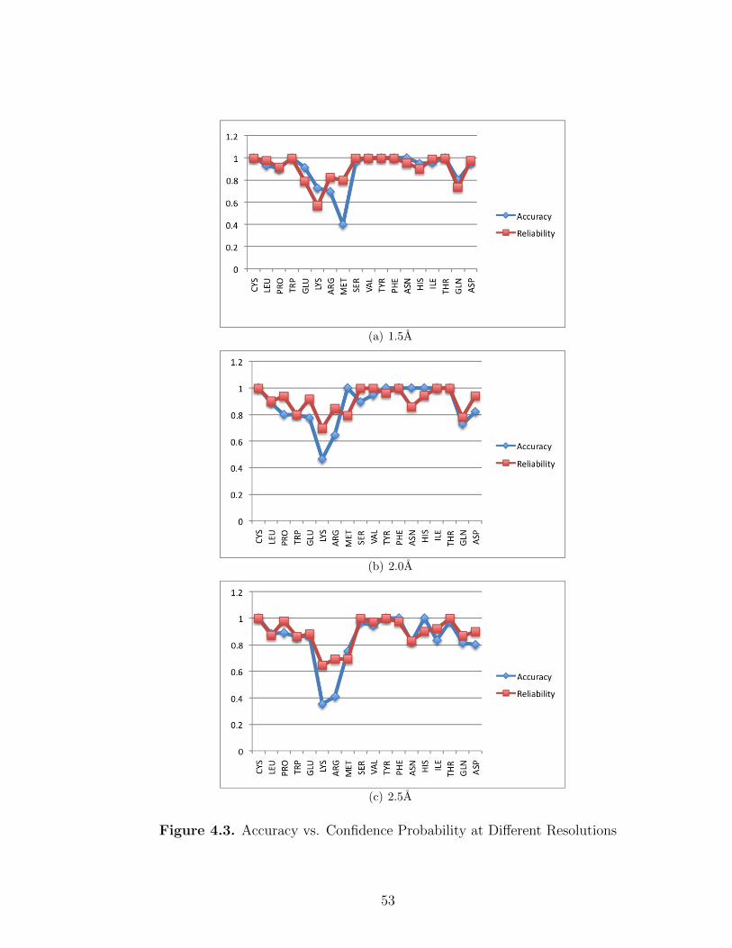
(a) 1.5A

(b) 2.0A

(c) 2.5A

Figure 4.3. Accuracy vs. Confidence Probability at Different Resolutions

53

CHAPTER 5

DATA FUSION FOR PROTEIN SIDE CHAINASSIGNMENT

We propose a framework to fuse different sources of data for the protein SCA

problem. Two essential types of data sources, i.e. NMR and potential energy, are

validated in Section 5.1. A data fusion model based on Bayesian inference is presented

in Section 5.2, with illustration of the improved prediction results.

5.1 Validation of Multiple Sources of Information

In Chapter 4, it is shown that, for long side chain residue types (e.g. ARG and

LYS), the clashes between nearby residues cannot be resolved. From this perspective,

we need to add more pairwise restraints detecting and thus eliminating the clashes.

There are two possible data sources, one of which is Nuclear Magnetic Resonance

(NMR) and the other is stereochemistry (e.g. potential energy calculation).

5.1.1 Nuclear Magnetic Resonance (NMR)

Nuclear Overhauser Effect Spectroscopy (NOESY), which is a specific NMR ex-

periment, provides us distance restraints between atoms from different residues or

within the same residue. Habeck et al. introduced a Bayesian inference method [16],

which can be incorporated into our probabilistic framework by considering the pair-

wise restraints as joint probability terms. Here is an example of how we utilize NMR

data to correct the errors, caused by the prediction using X-ray data only.

Example 1. We select ubiquitin with both X-ray and NMR data available. By running

the LS decision-making algorithm using X-ray data only, we have the 51st residue (i.e.

54

GLU) in chainA predicted incorrectly with the χ1 angle rotated 108. By searching

for the effective pairwise distance restraints between the 51st residue and the nearby

residues, we have the following data script in the NMR Restraint Grid of ubiquitin

(see Fig. 5.1). The distance between the Cγ atom of the 51st residue (GLU) and

Figure 5.1. Data Script of Ubiquitin NMR Restraint Grid

the Cγ atom of the 54th residue (ARG) is 4.870 ± 1.218 with the minimum Van der

waals distance 3.070 [34]. The side chain of the 54th residue (ARG) is correctly

predicted. Through calculation, the distance between Cγ’s respectively from the best

rotamer of GLU and ARG’s side chain is 4.944; while the distance between Cγ’s

from the best-fit rotamer of GLU and ARG’s side chain is 5.157. So the incorrectly

predicted (i.e. best-fit) rotamer has worse NMR matching score than the best rotamer,

although the difference is quite small. This is illustrated in Fig. 5.2, which shows the

above distances are actually very close to each other.

From Example 1, we know the NMR distance restraints can be incorporated as

pairwise constraints. However, there are very few effective distance restraints in NMR

data. In Example 1, the distance restraint is not very effective, either. So NMR data is

quite useful in resolving the large-scale or macromolecular structure, but not sensitive

to the side chain conformations. Researchers have to use other sources of data, e.g.

the geometrical restraints or the physical laws, to correct the prediction errors caused

by the X-ray data, e.g. to fully and confidently eliminate the clashes.

5.1.2 Potential Energy Calculation

In physics, it is believed that the natural stable structure should minimize the

total potential energy. As a result, the clashes can be avoided by searching for the

global energy minimum. For protein structures, there are several types of potential

55

Figure 5.2. The Best Rotamer vs. the Best-fit Rotamer of GLU with the distancebetween GLU’s Cγ and the nearby ARG’s Cγ

energy function, e.g. Amber, CHARMM, etc. The widely used Amber potential is

given by [43]

V (rN) =∑bonds

1

2kb(l − l0)2 +

∑angles

1

2ka(θ − θ0)2 +

∑torsions

1

2Vn[1 + cos(nω − γ)] +

N−1∑j=1

N∑i=j+1

εi,j

[(σijrij

)12

− 2

(σijrij

)6]

+qiqj

4πε0rij

(5.1)

The fourth additional term is Van der Waals potential energy function. For sim-

plicity, we only use this potential energy component to indicate the distances between

different atomic groups. Since, in physics, potential energy is calculated based on pair-

wise interactions among the charges, for describing the potential energy of the entire

protein, we can group those pairwise interactions into self-energy terms within indi-

vidual amino acids and pairwise-energy terms between different amino acids. These

energy terms are then converted to the prior probabilities using Boltzmann distribu-

tion [41].

56

Boltzmann distribution says that, if there are k conformational states in the con-

formation space Θ, the probability of the kth state is in the negative exponential form

with respect to the relative potential energy of that state.

P (statek) =e−(Ek−Emin)/RT∑Nk=1 e

−(Ek−Emin)/RT(5.2)

where R = 8.31 J/(mol ·K) is the molar ideal gas constant and T is the temperature

in kelvins (K). The denominator serves as a normalization factor, called the partition

function. The smaller the relative potential is, the higher probability the state is

observed.

Example 2. We select the 82nd residue (LYS) from our test protein with pdb code

“2zr4”. By running the LS decision-making algorithm using X-ray data only, we have

a wrong prediction, and the best rotamer ranks the fourth in the descending best-fit

rotamer list. The top three best-fit rotamers are illustrated in Fig. 5.3. In Fig. 5.3,

the HIS residue is shown to the left, while the LYS residue is displayed to the right

and outlined by the green lines. The yellow lines indicate where the clashes occur and

the associated potential energies are extremely large.

For comparison, the best rotamer is shown in Fig. 5.4.

It is obvious that the clashes occur for the top three best-fit rotamer choices, and

all of them conflict with the same HIS residue (id:64). By calculating the pairwise-

energies between the LYS rotamers and the HIS side chain, the energy values are

22867863.901, 5.27423866577×1012, 544270475.454 and −1.84317088814 respectively

with unit KJ/mol, which demonstrates the energy for the best rotamer is extremely

smaller than the energies for the clashing best-fit rotamers. This example validates the

incorporation of the potential energy as a useful data source to eliminate the clashes.

57

(a) The first best-fit rotamer

(b) The second best-fit rotamer

(c) The third best-fit rotamer

Figure 5.3. The top three best-fit rotamers of LYS residue (id: 82) in pdb file “2zr4”

58

Figure 5.4. The fourth best-fit (also the best) rotamer of LYS residue (id: 82) inpdb file “2zr4”

The question is how to fuse all three sources of data in a reasonable way. By

combining the X-ray and NMR data in the form of likelihood, and the potential energy

as a prior, it is easy to formulate the Maximum a posteriori (MAP) estimation.

5.2 Data Fusion Schemes

The goal of our work is to combine different sources of experimental data and

modeling data to firstly solve the SCA problem and then the entire protein structure.

Usually, there are two schemes for data fusion. One is named the pre-detection fusion,

as shown in Fig. 5.5(a). The likelihood functions of multi-sources of data are combined

together as a weighted joint likelihood. The weights are assigned according to the

reliability of each data source. The other scheme (i.e. decision fusion) is suited to

the case where the sensors are separately distributed and far away from the fusion

center. If the channels, used to transmit detail measurements, are restrained meaning

there is information loss, we have to make decisions at the local sensors. The separate

decisions are then transmitted to the final fusion center to obtain the final decision,

as illustrated in Fig. 5.5(b). Since the latter scheme does not fully take advantage of

59

the information from the measurements, and our problem is irrelevant to the channel

limitation, we propose to use the former scheme.

(a) Pre-detection Fusion

(b) Decision Fusion

Figure 5.5. Data Fusion Schemes

5.2.1 Weighted Bayesian Data Fusion

Bayesian theory is a useful framework to combine different sources of data in a

probabilistic way. It derives from a simple relationship between likelihood, priors and

posteriors.

60

Now we extend the problem definition in Section 1.3

P (S|EDM, NMR) =f(EDM, NMR |S)P (S)

f(EDM, NMR)

(5.3)

where the denominator is the partition function acting as a normalization factor, and

given by

f(EDM, NMR) =∑S∈Θ

f(EDM, NMR |S)P (S)

(5.4)

For the prior probability, we use the Boltzmann distribution in (5.2), considering

each element S ∈ Θ to be a conformational state.

P (S) =e−(E(S)−Emin)/RT∑S∈Θ e

−(E(S)−Emin)/RT(5.5)

where the potential energy of the protein is composed of self- and pairwise- energy

terms, as

E(S) =∑Si∈S

Eself (Si) +∑Si∈SSj∈S

Epairwise(Si, Sj) , (5.6)

and Si, Sj are defined in Section 1.3.

So (5.5) can be overwritten as

P (S) =∏Si∈S

Pself (Si)∏Si∈SSj∈S

Ppaiwise(Si, Sj) . (5.7)

61

Given the structural conformation S, since different sources of data are class-

conditionally independent [38], the joint likelihood function can be factorized in the

following way:

f(EDM, NMR |S) = f(EDM |S)f(NMR |S) . (5.8)

Regarding the likelihood of X-ray, from Section 3.3, we have already established

a way to guarantee all the sampled electron density values are jointly independent

given the structure S.

f(EDM |S) = f(EDM aroundS |S)

= f(ρobs| ρ

cal(S))

=1

(√

2π σ2ρ)NxNyNz

e− 1

2σ2ρ‖ρobs−ρ

cal(S))‖2

=1

(√

2π σ2ρ)NxNyNz

∏Si∈S

e− 1

2σ2ρ‖ρobs−ρ

cal(S))‖2Si

=∏Si∈S

f(Local EDM aroundSi |S)

=1

(√

2π σ2ρ)NxNyNz

∏Si∈S

e− 1

2σ2ρ‖ρobs−ρ

cal(Si))‖2Si

=∏Si∈S

f(Local EDM aroundSi |Si) (5.9)

where ‖ · ‖2Si

is the Euclidean norm of the local EDM in the neighborhood of the side

chain conformation Si.

The reason that f(EDM |S) can be factorized into f(Local EDM aroundSi |S)’s

is because the local EDM’s are conditionally i.i.d. Gaussian (see Section 3.2) given

the structure.

For good and moderate resolutions (< 2.5A), we can further factorize

f(Local EDM around Si | S)’s into f(Local EDM aroundSi |Si)’s, as shown in the

last step. However, this factorization can be more difficult for poor resolutions, since

62

in that case, the local EDM around Si is not only determined by itself, but by all the

neighbor residues as well.

We can also extend our fusion framework to include NMR data. The interpretation

of NMR data is studied by Habeck et al. [16] using a MAP model, so we only give

the general fusion expression. For the likelihood of NMR, it is desirable to make all

the NMR distance restraints uncorrelated. By applying the similar steps as in (5.9),

the decorrelation of NMR data is as

f(NMR |S)

= f(pairwise NMR distance restraints | S)

=∏Si∈SSj∈S

f(distance restraints between Si and Sj | S)

=∏Si∈SSj∈S

f(distance restraints between Si and Sj | Si, Sj) . (5.10)

Thus the Maximum a posteriori (MAP) estimate is given by

S∗ = arg maxS∈Θ

f(EDM,NMR | S) P (S)

= arg maxS∈Θ

f(EDM | S) f(NMR | S) P (S)

= arg maxS∈Θ

∏Si∈S

f(Local EDM around Si | Si)∏Si∈SSj∈S

f(distance restraints between Si and Sj | Si, Sj)

∏Si∈S

Pself (Si)∏Si∈SSj∈S

Ppaiwise(Si, Sj)

= arg maxS∈Θ

∏Si∈S

fX−ray(Si)Pself (Si)∏Si∈SSj∈S

fNOESY (Si, Sj)Ppaiwise(Si, Sj) . (5.11)

63

In practice, the above Bayesian framework is widely used with minor modifica-

tions, due to the different reliabilities of various data sources. Swain [38] shows the

data fusion of multiple sources of remote sensing data, and for the first time assigns

the reliability weights to these probabilities and pdf’s. Reliability is denoted by a real

number α, where α ∈ [0, 1]. The meaning of this measure is by how much percent, we

would like to rely on this data source. Usually, by involving the reliability measures,

various types of data can be put on a comparable scale.

So the MAP estimate is overwritten as

S∗ = arg maxS∈Θ

∏Si∈S

fXray(Si)αXrayPself (Si)

αE

∏Si∈SSj∈S

fNOESY (Si, Sj)αNOESY Ppaiwise(Si, Sj)

αE . (5.12)

It is apparent that the X-ray measurements provide more experimental self-energy

terms and the merit of NMR NOESY data is to supplement experimental pairwise-

energy terms. If we take the minus logarithm of the posterior probability, we end up

with a modified potential energy, which is derived in a wealth of references [2]. The

X-ray matching score is considered as a pseudo-energy term, which is included by the

potential energy in terms of linear combination.

5.2.2 Results of Data Fusion for a Simplified SCA Problem

A data fusion scheme based on Bayesian inference is given in Section 5.2.1. We

then verify the above idea for a simplified problem, which is not to determine the

conformation for all the residues, but only the LYS residues. The LYS residues, that

are not correctly predicted in Chapter 4 using X-ray data only, were chosen. Although

the problem is hereby simplified, it can still demonstrate a picture of how the data

fusion improves the prediction results, and what the reliability measures of different

data sources should be like. For the reasons above, we assume all the side chains are

64

correct except those LYS’s, and the reliability of NMR NOESY, αNOESY , is set to 0,

since there is few effective NMR data.

The MAP estimate for this simplified problem is then

S∗i = arg maxSi∈Θi

fXray(Si)αXray

[Pself (Si)∏Sj 6=Si

Ppaiwise(Si, Sj)]αE (5.13)

where Θi is the conformation space for the current LYS residue.

In this problem, if the reliabilities are ignored, the prediction is strongly biased

to some rotamer choice either with the lowest X-ray matching score or the lowest

potential energy. For the likelihood of X-ray, the reliability is low, because the sam-

pled electron density points are not i.i.d. Gaussian. For the priors, converted by the

Boltzmann distribution, the variance of the potential energies is much larger than

expected, as seen in Example 2. Without involving the reliability, moderate high

potentials are then mistakingly considered as indicators of the clashes. So it is nec-

essary to introduce reliability measures, and also they are supposed to be very small

numbers so that the prediction is not biased toward any particular rotamer choice.

We choose αXray = 1%, αE = 0.002%, which provides a balance of detecting the real

clashes and keeping the moderate high potential rotamers.

The prediction results for the LYS residues at varying resolutions are illustrated

below. As seen in Fig. 5.6, the x-axis represents separate LYS residues, which are not

predicted correctly using X-ray data only in Chapter 4, and the y-axis indicates the

rank of the best rotamer in the best-fit rotamer list. The smaller the y-axis ranking

index is, the higher probability we make a correct prediction by selecting the best-fit

rotamer. After incorporating potential energy, the clashes caused by using the X-ray

data only, are eliminated. As the resolution becomes poorer, we expect to make more

corrections by increasing the rank of the best rotamer in the best-fit rotamer list,

65

which is clearly shown in Fig. 5.6(a)-(c). It can also be seen in Fig. 5.6, although

most of the LYS’s cannot be predicted correctly after data fusion, the rank of the

best rotamer is indeed improved after data fusion, and the rank enrichments are 0

for 1.5A, 2 for 2.0A, and 2.625 for 2.5A. We conclude that data fusion is essential for

protein structure determination at poor resolutions, where X-ray data provides less

information.

Using this fusion method, we expect to eliminate all the undesirable clashes, and

increase the prediction accuracy, of the worst-case protein (pdb code: 3hjt) in our

test set, from 78.5% to 83.2%. For the remaining discrepancy (i.e. from 83.2% to

100%), it seems no more benefits can be extracted from the potential energy. How-

ever, improvement can be made in the utilization of the X-ray data, by sampling the

conformational space as fine as possible, since the rotamers cannot fully describe the

side chain conformations. Also, the EDM should be constructed in the way we intro-

duced in Chapter 3, so that the probability distributions of sampled density points

are i.i.d. Gaussian, which makes the X-ray likelihood more precise and informative.

66

(a) 1.5A

(b) 2.0A

(c) 2.5A

Figure 5.6. Data fusion vs. X-ray data only for the prediction of LYS residues atdifferent resolutions

67

CHAPTER 6

CONCLUSIONS AND FUTURE WORK

A novel real-space interpretation method of X-ray crystallography data is intro-

duced. First of all, the widely used Gaussian-distributed atomic model is used as

the resolution-independent EDM model. By involving Signal Processing theory to

describe the X-ray data collection, the resolution-dependent EDM model is obtained

through a 3D convolution, which can be computed numerically by the 8-division

method. Besides this forward model, the error propagation from structure factor do-

main to electron density domain is studied, and an error model is given. The sampled

electron densities and the measured structure factors are related in terms of DFT. The

aliasing problem is addressed by choosing the sampling frequency to the Nyquist’s

frequency. Assuming the structure factors are i.i.d. Gaussian, and noting the DFT is

a unitary transformation, the sampled electron densities in the resolution-dependent

EDM can be i.i.d. Gaussian as well. To guarantee this, note the limiting cube and the

Nyquist’s sampling frequency are utilized. For the i.i.d. Gaussian error distribution,

the ML estimate is equivalent to the LS solution. According to the LS decision rule,

the best-fit rotamer is always chosen for the problem of side chain assignment (SCA),

and the confidence probability of the decision-making can be calculated numerically

using 8-division method. Results for both the prediction accuracy, and the confidence

probability calculations are illustrated.

A data fusion scheme is presented using weighted Bayesian inference. The current

framework is capable of fusing the X-ray EDM and the NMR distance restraints

as likelihood functions, and the stereochemical (i.e. potential energy) restraints as

68

priors. To put multiple sources of data on a comparable scale, the reliability weights

are assigned to individual data sources, accounting for the percentage of the reliable

data from each data source. Improved results are shown for the fusion of the X-ray

EDM and the potential energy, which is validated with a simplified problem of LYS

side chain assignment. The undesirable structural clashes are successfully eliminated

by the incorporation of the stereochemical restraints. The fusion scheme can be easily

adapted to many other applications.

For the extension of the work described in this thesis, the likelihood of X-ray data

can be improved. The advanced techniques for measuring the phase information,

renew the general interest in developing the real-space refinement of X-ray data,

which deserves further exploration. As for solving the SCA problem, using the X-ray

data interpretation method described in this thesis, the discrete conformational space

(i.e. side chain rotamers) should be replaced with the continuous conformation space.

Using the modeled data in Chapter 2 and the fitting criterion in Chapter 3, the global

minimum of the squared norm (i.e. the LS solution) can be obtained analytically.

This requires to compute the derivatives of the squared norm, either with respect to

all-atom coordinates [8] [4] [37], or with respect to all the torsion angles [8], in which

case the number of parameters to be refined is remarkably reduced.

69

BIBLIOGRAPHY

[1] Benediktsson, J., Swain, P.H., and Ersoy, O.K. Neural network approaches versusstatistical methods in classification of multisource remote sensing data. IEEETransactions on Geoscience and Remote Sensing 28, 4 (1990), 540–552.

[2] Brunger, A.T., Adams, P.D., and Rice, L.M. Recent developments for the effi-cient crystallographic refinement of macromolecular structures. Current opinionin structural biology 8, 5 (1998), 606–611.

[3] Brown, T. L. Making Truth: The Roles of Metaphor in Science. University ofIllinois Press, 2003.

[4] Chapman, M.S. Restrained real-space macromolecular atomic refinement usinga new resolution-dependent electron-density function. Acta CrystallographicaSection A: Foundations of Crystallography 51, 1 (1995), 69–80.

[5] Chen, B., and Varshney, P.K. A Bayesian sampling approach to decision fusionusing hierarchicalmodels. IEEE Transactions on signal processing 50, 8 (2002),1809–1818.

[6] Chesick, J.P. Fourier analysis and structure determination. Part III. X-ray crystalstructure analysis. Journal of Chemical Education 66, 5 (1989), 413.

[7] Cowtan, K. Fast Fourier feature recognition. Acta Crystallographica Section D:Biological Crystallography 57, 10 (2001), 1435–1444.

[8] Diamond, R. A real-space refinement procedure for proteins. Acta Crystallo-graphica Section A: Crystal Physics, Diffraction, Theoretical and General Crys-tallography 27, 5 (1971), 436–452.

[9] DiMaio, F., Shavlik, J., and Phillips, G.N. A probabilistic approach to proteinbackbone tracing in electron density maps. Bioinformatics 22, 14 (2006), e81.

[10] Drenth, J. Principles of protein X-ray crystallography. Springer Verlag, 1999.

[11] Dunbrack, R.L., et al. Backbone-dependent rotamer library for proteins ap-plication to side-chain prediction. Journal of Molecular Biology 230, 2 (1993),543–574.

[12] Dunbrack, R.L., et al. Rotamer libraries in the 21st century. Current opinion instructural biology 12, 4 (2002), 431–440.

70

[13] Emsley, P., Lohkamp, B., Scott, WG, and Cowtan, K. Features and develop-ment of Coot. Acta Crystallographica Section D: Biological Crystallography 66,4 (2010), 486–501.

[14] Fong, Rosamaria. Introductory applied chemistry. nobel.scas.bcit.ca/.../

unit4/4.8_atomicSize.htm, Feburary 2010.

[15] Fujinaga, M., Gros, P., and Van Gunsteren, WF. Testing the method of crystallo-graphic refinement using molecular dynamics. Journal of Applied Crystallography22, 1 (1989), 1–8.

[16] Habeck, M., Nilges, M., and Rieping, W. Bayesian inference applied to macro-molecular structure determination. Physical Review E 72, 3 (2005), 31912.

[17] Holton, T., Ioerger, T.R., Christopher, J.A., and Sacchettini, J.C. Determin-ing protein structure from electron-density maps using pattern matching. ActaCrystallographica Section D: Biological Crystallography 56, 6 (2000), 722–734.

[18] Jann, Rebecca C. The secret of life. campus.queens.edu/.../bio103/labs/

L6video.htm, September 2002.

[19] Jeon, B., and Landgrebe, D.A. Decision fusion approach for multitemporal clas-sification. IEEE Transactions on Geoscience and Remote Sensing 37, 3 (1999),1227–1233.

[20] Jones, T.A., Zou, J.Y., Cowan, SW, and Kjeldgaard, M. Improved methods forbuilding protein models in electron density maps and the location of errors inthese models. Acta Crystallographica Section A: Foundations of Crystallography47, 2 (1991), 110–119.

[21] Kavraki., Lydia E. Representing proteins in silico and protein forward kinemat-ics. http://cnx.org/content/m11621/latest/, June 2007.

[22] Kleywegt, G.J., Harris, M.R., Zou, J., Taylor, T.C., Wahlby, A., and Jones,T.A. The Uppsala electron-density server. Acta Crystallographica Section D:Biological Crystallography 60, 12 (2004), 2240–2249.

[23] Klug, A. Joint probability distribution of structure factors and the phase prob-lem. Acta Crystallographica 11, 8 (1958), 515–543.

[24] Lovell, S.C., Word, J.M., Richardson, J.S., and Richardson, D.C. The penulti-mate rotamer library. Proteins: Structure, Function, and Bioinformatics 40, 3(2000), 389–408.

[25] Lucibella, Mike, and Schenkman, Lauren. First detailed photos ofatoms. http://www.insidescience.org/research/first_detailed_photos_of_atoms, September 2009.

71

[26] Morris, R.J., Perrakis, A., and Lamzin, V.S. ARP/wARP’s model-building al-gorithms. I. The main chain. Acta Crystallographica Section D: Biological Crys-tallography 58, 6 (2002), 968–975.

[27] Morris, R.J., Zwart, P.H., Cohen, S., Fernandez, F.J., Kakaris, M., Kirillova, O.,Vonrhein, C., Perrakis, A., and Lamzin, V.S. Breaking good resolutions withARP/wARP. Journal of synchrotron radiation 11, 1 (2003), 56–59.

[28] Navaza, J. On the computation of structure factors by FFT techniques. ActaCrystallographica Section A: Foundations of Crystallography 58, 6 (2002), 568–573.

[29] Patterson, AL. The diffraction of X-rays by small crystalline particles. PhysicalReview 56, 10 (1939), 972–977.

[30] Read, RJ. Structure-factor probabilities for related structures. Acta Crystallo-graphica Section A: Foundations of Crystallography 46, 11 (1990), 900–912.

[31] Read, R.J. Protein crystallography course. http://www-structmed.cimr.cam.ac.uk/course.html, November 2005.

[32] Rossmann, MG, and Blow, D.M. The detection of sub-units within the crystal-lographic asymmetric unit. Acta Crystallographica 15, 1 (1962), 24–31.

[33] Rupp, Bernhard. Introduction to data collection. www.ruppweb.org/Xray/

tutorial/datacoll.htm, December 2009.

[34] Sapay, N. noe2xplor.py. http://pbil.ibcp.fr/~nsapay/downloads/README_

noe2xplor.txt, September 2004.

[35] Sayre, D. The calculation of structure factors by Fourier summation. ActaCrystallographica 4, 4 (1951), 362–367.

[36] Sidhu, Hardeep. Amino acid helps protein grow tooth enamel. http://www.

topnews.in/amino-acid-helps-protein-grow-tooth-enamel-2246434, De-cember 2009.

[37] Sussman, J.L., Holbrook, S.R., Church, G.M., and Kim, S.H. A structure-factor least-squares refinement procedure for macromolecular structures usingconstrained and restrained parameters. Acta Crystallographica Section A: CrystalPhysics, Diffraction, Theoretical and General Crystallography 33, 5 (1977), 800–804.

[38] Swain, P.H., Richards, J.A., and Lee, T. Multisource data analysis in remotesensing and geographic information processing. In Proc. 11th Int. Symp. MachineProcessing of Remotely Sensed Data 1985, pp. 211–217.

[39] Ten Eyck, L.F. Efficient structure-factor calculation for large molecules bythe fast Fourier transform. Acta Crystallographica Section A: Crystal Physics,Diffraction, Theoretical and General Crystallography 33, 3 (1977), 486–492.

72

[40] Terwilliger, T.C. Automated side-chain model building and sequence assignmentby template matching. Acta Crystallographica Section D: Biological Crystallog-raphy 59, 1 (2002), 45–49.

[41] Thornton, J.M., and Bayley, P.M. Conformational energy calculations for din-ucleotide molecules. A study of the component mononucleotide adenosine 3’-monophosphate. Biochemical Journal 149, 3 (1975), 585.

[42] van Zoelen, E.J. J. Introduction to homology modeling. http://www.cmbi.ru.nl/~hvensela/EGFR-verslag/.

[43] Wikimedia Foundation, Inc. Amber. http://en.wikipedia.org/wiki/AMBER,April 2010.

[44] Wikimedia Foundation, Inc. Normal distribution. http://en.wikipedia.org/

wiki/Normal_distribution, August 2010.

[45] Zou, J.Y., and Jones, T.A. Towards the automatic interpretation of macromolec-ular electron-density maps: qualitative and quantitative matching of protein se-quence to map. Acta Crystallographica Section D: Biological Crystallography 52,4 (1996), 833–841.

73