data hiding using reversibly designed difference … - 2/e504022534.pdfdata hiding using reversibly...
TRANSCRIPT
Er. Ranjeet Kaur Int. Journal of Engineering Research and Applications www.ijera.com
ISSN : 2248-9622, Vol. 5, Issue 4, ( Part -2) April 2015, pp.25-34
www.ijera.com 25 | P a g e
Data Hiding Using Reversibly Designed Difference-Pair Method
Er. Ranjeet Kaur*, Er. Hitesh Pahuja** *(Department of Electronics and Communication Engineering, RIMT-IET, Mandi Gobindgarh)
** (Department of Electronics and Communication Engineering, RIMT-IET, Mandi Gobindgarh)
ABSTRACT There is no question that data hiding has increasingly drawn extensive attention recently. This report presents a
data hiding technique based on the modification of image histogram. It is fully reversible, that means, the
original cover image can be recovered from the marked image, after the hidden data has been extracted. In this
work, a data hiding scheme using reversibly designed difference-pair method is presented. In comparison to the
previous work, since only one pixel of a pixel-pair was allowed to be modified by 1 bit in value, their
embedding capacity was low. The embedding algorithm should have higher embedding capacity as this was the
major drawback. Therefore it was decided to work on an algorithm which can increase embedding capacity in
reversible domain. Results achieved after the execution of algorithms were compared with the existed work to
draw result oriented conclusion.
Keywords – Difference Pair Mapping, Embedding Capacity, Pixel Pair Mapping, Reversible Data Hiding
I. INTRODUCTION Data hiding also referred as information hiding
has been recently considered as a most promising
technique for data or information security. According
to studies by Li et al [15] reversible data hiding
(RDH) is an information hiding technique that aims
to embed secret information or message into a cover
image by slight variation or modification in the pixel
values They also concluded that, many methods of
reversible data hiding have been presented so far
which are based on histogram modification,
difference expansion, prediction error expansion and
integer transform. Among all above mentioned RDH
methods histogram modification based one is of most
attention recently due to its control over embedding
distortion and increased embedding capacity.
Hong [14] demonstrated that during data
embedding the pixel values are modified thereby
resulting with distortion between the cover (original)
image and marked image. To ensure good data
embedding capacity and quality of image a distortion
is often required. Data hiding can be classified into
two types; namely, reversible and non-reversible.
Among these better image quality and higher payload
are associated with non-reversible methods in
comparison to reversible methods.
This paper presents a data hiding technique
based on the modification of image histogram. It is
fully reversible, that means, the original cover image
can be recovered from the marked image, after the
hidden data has been extracted. In this work, we will
present a data hiding scheme using reversibly
designed difference-pair method. Some papers
constituting the base of this study are summarized
below-Tian [1] presented a novel reversible data
embedding method for digital images that was based
on difference expansion. Pixel differences were used
to embed data due to high redundancies amid the
neighboring pixel values in natural images. Xuan et
al [2] also proposed a RDH method for digital images
having high embedding capacity and high visual
quality of marked images. The spread-spectrum
technique was used to embed in the wavelet
coefficients and histogram modification to prevent
the overflow and the under flow. The experimental
results showed that the purposed method posses’
superior performance in terms of high data
embedding capacity and high visual quality of
marked images compared to the existing RDH
scheme. Ni et al [3] submitted a novel reversible data
hiding scheme which can recover the real image
without any distortion from the marked image after
the hidden data have been extracted. The proposed
algorithm utilized the zero or minimum points of the
histogram of an image and slightly altered the pixel
gray scale values to embed data into the image. The
peak signal-to-noise ratio (PSNR) of the marked
image versus the original image generated by this
method was guaranteed to be above 48 dB. Lee et al
[4] suggested a difference histogram method. The
paper involved modifying the two dimensional pixel-
intensity-histogram by designing pixel-pair-mapping
(PPM) which is an injective mapping defined on
pixel-pairs. This method manipulates the correlation
among neighboring pixels and can embed larger
payload with reduced distortion. Furthermore Ni et al
[3] and Yaqub et al [5] achieved a high hiding
capacity in a reversible domain by using difference-
expansion technique. He modified the technique of
difference-expansion by hiding the data in the
difference in each acceptable expandable vector with
in an image, which was obtained by subtracting the
RESEARCH ARTICLE OPEN ACCESS
Er. Ranjeet Kaur Int. Journal of Engineering Research and Applications www.ijera.com
ISSN : 2248-9622, Vol. 5, Issue 4, ( Part -2) April 2015, pp.25-34
www.ijera.com 26 | P a g e
median pixel in that vector with other pixels. Varsaki
et al [6] proposed that reversible data hiding
technique can be able to embed about 5-80kb into a
512x512x8 gray scale image while guaranteeing the
PSNR of the marked image versus the original image
to be above 48dB. Puech et al [7] established that the
reversible data hiding (RDH) method for encrypted
images can be used to embed data in encrypted
images and then to decrypt the image and to rebuild
the original image by removing the hidden data. In
the suggested method, the embedding factor was 1 bit
for 16 pixels. Hu et al [8] observed that in order to
increase embedding capacity, the compressibility of
the overflow location map is improved by designing
a new embedding scheme. Chrysochos et al [9] also
established a new difference expansion (DE) based
scheme that utilized consecutive overlapping pairs
instead of non-overlapping pairs used as in case of
traditional DE derivatives. This technique was based
on the well known difference expansion family of
technique. The embedding capacity and peak signal
to noise ratio (PSNR) value were improved. Nafari
and Jahromi [10] also showed a new RDH scheme
which was based on statistical correlation of sub-
sampled image. Here the data was embedded by
modifying the pixel values. This method achieved
higher embedding capacity with higher PSNR. Jung
et al [11] proposed a new histogram modification
based data hiding algorithm, wherein unlike
conventional reversible data hiding techniques, the
level of data embedding can be adjusted adaptively
for each pixel while considering (HVS) human visual
characteristics. Zhao et al [12] proposed a RDH
scheme in which data embedding was done using
multilevel histogram modification. In the proposed
technique secret data can be embedded in differences
of adjacent pixel values. In this method a histogram
was erected based on these difference statistics. A
multilevel histogram modification mechanism was
retained. The hiding capacity was increased as
compared with those traditional methods based on
one or two level histogram modification.
Ramaswamy and Arumugam [13] presented a novel
data hiding scheme based on histogram modification.
This technique was based on differences of adjacent
pixels for embedding data. The number of data bits
that can be embedded into an image equals the
number of pixels associated with the peak point.
Hence this technique can be applied to obstruct
overflow and underflow problems of the pixels. Li et
al [15] proposed a RDH based method to embed data
in natural images. The techniques was very efficient
than existed methods but with main drawback of less
embedding capacity. Palshikar and Jadhav [16]
presented a paper in which lossless data recovery was
achieved by using histogram shifting and encryption
method. In this method, the sub image information
was replaced by the watermark image which is the
hidden information by dividing image in 3 planes of
R,G,B layer, then the three tier image after hiding
information recorded as R’,G’,B’. Sridhar and
Moorthi [17] also suggested a novel scheme for
separable reversible data hiding in encrypted images,
which included image encryption, data embedding
and data recovery phases. Chaturvedi and Bairwa
[18] showed that the hiding capacity of the system
can be increased by using an integer wavelet
transform based steganography technique. This
technique hides data into the integer wavelet
coefficients of an image. To increase the hiding
capacity of the system, the proposed scheme
combines a data hiding technique and the optimum
pixel adjustment algorithm.
II. EXPERIMENTAL ANALYSIS 2.1 Related and Proposed Work
The proposed scheme performs in spatial domain
and is based on DPM principle. Traditional DPM
methods apply DE on non-overlapping pixel pairs
[15] with embedding 1bpp.The proposed method may
perform up to 2bpp, outperforming the
aforementioned techniques, in terms of capacity
versus PSNR values, while preserving reversibility.
Before decrypting the embedding procedure, few
terms need to be understood that has been used from
the previous works.
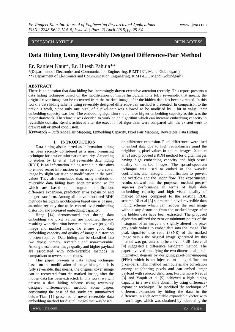
(a) Lee et al.’s method
(b) Its improvement
Figure 1: PPM for illustrating the data embedding
procedure [15]
We point out that, in an equivalent way, Lee et
al.’s [4] embedding procedure can be demonstrated
by a PPM shown in Fig. 1(a), in which a subset Z2 is
divided into two disjointed parts as black points and
blue points, each black point is mapped to a blue one
(indicated by a green arrow) and each blue point is
mapped to another blue point. Here, each point
Er. Ranjeet Kaur Int. Journal of Engineering Research and Applications www.ijera.com
ISSN : 2248-9622, Vol. 5, Issue 4, ( Part -2) April 2015, pp.25-34
www.ijera.com 27 | P a g e
represents the value of a pixel-pair and the black
points are used for expansion embedding while the
blue ones for shifting.
According to this PPM, for a cover pixel-pair (x,
y), its marked value can be determined in the
following way:
1) If y-x=0 (i.e., (x, y) is a red point), the marked
pixel-pair is taken as (x, y) itself.
2) If y-x =1 or y-x= -1 (i.e., (x, y) is a black point)
a) If the to-be-embedded data bit b=0, the marked
pixel-pair (x, y) is taken as itself.
b) If the to-be-embedded data bit b=1, the marked
pixel-pair (x, y) is taken as its associate blue point.
3) If y-x >1or y-x< -1 (i.e.,(x, y) is a blue point), the
marked pixel-pair is taken as its associate blue point.
The corresponding data extraction and image
restoration process can also be demonstrated
according to the PPM since it is an injection, i.e.,
each point has at most one inverse. The trivial
description is omitted. From the PPM viewpoint, Lee
et al.’s [4] difference-histogram based method is
actually implemented by modifying the two
dimensional pixel-intensity-histogram. Lee et al.’s [4]
method only modifies the second pixel of the pair.
Thus two modification directions, up and down, are
allowed in data embedding. This is to say, in PPM, a
point (x, y) can be either mapped to its upper
neighbour (x, y+1) or lower neighbour (x, y-1).
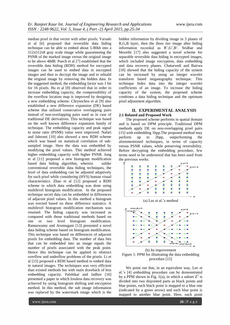
Actually, one can also modify the first pixel without
introducing additional distortion resulting in
modification directions left and right. In this way, the
associate mapped point of (x, y) has four choices: (x-
1, y), (x+1, y), (x, y+1) or (x, y-1) (see Fig. 2(a).
Based on these four modification directions, this
method can be improved by designing a new PPM
shown in Fig. 1(b). According to this figure, one can
see that more pixel-pairs (black points) are utilized
for expansion embedding, and the number of shifted
pixel-pairs (blue ones) is reduced as well. Here in
Fig. 1(b), the parameters k1 and k2 can be adaptively
selected by maximizing EC.
Figure 2: (a) By modifying either x or y by 1 has
four modification directions (b) The corresponding
difference-pair (d1, d2) also has four modification
directions, where d1=x-y, d2=y-z and z is a
prediction of y [15]
2.1.1 Embedding procedure: Modified DPM
For a pixel-pair, [15] proposes to compute two
difference values d1 =x-y and d2=y-z to form a two-
dimensional difference-histogram of (d1, d2) where z
is a prediction of y which will be clarified later.
Inspired by the aforementioned new PPM, we
will modify either x or y by 1 to 3. In this situation,
since it has four modification directions, the
difference-pair also has four modification directions,
or (see Fig. 2(b)). For example, by modifying y to
y+1,y+2 Or y+3, the modification direction to (x,y) is
“up” and the corresponding modification direction to
(d1,d2) is “upper-left”, since d1 changes to d1-1, d1-
2 and d1-3 and d2 changes to d2+1, d2+2 and d2+3.
Similarly by modifying x to x+1, x+2 Or x+3, the
modification direction to (x, y) is “right” and the
corresponding modification direction to (d1, d2) is
“right”, since d1 changes to d1+1, d1+2 and d1+3
and d2 changes to d2.Based on these modification
directions, we will introduce a new RDH scheme by
designing a DPM.
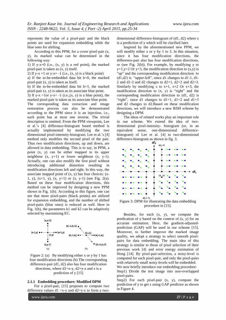
The ideas of related works play an important role
in our scheme. We extend the idea of two-
dimensional pixel-intensity- histogram (or, in an
equivalent sense, one-dimensional difference-
histogram) of Lee et al. [4] to two-dimensional
difference-histogram as shown in fig. 3.
Figure 3: DPM for illustrating the data embedding
procedure in [15].
Besides, for each (x, y), we compute the
predication of y based on the context of (x, y) for an
accurate estimation. Here, the gradient-adjusted-
prediction (GAP) will be used in our scheme [15].
Moreover, to further improve the marked image
quality, we adopt a strategy to select smooth pixel-
pairs for data embedding. The main idea of this
strategy is similar to those of pixel selection of their
previous work [4] and error energy estimation of
Hong [14]. By pixel-pair-selection, a noisy-level is
computed for each pixel-pair, and only the pixel-pairs
with relatively small noisy-levels will be embedded.
We now briefly introduce our embedding procedure:
Step1) Divide the test image into non-overlapped
pixel-pairs.
Step2) For each pixel-pair (x, y), compute the
prediction of y to get z using GAP predictor as shown
in Figure 4.

Er. Ranjeet Kaur Int. Journal of Engineering Research and Applications www.ijera.com
ISSN : 2248-9622, Vol. 5, Issue 4, ( Part -2) April 2015, pp.25-34
www.ijera.com 28 | P a g e
z =
v1 , if dv − dh > 80 v1 + u
2, if dv − dh ∈ 32, 80
v1 + 3u
4, if dv − dh ∈ 8, 32
u , if dv − dh ∈ −8, 8
v4 + 3u
4 , if dv − dh ∈ −32, −8
v4 + u
2 , if dv − dh ∈ −80, −32]
v4 , if dv − dh < −80
Figure 4: Gap predictor for calculating z [15]
Where v1 to v10 are neighbouring pixels taken from
surrounding window as described below in Figure 5.
Figure 5: Pixel window for calculation of z and
threshold t. [15]
Here i represent the row and j represents the column
co-ordinate of the test image
In this z has been rounded to its nearest integer by
using ceil function in Matlab.
Horizontal and vertical gradients dv and dh has been
calculated using formula below:
dv=|v3-v7|+|v4-v8|+|v1-v5|...........(2.1)
dh=|v3-v4|+|v1-v2|+|v4-v5|……...(2.2)
and u=(v1+v4)/2+(v3-v5)/4……...(2.3)
Step 3): Here, for discrete image, the noisy-level is
computed by summing both vertical and horizontal
differences of every two consecutive pixels in pixel
window, and it is less than or equal to 13*255.
Clearly a pixel-pair located in smooth regions may
have a small noisy-level.
Step 4): Finally, for each pixel-pair with noisy-level
less than a threshold T, compute the difference-pair
(d1, d2) and implement data embedding according to
the DPM defined below.
Table 1: Represents the data embedding procedure in x and y using difference pairs d1 and d2 and z predictor.
Conditions on d1
and d2
Operation in data
embedding
Modification direction to
pixel pair
Modification
direction
to(d1,d2)
Marked value
d1==0 & d2<=-2 Expansion
embedding
Down Lower-right (x, y-b)
d1==-1 & d2<=-2; Expansion
embedding
Left Left (x-b, y)
d1>=1 & d2<=-2 Shifting Down Lower-right (x, y-bmax)
d1<=-2 & d2<=-2 Shifting Left Left (x-bmax,y)
d1==0 & d2==-1 Expansion
embedding
Down Lower-right (x, y-b)
d1==-1 & d2==-1 Expansion
embedding
Left Left (x-b, y)
d1==1 & d2==-1 Expansion
embedding
Down Lower-right (x, y-b)
d1<=-2 & d2==-1 Shifting Left Left (x-bmax,y)
d1>=2 & d2==-1 Shifting Down Lower-right (x, y-bmax)
d1==0 & d2==0 Expansion
embedding
Up Upper-left (x,y+b)
d1>=1 & d2==0
Expansion
embedding
Down Lower-right (x, y-b)
d1>=2 & d2>=1 Shifting Right Right (x+bmax, y)
d1==1 & d2>=1 Expansion
embedding
Right Right (x+b, y)
d1==0 & d2>=1 Expansion
embedding
Up Upper-left (x,y+b)
d1<=-1 & d2>=0 Shifting Up Upper-left (x,y+bmax)
Er. Ranjeet Kaur Int. Journal of Engineering Research and Applications www.ijera.com
ISSN : 2248-9622, Vol. 5, Issue 4, ( Part -2) April 2015, pp.25-34
www.ijera.com 29 | P a g e
In order to achieve reversible data hiding,
some pixels are embedded and modified in order to
done embedding necessity and some pixels are
shifted by an exact value in order to make the
algorithm reversible. Table 1 gives all information
about the pixels which are embedded or shifted.
Step 5): All the modified pixel pairs are kept in a
matrix and corresponding record of embedded bits
has been done. In the end the watermarked image
has been saved to the folder along with the matrix
containing embedding bits.
2.1.2 Extraction Process
The following extraction procedure was
adopted during the experimental;
Step1) Load watermarked image in MATLAB
workspace. The difference between reversible and
non-reversible techniques is that reversible
techniques only need the watermarked image at
extraction process where as non-reversible
techniques need secret keys as well which is the
drawback of non-reversible techniques.
Step 2) Divide the whole image into non-
overlapped pixel pairs and start for extraction from
the pixels which are embedded in last in embedded
algorithm.
Step 3) compute the gap predictor variable z and
threshold t using the same gap predictor values
described in figure 4 and 5 in the embedded
algorithm.
Step 4) Evaluate modification direction variables
d1 and d2 using formula d1=x-y and d2=y-z where
x is first pixel of pixel pair and y is second pixel of
pixel pair.
Step 5) Apply the embedded extraction and shifting
according to the table listed below in Table 2.
Table 2: Table showing conditions on parameters
d1 and d2 in order to do extraction
Conditions on d1 and
d2
Extracted
data bit
Recovered
value
(d1==3 | d1==2) &
d2==-2
d1-1
(x,y+b)
(d1==3 | d1==2) &
d2<=-4
d1
(x,y+b)
(d1==0 | d1==1 ) &
d2<=-2
d1
(x,y+b)
d1>=4 & d2<=-5 None
(x,y+bmax)
d1<=-5 & d2<=-2 None (x+bmax,y)
(d1==1 & d2==-1) or
(d1==2 & d2==-2)
d1-1
(x,y+b)
(d1==3 & d2==-4) |
(d1==2 & d2==-3)|
(d1==1 & d2==-2)|
(d1==0 & d2==-1)
-1-d2
(x,y+b)
(d1==-4 | d1==-3 |
d1==-2 | d1==-1) &
-1-d1
(x+b,y)
d2==-1
(d1==4 & d2==-4) |
(d1==3 & d2==-3)|
(d1==2 & d2==-2)|
(d1==1 & d2==-1)
-1-d2
(x,y+b)
(d1==7 & d2==-2) |
(d1==8 & d2==-3)
-d2
(x,y+b)
d1<=-5 & d2==-1 None (x+bmax,y)
d1>=5 & d2==-4 None (x,y+bmax)
(d1<=0 & d1>=-3) &
(d2==0 | d2==1 |
d2==2 | d2==3)
-d1
(x,y-b)
(d1>=1) & (d2==0 |
d2==-1 | d2==-2 |
d2==-3)
-d2
(x,y+b)
d1>=5 & d2>=1 None (x-bmax,y)
(d1==1 | d1==2 |
d1==3 | d1==4) &
d2>=1
d1-1
(x-b,y)
(d1==0 | d1==-1 |
d1==-2 | d1==-3) &
d2>=1
-d1
(x,y-b)
d1<=-4 & d2>=3 None (x,y-bmax)
Step 6) Put the extracted bits in an array and
modified values of x and y in a matrix.
Step 7) Repeat the steps from step 3 and find the
extracted bits and modified pixels for all
overlapped pair by choosing the pairs in recursive
order to embedded process.
Step 8) Store the modified matrix of image and
extracted bit array in the folder and compare with
image taken in embedded process.
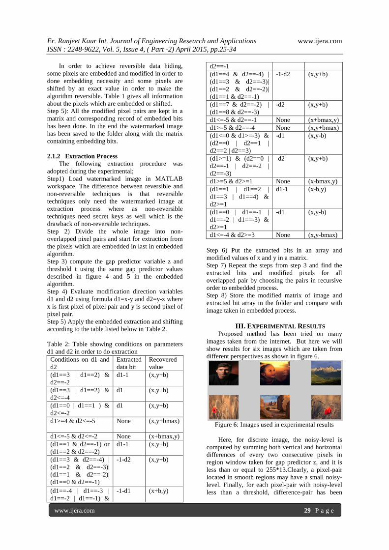
III. EXPERIMENTAL RESULTS Proposed method has been tried on many
images taken from the internet. But here we will
show results for six images which are taken from
different perspectives as shown in figure 6.
Figure 6: Images used in experimental results
Here, for discrete image, the noisy-level is
computed by summing both vertical and horizontal
differences of every two consecutive pixels in
region window taken for gap predictor z, and it is
less than or equal to 255*13.Clearly, a pixel-pair
located in smooth regions may have a small noisy-
level. Finally, for each pixel-pair with noisy-level
less than a threshold, difference-pair has been
Er. Ranjeet Kaur Int. Journal of Engineering Research and Applications www.ijera.com
ISSN : 2248-9622, Vol. 5, Issue 4, ( Part -2) April 2015, pp.25-34
www.ijera.com 30 | P a g e
computed and data embedding has been
implemented according to the DPM Table 1.
The criteria we adopted for choosing threshold are
different from Li et al [15]. We use formula for
obtaining maximum threshold which is the average
of all the noise levels in the image as illustrated
below.
Sum (Noise level)/ ((r*c)/2) …………………
(1)
where r and c are rows and columns in the image.
Threshold values are chosen by noisy-level
which is computed by summing both vertical and
horizontal differences of every two consecutive
pixels in gap generator window space V.
Results have been shown for threshold values
0, 5, 10, 15, 20 and tmax which is the average noise
level in the image.
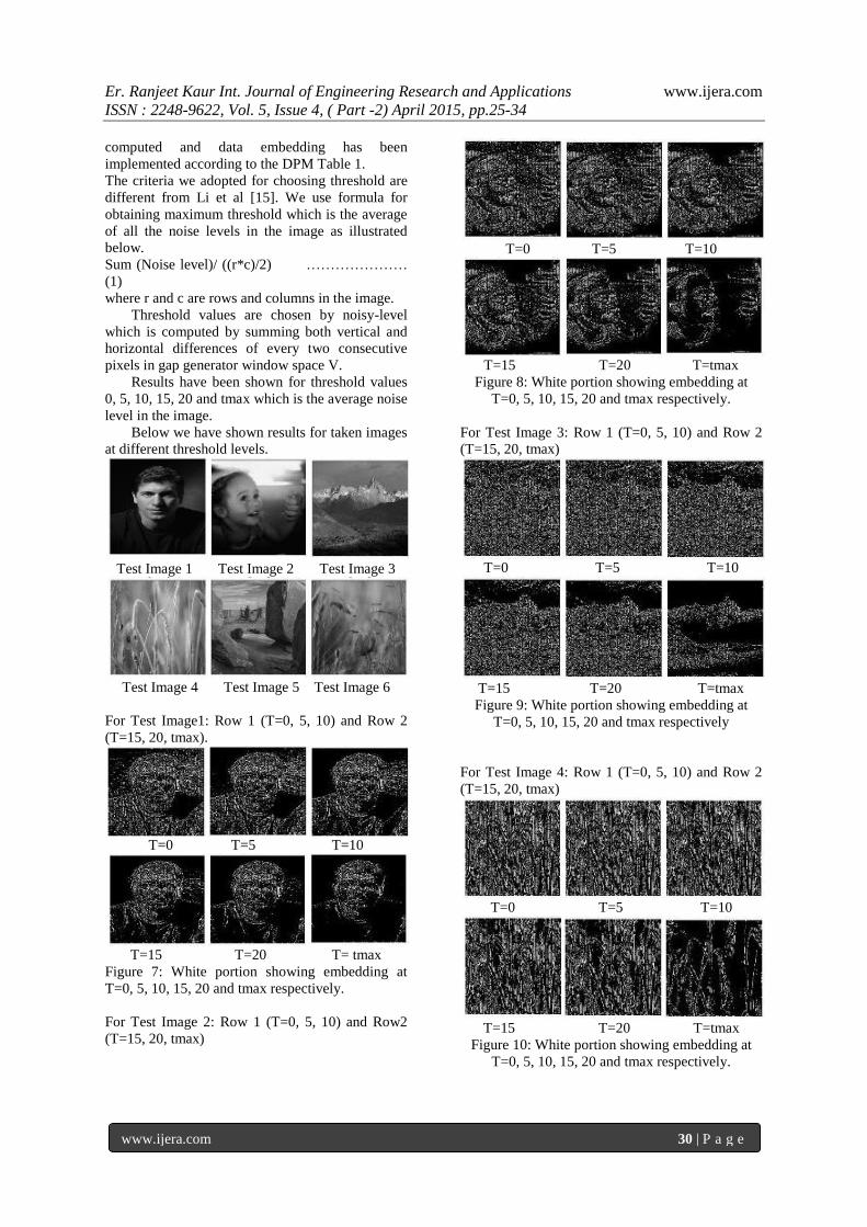
Below we have shown results for taken images
at different threshold levels.
Test Image 1 Test Image 2 Test Image 3
Test Image 4 Test Image 5 Test Image 6
For Test Image1: Row 1 (T=0, 5, 10) and Row 2
(T=15, 20, tmax).
T=0 T=5 T=10
T=15 T=20 T= tmax
Figure 7: White portion showing embedding at
T=0, 5, 10, 15, 20 and tmax respectively.
For Test Image 2: Row 1 (T=0, 5, 10) and Row2
(T=15, 20, tmax)
T=0 T=5 T=10
T=15 T=20 T=tmax
Figure 8: White portion showing embedding at
T=0, 5, 10, 15, 20 and tmax respectively.
For Test Image 3: Row 1 (T=0, 5, 10) and Row 2
(T=15, 20, tmax)
T=0 T=5 T=10
T=15 T=20 T=tmax
Figure 9: White portion showing embedding at
T=0, 5, 10, 15, 20 and tmax respectively
For Test Image 4: Row 1 (T=0, 5, 10) and Row 2
(T=15, 20, tmax)
T=0 T=5 T=10
T=15 T=20 T=tmax
Figure 10: White portion showing embedding at
T=0, 5, 10, 15, 20 and tmax respectively.
Er. Ranjeet Kaur Int. Journal of Engineering Research and Applications www.ijera.com
ISSN : 2248-9622, Vol. 5, Issue 4, ( Part -2) April 2015, pp.25-34
www.ijera.com 31 | P a g e
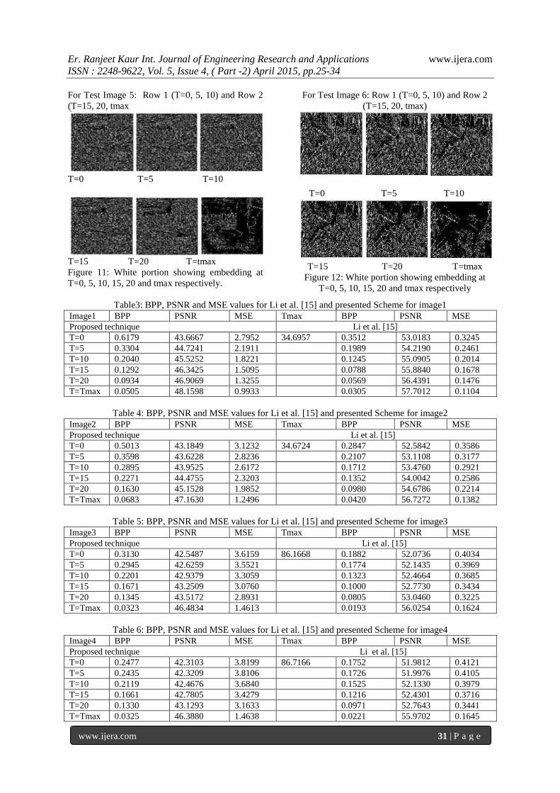
For Test Image 5: Row 1 (T=0, 5, 10) and Row 2
(T=15, 20, tmax
T=0 T=5 T=10
T=15 T=20 T=tmax
Figure 11: White portion showing embedding at
T=0, 5, 10, 15, 20 and tmax respectively.
For Test Image 6: Row 1 (T=0, 5, 10) and Row 2
(T=15, 20, tmax)
T=0 T=5 T=10
T=15 T=20 T=tmax
Figure 12: White portion showing embedding at
T=0, 5, 10, 15, 20 and tmax respectively
Table3: BPP, PSNR and MSE values for Li et al. [15] and presented Scheme for image1
Image1 BPP PSNR MSE Tmax BPP PSNR MSE
Proposed technique Li et al. [15]
T=0 0.6179 43.6667 2.7952 34.6957 0.3512 53.0183 0.3245
T=5 0.3304 44.7241 2.1911 0.1989 54.2190 0.2461
T=10 0.2040 45.5252 1.8221 0.1245 55.0905 0.2014
T=15 0.1292 46.3425 1.5095 0.0788 55.8840 0.1678
T=20 0.0934 46.9069 1.3255 0.0569 56.4391 0.1476
T=Tmax 0.0505 48.1598 0.9933 0.0305 57.7012 0.1104
Table 4: BPP, PSNR and MSE values for Li et al. [15] and presented Scheme for image2
Image2 BPP PSNR MSE Tmax BPP PSNR MSE
Proposed technique Li et al. [15]
T=0 0.5013 43.1849 3.1232 34.6724 0.2847 52.5842 0.3586
T=5 0.3598 43.6228 2.8236 0.2107 53.1108 0.3177
T=10 0.2895 43.9525 2.6172 0.1712 53.4760 0.2921
T=15 0.2271 44.4755 2.3203 0.1352 54.0042 0.2586
T=20 0.1630 45.1528 1.9852 0.0980 54.6786 0.2214
T=Tmax 0.0683 47.1630 1.2496 0.0420 56.7272 0.1382
Table 5: BPP, PSNR and MSE values for Li et al. [15] and presented Scheme for image3
Image3 BPP PSNR MSE Tmax BPP PSNR MSE
Proposed technique Li et al. [15]
T=0 0.3130 42.5487 3.6159 86.1668 0.1882 52.0736 0.4034
T=5 0.2945 42.6259 3.5521 0.1774 52.1435 0.3969
T=10 0.2201 42.9379 3.3059 0.1323 52.4664 0.3685
T=15 0.1671 43.2509 3.0760 0.1000 52.7730 0.3434
T=20 0.1345 43.5172 2.8931 0.0805 53.0460 0.3225
T=Tmax 0.0323 46.4834 1.4613 0.0193 56.0254 0.1624
Table 6: BPP, PSNR and MSE values for Li et al. [15] and presented Scheme for image4
Image4 BPP PSNR MSE Tmax BPP PSNR MSE
Proposed technique Li et al. [15]
T=0 0.2477 42.3103 3.8199 86.7166 0.1752 51.9812 0.4121
T=5 0.2435 42.3209 3.8106 0.1726 51.9976 0.4105
T=10 0.2119 42.4676 3.6840 0.1525 52.1330 0.3979
T=15 0.1661 42.7805 3.4279 0.1216 52.4301 0.3716
T=20 0.1330 43.1293 3.1633 0.0971 52.7643 0.3441
T=Tmax 0.0325 46.3880 1.4638 0.0221 55.9702 0.1645
Er. Ranjeet Kaur Int. Journal of Engineering Research and Applications www.ijera.com
ISSN : 2248-9622, Vol. 5, Issue 4, ( Part -2) April 2015, pp.25-34
www.ijera.com 32 | P a g e
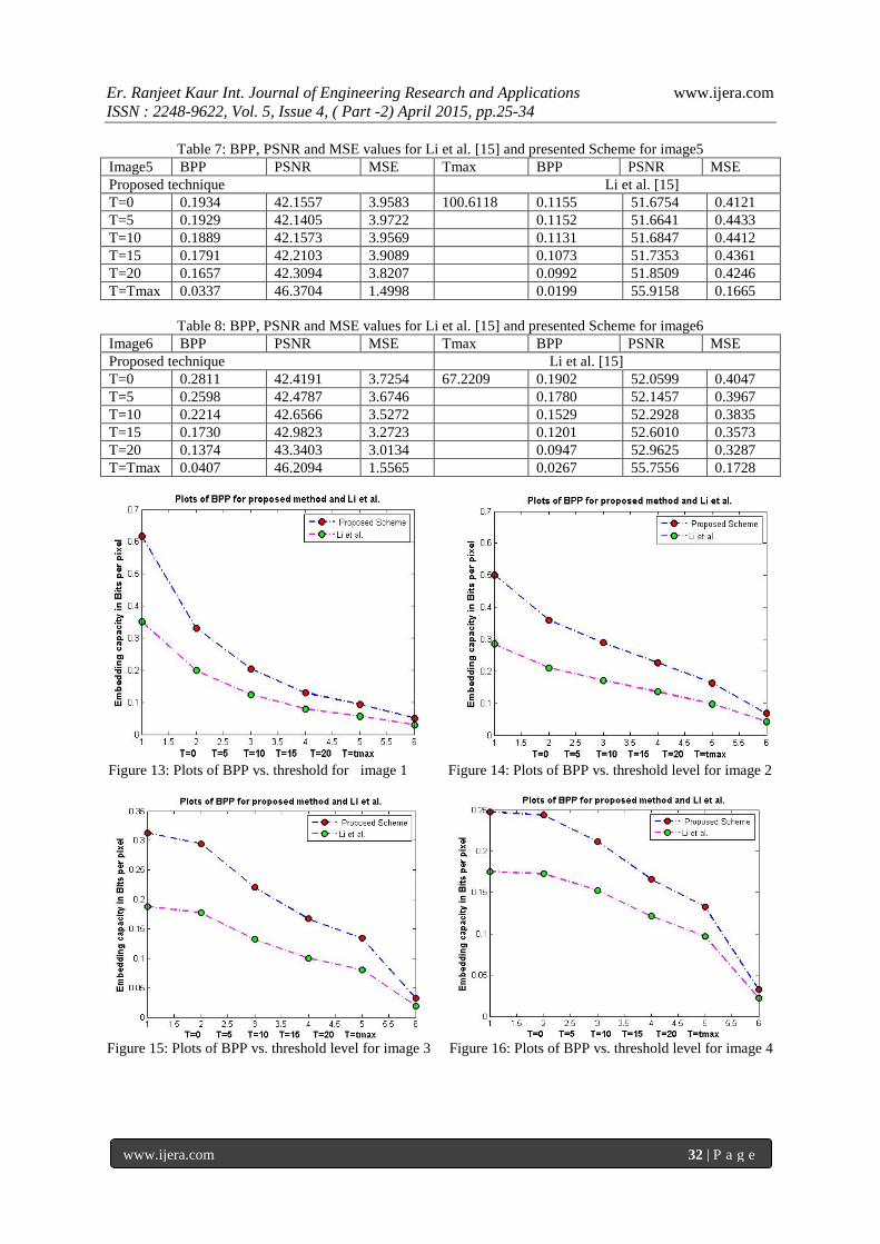
Table 7: BPP, PSNR and MSE values for Li et al. [15] and presented Scheme for image5
Image5 BPP PSNR MSE Tmax BPP PSNR MSE
Proposed technique Li et al. [15]
T=0 0.1934 42.1557 3.9583 100.6118 0.1155 51.6754 0.4121
T=5 0.1929 42.1405 3.9722 0.1152 51.6641 0.4433
T=10 0.1889 42.1573 3.9569 0.1131 51.6847 0.4412
T=15 0.1791 42.2103 3.9089 0.1073 51.7353 0.4361
T=20 0.1657 42.3094 3.8207 0.0992 51.8509 0.4246
T=Tmax 0.0337 46.3704 1.4998 0.0199 55.9158 0.1665
Table 8: BPP, PSNR and MSE values for Li et al. [15] and presented Scheme for image6
Image6 BPP PSNR MSE Tmax BPP PSNR MSE
Proposed technique Li et al. [15]
T=0 0.2811 42.4191 3.7254 67.2209 0.1902 52.0599 0.4047
T=5 0.2598 42.4787 3.6746 0.1780 52.1457 0.3967
T=10 0.2214 42.6566 3.5272 0.1529 52.2928 0.3835
T=15 0.1730 42.9823 3.2723 0.1201 52.6010 0.3573
T=20 0.1374 43.3403 3.0134 0.0947 52.9625 0.3287
T=Tmax 0.0407 46.2094 1.5565 0.0267 55.7556 0.1728
Figure 13: Plots of BPP vs. threshold for image 1 Figure 14: Plots of BPP vs. threshold level for image 2
Figure 15: Plots of BPP vs. threshold level for image 3 Figure 16: Plots of BPP vs. threshold level for image 4
Er. Ranjeet Kaur Int. Journal of Engineering Research and Applications www.ijera.com
ISSN : 2248-9622, Vol. 5, Issue 4, ( Part -2) April 2015, pp.25-34
www.ijera.com 33 | P a g e
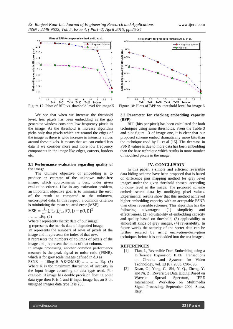
Figure 17: Plots of BPP vs. threshold level for image 5 Figure 18: Plots of BPP vs. threshold level for image 6
We see that when we increase the threshold
level, less pixels has been embedding as the gap
generator window considers low frequency pixels in
the image. As the threshold is increase algorithm
picks only that pixels which are around the edges of
the image as there is wide increase in intensity values
around these pixels. It means that we can embed less
data if we consider more and more low frequency
components in the image like edges, corners, borders
etc.
3.1 Performance evaluation regarding quality of
the image
The ultimate objective of embedding is to
produce an estimate of the unknown noise-free
image, which approximates it best, under given
evaluation criteria. Like in any estimation problem,
an important objective goal is to minimize the error
of the result as compared to the unknown,
uncorrupted data. In this respect, a common criterion
is minimizing the mean squared error (MSE)
MSE =1
mn [f i, j − g(i, j)]2n
j=1mi=1 .
……….Eq. (2)
Where f represents matrix data of our image,
g represents the matrix data of degraded image,
m represents the numbers of rows of pixels of the
image and i represents the index of that row.
n represents the numbers of columns of pixels of the
image and j represent the index of that column.
In image processing, another common performance
measure is the peak signal to noise ratio (PSNR),
which is for grey scale images defined in dB as
PSNR = 10log10 *(R^2/MSE)………….. Eq. (3)
Where R is the maximum fluctuation of intensity in
the input image according to data type used. For
example, if image has double precision floating point
data type then R is 1 and if input image has an 8 bit
unsigned integer data type R is 255.
3.2 Parameter for checking embedding capacity
(BPP)
BPP (bits per pixel) has been calculated for both
techniques using same thresholds. From the Table 3
and plot figure 13 of image one, it is clear that our
proposed scheme embed dramatically more bits than
the technique used by Li et al [15]. The decrease in
PSNR values is due to more data has been embedding
than the base technique which results in more number
of modified pixels in the image.
IV. CONCLUSION In this paper, a simple and efficient reversible
data hiding scheme have been proposed that is based
on difference pair mapping method for gray level
images under the given threshold chosen according
to noisy level in the image. The proposed scheme
embeds secret data by modifying pixel values.
Experimental results show that this method achieved
higher embedding capacity with an acceptable PSNR
than other reversible schemes. This algorithm has the
following advantages: (1) simplicity and
effectiveness, (2) adjustability of embedding capacity
and quality based on threshold, (3) applicability to
almost all kinds of grey images, (4) reversibility. In
future works the security of the secret data can be
further secured by using encryption-decryption
techniques before it is embedded into the test images.
REFERENCES [1] Tian, J., Reversible Data Embedding using a
Difference Expansion, IEEE Transactions
on Circuits and Systems for Video
Technology, vol. 13 (8), 2003, 890-896.
[2] Xuan, G., Yang, C., Shi, Y. Q., Zheng, Y.
and Ni, Z., Reversible Data Hiding Based on
Wavelet Spread Spectrum, IEEE
International Workshop on Multimedia
Signal Processing, September 2004, Siena,
Italy.
Er. Ranjeet Kaur Int. Journal of Engineering Research and Applications www.ijera.com
ISSN : 2248-9622, Vol. 5, Issue 4, ( Part -2) April 2015, pp.25-34
www.ijera.com 34 | P a g e
[3] Ni, Z., Shi, Y. Q., Ansari, N. and Su, W.,
Reversible Data Hiding, IEEE Transactions
On Circuits and Systems for Video
Technology, vol. 16(3), 2006, 354-362.
[4] Lee, S. K., Suh, Y. H. and Ho, Y. S.,
Reversible Image Authentication Based on
Watermarking, in Proc. IEEE ICME, 2006,
1321-1324.
[5] Yaqub, M. K. and Jaber, A. A., Reversible
Watermarking using Modified Difference
Expansion, International Journal of
Computing & Information Sciences”, vol.
4(3), 2006, 134-142.
[6] Varsaki, E., Fotopoulos, V. and Skodras, A.
N., A Reversible Data Hiding Technique
Embedding in the Histogram, Hellenic Open
University: Technical Report HOU-CS-TR-
2006-08-GR, 2008.
[7] Puech, W., Chaumont, M. and Strauss, O., A
Reversible Data Hiding Method for
Encrypted Images, Author manuscript-
Security, Forensics, Steganography, and
Watermarking of Multimedia Contents,
IS&T/SPIE Electronic Imaging, 1-3 July
2008, San Jose, United States.
[8] Hu, Y., Lee, H. K. and Li, J., DE-Based
Reversible Data Hiding with Improved
Overflow Location Map, IEEE Transactions
On Circuits and Systems For Video
Technology, vol. 19 (2), 2009, 250-260.
[9] Chrysochos, E., Varsaki, E. E., Fotopoulos,
V. and Skodras, A. N., High Capacity
Reversible Data Hiding using Overlapping
Difference Expansion, 10th International
workshop on Image Analysis, 6-8 May
2009. London, UK.
[10] Nafari, M. and Jahromi, N. M., Reversible
Data Hiding Based on Statistical Correlation
of Blocked Sub-sampled Image,
International Journal on New Computer
Architectures and their Applications
(IJNCAA), vol. 1 (1), 2011, 52-60.
[11] Jung, S. W., Ha, L. T. and Ko, S. J., A New
Histogram Modification Based Reversible
Data Hiding Algorithm Considering the
Human Visual System, IEEE Signal
Processing Letters, vol. 18, (2), 2011, 95-98.
[12] Zhao, Z., Luo, H., Lu, Z. M. and Pan, J. S.,
Reversible Data Hiding Based on Multilevel
Histogram Modification and Sequential
Recovery, International Journal of
Electronics and Communications (AEU),
vol. 65, 2011, 814-826.
[13] Ramaswamy, R. and Arumugam, V.,
Lossless Data Hiding Based on Histogram
Modification, International Arab Journal of
Information Technology, vol. 9(5), 2012,
445-451.
[14] Hong, W., Adaptive Reversible Data Hiding
Method Based on Error Energy Control and
Histogram Shifting, Optics
Communications, vol. 285(2), 2012, 101-
108.
[15] Li, X., Zhang, W., Gui, X. and Yang, B., A
Novel Reversible Data Hiding Scheme
Based on 2-Dimensional Difference-
Histogram Modification, IEEE Transactions
on Information Forensics And Security, vol.
8(7), 2013, 1091-1099.
[16] Palshikar, N. and Jadhav, S.,Lossless Data
Hiding using Histogram Modification and
Hash Encryption Scheme, International
Journal of Emerging Technology and
Advanced Engineering, vol. 3(1), 2014, 485-
493.
[17] Sridhar. N. J. and Moorthi, K., Reversible
Watermarking on Encryption Image
Classification and Dynamic Colour
Techniques, International Journal of
Innovative Research in Science, Engineering
and Technology, vol. 3(1), 2014, 182-187.
[18] Chaturvedi, P. and Bairwa, R. K., An
Integer Wavelet Transform Based
Steganography Technique for Concealing
Data in Coloured Images, International
Journal of Recent Research and Review, vol.
7(2), 2014, 49-57.