data locality in mapreduce: a network perspectivewwang136/index_files/mapreduce... · data locality...
TRANSCRIPT

Data Locality in MapReduce: A Network Perspective
Weina Wanga,∗, Lei Yinga
aSchool of Electrical, Computer and Energy Engineering, Arizona State UniversityTempe, AZ 85281, USA
Abstract
Data locality, a critical consideration for the performance of task scheduling inMapReduce, has been addressed in the literature by increasing the number oflocally processed tasks. In this paper, we view the data locality problem from anetwork perspective. The key observation is that if we make appropriate use ofthe network to route the data chunk to the machine where it will be processedin advance, then processing a remote task is the same as processing a localtask. However, to benefit from such a strategy, we must (i) balance the tasksassigned to local machines and those assigned to remote machines, and (ii) de-sign the routing algorithm to avoid network congestion. Taking these challengesinto consideration, we propose a scheduling/routing algorithm, named the JointScheduler, which utilizes both the computing resources and the communicationnetwork efficiently. We prove that the Joint Scheduler is throughput optimal;i.e., it supports any load that is supportable by any other algorithm. Simulationresults demonstrate that with popularity skew, the Joint Scheduler improves thethroughput and delay performance significantly compared to the Hadoop FairScheduler with delay scheduling, which is the de facto industry standard.
Keywords: MapReduce, Data locality, Scheduling, Routing, Throughput
1. Introduction
The MapReduce framework [1] has been widely deployed in large computingclusters for the growing need of big data analysis. Hadoop is one of the mostpopular implementations of the MapReduce framework and has been adoptedby various organizations.
The MapReduce framework is implemented on top of distributed file systemssuch as the Google File System (GFS) and the Hadoop Distributed File System(HDFS) [2], which divide large datasets into data chunks and store multiplereplicas of each chunk on different machines. MapReduce jobs are submitted torequest data processing and each job is divided into a number of map tasks andreduce tasks. A map task reads one data chunk and processes it to generate
∗Corresponding author, phone number: +1 515-509-5697.Email addresses: [email protected] (Weina Wang), [email protected] (Lei Ying)
Preprint submitted to Elsevier December 4, 2015

intermediate results. Reduce tasks fetch these intermediate results and conductfurther computations to get the final results.
Map tasks and reduce tasks are assigned to machines according to a schedul-ing algorithm. During task scheduling, an important consideration is to placecomputation near data, i.e., to assign a task on or close to the machine thatstores its input data on local disks. This is commonly referred to as the data lo-cality problem. The data locality problem is particularly crucial for map taskssince they read data from the distributed file system and map functions aredata-parallel. Besides, according to an empirical trace study from a productionMapReduce cluster [3], the majority of jobs are map-intensive, and many ofthem are map-only. Therefore we focus on data locality in map task schedul-ing algorithms and assume that reduce tasks are not the bottleneck of the jobprocessing or the communication network.
We call a machine a local machine for a map task if it has the input datachunk of this task on its local disks, and we call this map task a local task on thismachine; otherwise, the machine is called a remote machine for this map taskand this map task is called a remote task on the machine. We also use the termlocality to refer to the fraction of tasks that are executed on local machines.In most of the existing work, launching a map task on a remote machine isconsidered to be inefficient, since a remote machine needs to first retrieve theinput data from other machines through the communication network beforeprocessing it, which introduces an additional delay to the task execution. Solocal and remote tasks are often modeled with different processing times.
This view of data locality in MapReduce is arguable. If the communicationnetwork that connects the machines had infinite capacity and could transfer datainstantaneously, then there would be no difference between assigning a task toits local machines or to other machines. Thus the time of processing a remotetask depends on the capacity of the communication network and the schedulingalgorithm that allocates tasks. If data can be routed in advance so that machinesdo not spend time on waiting for input data before executing tasks, then eventhough the network capacity is finite, we can still achieve the same throughputas if all tasks are local. Inspired by this intuition, we study the data localityproblem from a network perspective beyond just abstracting the effect of thecommunication network as a “longer processing time”. We adopt an approachthat explicitly takes account of the structure of the communication networkand quantify fundamental limits on the capacity of a MapReduce cluster withnetwork constraints. Then we explore joint scheduling and routing algorithmsto fully exploit the system capacity.
To optimize the performance, we face the following challenges: how to strikethe right balance between local and remote tasks, and how to route the traffic inthe network appropriately to avoid congestion. Failure to meet these challengesmay result in slow data transmission and a waste of computing resources andmay even harm the throughput performance. These challenges are more pro-nounced when data are not ideally uniformly distributed across the cluster [4],in which case placing all the computation near data results in heavy load onsome machines while leaving other machines lightly utilized or idle.
2

In this paper, we first quantify fundamental limits on the capacity of aMapReduce cluster with network constraints by characterizing its capacity re-gion, which consists of arrival rate vectors of tasks for which there exists ascheduling/routing algorithm that stabilizes the system. Then we propose aqueueing architecture that enables us to jointly design the scheduling and rout-ing algorithm with the above challenges taken into consideration to achievethroughput optimality, i.e., to stabilize the system for any arrival rate vectorstrictly within the capacity region. We call our scheduling/routing algorithmthe Joint Scheduler. Our contributions are summarized as follows.
• We advocate studying the data locality problem from a network perspective.We propose to route the input data of tasks in advance through the commu-nication network. Joint task scheduling and routing, taking communicationnetwork constraints into consideration, should be designed to fully exploitthe system capacity.
• We propose a queueing architecture that captures both the data transmis-sion in the communication network and the task execution by machines.This queueing architecture makes accurate status information of the net-work traffic and the workload of machines available, and thus enables jointscheduling and routing according to the information.
• Based on the proposed queueing architecture, we develop a task scheduling/routing algorithm, named the Joint Scheduler, that uses join the shortestqueue policy (with blocking under some conditions) to assign incoming tasksto machines and route tasks in the communication network.
• We characterize the capacity region of a MapReduce cluster with data local-ity and communication network constraints. Then we prove that the JointScheduler is throughput optimal; i.e., it stabilizes the system for any ar-rival rate vector strictly within the capacity region. Therefore, the JointScheduler utilizes the computing resources efficiently by balancing the tasksassigned to local machines and those assigned to remote machines, and ex-ploits the communication network capacity by balancing the traffic load toavoid congestion.
Note that although the Joint Scheduler is in spirit similar to a MaxWeight/backpressure algorithm [5], the coupling between a task and its input datasets the scheduling/routing problem in a MapReduce cluster apart from atraditional network scheduling problem, in which a packet that arrives at aservice node becomes ready for the service immediately.
The rest of this paper is organized as follows. Section 2 discusses the relatedwork in literature. Section 3 introduces the system model. Section 4 presentsthe design of our Joint Scheduler and Section 5 establishes the throughput opti-mality. Simulation results are given in Section 6 to compare the Joint Schedulerand the Hadoop Fair Scheduler. The paper is concluded in Section 7.
3
... ...
... rack switches
cluster switch
machines
...
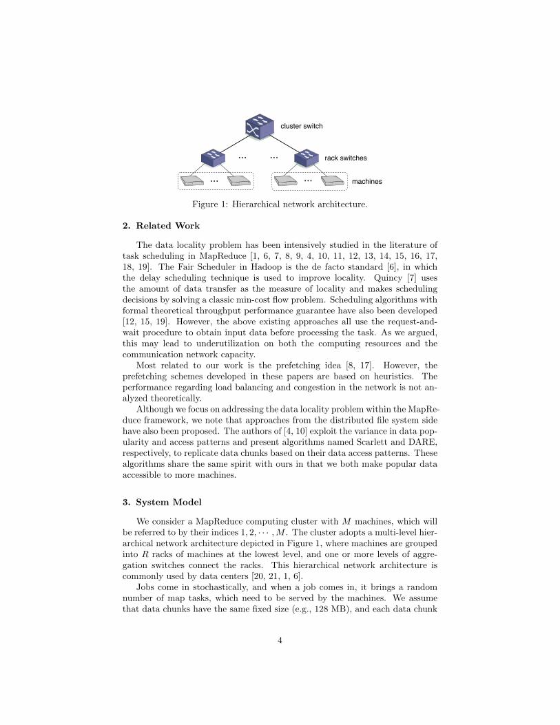
Figure 1: Hierarchical network architecture.
2. Related Work
The data locality problem has been intensively studied in the literature oftask scheduling in MapReduce [1, 6, 7, 8, 9, 4, 10, 11, 12, 13, 14, 15, 16, 17,18, 19]. The Fair Scheduler in Hadoop is the de facto standard [6], in whichthe delay scheduling technique is used to improve locality. Quincy [7] usesthe amount of data transfer as the measure of locality and makes schedulingdecisions by solving a classic min-cost flow problem. Scheduling algorithms withformal theoretical throughput performance guarantee have also been developed[12, 15, 19]. However, the above existing approaches all use the request-and-wait procedure to obtain input data before processing the task. As we argued,this may lead to underutilization on both the computing resources and thecommunication network capacity.
Most related to our work is the prefetching idea [8, 17]. However, theprefetching schemes developed in these papers are based on heuristics. Theperformance regarding load balancing and congestion in the network is not an-alyzed theoretically.
Although we focus on addressing the data locality problem within the MapRe-duce framework, we note that approaches from the distributed file system sidehave also been proposed. The authors of [4, 10] exploit the variance in data pop-ularity and access patterns and present algorithms named Scarlett and DARE,respectively, to replicate data chunks based on their data access patterns. Thesealgorithms share the same spirit with ours in that we both make popular dataaccessible to more machines.
3. System Model
We consider a MapReduce computing cluster with M machines, which willbe referred to by their indices 1, 2, · · · ,M . The cluster adopts a multi-level hier-archical network architecture depicted in Figure 1, where machines are groupedinto R racks of machines at the lowest level, and one or more levels of aggre-gation switches connect the racks. This hierarchical network architecture iscommonly used by data centers [20, 21, 1, 6].
Jobs come in stochastically, and when a job comes in, it brings a randomnumber of map tasks, which need to be served by the machines. We assumethat data chunks have the same fixed size (e.g., 128 MB), and each data chunk
4
is replicated and placed at three different machines, which is the default config-uration of HDFS. Therefore, each task is associated with three local machines.When a task is launched on a remote machine, the machine cannot start pro-cessing the task until the necessary data arrives. According to the associatedlocal machines, tasks can be classified into types denoted by
~L = (m1~L,m2
~L,m3
~L),
where mi~L, i = 1, 2, 3 are the indices of the three local machines, in increasing
order. For example, if the data chunk associated with a task is stored at ma-chines 1, 21 and 23 then ~L = (1, 21, 23). We assume machine m1
~Lis in rack r1
~L,
and machine m2~L
and m3~L
are in the same rack r2~L
according to Hadoop’s data
replication policy [2].
3.1. Arrivals and Service
We consider a time-slotted system. Let A~L(t) denote the number of type ~Ltasks arriving at the beginning of time slot t. We assume that {A~L(t), t ≥ 0}is an i.i.d. sequence with arrival rate E[A~L(t)] = λ~L and the second momentE[(A~L(t))2] is finite. We assume that there is a positive probability that thereis no arrival at a time slot.
Let λ = (λ~L : ~L ∈ L) be the arrival rate vector, where L is the set of task
types with arrival rates greater than zero; i.e., L = {~L : λ~L > 0}.The service/processing time of each task is assumed to follow a geometric
distribution with parameter ϕ, where 0 < ϕ < 1.The following notation is used throughout this paper:
- Mr: the set of machines in rack r.
- rm: the index of the rack that machine m is in.
- For each task type ~L, the set of local machines is denoted by
M~L = {m1~L,m2
~L,m3
~L}.
- For each machine m, the set of types such that tasks of these types arelocal on machine m is denoted by
Lm = {~L ∈ L : m ∈M~L}.
3.2. Network Queueing Model
In the considered hierarchical network architecture, a set of machines aremounted within a rack and interconnected by a rack switch. These rack switcheshave a number of uplink connections to the cluster switch, which can use 1-Gbpsor 10-Gbps links. For economic considerations, the design of the network con-nections usually introduces oversubscription since all the interrack traffic needsto go through the cluster switch. For example, in the network that 40 serversin the same rack connect to the rack switch by 1-Gbps ports, rack switches may
5
machines
......
...
rack switches
cluster switch
task arrivals ...
...
rack incoming queues
rack outgoingqueue
machine incomingqueues
machine outgoing queue
processingqueue
Qm,2
�m,2
Qm,0 Qm,1
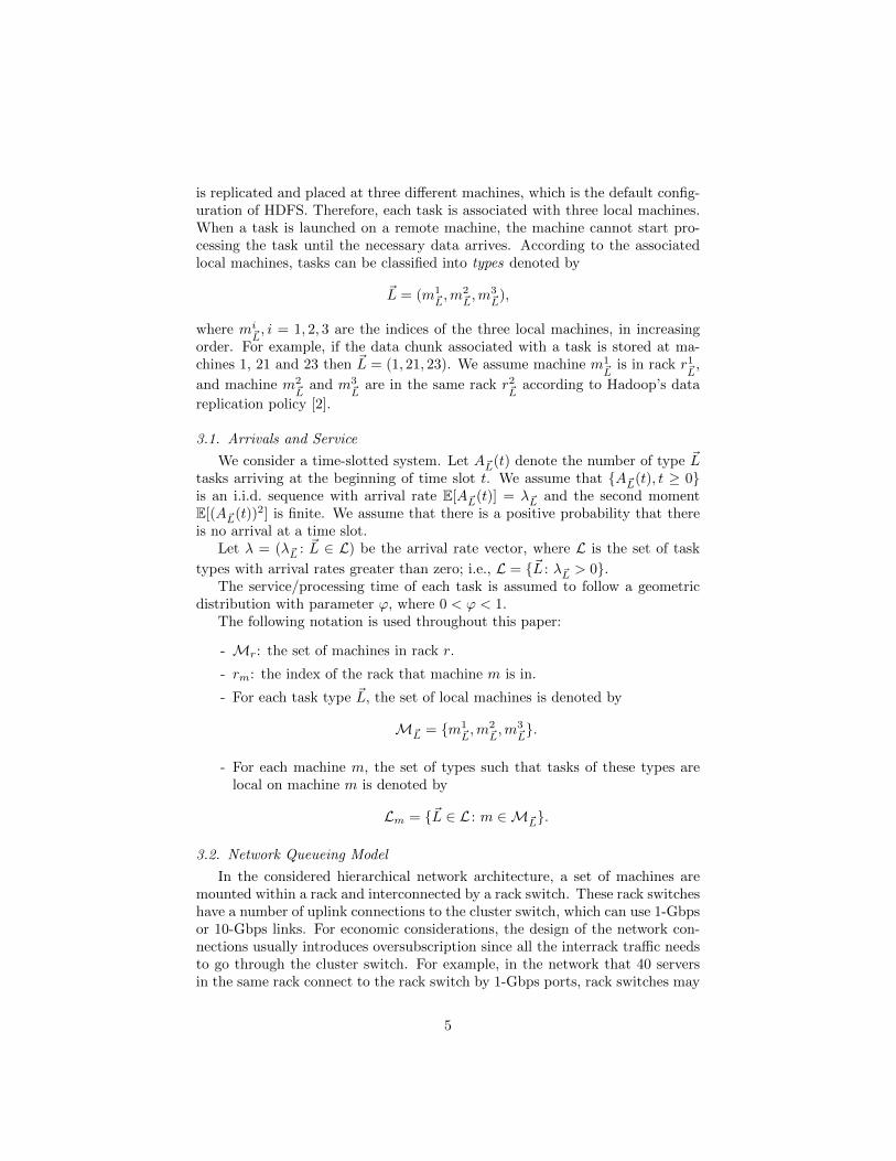
Figure 2: Network queueing model.
have between four and eight 1-Gbps uplinks to the cluster switch, correspond-ing to an oversubscription factor between 5 and 10 for communication acrossracks [21]. Therefore the cluster-level bandwidth resource is relatively scarcecompared with the rack-level.
Data transmission in the network consumes bandwidth. Since each machineconnects to the network through the rack switch, the bandwidth between themachine and the rack switch constrains the incoming and outgoing data trans-mission rates of the machine. When there is a large amount of data that needsto be sent or received by a machine, the unfinished data will be backlogged atsome queues. Let this constraint on the incoming and outgoing data transmis-sion rates of each machine be B1 data chunks per time slot. For the interracktraffic, due to oversubscription, the machines in one rack cannot communicatewith machines in other racks at their full bandwidth simultaneously. There areconstraints on the overall incoming and outgoing data transmission rates of therack. Let this constraint be B2 data chunks per time slot. This rack bandwidthis shared by machines in the same rack.
Based on the network hierarchy, the communication network in the clusteris modeled as depicted in Figure 2. For each machine m, Qm,1 and Qm,2 are thequeues for the outgoing traffic and incoming traffic of the machine, respectively.Therefore, at most B1 data chunks depart from each queue during one time slot.Similarly, for each rack r, Xr,1 and Xr,2 are the queues for the outgoing trafficand incoming traffic of the rack, respectively, and at most B2 data chunks departfrom each queue during one time slot. We call Qm,1 and Qm,2 the machineoutgoing queue and the machine incoming queue, and we call Xr,1 and Xr,2 therack outgoing queue and the rack incoming queue. The queue Qm,0 and otherlabels will be introduced in Section 4.1 and Section 5.2, respectively. Machine mcommunicates with machine a in the same rack through the path (Qm,1, Qa,2).An example is shown in Figure 2 for m = 1, a = 2 with corresponding path(Q1,1, Q2,2). Machine m communicates with machine b in another rack through
6

the path (Qm,1, Xrm,1, Xrb,2, Qb,2), as shown in Figure 2 for m = 1, b = 20with path (Q1,1, X1,1, Xr,2, Q20,2). Since each map task is associated with adata chunk and the network is used to transfer the data chunks to be processedremotely, B1 and B2 can also be viewed as number of tasks per time slot. Thephrases transmitting tasks and transmitting data are used interchangeably inthe context of communication. The lengths of the queues are counted as thenumber of tasks that have input data chunks in the queues.
Remark 1. We assume without loss of generality that B1 is larger than orequal to 1 since otherwise we can rescale the duration of the time slot. The rackswitches usually use 1-Gbps uplinks. This transmission rate is usually largerthan the data processing rate performed by map functions. So we assume aservice rate ϕ smaller than 1 after rescaling. The rate B2 is larger than B1 andsmaller than R ·B1 due to oversubscription.
4. Map Task Scheduling/Routing
In this section, we present a new algorithm that performs task schedulingand routing jointly. We call this scheduler the Joint Scheduler, which is alsoreferred to as JS in this paper. This algorithm includes two parts: the firstpart assigns incoming tasks to some machines to serve or to the communicationnetwork to transmit as tasks arrive at the cluster; the second part routes thetasks in the communication network.
Before we describe our algorithm in detail, we first further elaborate on ourqueueing architecture of the cluster. We have derived the queueing model ofthe communication network in Section 3.2. Now we introduce the architectureof the processing queues in JS. For each machine m, the scheduler maintainsa processing queue Qm,0 to buffer the tasks assigned to machine m for localprocessing and the tasks whose data have been transferred to machine m forremote processing. Therefore, the tasks in Qm,0 all have the corresponding dataon machine m, and thus are ready for the processing.
4.1. Task Scheduling/Routing Algorithm
As discussed in the introduction, the low efficiency of remote task processingcan be ascribed to the underutilization of machines while waiting for input data.Our algorithm addresses data locality by intelligently routing data in advance,which reduces the idling time of machines without causing network congestion.
For each queue Q in the communication network, the set of queues that canreceive data directly from Q is called the set of candidate destinations of Q andis denoted by D(Q). These sets represent the connectivity of the system, whichis illustrated in Figure 2. We describe this candidate destination set for eachqueue as follows.
• For each machine m, the machine outgoing queue Qm,1 can send data to therack outgoing queue and to the machine incoming queues in the same rack,so
D(Qm,1) = {Xrm,1} ∪ {Qm′,2 | m′ ∈Mrm}.
7
Algorithm 1 The Joint Scheduler
at time slot t
for task in incoming tasks dofind the task type ~Lassign the task to the shortest queue in Q~L
for Q in the communication network dofind the shortest queue Dt
Q in D(Q)
if DtQ(t) < Q(t) then
send data to DtQ
elseblock the outgoing traffic from Q
• The machine incoming queue Qm,2 can only send data to the processingqueue Qm,0, so
D(Qm,2) = {Qm,0}.
• For each rack r, the rack outgoing queue Xr,1 can send data to the rackincoming queues of all the racks, so
D(Xr,1) = {Xr′,2 | r′ = 1, · · · , R}.
• The rack incoming queue Xr,2 can send data to the machine incoming queuesin its own rack, so
D(Xr,2) = {Qm,2 | m ∈ Rr}.
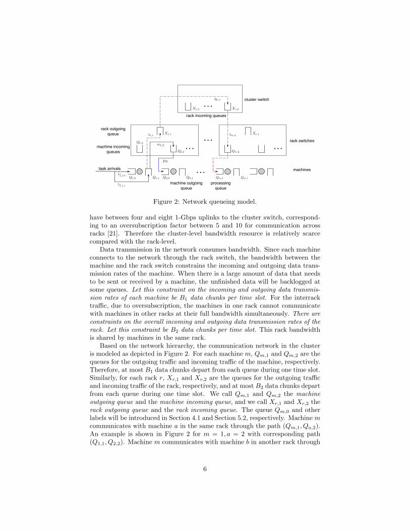
Now we present the Joint Scheduler as follows. The pseudocode is shown inAlgorithm 1 and a toy example illustrating the procedure of the algorithm isshown after.
• Task Assignment for New Tasks. When a type ~L task comes in, thescheduler assigns it to the shortest queue inQ~L = {Qm,i | m ∈M~L, i = 0, 1}.Note that if a task is assigned to Qm,0, it means that the task will beprocessed at local machine m; if it is assigned to Qm,1, it means machinem needs to transmit the data chunk associated with the task to another(remote) machine to process.
• Routing in the Communication Network. For each queue in the com-munication network, we use a join the shortest queue algorithm with blockingto route tasks: each queue Q in the communication network first finds theshortest queue in the candidate destination set D(Q), denoted by Dt
Q; then
it compares the queue length DtQ(t) with Q(t). If Dt
Q(t) < Q(t), Q sends
data to DtQ; otherwise Q does not send any data. If Q is the machine incom-
ing queue or machine outgoing queue, then by the bandwidth constraint itcan send at most B1 data chunks during each time slot; similarly, if Q is therack incoming queue or rack outgoing queue, then it can send at most B2
data chunks during each time slot according to the bandwidth constraint.
8

Q1,0(t) = 4
Q1,1(t) = 3
Q2,0(t) = 2
Q2,1(t) = 1 Q3,1(t) = 2
Q3,0(t) = 2
Q1,2(t) = 3 Q2,2(t) = 4
X1,1(t) = 2
rack switches
machines
a task of type (1, 2, 3) arrives
Figure 3: A toy example illustrating the Joint Scheduler.
A Toy Example. We use a toy example shown in Figure 3 to illustrate theprocedure of the Joint Scheduler. For the first step, a task of type ~L = (1, 2, 3)arrives at the system. The scheduler assigns it to Q2,1, which is the shortestqueue in Q(1,2,3) = {Q1,0, Q1,1, Q2,0, Q2,1, Q3,0, Q3,1}. For the second step, weuse Q1,1 and Q2,1 to explain. The candidate destination set of Q1,1 is
D(Q1,1) = {Q1,2, Q2,2, X1,1}.
At time slot t, the shortest queue in this set is X1,1(t) = 2, and since Q1,1(t) =3 > X1,1(t), Q1,1 sends B1 data chunks to X1,1. For Q2,1, the shortest queuein D(Q2,1) is also X1,1. However, since Q2,1(t) = 1 < X1,1(t), Q2,1 blocks theoutgoing traffic and does not send any data at the current time slot.
The Joint Scheduler balances the usage of the computing resources and thenetwork resources by starting routing some of the data chunks as the corre-sponding tasks arrive. The tasks that have their input data stored on the samemachine compete for the resources of this local machine. The scheduler assignssome of these tasks to the local machine and spreads other tasks to remote ma-chines in advance. Since these tasks cannot be all launched on the local machineeventually, this foresight of routing reduces the waiting time of remote machinesand improves the throughput.
The implementation complexity of the Joint Scheduler in each time slot isdetermined as follows. In the task assignment step, the scheduler compares sixqueue lengths for each incoming task. In the routing step, for each queue in thecommunication network, the scheduler finds the shortest queue in the candidatedestination set. The size of a candidate destination set is one of the followingvalues: 1, the number of machines in a rack, the number of racks.
4.2. Queue Dynamics
Scheduling decisions are made at the beginning of each time slot t and theservice is performed after arrivals. For each queue Q in the system with arrival
9
process A and service process S, the queue dynamics is expressed by the Lindleyequation:
Q(t+ 1) = (Q(t) +A(t)− S(t))+. (1)
Next we describe the arrival and service processes for each queue in the system.At each time slot t, the type ~L tasks that arrive exogenously to the system
are assigned to queues in Q~L, where the number of the arrivals assigned toQm,i ∈ Q~L with m ∈M~L and i ∈ {0, 1} is denoted by A~L,m,i(t). Other arrivalsin the system are internal arrivals, which are the departures of some other queuesat the last time slot. Notation for those arrivals is as follows:
- Am,1: arrivals coming from Qm,1 to Xrm,1;
- AQm′,m: arrivals coming from Qm′,1 to Qm,2;
- AXr′,r: arrivals coming from Xr′,1 to Xr,2;
- Am,2: arrivals coming from Xrm,2 to Qm,2;
- Am,0: arrivals coming from Qm,2 to Qm,0.
Under the bandwidth constraints, the service processes of the queues in thecommunication network are defined as follows:
- For each machine m, the service processes of Qm,1 and Qm,2 are denotedby {Sm,1(t), t ≥ 0} and {Sm,2(t), t ≥ 0}, respectively, which are defined as
Sm,i(t) =
{B1 if Qm,i(t) > Dt
Qm,i(t),
0 otherwise.
- For each rack r, the service processes of Xr,1 and Xr,2 are denoted by{SXr,1(t), t ≥ 0} and {SXr,2(t), t ≥ 0}, respectively, which are defined as
SXr,i(t) =
{B2 if Xr,i(t) > Dt
Xr,i(t),
0 otherwise.
The service process of each processing queue Qm,0 is denoted by {Sm(t), t ≥0}. If machine m has been working on a task during time slot t, i.e., Qm,0(t) > 0,let Sm(t) = 1 if the service is completed at the end of time slot t and letSm(t) = 0 otherwise. If machine m is idle during time slot t, i.e., Qm,0(t) = 0,let Sm(t) be a Bernoulli random variable with parameter ϕ that is independent ofother random variables. Since the service time of each task is assumed to followa geometric distribution with parameter ϕ, the service process {Sm(t), t ≥ 0}is temporally i.i.d. with each Sm(t) being a Bernoulli random variable withparameter ϕ. We remark that Sm(t) is the potential service since it is alsodefined for idle queue, instead of the actual service.
Notice that the relations between internal arrivals and service are
Sm,1(t− 1) ≥ Am,1(t) +∑
m′∈Mrm
AQm,m′(t) (2a)
10

SXr,1(t− 1) ≥∑r′
AXr,r′(t) (2b)
SXr,2(t− 1) ≥∑
m∈Mr
Am,2(t) (2c)
Sm,2(t− 1) ≥ Am,0(t). (2d)
We assemble all the queue lengths into a vector
Z = (Qm,i, Xr,j : m = 1, · · · ,M, i = 0, 1, 2, r = 1, · · · , R, j = 1, 2).
Then under the statistical assumptions we have made and the Joint Scheduler,the queueing process {Z(t), t ≥ 0} is a Markov chain. We assume that the statespace S consists of all the states which can be reached from the zero vector.
Remark 2. This Markov chain {Z(t), t ≥ 0} is irreducible and aperiodic for thefollowing reasons. For any state Z in the state space, since the queue lengths inthe system are integers, the Markov chain can reach the zero state from Z withina finite number of time slots when there are a positive number of departuresbut no arrivals at each time slot. This probability is positive, so Z can reachthe zero state and hence the Markov chain is irreducible. We can also see thatthe transition probability from the zero state to itself is positive, so the Markovchain is also aperiodic.
5. Throughput Optimality
The throughput performance of a scheduling/routing algorithm is character-ized by its stability region [5], i.e., the set of arrival rate vectors for which thisscheduling/routing algorithm stabilizes the system. The system is stable if thenumber of backlogged tasks does not explode to infinity. Formally, the systemis said to be stable if the number of backlogged tasks, denoted by {Φ(t), t ≥ 0},satisfies [22]
limC→∞
limt→∞
Pr(Φ(t) > C) = 0. (3)
5.1. Capacity Region
The capacity region is defined to be the maximum stability region, i.e., theset of arrival rate vectors for which there exists a scheduling/routing algorithmthat stabilizes the system. A scheduling/routing algorithm assigns incomingtasks to machines for processing or for data transmission and routes tasks in thecommunication network. A scheduling/routing algorithm is said to be through-put optimal if its stability region contains the interior of the capacity region;i.e., the scheduling/routing algorithm stabilizes the system for any arrival ratevector strictly within the capacity region [23].
11
5.2. Characterization of the Capacity Region
Let C denote the capacity region of the system. We characterize C by firstconsidering some necessary conditions for an arrival rate vector λ to be in C.
We say f is a λ-admissible flow vector, if an arrival rate vector λ has thefollowing decomposition:
λ~L =∑
m∈M~L
λ~L,m,0 +∑
m∈M~L
λ~L,m,1 (4a)
∑~L∈Lm
λ~L,m,1 = λm,1 +∑
m′∈Mrm
αm,m′ (4b)
∑m∈Mr
λm,1 =∑r′
ηr,r′ (4c)
∑r′∈R
ηr′,r =∑
m∈Mr
λm,2 (4d)
∑m′∈Mrm
αm′,m + λm,2 = µm, (4e)
where f denotes the vector consisting of all the rates in the decomposition, i.e.,f = (λ~L,m,0, λ~L,m,1, λm,1, αm,m′ , ηr,r′ , λm,2, µm)~L∈L,m,m′∈{1,...,M},r,r′∈{1,...,R}).
These rates in f can be interpreted as the rates of the following processes,if they exist, under some scheduling algorithm that stabilizes the system:
- λ~L,m,i: the rate of {A~L,m,i(t), t ≥ 0}, i = 0, 1;
- λm,i: the rate of {Am,i(t), t ≥ 0}, i = 1, 2;
- αm′,m: the rate of {AQm′,m(t), t ≥ 0};
- ηr′,r: the rate of {AXr′,r(t), t ≥ 0};- µm: the rate of {Am,0(t), t ≥ 0}.
They are labeled in Figure 2 for an illustration. Let Fλ be the set of all λ-admissible flow vectors.
A flow vector f is said to be supportable if the corresponding arrival rate toeach queue is less than the potential service rate of that queue; i.e., for eachmachine m and each rack r,∑
~L∈Lm
λ~L,m,1 ≤ B1,∑
m′∈Mrm
αm′,m + λm,2 ≤ B1, (5a)
∑m∈Mr
λm,1 ≤ B2,∑r′∈R
ηr′,r ≤ B2, (5b)
∑~L∈Lm
λ~L,m,0 + µm ≤ ϕ. (5c)
Let Λ = {λ | there exists a f ∈ Fλ that is supportable}. Then it can beproved that no scheduling/routing algorithm can stabilize the system for an
12

arrival rate vector that is not in Λ. The proof is similar to the proof of Theo-rem 5.3.1 in [22], which is based on the strict separation theorem and strong lawof large numbers. Consider any arrival rate vector that is not in Λ. Rearrangingthe total departures of the system, we can obtain a supportable flow vector andits corresponding vector in Λ. Then the strict separation theorem gives a gapbetween this vector and the arrival rate vector, which together with the stronglaw of large numbers results in queues exploding to infinity. We omit the detailsof this proof here for conciseness. Therefore, a necessary condition for an arrivalrate vector λ to be in the capacity region C is that it should be in Λ. Thus Λgives an outer bound of C; i.e., C ⊆ Λ.
5.3. Achievability
Theorem 1 (Throughput Optimality). The Joint Scheduler stabilizes thesystem for any arrival rate vector strictly within Λ. Specifically, let Λo denotethe interior of Λ and CJS denote the stability region of the Joint Scheduler.Then Λ characterizes the capacity region in the following sense
Λo ⊆ CJS ⊆ C ⊆ Λ.
Hence the Joint Scheduler is throughput optimal.
Consider any arrival rate vector strictly within Λ. As pointed out in Re-mark 2, the Markov chain {Z(t), t ≥ 0} is irreducible and aperiodic. If {Z(t), t ≥0} is also positive recurrent, it will converge to its stationary distribution. Inthis case, the number of backlogged tasks Φ(t) is the sum of all the queue lengthsin Z(t), so {Φ(t), t ≥ 0} will also converge to a stationary distribution, whichimplies the stability defined in (3). Therefore, to show that the system is stable,it suffices to show that {Z(t), t ≥ 0} is positive recurrent.
We prove that the Markov chain {Z(t), t ≥ 0} is positive recurrent by con-sidering the following quandratic Lyapunov function:
V (Z(t)) =
M∑m=1
2∑i=0
(Qm,i(t))2 +
R∑r=1
2∑j=1
(Xr,j(t))2.
Then according to an extension of the Foster-Lyapunov theorem [22], it sufficesto find a positive integer T such that the T time slot Lyapunov drift is boundedwithin a finite subset of the state space and negative outside this subset. Thedetails of the proof are provided in the appendix.
Note that the proposed queueing architecture plays an important role forthe Joint Scheduler to achieve throughput optimality and allows us to use theLyapunov technique for the proof. In the proposed queueing architecture, a taskin the processing queue of a machine has its input data on that machine onceit is assigned to that machine. In other words, task assignment and data trans-mission are coordinated in this queueing architecture. This enables us to usepressure-based scheduling/routing to achieve optimal throughput. In addition,
13
with this queueing architecture, the service times of the tasks in a process-ing queue are i.i.d. random variables following the same geometric distribution,which facilitates the usage of the Lyapunov technique and simplifies the proof.In general, with other queueing architectures, a task in a queue may have itsdata at another place, which makes the queue lengths inaccurate informationof the load, and thus a pressure-based algorithm and the Lyapunov techniquemay not be applicable.
6. Simulations
In this section we use simulations to compare the performance of the JointScheduler (JS) and the Hadoop Fair Scheduler (HFS) with delay scheduling. Wemainly focus on the throughput performance and demonstrate that JS achievesthe maximum capacity region while HFS cannot. Even though JS has not beenfine-tuned to decrease task delay, the simulation results show delay reductionunder JS compared to HFS with moderate to heavy load.
Settings. We simulate a MapReduce computing cluster with two hundred ma-chines organized into ten racks. A distributed database is stored on machinesin the cluster, with three replicas of each data chunk, and jobs are submittedto process part of the data. This mimics the scenario that data chunks forma database like the user profile database of Facebook, and each job is somemanipulation of the data like searching for some user.
We scale the time slot in the system such that transmitting one data chunkbetween machines in the same rack takes one time slot; i.e., B1 = 1. For theinterrack traffic, we assume an oversubscription factor 4; i.e., B2 = 5. Theservice rate is set to ϕ = 0.25 since typically processing a data chunk is slowerthan transmitting it. With this processing capability, the total arrival rate λΣ
of map tasks should be no larger than 200 × ϕ = 50. We run the simulationsfor the two algorithms under several total arrival rates. For each arrival rate werun the simulation for 106 time slots and evaluate the performance using resultsfrom the last 5 × 10⁴ time slots, during which the system is either unstable orin the steady state. Job sizes are generated following the analysis of workloadfrom [4], which shows that the number of tasks in a job follows a power-lawdistribution. To make a fair comparison, we let JS prioritize jobs in the sameway as HFS. Note that the job-level scheduling does not affect our analysis ofthe throughput performance.
We consider two different data access patterns for the task arrival processes.The first pattern accesses data uniformly from all the machines, and the secondpattern accesses data from half of the racks more frequently than from the otherhalf, which mimics the scenario with popularity skew.
6.1. Uniform Data Access
HFS performs well under the arrivals with uniform data access patterns sincemost machines can easily find a local task to serve. In this scenario, JS and
14
24 27 30 33 36 39 42 45 480
10
20
30
40
50
60
Total Arrival Rate (tasks/time slot)
Aver
age
Task
Del
ay (t
ime
slot
s)
Joint SchedulerHadoop Fair Scheduler
(a) Throughput performance.
24 27 30 33 36 39 42 45 480
500
1000
1500
2000
2500
3000
Total Arrival Rate (tasks/time slot)
Aver
age
Task
Bac
klog
Joint SchedulerHadoop Fair Scheduler
(b) Task delay performance.
Figure 4: Performance under uniform data access.
24 27 30 33 36 39 42 45 480
5
10
15x 104
Total Arrival Rate (tasks/time slot)
Aver
age
Task
Bac
klog
Joint SchedulerHadoop Fair Scheduler
(a) Throughput performance.
24 27 30 33 36 39 42 45 480
20
40
60
80
100
120
Total Arrival Rate (tasks/time slot)
Aver
age
Task
Del
ay (t
ime
slot
s)
Joint SchedulerHadoop Fair Scheduler
(b) Task delay performance.
Figure 5: Performance under data access with popularity skew.
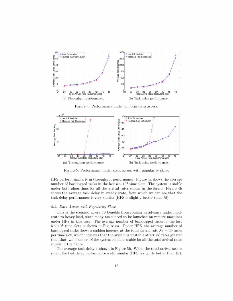
HFS perform similarly in throughput performance. Figure 4a shows the averagenumber of backlogged tasks in the last 5× 10⁴ time slots. The system is stableunder both algorithms for all the arrival rates shown in the figure. Figure 4bshows the average task delay in steady state, from which we can see that thetask delay performance is very similar (HFS is slightly better than JS).
6.2. Data Access with Popularity Skew
This is the scenario where JS benefits from routing in advance under mod-erate to heavy load, since many tasks need to be launched on remote machinesunder HFS in this case. The average number of backlogged tasks in the last5 × 104 time slots is shown in Figure 5a. Under HFS, the average number ofbacklogged tasks shows a sudden increase at the total arrival rate λΣ = 39 tasksper time slot, which indicates that the system is unstable at arrival rates greaterthan that, while under JS the system remains stable for all the total arrival ratesshown in the figure.
The average task delay is shown in Figure 5b. When the total arrival rate issmall, the task delay performance is still similar (HFS is slightly better than JS).
15
As the arrival rate increases, the task delay performance under HFS becomesworse. The average task delay under HFS becomes larger than that under JSwhen the arrival rate is greater than 35 tasks per time slot. For arrival rategreater than 39 tasks per time slot, the average task delay under HFS becomesvery large (it is already over 2000 for λΣ = 39) due to instability. Thus to get aclear comparison figure, we did not show the average task delay under HFS forarrival rate larger than 38 tasks per time slot. Overall, JS significantly reducesthe task delay under moderate to heavy load.
7. Conclusions and Future Work
We addressed the data locality problem in task scheduling by routing datain advance through the communication network in a MapReduce computingcluster. Taking both load balancing and network capacity into consideration,we proposed a scheduling/routing algorithm, named the Joint Scheduler, thatmaximizes the throughput of the system. The Joint Scheduler can be extendedimmediately to the case that tasks have different number of local machines andto communication networks with more levels of hierarchy. The Joint Schedulerrequires control of the queues on switches. Such control is not available under thecurrent Hadoop implementation, but is possible by using the emerging software-defined networking (SDN) technology [24]. Another limitation of this work isthat we focused on the throughput performance of the system and have not putmuch effort on integrating job-level scheduling. A simple approach is to integrateit in the routing step: when a queue sends data out, it selects data based on thejob information of the corresponding tasks. However, more delicate approachescan be explored to achieve different performance goals such as fairness.
With the proposed network perspective of the data locality problem, an ex-citing direction for future work is to consider more general network architectures.The structure of the connections between machines may not be a hierarchicalone, and the bandwidths of different links can be heterogeneous.
8. Acknowledgement
This work was supported in part by NSF Grant ECCS-1255425.
References
[1] J. Dean, S. Ghemawat, MapReduce: simplified data processing on largeclusters, ACM Commun. 51 (1) (2008) 107–113.
[2] K. Shvachko, H. Kuang, S. Radia, R. Chansler, The Hadoop distributed filesystem, in: IEEE Symp. Mass Storage Systems and Technologies (MSST),Incline Villiage, NV, 2010, pp. 1–10.
16

[3] S. Kavulya, J. Tan, R. Gandhi, P. Narasimhan, An analysis of traces froma production MapReduce cluster, in: Proc. IEEE/ACM Int. Conf. Cluster,Cloud and Grid Computing (CCGRID), Melbourne, Australia, 2010, pp.94–103.
[4] G. Ananthanarayanan, S. Agarwal, S. Kandula, A. Greenberg, I. Stoica,D. Harlan, E. Harris, Scarlett: coping with skewed content popularity inMapReduce clusters, in: Proc. European Conf. Computer Systems (Eu-roSys), Salzburg, Austria, 2011, pp. 287–300.
[5] L. Tassiulas, A. Ephremides, Stability properties of constrained queueingsystems and scheduling policies for maximum throughput in multihop radionetworks, IEEE Trans. Autom. Control 4 (1992) 1936–1948.
[6] M. Zaharia, D. Borthakur, J. Sen Sarma, K. Elmeleegy, S. Shenker, I. Sto-ica, Delay scheduling: a simple technique for achieving locality and fair-ness in cluster scheduling, in: Proc. European Conf. Computer Systems(EuroSys), Paris, France, 2010, pp. 265–278.
[7] M. Isard, V. Prabhakaran, J. Currey, U. Wieder, K. Talwar, A. Goldberg,Quincy: fair scheduling for distributed computing clusters, in: Proc. ACMSymp. Operating Systems Principles (SOSP), Big Sky, MT, 2009, pp. 261–276.
[8] S. Seo, I. Jang, K. Woo, I. Kim, J.-S. Kim, S. Maeng, HPMR: Prefetch-ing and pre-shuffling in shared MapReduce computation environment, in:IEEE Int. Conf. Cluster Computing (CLUSTER), New Orleans, LA, 2009,pp. 1–8.
[9] J. Jin, J. Luo, A. Song, F. Dong, R. Xiong, Bar: An efficient data lo-cality driven task scheduling algorithm for cloud computing, in: Proc.IEEE/ACM Int. Conf. Cluster, Cloud and Grid Computing (CCGRID),Newport Beach, CA, 2011, pp. 295–304.
[10] C. Abad, Y. Lu, R. Campbell, DARE: Adaptive data replication for efficientcluster scheduling, in: IEEE Int. Conf. Cluster Computing (CLUSTER),Austin, TX, 2011, pp. 159–168.
[11] Q. Xie, Y. Lu, Degree-guided map-reduce task assignment with data lo-cality constraint, in: Proc. IEEE Int. Symp. Information Theory (ISIT),Cambridge, MA, 2012, pp. 985–989.
[12] W. Wang, K. Zhu, L. Ying, J. Tan, L. Zhang, Map task scheduling inMapReduce with data locality: throughput and heavy-traffic optimality,in: Proc. IEEE Int. Conf. Computer Communications (INFOCOM), Turin,Italy, 2013, pp. 1609–1617.
[13] J. Tan, X. Meng, L. Zhang, Coupling task progress for MapReduceresource-aware scheduling, in: Proc. IEEE Int. Conf. Computer Communi-cations (INFOCOM), Turin, Italy, 2013, pp. 1618–1626.
17

[14] X. Bu, J. Rao, C.-Z. Xu, Interference and locality-aware task schedulingfor MapReduce applications in virtual clusters, in: Proc. ACM Int. Symp.High-Performance Parallel and Distributed Computing (HPDC), New YorkCity, NY, 2013, pp. 227–238.
[15] W. Wang, K. Zhu, L. Ying, J. Tan, L. Zhang, MapTask scheduling inMapReduce with data locality: Throughput and heavy-traffic optimality,IEEE/ACM Trans. Netw.To be published.
[16] K. Wang, X. Zhou, T. Li, D. Zhao, M. Lang, I. Raicu, Optimizing loadbalancing and data-locality with data-aware scheduling, in: Proc. IEEEInt. Conf. Big Data (Big Data), Washington DC, 2014, pp. 119–128.
[17] M. Sun, H. Zhuang, X. Zhou, K. Lu, C. Li, HPSO: Prefetching basedscheduling to improve data locality for MapReduce clusters, in: Int. Conf.Algorithms and Architectures for Parallel Processing (ICA3PP), Vol. 8631of Lecture Notes in Comput. Sci., Springer, 2014, pp. 82–95.
[18] W. Wang, M. Barnard, L. Ying, Decentralized scheduling with data localityfor data-parallel computation on peer-to-peer networks, in: Proc. Ann.Allerton Conf. Commununication, Control and Computing, Monticello, IL,2015.
[19] Q. Xie, Y. Lu, Priority algorithm for near-data scheduling: Throughputand heavy-traffic optimality, in: Proc. IEEE Int. Conf. Computer Commu-nications (INFOCOM), Hong Kong, China, 2015, pp. 963–972.
[20] M. Al-Fares, A. Loukissas, A. Vahdat, A scalable, commodity data centernetwork architecture, in: Proc. Ann. ACM SIGCOMM Conf., Seattle, WA,2008, pp. 63–74.
[21] L. Barroso, U. Holzle, The datacenter as a computer: An introduction tothe design of warehouse-scale machines, Synthesis Lectures on Comput.Architecture 4 (1) (2009) 1–108.
[22] R. Srikant, L. Ying, Communication Networks: An Optimization, Controland Stochastic Networks Perspective, Cambridge Univ. Press, New York,2014.
[23] M. Andrews, K. Kumaran, K. Ramanan, A. Stolyar, R. Vijayakumar,P. Whiting, Scheduling in a queueing system with asynchronously vary-ing service rates, Probab. Eng. Inf. Sci. 18 (2) (2004) 191–217.
[24] N. McKeown, T. Anderson, H. Balakrishnan, G. Parulkar, L. Peterson,J. Rexford, S. Shenker, J. Turner, OpenFlow: Enabling innovation in cam-pus networks, ACM SIGCOMM Comput. Commun. Rev. 38 (2) (2008)69–74.
18
Appendix A. Proof of Theorem 1
Proof. Consider the following Lyapunov function
V (Z(t)) =
M∑m=1
2∑i=0
(Qm,i(t))2 +
R∑r=1
2∑j=1
(Xr,j(t))2.
Then according to an extension of the Foster-Lyapunov theorem, it suffices toprove that there exists a finite set B ⊆ S and two constants δ and C with δ > 0such that for some positive integer T ≥ 1,
E[V (Z(t0 + T ))− V (Z(t))
∣∣ Z(t0) = Z]≤ −δ if Z ∈ Bc,
E[V (Z(t0 + T ))− V (Z(t))
∣∣ Z(t0) = Z]≤ C if Z ∈ B.
For each arrival rate vector λ ∈ Λo, we show that the queueing process {Z(t), t ≥0} satisfies these two conditions. For each λ ∈ Λo, since Λo is an open set, thereexists 0 < ε < 1 such that λ′ = (1 + ε)λ ∈ Λo. By the definition of Λ, thereexists a supportable λ′-admissible flow vector f ′. Let f = f ′/(1 + ε). Then fsatisfies the equations in (4), and the inequalities in (5) become∑
~L∈Lm
λ~L,m,1 ≤B1
1 + ε(A.1a)
∑m∈Mr
λm,1 ≤B2
1 + ε(A.1b)
∑r′∈R
ηr′,r ≤B2
1 + ε(A.1c)
∑m′∈Mrm
αm′,m + λm,2 ≤B1
1 + ε(A.1d)
∑~L∈Lm
λ~L,m,0 + µm ≤ϕ
1 + ε. (A.1e)
If machine m is not local for any task type in L, the states in S all have Qm,1 = 0.Thus we do not need to consider Qm,1. For such m, we also have λ~L,m,1 = 0,
λm,1 = 0, and αm,m′ = 0 for any m′. Therefore we do not consider such mwhen we write these rates in the rest of this paper. Similarly if the machines inrack r are not local for any task type in L, Xr,1 is always zero and ηr,r′ = 0 forany r′. We do not consider these terms either. Then we can find f ′ such thatother terms in the equalities in (A.1) are all positive since λ′ is in the open setΛo. Let M denote the set of machines that are local machines for some tasktype and R denote the set of racks that have local machines for some task type.
By the queue dynamics, the T time slot Lyapunov drift can be calculated as
E[V (Z(t0 + T ))− V (Z(t))
∣∣ Z(t0)]
19

= E
[t1∑t=t0
(M∑m=1
2∑i=0
((Qm,i(t+ 1))2 − (Qm,i(t))
2)
+
R∑r=1
2∑j=1
((Xr,j(t+ 1))2 − (Xr,j(t))
2)) ∣∣∣∣ Z(t0)
]
≤ E
[∑t
(∑m
( ∑~L∈Lm
A~L,m,1(t)− Sm,1(t))2
+∑m
( ∑~L∈Lm
A~L,m,0(t) +Am,0(t)− Sm(t))2
+∑m
(Am,2(t) +
∑m′∈Mrm
AQm′,m(t)− Sm,2(t))2
+∑r
( ∑m∈Mr
Am,1(t)− SXr,1(t))2
+∑r
(∑r′∈R
AXr′,r(t)− SXr,2(t))2) ∣∣∣∣ Z(t0)
]
+ 2E[∑
t
(∑m
Qm,1(t)( ∑~L∈Lm
A~L,m,1(t)− Sm,1(t))
+∑m
Qm,0(t)( ∑~L∈Lm
A~L,m,0(t) +Am,0(t)− Sm(t))
+∑m
Qm,2(t)(Am,2(t) +
∑m′∈Mrm
AQm′,m(t)− Sm,2(t))
+∑r
Xr,1(t)( ∑m∈Mr
Am,1(t)− SXr,1(t))2
+∑r
Xr,2(t)(∑r′∈R
AXr′,r(t)− SXr,2(t))) ∣∣∣ Z(t0)
], (A.2)
where t1 = t0 +T −1 and the summation ranges may be omitted when they areclear from context. The first expectation term in the right-hand side of (A.2)can be bounded for all states Z(t0) by a constant, say C1, since the arrivalprocesses have finite second moments and the service processes are bounded.For the second expectation term in the right-hand side of (A.2), we denote itby 2E
[H|Z(t0)
]and rewrite H as follows.
H =∑t
∑m
∑~L∈Lm
(Qm,1(t)A~L,m,1(t) +Qm,0(t)A~L,m,0(t)
)(A.3)
+∑t
(∑r
Xr,1(t)∑
m∈Mr
Am,1(t)
20

+∑m
Qm,2(t)∑
m′∈Mrm
AQm′,m(t)
−∑m
Qm,1(t)Sm,1(t))
(A.4)
+∑t
(∑r
Xr,2(t)∑r′∈R
Ar′,r(t)−∑r
Xr,1(t)SXr,1(t))
(A.5)
+∑t
(∑m
Qm,2(t)Am,2(t)−∑r
Xr,2(t)SXr,2(t))
(A.6)
+∑t
∑m
(Qm,0(t)Am,0(t)−Qm,2(t)Sm,2(t)
)(A.7)
−∑t
∑m
Qm,0(t)Sm(t). (A.8)
Next we take expectations and bound these terms.For term (A.3), exchanging the order of summation yields∑
m
∑~L∈Lm
(Qm,1(t)A~L,m,1(t) +Qm,0(t)A~L,m,0(t)
)=∑~L
∑m∈M~L
(Qm,1(t)A~L,m,1(t) +Qm,0(t)A~L,m,0(t)
)According to the task assignment policy for new tasks, for each ~L, all the A~L(t)arrivals are assigned to the shortest queue in Q~L. Denote this shortest queueby Dt
~L. Then∑
m∈M~L
(Qm,1(t)A~L,m,1(t) +Qm,0(t)A~L,m,0(t)
)= Dt
~L(t)A~L(t).
Since {Z(t), t ≥ 0} is a Markov chain, we have
E[∑m
∑~L∈Lm
(Qm,1(t)A~L,m,1(t) +Qm,0(t)A~L,m,0(t)
) ∣∣∣∣ Z(t0)
]
= E
[E[∑~L
Dt~L
(t)A~L
∣∣∣∣ Z(t)
] ∣∣∣∣∣ Z(t0)
]
= E[∑~L
Dt~L
(t)λ~L
∣∣∣∣ Z(t0)
](a)
≤ E[∑~L
∑m∈M~L
(Qm,1(t)λ~L,m,1 +Qm,0(t)λ~L,m,0
) ∣∣∣∣ Z(t0)
]
= E[∑m
∑~L∈Lm
(Qm,1(t)λ~L,m,1 +Qm,0(t)λ~L,m,0
) ∣∣∣∣ Z(t0)
], (A.9)
21

where (a) follows from flow conservation equation (4a) and the fact that Dt~L
isthe shortest queue in Q~L at time slot t. The following two terms will be usedin the rest of the proof. ∑
t
∑m
Qm,1(t)∑~L∈Lm
λ~L,m,1 (A.10a)
∑t
∑m
Qm,0(t)∑~L∈Lm
λ~L,m,0. (A.10b)
For term (A.4), first notice that∑m
Qm,2(t)∑
m′∈Mrm
AQm′,m(t)
=∑m′
∑m∈Mr
m′
Qm,2(t)AQm′,m(t)
=∑m
∑m′∈Mrm
Qm′,2(t)AQm,m′(t),
where we have changed the order of summation and swapped the names ofdummy variables m and m′. Then the arrival part can be written as∑
r
Xr,1(t)∑
m∈Mr
Am,1(t) +∑m
Qm,2(t)∑
m′∈Mrm
AQm′,m(t)
=∑m
(Xrm,1(t)Am,1(t) +
∑m′∈Mrm
Qm′,2(t)AQm,m′(t)).
According to the routing policy, the departures of queue Qm,1 are all routed toDt−1Qm,1
at time slot t, where Dt−1Qm,1
is the shortest queue in DQm,1at time slot
t− 1. By the relation (2a),∑m
(Xrm,1(t)Am,1(t) +
∑m′∈Mrm
Qm′,2(t)AQm,m′(t))
≤∑m
Dt−1Qm,1
(t)Sm,1(t− 1).
We bound this term as follows using Lemma 2 provided after this proof, whichresults from the queue dynamics:∑
t
∑m
Dt−1Qm,1
(t)Sm,1(t− 1)
≤∑t
∑m
DtQm,1
(t)Sm,1(t) +B2
∑m
Dt0Qm,1
(t0)
+MB2T
t1∑t=t0
∑~L
A~L(t) + 2M2B22T
2
22
≤∑t
∑m
DtQm,1
(t)Sm,1(t) +B2
∑r
Xr,1(t0)
+MB2T
t1∑t=t0
∑~L
A~L(t) + 2M2B22T
2,
Therefore
(A.4) ≤∑t
∑m
(DtQm,1
(t)−Qm,1(t))Sm,1(t)
+B2
∑r
Xr,1(t0) + +MB2T
t1∑t=t0
∑~L
A~L(t) + 2M2B22T
2.
Next we combine (A.4) with (A.10a) and consider the following two cases. WhenDtQm,1
(t) < Qm,1(t), by queue dynamics Sm,1(t) = B1. Then(DtQm,1
(t)−Qm,1(t))Sm,1(t) +Qm,1(t)
∑~L∈Lm
λ~L,m,1
= DtQm,1
(t)1 + ε
1 + ε/2
∑~L∈Lm
λ~L,m,1
+DtQm,1
(t)(B1 −
1 + ε
1 + ε/2
∑~L∈Lm
λ~L,m,1
)−Qm,1(t)
(B1 −
∑~L∈Lm
λ~L,m,1
)(a)< Dt
Qm,1(t)
1 + ε
1 + ε/2
∑~L∈Lm
λ~L,m,1
+Qm,1(t)(B1 −
1 + ε
1 + ε/2
∑~L∈Lm
λ~L,m,1
)−Qm,1(t)
(B1 −
∑~L∈Lm
λ~L,m,1
)= Dt
Qm,1(t)
1 + ε
1 + ε/2
∑~L∈Lm
λ~L,m,1
−Qm,1(t)ε/2
1 + ε/2
∑~L∈Lm
λ~L,m,1,
where (a) is true since DtQm,1
(t) < Qm,1(t) and by (A.1a)
1 + ε
1 + ε/2
∑~L∈Lm
λ~L,m,1 ≤1
1 + ε/2B1 < B1.
23

When DtQm,1
(t) ≥ Qm,1(t), by definition Sm,1(t) = 0. Then(DtQm,1
(t)−Qm,1(t))Sm,1(t) +Qm,1(t)
∑~L∈Lm
λ~L,m,1
= Qm,1(t)( 1 + ε
1 + ε/2
∑~L∈Lm
λ~L,m,1 −ε/2
1 + ε/2
∑~L∈Lm
λ~L,m,1
)≤ Dt
Qm,1(t)
1 + ε
1 + ε/2
∑~L∈Lm
λ~L,m,1
−Qm,1(t)ε/2
1 + ε/2
∑~L∈Lm
λ~L,m,1.
In both cases we get the same upper bound. Further by the flow conservationequation (4b) we have∑
m
DtQm,1
(t)1 + ε
1 + ε/2
∑~L∈Lm
λ~L,m,1
=1 + ε
1 + ε/2
∑m
DtQm,1
(t)(λm,1 +
∑m′∈Mrm
αm,m′
)≤ 1 + ε
1 + ε/2
∑m
(Xrm,1(t)λm,1 +
∑m′∈Mrm
Qm′,2(t)αm,m′
)=∑r
Xr,1(t)1 + ε
1 + ε/2
∑m∈Mr
λm,1
+∑m
Qm,2(t)1 + ε
1 + ε/2
∑m′∈Mrm
αm′,m.
Thus combining (A.4) with (A.10a) yields∑t
(∑m
Qm,1(t)∑~L∈Lm
λ~L,m,1 +∑r
Xr,1(t)∑
m∈Mr
Am,1(t)
+∑m
Qm,2(t)∑
m′∈Mrm
AQm′,m(t)−∑m
Qm,1(t)Sm,1(t))
≤∑t
∑r
Xr,1(t)1 + ε
1 + ε/2
∑m∈Mr
λm,1 (A.11a)
+∑t
∑m
Qm,2(t)1 + ε
1 + ε/2
∑m′∈Mrm
αm′,m (A.11b)
−∑t
∑m
Qm,1(t)ε/32
1 + ε/16
∑~L∈Lm
λ~L,m,1 (A.11c)
+B2
∑r
Xr,1(t0) +MB2T
t1∑t=t0
∑~L
A~L(t) + 2M2B22T
2, (A.11d)
24
where we have used the fact
ε/2
1 + ε/2>
ε/32
1 + ε/16.
For terms (A.5)–(A.7), we use similar techniques as we have used for term(A.4). We omit the details and list the bounds as follows.
(A.11a) + (A.5) ≤∑t
∑r
Xr,2(t)1 + ε/2
1 + ε/4
∑r′∈R
ηr′,r (A.12a)
−∑t
∑r
Xr,1(t)ε/32
1 + ε/16
∑m∈Mr
λm,1 (A.12b)
+B2
∑r
Xr,2(t0) +RB2T
t1∑t=t0
∑~L
A~L(t) (A.12c)
+ 2RMB22T
2. (A.12d)
(A.12a) + (A.6) ≤∑t
∑m
Qm,2(t)1 + ε/4
1 + ε/8λm,2 (A.13a)
−∑t
∑r
Xr,2(t)ε/32
1 + ε/16
∑r′∈R
ηr′,r (A.13b)
+B2
∑m
Qm,2(t0) +RB2T
t1∑t=t0
∑~L
A~L(t) (A.13c)
+ 2RMB22T
2. (A.13d)
(A.11b) + (A.13a) + (A.7) ≤∑t
∑m
Qm,0(t)1 + ε/8
1 + ε/16µm (A.14a)
−∑t
∑m
Qm,2(t)ε/32
1 + ε/16
(λm,2 +
∑m′∈Mrm
αm′,m
)(A.14b)
+B2
∑m
Qm,0(t0) +MB2T
t1∑t=t0
∑~L
A~L(t) + 2M2B22T
2. (A.14c)
For the last term (A.8), we combine (A.10b) and (A.14a) with (A.8) andtake expectations as follows.
E[Qm,0(t)
( ∑~L∈Lm
λ~L,m,0 +1 + ε/8
1 + ε/16µm − Sm(t)
) ∣∣∣∣ Z(t0)
]
= E
[E[Qm,0(t)
( ∑~L∈Lm
λ~L,m,0 +1 + ε/8
1 + ε/16µm
) ∣∣∣∣ Z(t)
]
25

− E[Qm,0(t)Sm(t)
∣∣∣∣ Z(t)
] ∣∣∣∣∣ Z(t0)
]
= E[Qm,0(t)
( ∑~L∈Lm
λ~L,m,0 +1 + ε/8
1 + ε/16µm − ϕ)
) ∣∣∣∣ Z(t0)
]
≤ −E[Qm,0(t)
1
1 + ε
1 + ε/8
1 + ε/16ϕ
∣∣∣∣ Z(t0)
]≤ −E
[Qm,0(t)
ε/32
1 + ε/16ϕ
∣∣∣∣ Z(t0)
]. (A.15)
Let
ρ = min
{ϕ,{ ∑~L∈Lm
λ~L,m,1
∣∣∣ m ∈M}{ ∑m∈Mr
λm,1
∣∣∣ r ∈ R}{∑r′
ηr′,r
∣∣∣ r = 1, · · · , R}
{λm,2 +
∑m′∈Mrm
αm′,m
∣∣∣ m = 1, · · · ,M}}
.
Then by the selection of f we have ρ > 0. Finally combining all the terms yields
E[H | Z(t0)] ≤ − ε/32
1 + ε/16ρ
t1∑t=t0
E[ M∑m=0
2∑i=0
Qm,i(t)∣∣∣ Z(t0)
]
− ε/32
1 + ε/16ρ
t1∑t=t0
E[ R∑r=0
2∑j=1
Xr,j(t)∣∣∣ Z(t0)
]
+B2
( M∑m=0
2∑i=0
Qm,i(t0) +
R∑r=0
2∑j=1
Xr,j(t0))
+ 2(M +R)B2T
t1∑t=t0
∑~L
λ~L + 4(M +R)MB22T
2.
For each t0 ≤ t ≤ t1, due to the boundedness of departures of each queue,
Qm,i(t) ≥ Qm,i(t0)−B1T
Xr,j(t) ≥ Xr,j(t0)−B2T.
Therefore
E[H | Z(t0)] ≤(− ε/32
1 + ε/16ρT +B2
)26

·( M∑m=0
2∑i=0
Qm,i(t0) +
R∑r=0
2∑j=1
Xr,j(t0))
+ C2,
where
C2 = 2(M +R)B2T
t1∑t=t0
∑~L
λ~L + 4(M +R)MB22T
2 + ρT (3MB1T + 2RB2T ).
Let
T >2B2(1 + ε/16)
ρε/32.
Then
E[H|Z(t0)] ≤−B2
( M∑m=0
2∑i=0
Qm,i(t0) +
R∑r=0
2∑j=1
Xr,j(t0))
+ C2.
Hence
E[V (Z(t0 + T ))− V (Z(t))
∣∣ Z(t0)]
≤ −2B2
( M∑m=0
2∑i=0
Qm,i(t0) +
R∑r=0
2∑j=1
Xr,j(t0))
+ C1 + 2C2.
Pick δ > 0 and let
B =
{Z∣∣∣ M∑m=0
2∑i=0
Qm,i +
R∑r=0
2∑j=1
Xr,j <δ + C1 + 2C2
2B2
},
and C = C1 + 2C2. Then B is a finite set and
E[V (Z(t0 + T ))− V (Z(t))
∣∣ Z(t0) = Z]≤ −δ if Z ∈ Bc,
E[V (Z(t0 + T ))− V (Z(t))
∣∣ Z(t0) = Z]≤ C if Z ∈ B,
which completes the proof.
Lemma 2. For any queue Q in the communication network, let DtQ be the
shortest queue in DQ at time slot t and S(t) be the service defined in queuedynamics. Then
t1∑t=t0
Dt−1Q (t)S(t− 1) ≤
t1∑t=t0
DtQ(t)S(t) +B2D
t0Q (t0)
+B2T
t1∑t=t0
∑~L
A~L(t) + 2MB22T
2,
where t1 = t0 + T − 1.
27
Proof. The number of arrivals to any queue Q at any time slot t is upperbounded by
∑~LA~L(t). Due to the boundedness of departures, for any t such
that t0 ≤ t ≤ t1 we have
Dt−1Q (t) ≤ Dt−1
Q (t− 1) +∑~L
A~L(t) +MB2 (A.16)
≤ Dt0Q (t− 1) +
∑~L
A~L(t) +MB2 (A.17)
≤ Dt0Q (t0) +
t1∑t=t0
∑~L
A~L(t) +MB2T, (A.18)
where (A.17) is true since Dt−1Q (t− 1) is the shortest queue in DQ at time slot
t− 1. Then∑t
Dt−1Q (t)S(t− 1) (A.19)
≤∑t
Dt0Q (t0)S(t− 1) +B2T
t1∑t=t0
∑~L
A~L(t) +MB22T
2 (A.20)
= Dt0Q (t0)
∑t
S(t− 1) +B2T
t1∑t=t0
∑~L
A~L(t) +MB22T
2 (A.21)
≤ Dt0Q (t0)
∑t
S(t) +B2Dt0Q (t0) +B2T
t1∑t=t0
∑~L
A~L(t) +MB22T
2, (A.22)
where (A.22) follows from that∑t S(t− 1) ≤
∑t S(t) +B2. Similarly we have
the following inequalities for any t0 ≤ t ≤ t1:
Dt0Q (t0) ≤ Dt
Q(t0) ≤ DtQ(t) +MB2T. (A.23)
Inserting the above inequality to (A.22) gives∑t
Dt−1Q (t)S(t− 1) ≤
∑t
DtQ(t)S(t) +B2D
t0Q (t0) (A.24)
+B2T
t1∑t=t0
∑~L
A~L(t) + 2MB22T
2, (A.25)
which completes the proof.
28