DATA MININGLECTURE 7Hierarchical Clustering, DBSCAN

The EM Algorithm

CLUSTERING

What is a Clustering?• In general a grouping of objects such that the objects in a

group (cluster) are similar (or related) to one another and different from (or unrelated to) the objects in other groups

Inter-cluster distances are maximized

Intra-cluster distances are

minimized

Clustering Algorithms

• K-means and its variants

• Hierarchical clustering

• DBSCAN

HIERARCHICAL CLUSTERING

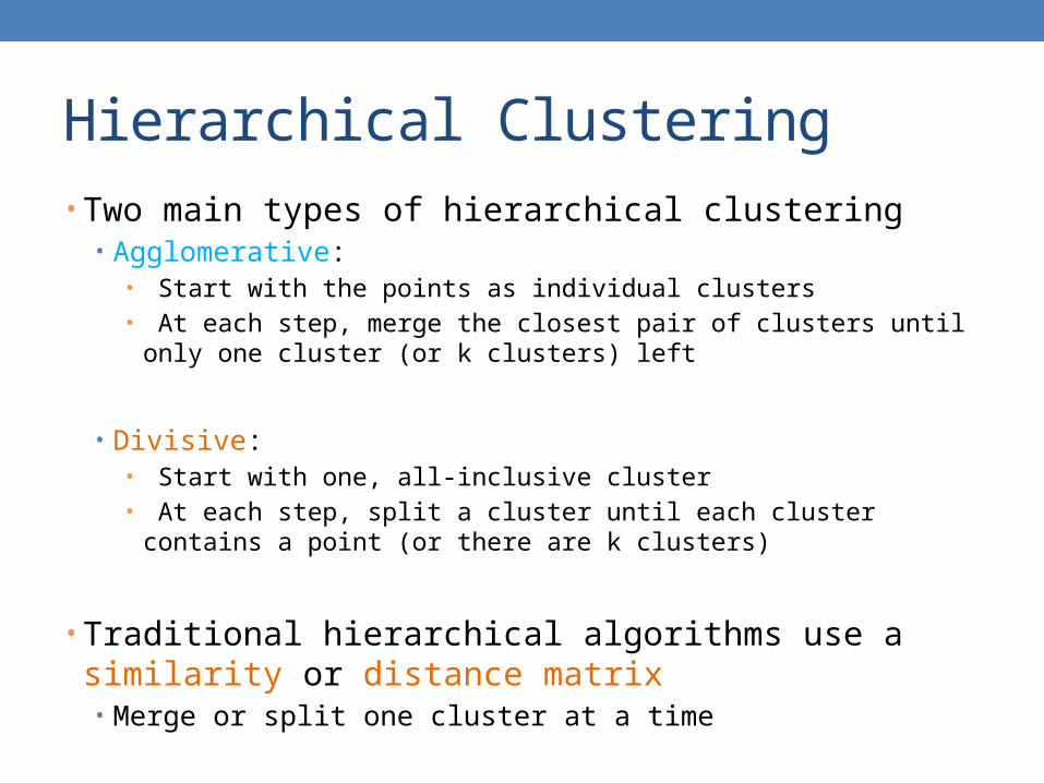
Hierarchical Clustering• Two main types of hierarchical clustering

• Agglomerative: • Start with the points as individual clusters• At each step, merge the closest pair of clusters until only one cluster (or

k clusters) left

• Divisive: • Start with one, all-inclusive cluster • At each step, split a cluster until each cluster contains a point (or there

are k clusters)

• Traditional hierarchical algorithms use a similarity or distance matrix• Merge or split one cluster at a time

Hierarchical Clustering

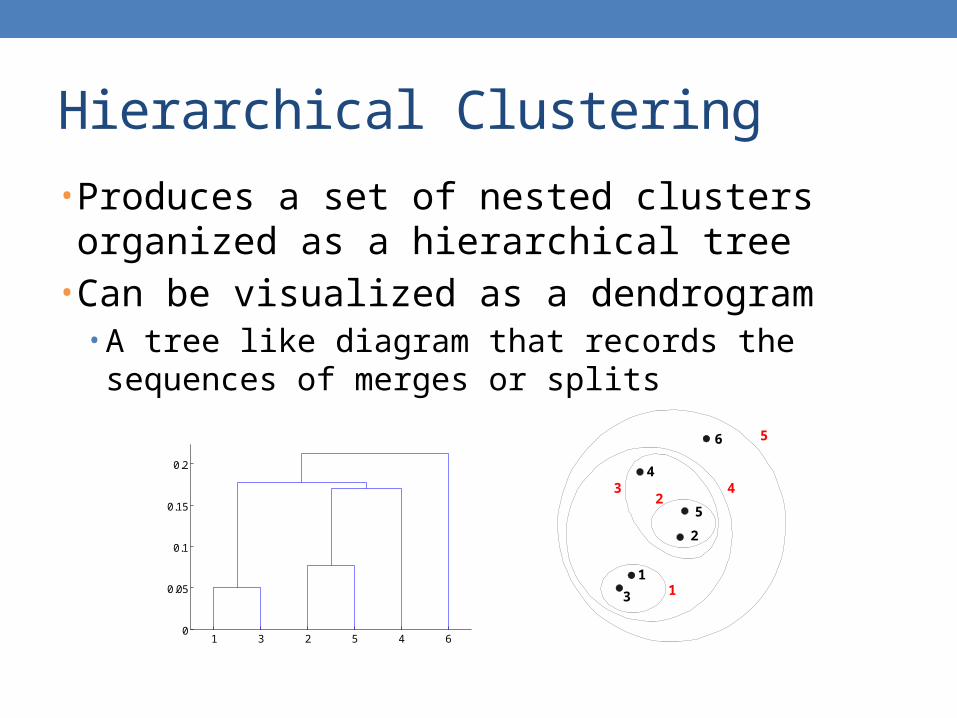
• Produces a set of nested clusters organized as a hierarchical tree

• Can be visualized as a dendrogram• A tree like diagram that records the sequences of

merges or splits

1 3 2 5 4 60

0.05

0.1

0.15

0.2

1

2

3

4

5

6

1

23 4

5

Strengths of Hierarchical Clustering• Do not have to assume any particular number of clusters• Any desired number of clusters can be obtained by

‘cutting’ the dendogram at the proper level

• They may correspond to meaningful taxonomies• Example in biological sciences (e.g., animal kingdom,

phylogeny reconstruction, …)

Agglomerative Clustering Algorithm• More popular hierarchical clustering technique

• Basic algorithm is straightforward1. Compute the proximity matrix2. Let each data point be a cluster3. Repeat4. Merge the two closest clusters5. Update the proximity matrix6. Until only a single cluster remains

• Key operation is the computation of the proximity of two clusters

• Different approaches to defining the distance between clusters distinguish the different algorithms

Starting Situation • Start with clusters of individual points and a proximity matrix

p1

p3

p5

p4

p2

p1 p2 p3 p4 p5 . . .

.

.

. Proximity Matrix

...p1 p2 p3 p4 p9 p10 p11 p12

Intermediate Situation• After some merging steps, we have some clusters

C1

C4

C2 C5

C3

C2C1

C1

C3

C5

C4

C2

C3 C4 C5

Proximity Matrix

...p1 p2 p3 p4 p9 p10 p11 p12

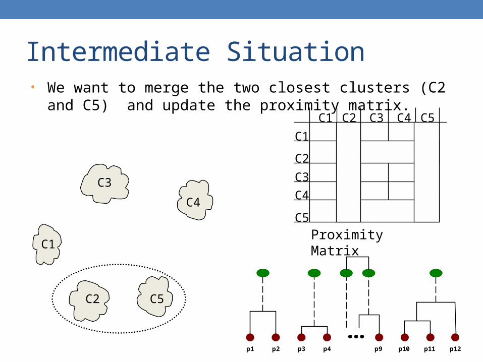
Intermediate Situation• We want to merge the two closest clusters (C2 and C5) and

update the proximity matrix.

C1

C4

C2 C5

C3

C2C1

C1

C3

C5

C4

C2

C3 C4 C5

Proximity Matrix

...p1 p2 p3 p4 p9 p10 p11 p12

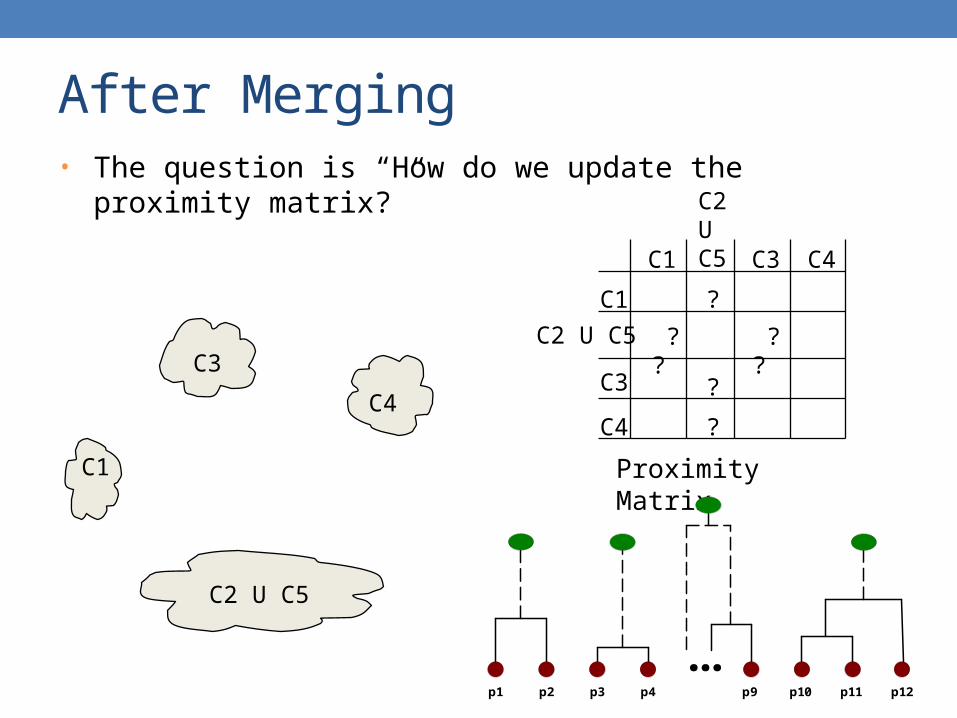
After Merging• The question is “How do we update the proximity matrix?”

C1

C4

C2 U C5

C3 ? ? ? ?

?

?

?

C2 U C5C1

C1

C3

C4

C2 U C5

C3 C4

Proximity Matrix

...p1 p2 p3 p4 p9 p10 p11 p12

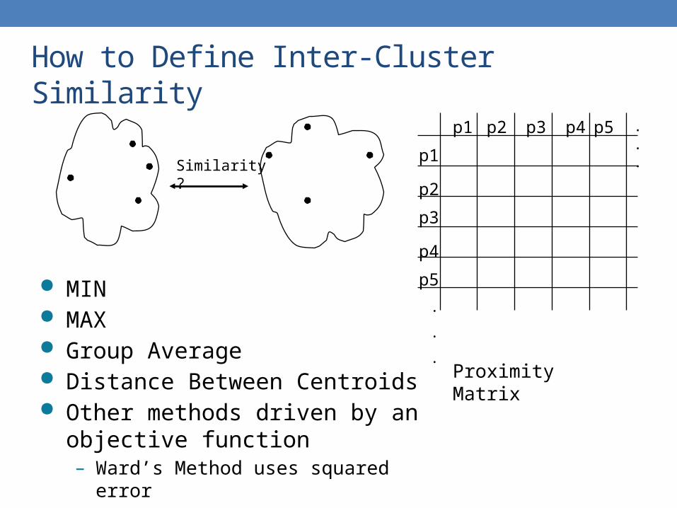
How to Define Inter-Cluster Similarity

p1

p3

p5

p4

p2

p1 p2 p3 p4 p5 . . .

.

.

.

Similarity?

MIN MAX Group Average Distance Between Centroids Other methods driven by an objective

function– Ward’s Method uses squared error

Proximity Matrix

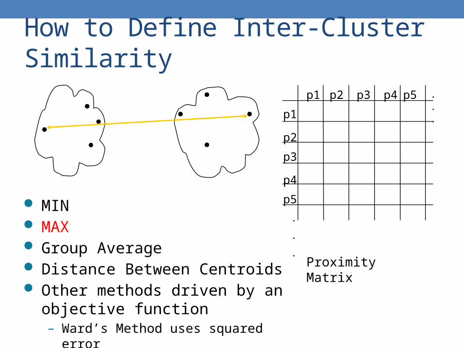
How to Define Inter-Cluster Similarity

p1

p3

p5

p4

p2

p1 p2 p3 p4 p5 . . .

.

.

.Proximity Matrix

MIN MAX Group Average Distance Between Centroids Other methods driven by an objective

function– Ward’s Method uses squared error

How to Define Inter-Cluster Similarity

p1

p3

p5

p4

p2

p1 p2 p3 p4 p5 . . .

.

.

.Proximity Matrix

MIN MAX Group Average Distance Between Centroids Other methods driven by an objective

function– Ward’s Method uses squared error

How to Define Inter-Cluster Similarity

p1

p3

p5

p4

p2

p1 p2 p3 p4 p5 . . .

.

.

.Proximity Matrix

MIN MAX Group Average Distance Between Centroids Other methods driven by an objective

function– Ward’s Method uses squared error

How to Define Inter-Cluster Similarity

p1

p3

p5

p4

p2

p1 p2 p3 p4 p5 . . .

.

.

.Proximity Matrix

MIN MAX Group Average Distance Between Centroids Other methods driven by an objective

function– Ward’s Method uses squared error

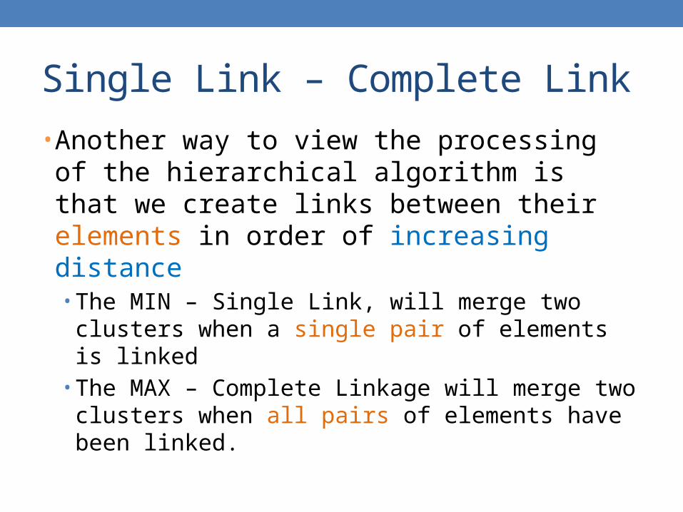
Single Link – Complete Link

• Another way to view the processing of the hierarchical algorithm is that we create links between their elements in order of increasing distance• The MIN – Single Link, will merge two clusters when a

single pair of elements is linked• The MAX – Complete Linkage will merge two clusters

when all pairs of elements have been linked.

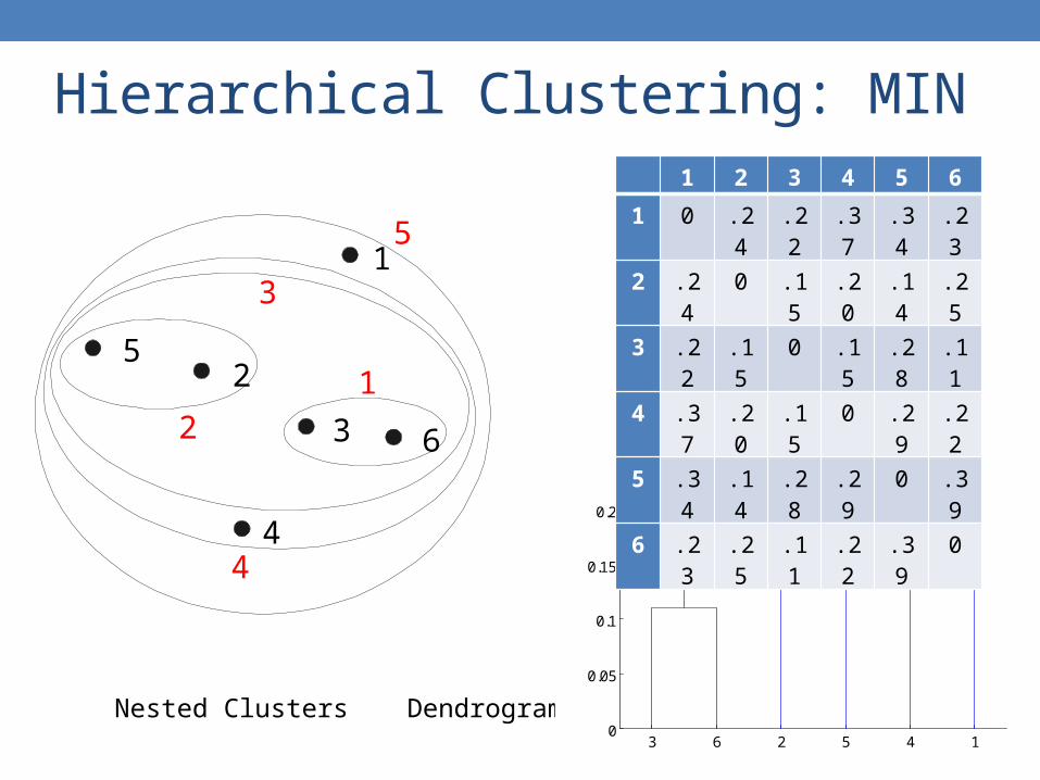
Hierarchical Clustering: MIN

Nested Clusters Dendrogram

1

2

3

4

5

6

1

2

3

4

5

3 6 2 5 4 10

0.05

0.1

0.15

0.2

1 2 3 4 5 6

1 0 .24 .22 .37 .34 .23

2 .24 0 .15 .20 .14 .25

3 .22 .15 0 .15 .28 .11

4 .37 .20 .15 0 .29 .22

5 .34 .14 .28 .29 0 .39

6 .23 .25 .11 .22 .39 0

Strength of MIN

Original Points Two Clusters

• Can handle non-elliptical shapes

Limitations of MIN

Original Points Two Clusters

• Sensitive to noise and outliers

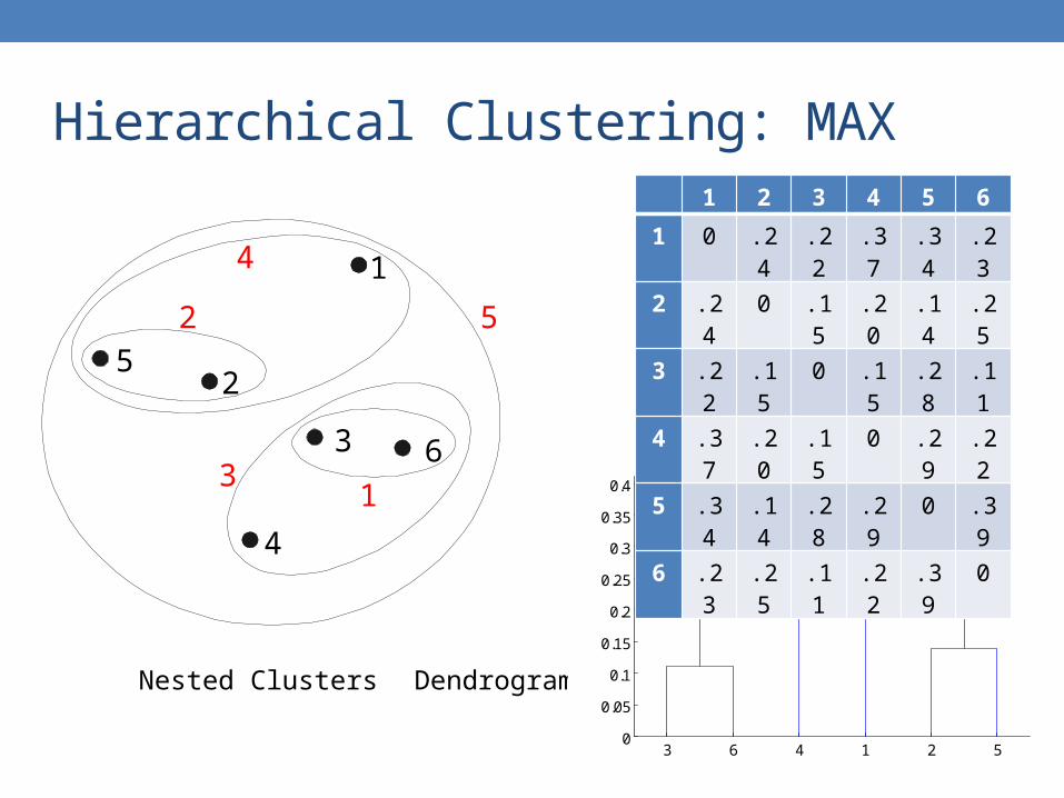
Hierarchical Clustering: MAX

Nested Clusters Dendrogram

3 6 4 1 2 50

0.05

0.1

0.15

0.2

0.25

0.3

0.35

0.4

1

2

3

4

5

6

1

2 5

3

4

1 2 3 4 5 6

1 0 .24 .22 .37 .34 .23

2 .24 0 .15 .20 .14 .25

3 .22 .15 0 .15 .28 .11

4 .37 .20 .15 0 .29 .22

5 .34 .14 .28 .29 0 .39

6 .23 .25 .11 .22 .39 0

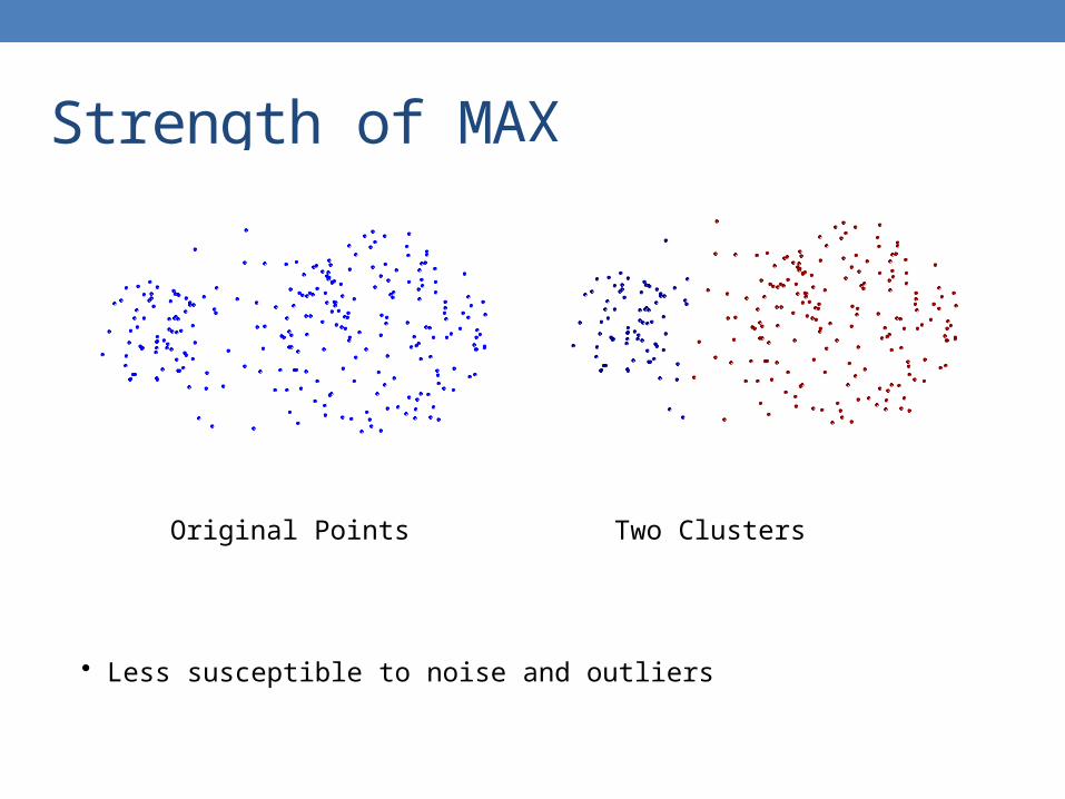
Strength of MAX

Original Points Two Clusters

• Less susceptible to noise and outliers

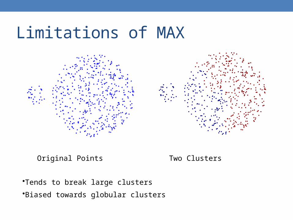
Limitations of MAX

Original Points Two Clusters

•Tends to break large clusters

•Biased towards globular clusters

Cluster Similarity: Group Average• Proximity of two clusters is the average of pairwise proximity

between points in the two clusters.

• Need to use average connectivity for scalability since total proximity favors large clusters

||Cluster||Cluster

)p,pproximity(

)Cluster,Clusterproximity(ji

ClusterpClusterp

ji

jijjii

1 2 3 4 5 6

1 0 .24 .22 .37 .34 .23

2 .24 0 .15 .20 .14 .25

3 .22 .15 0 .15 .28 .11

4 .37 .20 .15 0 .29 .22

5 .34 .14 .28 .29 0 .39

6 .23 .25 .11 .22 .39 0

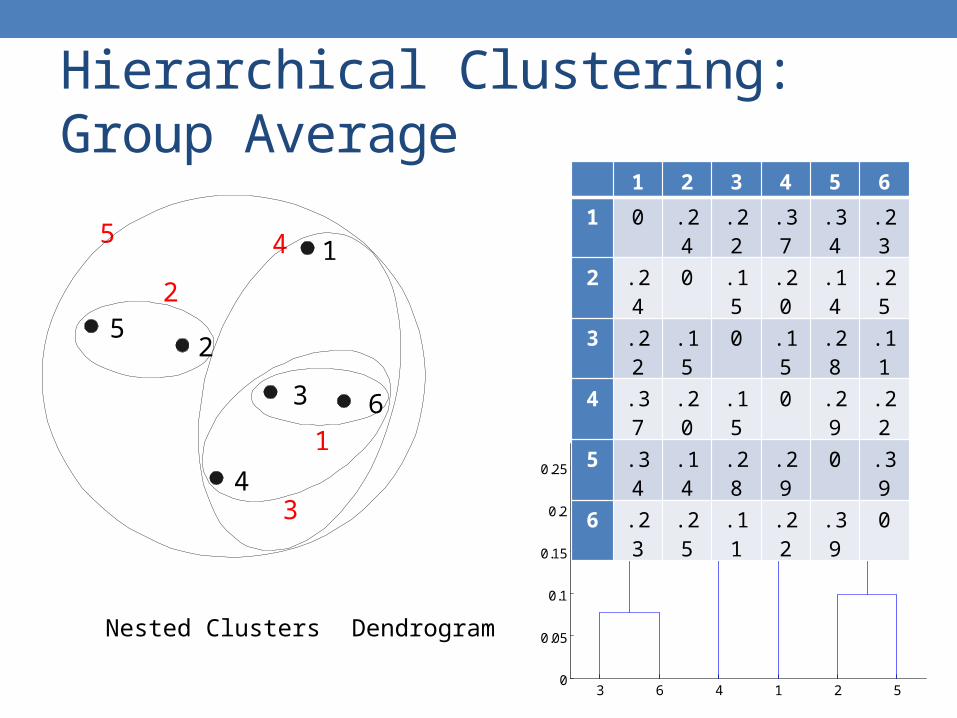
Hierarchical Clustering: Group Average

Nested Clusters Dendrogram

3 6 4 1 2 50

0.05

0.1

0.15

0.2

0.25

1

2

3

4

5

6

1

2

5

3

4

1 2 3 4 5 6

1 0 .24 .22 .37 .34 .23

2 .24 0 .15 .20 .14 .25

3 .22 .15 0 .15 .28 .11

4 .37 .20 .15 0 .29 .22

5 .34 .14 .28 .29 0 .39

6 .23 .25 .11 .22 .39 0

Hierarchical Clustering: Group Average

• Compromise between Single and Complete Link

• Strengths• Less susceptible to noise and outliers

• Limitations• Biased towards globular clusters

Cluster Similarity: Ward’s Method

• Similarity of two clusters is based on the increase in squared error (SSE) when two clusters are merged• Similar to group average if distance between points is

distance squared

• Less susceptible to noise and outliers

• Biased towards globular clusters

• Hierarchical analogue of K-means• Can be used to initialize K-means

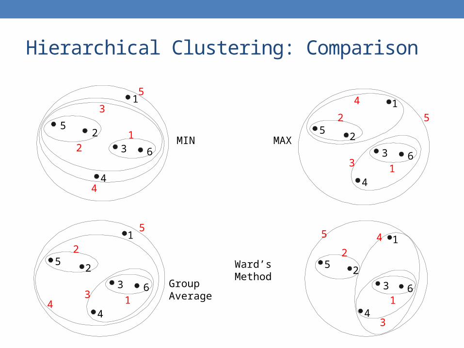
Hierarchical Clustering: Comparison

Group Average

Ward’s Method

1

2

3

4

5

61

2

5

3

4

MIN MAX

1

2

3

4

5

61

2

5

34

1

2

3

4

5

61

2 5

3

41

2

3

4

5

6

12

3

4

5

Hierarchical Clustering: Time and Space requirements

• O(N2) space since it uses the proximity matrix. • N is the number of points.

• O(N3) time in many cases• There are N steps and at each step the size, N2,

proximity matrix must be updated and searched• Complexity can be reduced to O(N2 log(N) ) time for

some approaches

Hierarchical Clustering: Problems and Limitations• Computational complexity in time and space

• Once a decision is made to combine two clusters, it cannot be undone

• No objective function is directly minimized

• Different schemes have problems with one or more of the following:• Sensitivity to noise and outliers• Difficulty handling different sized clusters and convex shapes• Breaking large clusters

DBSCAN

DBSCAN: Density-Based Clustering• DBSCAN is a Density-Based Clustering algorithm

• Reminder: In density based clustering we partition points into dense regions separated by not-so-dense regions.

• Important Questions:• How do we measure density?• What is a dense region?

• DBSCAN:• Density at point p: number of points within a circle of radius Eps• Dense Region: A circle of radius Eps that contains at least MinPts

points

DBSCAN• Characterization of points

• A point is a core point if it has more than a specified number of points (MinPts) within Eps• These points belong in a dense region and are at the interior

of a cluster

• A border point has fewer than MinPts within Eps, but is in the neighborhood of a core point.

• A noise point is any point that is not a core point or a border point.

DBSCAN: Core, Border, and Noise Points

DBSCAN: Core, Border and Noise Points

Original PointsPoint types: core, border and noise

Eps = 10, MinPts = 4

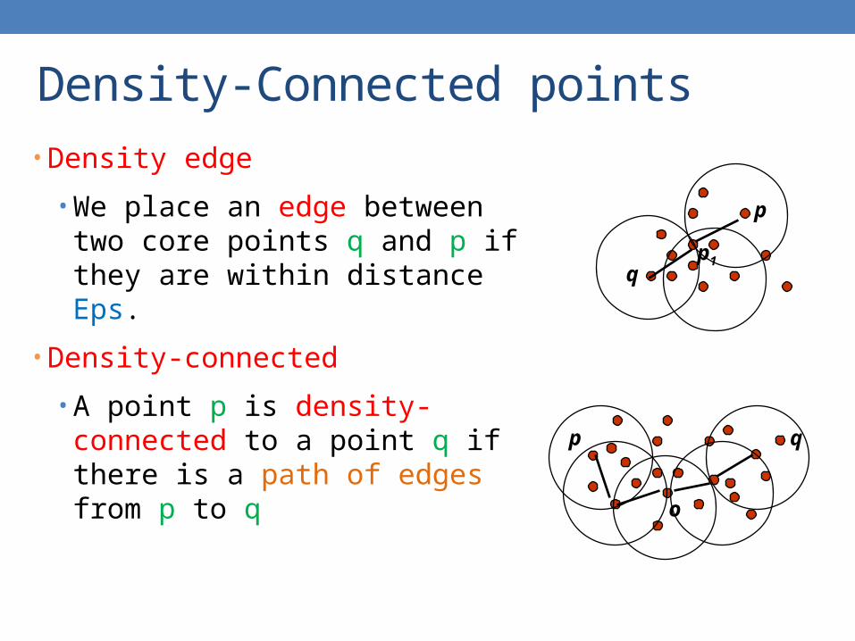
Density-Connected points• Density edge

• We place an edge between two core points q and p if they are within distance Eps.

• Density-connected

• A point p is density-connected to a point q if there is a path of edges from p to q

p

qp1

p q

o

DBSCAN Algorithm

• Label points as core, border and noise• Eliminate noise points• For every core point p that has not been assigned to a cluster• Create a new cluster with the point p and all the points that are density-connected to p.

• Assign border points to the cluster of the closest core point.

DBSCAN: Determining Eps and MinPts• Idea is that for points in a cluster, their kth nearest neighbors are

at roughly the same distance• Noise points have the kth nearest neighbor at farther distance• So, plot sorted distance of every point to its kth nearest neighbor• Find the distance d where there is a “knee” in the curve

• Eps = d, MinPts = k

Eps ~ 7-10MinPts = 4

When DBSCAN Works Well

Original PointsClusters

• Resistant to Noise

• Can handle clusters of different shapes and sizes

When DBSCAN Does NOT Work Well

Original Points

(MinPts=4, Eps=9.75).

(MinPts=4, Eps=9.92)

• Varying densities

• High-dimensional data

DBSCAN: Sensitive to Parameters

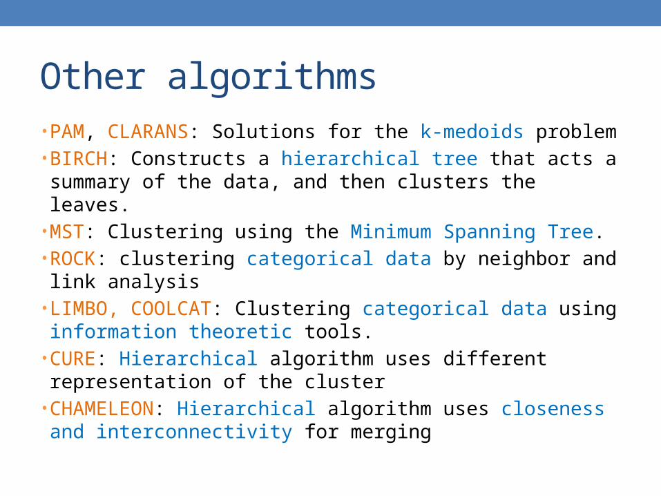
Other algorithms• PAM, CLARANS: Solutions for the k-medoids problem• BIRCH: Constructs a hierarchical tree that acts a

summary of the data, and then clusters the leaves.• MST: Clustering using the Minimum Spanning Tree.• ROCK: clustering categorical data by neighbor and link

analysis• LIMBO, COOLCAT: Clustering categorical data using

information theoretic tools.• CURE: Hierarchical algorithm uses different

representation of the cluster• CHAMELEON: Hierarchical algorithm uses closeness and

interconnectivity for merging

MIXTURE MODELS AND THE EM ALGORITHM

Model-based clustering• In order to understand our data, we will assume that there is

a generative process (a model) that creates/describes the data, and we will try to find the model that best fits the data.• Models of different complexity can be defined, but we will assume

that our model is a distribution from which data points are sampled• Example: the data is the height of all people in Greece

• In most cases, a single distribution is not good enough to describe all data points: different parts of the data follow a different distribution• Example: the data is the height of all people in Greece and China• We need a mixture model• Different distributions correspond to different clusters in the data.

Gaussian Distribution

• Example: the data is the height of all people in Greece• Experience has shown that this data follows a Gaussian

(Normal) distribution• Reminder: Normal distribution:

• = mean, = standard deviation

𝑃 (𝑥 )= 1√2𝜋 𝜎

𝑒−

(𝑥−𝜇 )2

2𝜎 2

Gaussian Model

• What is a model?• A Gaussian distribution is fully defined by the mean and

the standard deviation • We define our model as the pair of parameters

• This is a general principle: a model is defined as a vector of parameters

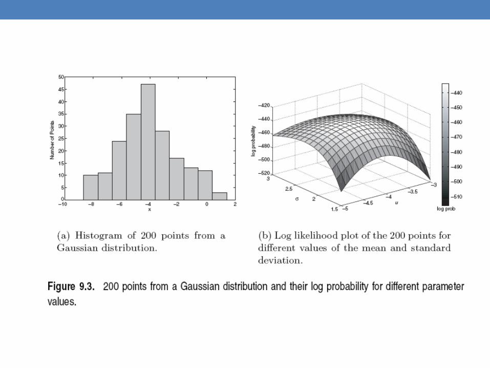
Fitting the model

• We want to find the normal distribution that best fits our data• Find the best values for and • But what does best fit mean?

Maximum Likelihood Estimation (MLE)

• Suppose that we have a vector of values• And we want to fit a Gaussian model to the data• Probability of observing point :

• Probability of observing all points (assume independence)

• We want to find the parameters that maximize the probability

𝑃 (𝑥𝑖 )=1

√2𝜋 𝜎𝑒−

(𝑥 𝑖−𝜇 )2

2 𝜎2

𝑃 (𝑋 )=∏𝑖=1

𝑛

𝑃 (𝑥 𝑖 )=∏𝑖=1

𝑛1

√2𝜋 𝜎𝑒−

(𝑥 𝑖−𝜇 )2

2𝜎2

Maximum Likelihood Estimation (MLE)

• The probability as a function of is called the Likelihood function

• It is usually easier to work with the Log-Likelihood function

• Maximum Likelihood Estimation• Find parameters that maximize

𝐿(𝜃)=∏𝑖=1

𝑛1

√2𝜋 𝜎𝑒−

(𝑥 𝑖−𝜇 )2

2𝜎2

𝐿𝐿 (𝜃 )=−∑𝑖=1

𝑛 (𝑥𝑖−𝜇)2

2𝜎2 −12𝑛 log 2𝜋−𝑛 log𝜎

𝜇= 1𝑛∑𝑖=1

𝑛

𝑥 𝑖=𝜇𝑋 𝜎 2= 1𝑛∑𝑖=1

𝑛

(𝑥¿¿ 𝑖−𝜇)2=𝜎 𝑋2 ¿

Sample Mean Sample Variance

MLE

• Note: these are also the most likely parameters given the data

• If we have no prior information about , or X, then maximizing is the same as maximizing

Mixture of Gaussians

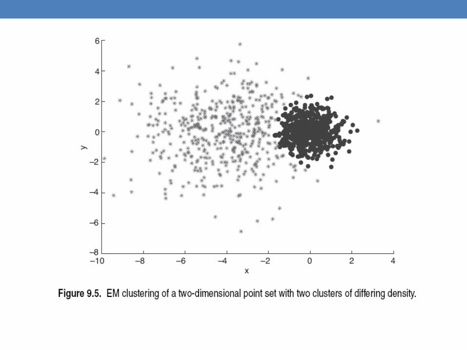
• Suppose that you have the heights of people from Greece and China and the distribution looks like the figure below (dramatization)

Mixture of Gaussians

• In this case the data is the result of the mixture of two Gaussians • One for Greek people, and one for Chinese people• Identifying for each value which Gaussian is most likely

to have generated it will give us a clustering.

Mixture model

• A value is generated according to the following process:• First select the nationality

• With probability select Greek, with probability select China

• Given the nationality, generate the point from the corresponding Gaussian• if Greece• if China

We can also thing of this as a Hidden Variable Z

• Our model has the following parameters

• For value , we have:

• For all values

• We want to estimate the parameters that maximize the Likelihood of the data

Mixture Model

Mixture probabilities Distribution Parameters

Mixture Models

• Once we have the parameters we can estimate the membership probabilities and for each point : • This is the probability that point belongs to the Greek or

the Chinese population (cluster)

EM (Expectation Maximization) Algorithm

• Initialize the values of the parameters in to some random values

• Repeat until convergence• E-Step: Given the parameters estimate the membership

probabilities and • M-Step: Compute the parameter values that (in expectation)

maximize the data likelihood

𝜇𝐶=∑𝑖=1

𝑛 𝑃 (𝐶|𝑥 𝑖 )𝑛∗𝜋𝐶

𝑥 𝑖

𝜋𝐶=1𝑛∑𝑖=1

𝑛

𝑃(𝐶∨𝑥 𝑖)𝜋𝐺=1𝑛∑𝑖=1

𝑛

𝑃 (𝐺∨𝑥𝑖)

𝜇𝐺=∑𝑖=1

𝑛 𝑃 (𝐺|𝑥𝑖 )𝑛∗𝜋𝐺

𝑥𝑖

𝜎𝐶2 =∑

𝑖=1

𝑛 𝑃 (𝐶|𝑥 𝑖 )𝑛∗𝜋𝐶

(𝑥𝑖−𝜇𝐶 )2 𝜎𝐺2 =∑

𝑖=1

𝑛 𝑃 (𝐺|𝑥𝑖 )𝑛∗𝜋𝐺

(𝑥 𝑖−𝜇𝐺 )2

MLE Estimatesif ’s were fixed

Fraction of population in G,C

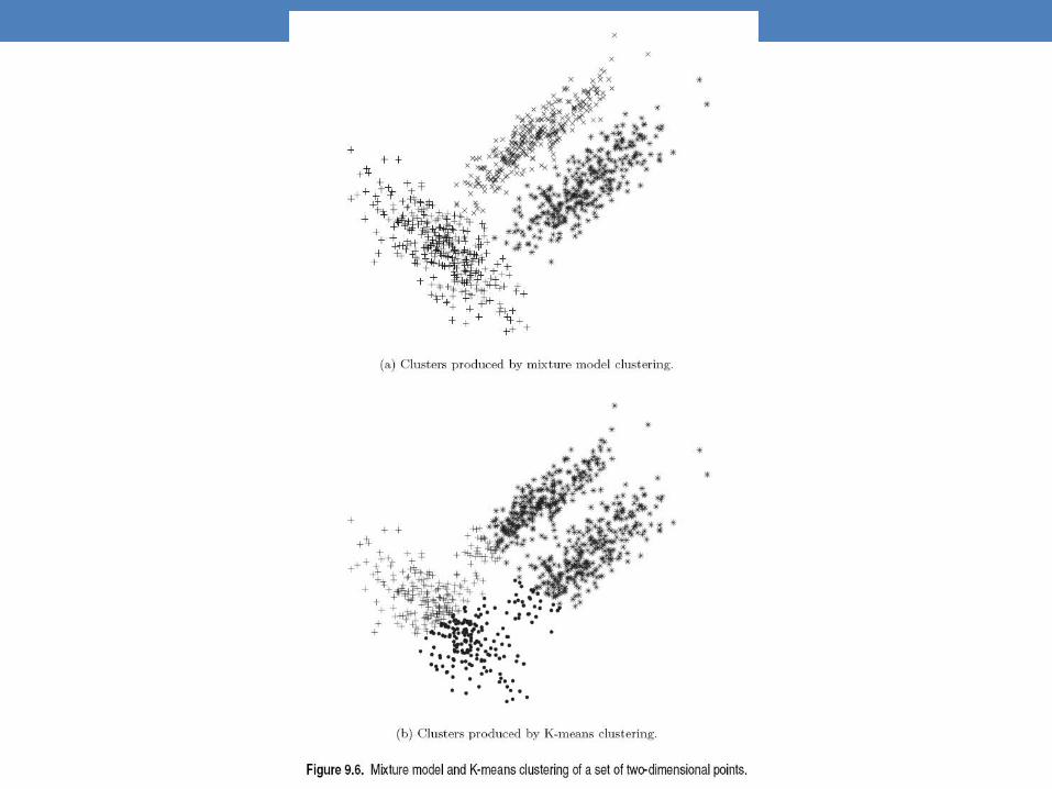
Relationship to K-means

• E-Step: Assignment of points to clusters • K-means: hard assignment, EM: soft assignment

• M-Step: Computation of centroids• K-means assumes common fixed variance (spherical

clusters)• EM: can change the variance for different clusters or

different dimensions (elipsoid clusters)

• If the variance is fixed then both minimize the same error function