Data Modeling and Least Squares Fitting

COS 323

Last time: Linear Systems Part 2

•  Iterative refinement

•  Fixed-point stationary methods –  Formulations for root-finding and linear systems –  Iterative refinement as a stationary method –  Iterative methods for large systems:

•  Jacobi, Gauss-Seidel, Successive Over-Relaxation

•  Sherman-Morrison: Rank-1 updating

•  Conjugate gradient (formulating a linear system as an optimization problem)

•  Representing sparse systems

Outline

•  What is data modeling and why do it?

•  Why choose a model that minimizes sum of squared error?

•  How to formulate and compute the optimal least-squares linear model?

•  Illustrating least-squares with special cases: constant, line

•  Weighted least squares

•  How to judge the quality of a model?

Data Modeling

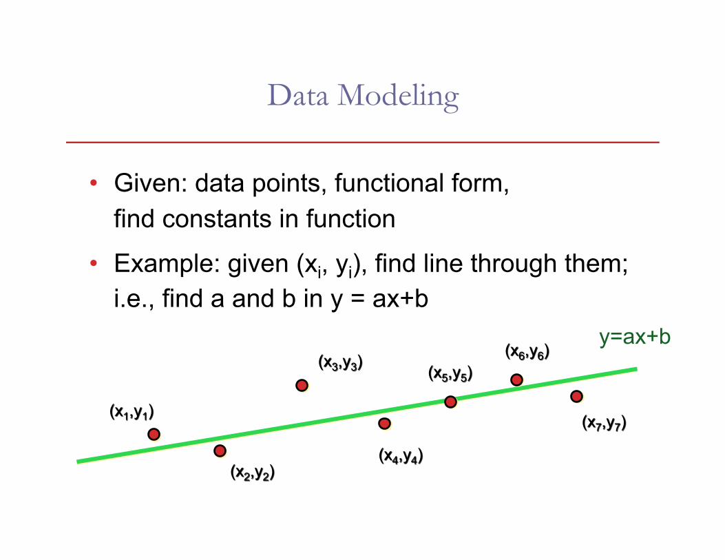
•  Given: data points, functional form, find constants in function

•  Example: given (xi, yi), find line through them; i.e., find a and b in y = ax+b

y=ax+b

Data Modeling

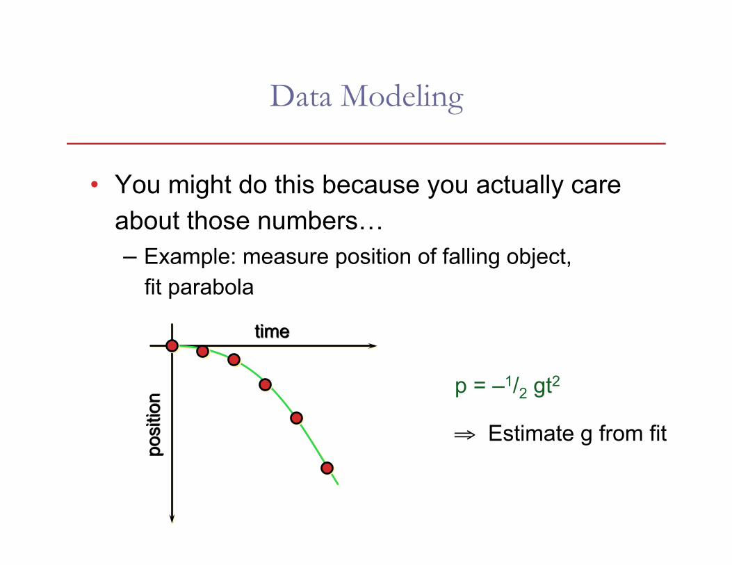
•  You might do this because you actually care about those numbers… – Example: measure position of falling object,

fit parabola

p = –1/2 gt2

⇒ Estimate g from fit

Data Modeling

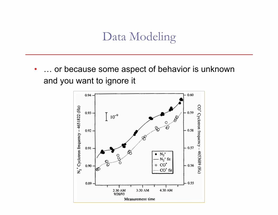
•  … or because some aspect of behavior is unknown and you want to ignore it

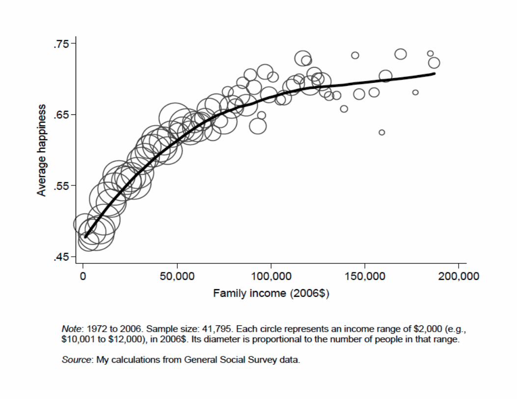
Historical context

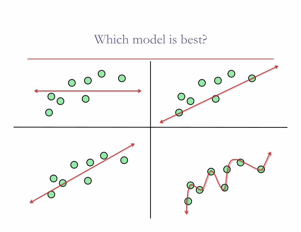
Which model is best?

Best-fit lines under different metrics

Least Squares

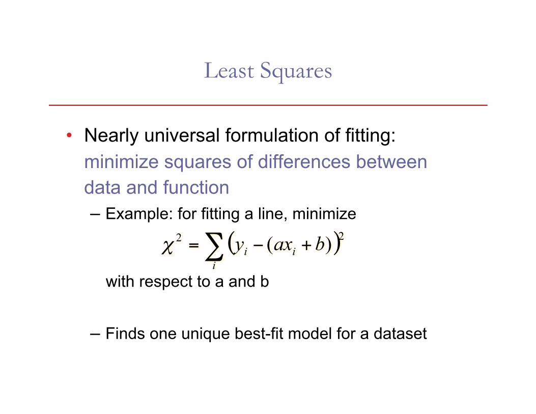
•  Nearly universal formulation of fitting: minimize squares of differences between data and function – Example: for fitting a line, minimize

with respect to a and b

– Finds one unique best-fit model for a dataset

Linear Least Squares

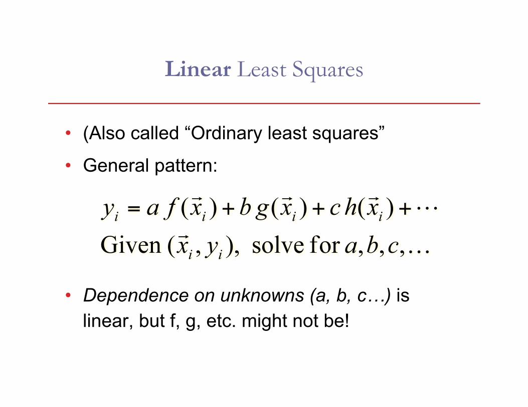
•  (Also called “Ordinary least squares”

•  General pattern:

•  Dependence on unknowns (a, b, c…) is linear, but f, g, etc. might not be!

Linear Least Squares Examples

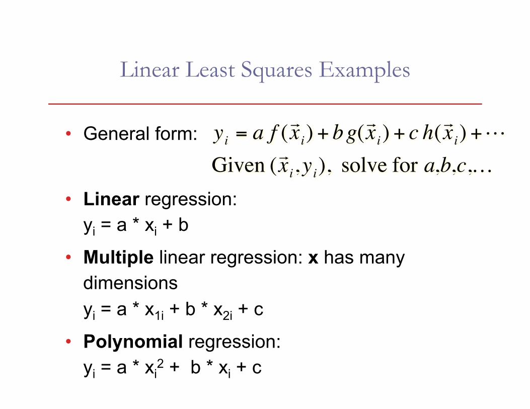
•  General form:

•  Linear regression: yi = a * xi + b

•  Multiple linear regression: x has many dimensions yi = a * x1i + b * x2i + c

•  Polynomial regression: yi = a * xi

2 + b * xi + c

€

yi = a f ( x i) + bg( x i) + c h( x i) +Given ( x i,yi), solve for a,b,c,…

How do we compute the model parameters?

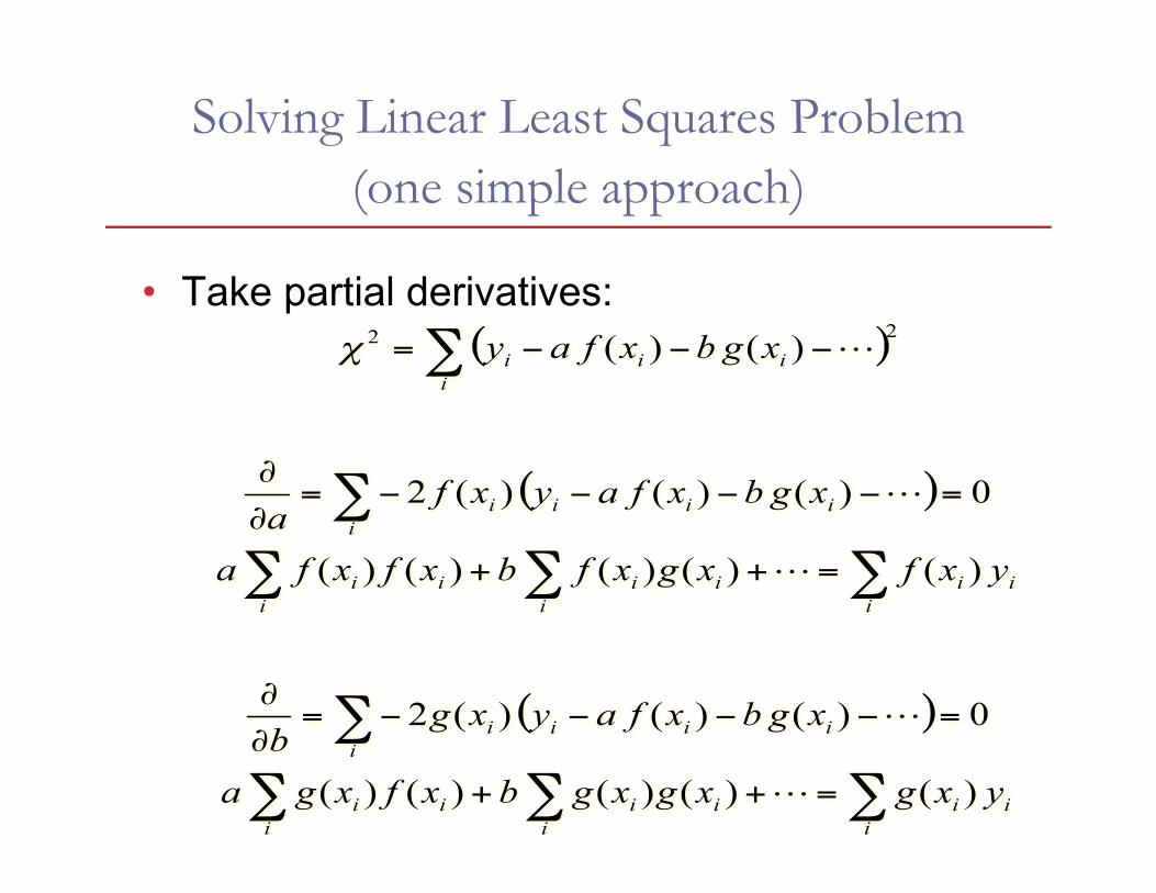
Solving Linear Least Squares Problem (one simple approach)

•  Take partial derivatives:

Solving Linear Least Squares Problem

•  For convenience, rewrite as matrix:

•  Factor:

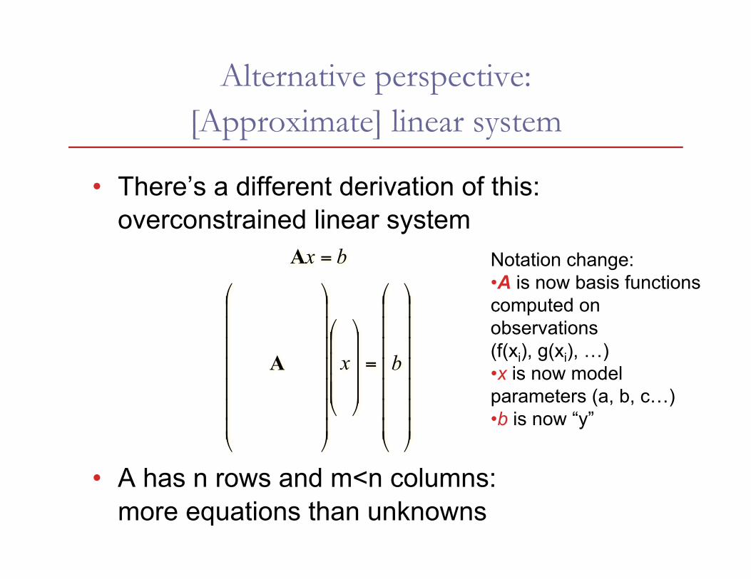
Alternative perspective: [Approximate] linear system

•  There’s a different derivation of this: overconstrained linear system

•  A has n rows and m<n columns: more equations than unknowns

Notation change: • A is now basis functions computed on observations (f(xi), g(xi), …) • x is now model parameters (a, b, c…) • b is now “y”

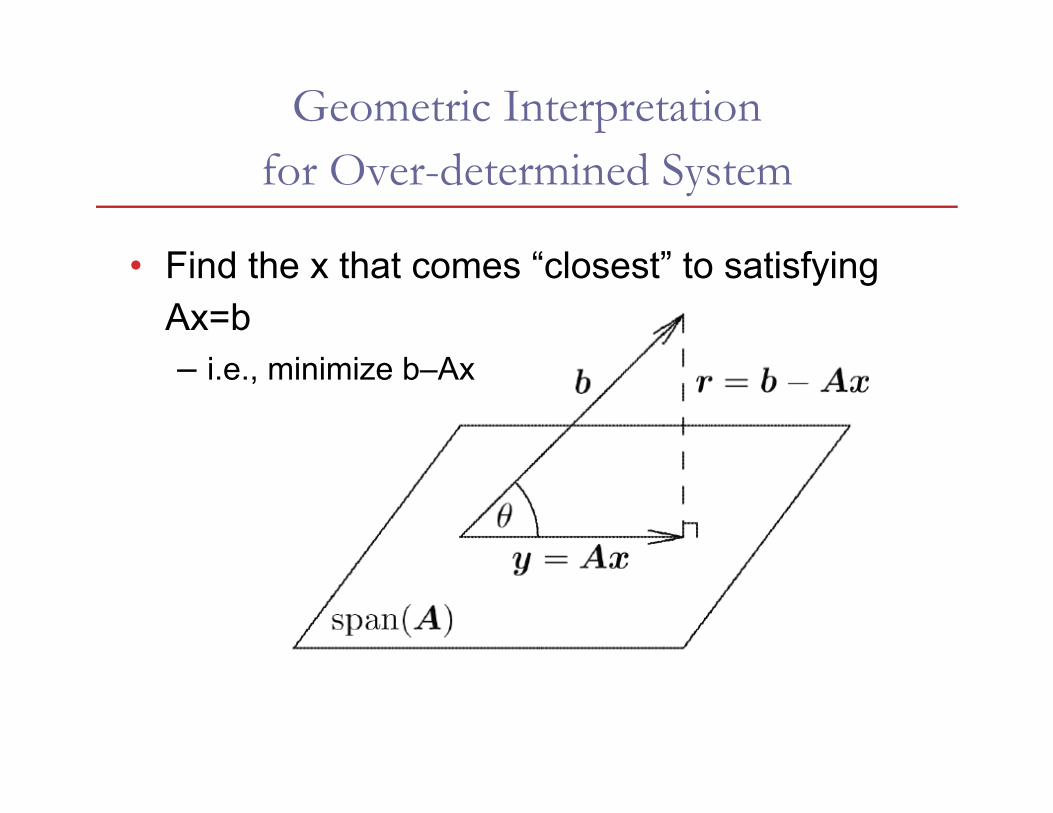
Geometric Interpretation for Over-determined System

•  Find the x that comes “closest” to satisfying Ax=b –  i.e., minimize b–Ax

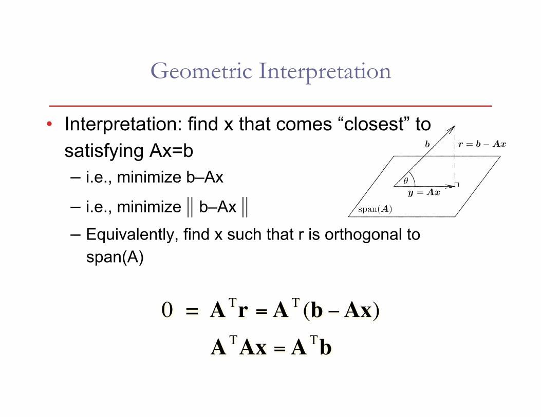
Geometric Interpretation

•  Interpretation: find x that comes “closest” to satisfying Ax=b –  i.e., minimize b–Ax

–  i.e., minimize || b–Ax ||

– Equivalently, find x such that r is orthogonal to span(A)

€

0 = A Tr =A T (b −Ax)A TAx =A Tb

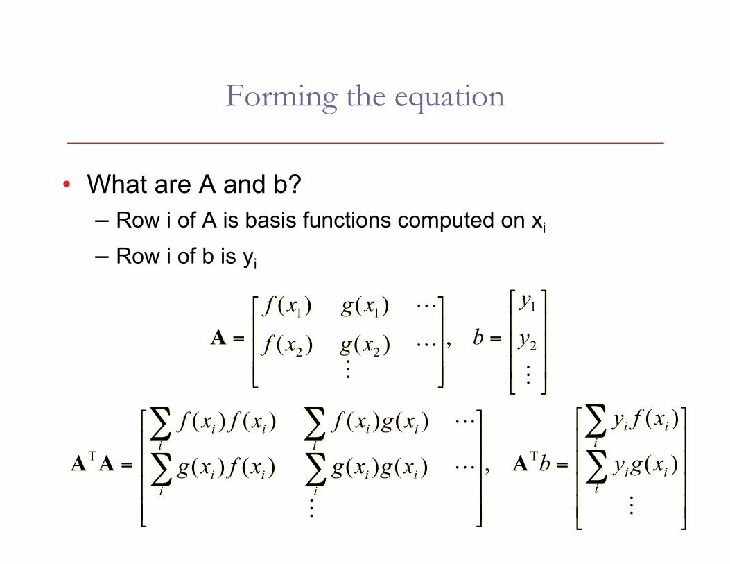
Forming the equation

•  What are A and b? – Row i of A is basis functions computed on xi – Row i of b is yi

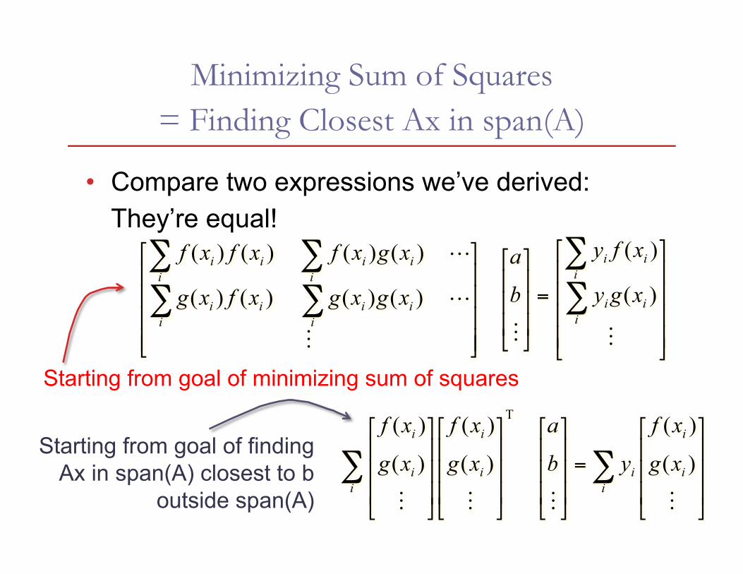
Minimizing Sum of Squares = Finding Closest Ax in span(A)

•  Compare two expressions we’ve derived: They’re equal!

Starting from goal of minimizing sum of squares

Starting from goal of finding Ax in span(A) closest to b

outside span(A)

Great, but how do we solve it?

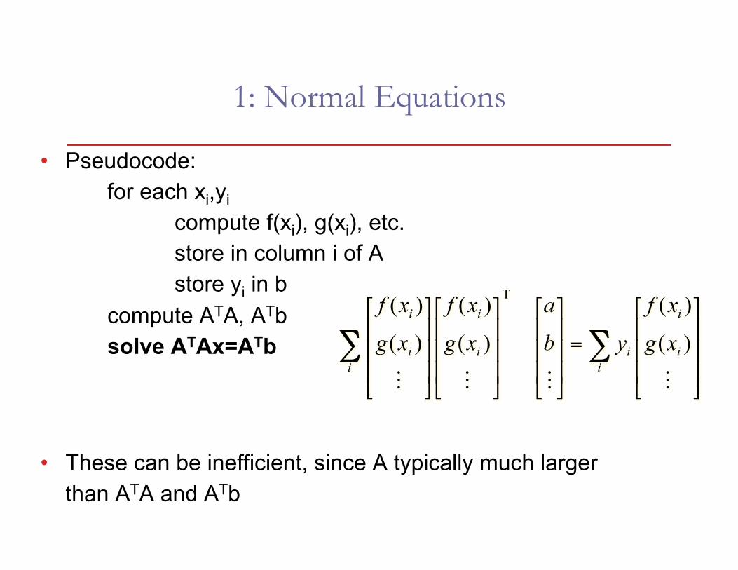
1: Normal Equations

•  Pseudocode: for each xi,yi

compute f(xi), g(xi), etc. store in column i of A store yi in b compute ATA, ATb solve ATAx=ATb

•  These can be inefficient, since A typically much larger than ATA and ATb

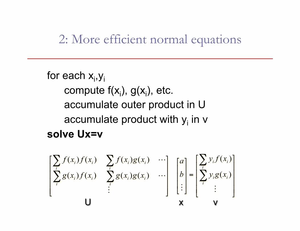
2: More efficient normal equations

for each xi,yi

compute f(xi), g(xi), etc. accumulate outer product in U accumulate product with yi in v

solve Ux=v

3: Using the pseudoinverse

for each xi,yi

compute f(xi), g(xi), etc. store in row i of A store yi in b

compute x = (ATA)-1 ATb

•  (ATA)-1 AT is known as “pseudoinverse” of A

The Problem with Normal Equations

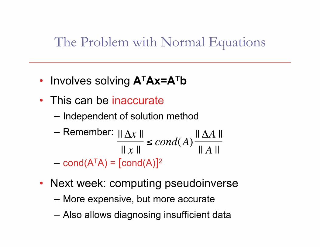
•  Involves solving ATAx=ATb

•  This can be inaccurate –  Independent of solution method – Remember:

–  cond(ATA) = [cond(A)]2

•  Next week: computing pseudoinverse – More expensive, but more accurate – Also allows diagnosing insufficient data

€

||Δx |||| x ||

≤ cond(A) ||ΔA |||| A ||

Special Cases

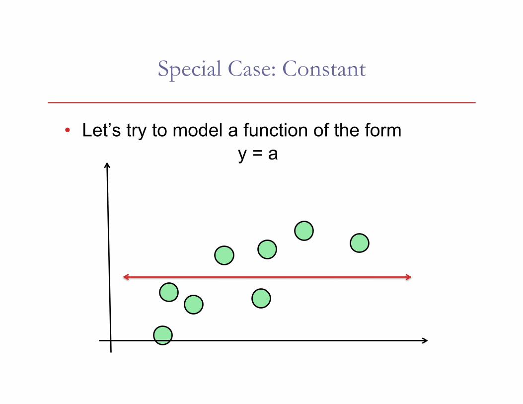
Special Case: Constant

•  Let’s try to model a function of the form y = a

Special Case: Constant

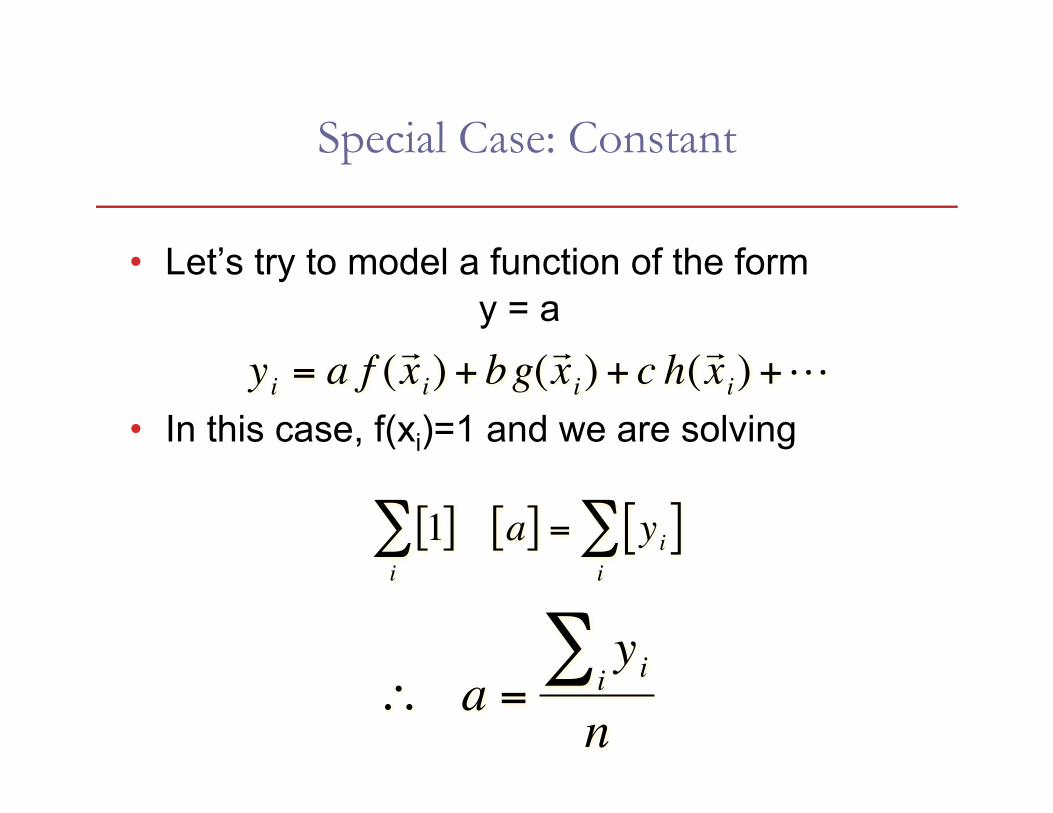
•  Let’s try to model a function of the form y = a

•  In this case, f(xi)=1 and we are solving

€

1[ ]i∑ a[ ] = yi[ ]

i∑

€

∴ a =yii

∑n

€

yi = a f ( x i) + bg( x i) + c h( x i) +

Special Case: Line

•  Fit to y=a+bx

•  f(xi)=1, g(xi)=x. So, solve:

Variant: Weighted Least Squares

Weighted Least Squares

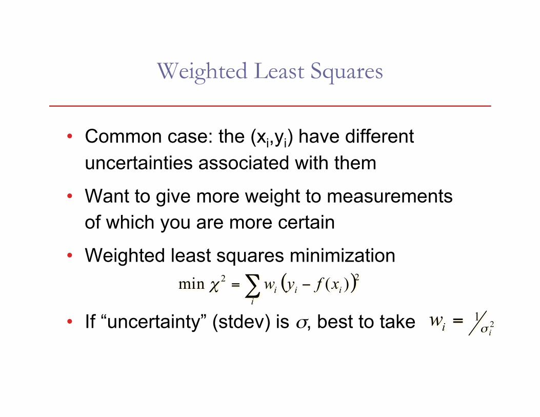
•  Common case: the (xi,yi) have different uncertainties associated with them

•  Want to give more weight to measurements of which you are more certain

•  Weighted least squares minimization

•  If “uncertainty” (stdev) is σ, best to take

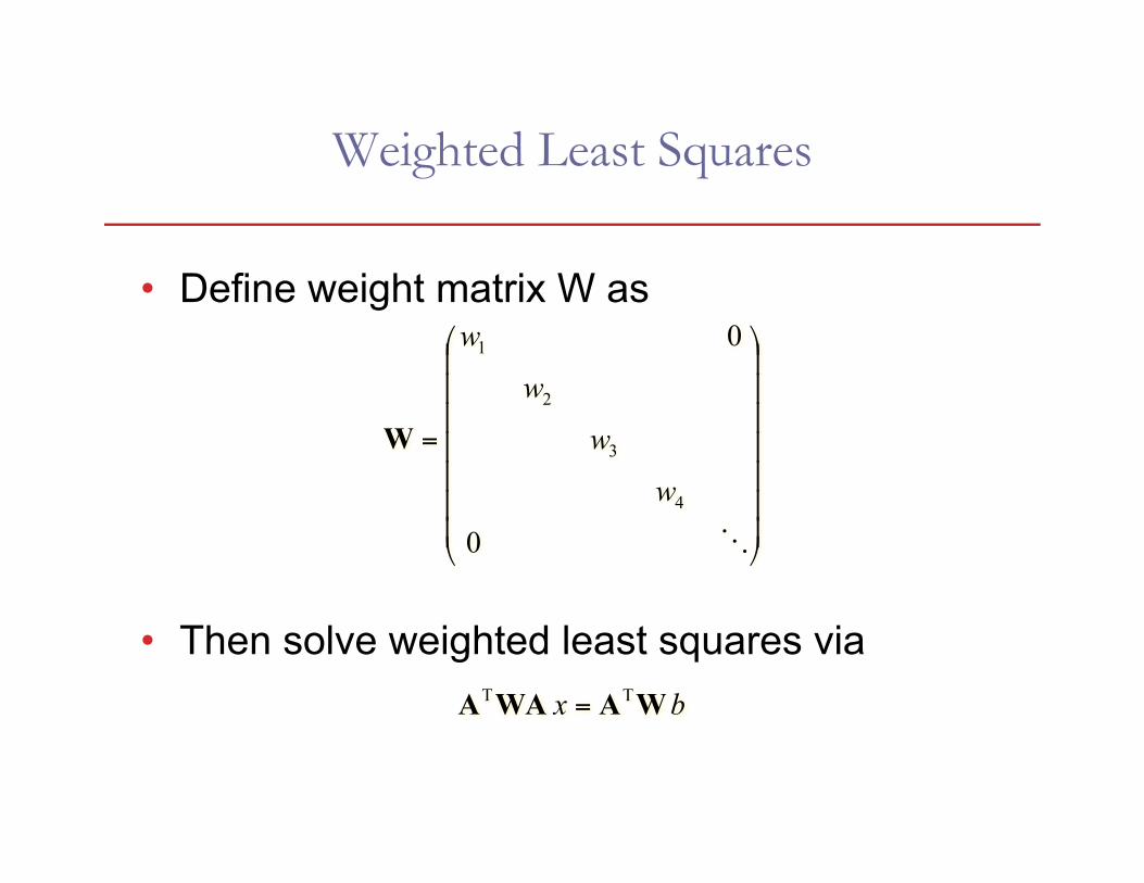
Weighted Least Squares

•  Define weight matrix W as

•  Then solve weighted least squares via

Understanding Error and Uncertainty

Error Estimates from Linear Least Squares

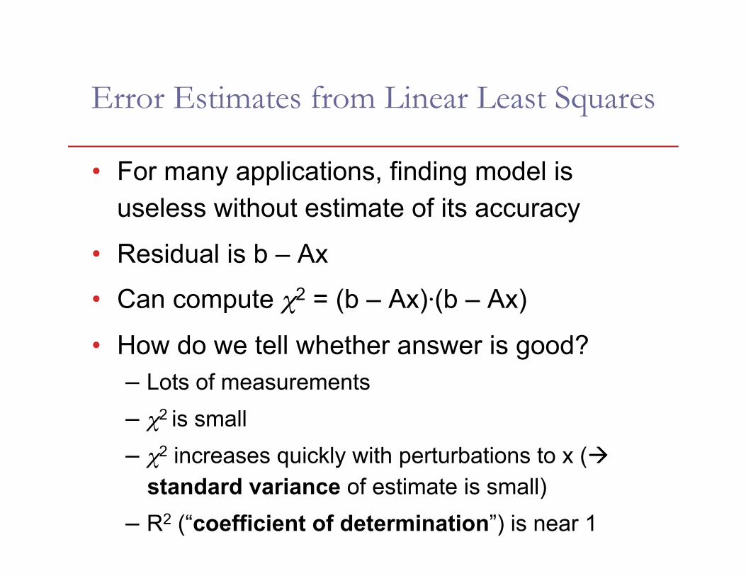
•  For many applications, finding model is useless without estimate of its accuracy

•  Residual is b – Ax

•  Can compute χ2 = (b – Ax)⋅(b – Ax)

•  How do we tell whether answer is good? –  Lots of measurements –  χ2

is small –  χ2 increases quickly with perturbations to x (

standard variance of estimate is small) – R2 (“coefficient of determination”) is near 1

Error Estimates from Linear Least Squares

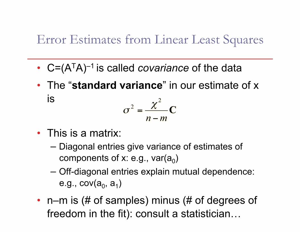
•  C=(ATA)–1 is called covariance of the data •  The “standard variance” in our estimate of x

is

•  This is a matrix: – Diagonal entries give variance of estimates of

components of x: e.g., var(a0) – Off-diagonal entries explain mutual dependence:

e.g., cov(a0, a1)

•  n–m is (# of samples) minus (# of degrees of freedom in the fit): consult a statistician…

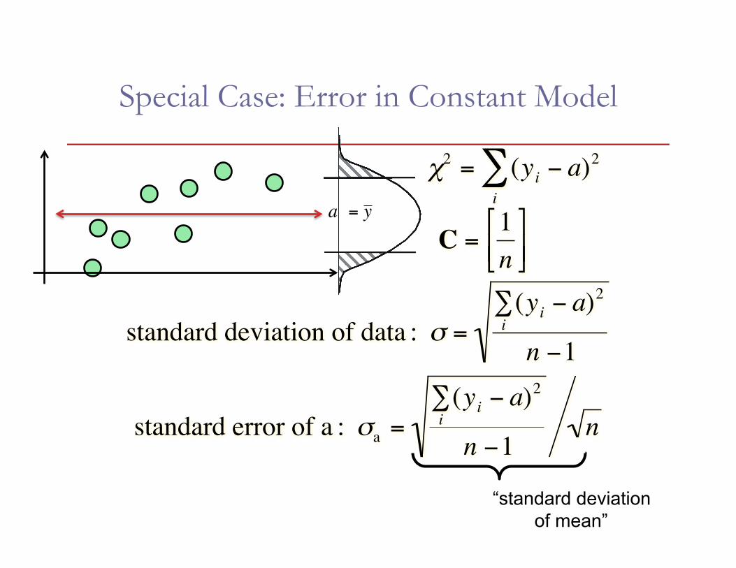
Special Case: Error in Constant Model

€

a = y

€

standard deviation of data : σ =(yi − a)2

i∑

n −1

standard error of a : σa =(yi − a)2

i∑

n −1n

€

χ2 = (yi − a)2

i∑

“standard deviation of mean”

€

C =1n⎡

⎣ ⎢ ⎤

⎦ ⎥

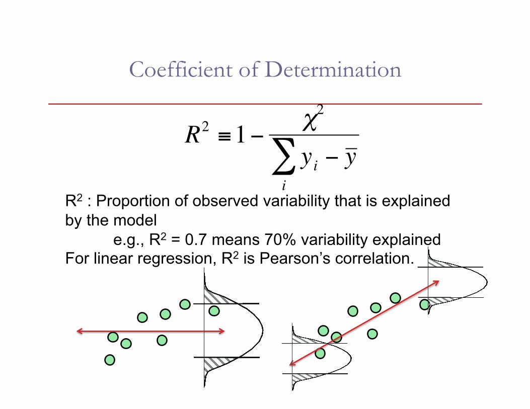
Coefficient of Determination

R2 : Proportion of observed variability that is explained by the model

e.g., R2 = 0.7 means 70% variability explained For linear regression, R2 is Pearson’s correlation.

€

R2 ≡1− χ2

yi − y i∑

Keep in mind…

•  In general, uncertainty in estimated parameters goes down slowly: like 1/sqrt(# samples)

•  Formulas for special cases (like fitting a line) are messy: simpler to think of ATAx=ATb form

•  Normal equations method often not numerically stable: orthogonal decomposition methods used instead

•  Linear least squares is not always the most appropriate modeling technique…

Next time

•  Non-linear models –  Including logistic regression

•  Dealing with outliers and bad data

•  Practical considerations –  Is least squares an appropriate method for my

data?

•  Examples with Excel and Matlab