1

School of Physics

Data Processing and Analysis Guide for Stage 6 Physics

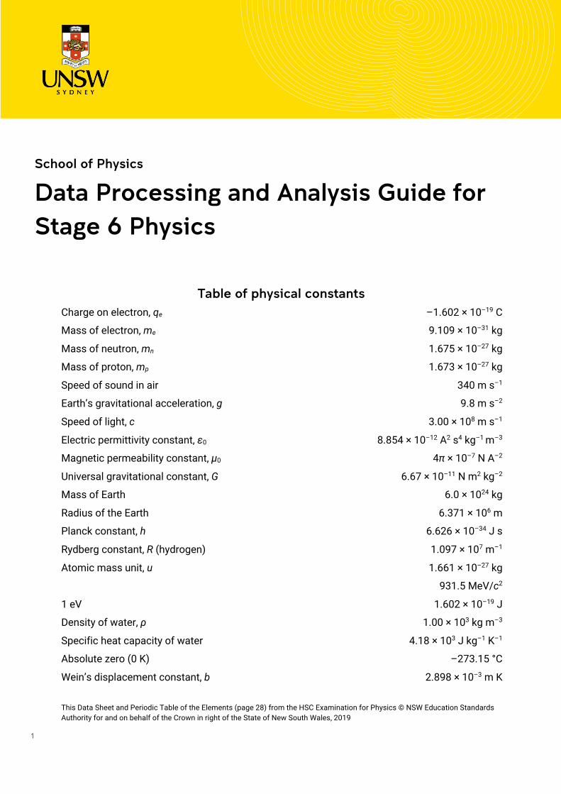
Table of physical constants Charge on electron, qe –1.602 × 10–19 C

Mass of electron, me 9.109 × 10–31 kg

Mass of neutron, mn 1.675 × 10–27 kg

Mass of proton, mp 1.673 × 10–27 kg

Speed of sound in air 340 m s–1

Earth’s gravitational acceleration, g 9.8 m s–2

Speed of light, c 3.00 × 108 m s–1

Electric permittivity constant, ε0 8.854 × 10–12 A2 s4 kg–1 m–3

Magnetic permeability constant, μ0 4π × 10–7 N A–2

Universal gravitational constant, G 6.67 × 10–11 N m2 kg–2

Mass of Earth 6.0 × 1024 kg

Radius of the Earth 6.371 × 106 m

Planck constant, h 6.626 × 10–34 J s

Rydberg constant, R (hydrogen) 1.097 × 107 m–1

Atomic mass unit, u 1.661 × 10–27 kg

931.5 MeV/c2

1 eV 1.602 × 10–19 J

Density of water, ρ 1.00 × 103 kg m–3

Specific heat capacity of water 4.18 × 103 J kg–1 K–1

Absolute zero (0 K) –273.15 °C

Wein’s displacement constant, b 2.898 × 10–3 m K

This Data Sheet and Periodic Table of the Elements (page 28) from the HSC Examination for Physics © NSW Education Standards Authority for and on behalf of the Crown in right of the State of New South Wales, 2019

2

Introduction

This guide is intended for teachers of the Stage 6 Physics course in New South Wales. It draws upon resources published by the NSW Department of Education in their Working Scientifically support documents as well as those from the School of Physics First Year Unit at the University of New South Wales, Sydney.

The definitions and procedures described in this guide take into consideration the differences between what is done in tertiary studies and research in physics, and the skills and understanding of students studying physics in high school.

It is intended to give teachers and their students a sense of good practice for processing and analysing data. It is in no way designed to be prescriptive; teachers should consider the learning requirements and outcomes for their students when using this guide.

References to the NSW Physics Stage 6 Syllabus PH11/12-4 Processing data and information A student selects and processes appropriate qualitative and quantitative data and information using a range of appropriate media.

Students:

• select qualitative and quantitative data and information and represent them using a range of formats, digital technologies and appropriate media (ACSPH004, ACSPH007, ACSPH064, ACSPH101)

• apply quantitative processes where appropriate • evaluate and improve the quality of data

PH11/12-5 Analysing data and information A student analyses and evaluates primary and secondary data and information

Students:

• derive trends, patterns and relationships in data and information • assess error, uncertainty and limitations in data (ACSPH004, ACSPH005, ACSPH033,

ACSPH099) • assess the relevance, accuracy, validity and reliability of primary and secondary data and

suggest improvements to investigations (ACSPH005)

Suggestions and corrections Please forward any suggestions or corrections by email to schools@phys.unsw.edu.au This edition published 2020 in the First Year Physics Unit School of Physics UNSW Sydney CRICOS Provider Code 00098G ©2020, University of New South Wales

3

Contents 1 – Recording data 4 1.1 Reporting data 4

1.1.1 Scientific notation and orders of magnitude 4 1.1.2 Significant figures 4 1.1.3 Units 5

1.2 Tabulating data 6 2 – Accuracy, errors and uncertainties 7 2.1 Error 7

2.1.1 Quantifying error 7 2.1.2 Using error to assess accuracy 7 2.1.3 Systematic and random errors 8 2.1.4 Improving accuracy – reducing errors 8

2.2 Uncertainty 9 2.2.1 Uncertainty versus error 9 2.2.2 Using uncertainty to assess accuracy 9 2.2.3 Reporting uncertainties 10 2.2.4 Uncertainty in values read directly from a measuring device 10 2.2.5 Uncertainties due to environmental or human factors 11 2.2.6 Uncertainty in the average from a series of repeated measurements 11 2.2.7 Uncertainty in the slope of a line of best fit 12 2.2.8 Reducing uncertainties 12 2.2.9 Combining uncertainties 13

3 – Reliability and validity 15 3.1 Reliability 15

3.1.1 Evaluating and assessing reliability 15 3.1.2 Addressing the causes of unreliability 15

3.2 Validity 16 3.2.1 Assessing validity 16 3.2.2 Examining data for the indicators of invalidity 16

4 – Analysing data 17 4.1 General principles 17 4.2 Linearized equations 18 4.3 Plotting graphs by hand 19

4.3.1 Drawing lines of best fit 19 5 – Using spreadsheets 21 5.1 Entering data 21 5.2 Performing calculations 21 5.3 Plotting a graph 23 5.4 Obtaining the uncertainty in the slope 25 5.5 Common spreadsheet symbols and functions 26

5.5.1 Calling on cells in functions 26 5.5.2 Order of operations 26 5.5.3 Entering data 26 5.5.4 Common functions 27

Exercises 28 Solutions to exercises 32 References 32

4

1 – Recording data

1.1 Reporting data

1.1.1 Scientific notation and orders of magnitude

A neat way of recording very large or very small numbers is by using scientific notation. This is where numbers are written as a product of powers of ten, also called orders of magnitude. For example:–

• 2 560 000 m can be written as 2.56 × 106 m

• 0.0000183 m can be written as 1.83 × 10–5 m

These numbers are 11 orders of magnitude apart, since there are 11 powers of ten between 106 and 10–5.

Note that numbers like 8.4 × 106 m have an order of magnitude of 7 because it rounds up to 107.

1.1.2 Significant figures

Significant figures are important because they signal the accuracy or uncertainty in a value. The last significant figure in a number suggests that it is accurate to ±½ of its place. For example, 5.3 km implies a distance with uncertainty of 5.30 ± 0.05 km but 5.34 km implies 5.340 ± 0.005 km.

Rules for significant figures – what counts as a significant figure?

• Non-zero digits are significant. • Trailing zeroes in a whole number are generally not significant (these zeroes are used to keep the

other figures in their correct value places). ‒ 75000 m – the 7 and 5 are significant. There are 2 significant figures. ‒ 75420 m – the 7, 5, 4 and 2 are significant. There are 4 significant figures. There is less

uncertainty in this number. • Sometimes trailing zeroes are significant. They may be marked with an overbar or underlined.

‒ 5320"0 – 5, 3, 2 and one of the zeroes are significant. There are 4 significant figures. • Leading zeroes are not significant (these zeroes are used to keep the other figures in their correct

value places). ‒ 0.000832 kg – only 8, 3, and 2 are significant. There are 3 significant figures.

• The zeroes between non-zero digits are significant. ‒ 90.04 s – each figure is significant. There are 4 significant figures.

• The trailing zeroes in a decimal are significant. ‒ 8.30 L – each figure is significant. There are 3 significant figures. ‒ 3.200 J – each figure is significant. There are 4 significant figures.

The result of a calculation is only as accurate as the least accurate value used to compute it. So, when reporting the result of a calculation, the result must be rounded to the same as the smallest number of significant figures of any value used in the calculation. For example,

Energy = 3.457 W × 5.60 s = 19.3292 J

the answer can only be reported as 19.3 J because the smallest number of significant figures in the calculation was three.

5

Note: In calculations consisting of simple additions and subtractions only, answers should be given with the same number of decimal places as the term with the least number of decimal places in the calculation. For example:

ΔT = 137.45 °C – 37.8766 °C = 99.5734 °C

The accuracy implied by the additional decimal places in one of the numbers is meaningless if the other number is more uncertain.

1.1.3 Units

Units add important information to measurements because a numerical value means nothing on its own.

A unit has to be an agreed quantity of a thing to be measured, because when we say or write down a measurement, we are actually giving a number of multiples of that unit. For example, when you are told that the length of something is 3 metres, you are being told that its length is 3 × 1 metre, and this will only be accurate if everyone agrees about what a single metre is.

The agreed system of units used in science is the International System of units (SI units). The base units are:

• Time – seconds (s) • Length – metres (m) • Mass – kilograms (kg) • Electric current – amperes (A)

• Thermodynamic temperature – kelvin (K) • Amount of substance – mole (mol) • Luminous intensity – candela (cd)

Some units are derived from the SI base units. Derived units can be determined from the equations used to calculate its quantity—they follow the usual rules for multiplication and division. For example, the units of speed are derived from the units for length and time (metres per second):

speed =distancetime

=1m1s

= 1m/s = 1m ∙ s!"

Some quantities are so special that their derived unit is given a name. For example, you might know the named unit for force – the newton (N). The unit for force is actually derived from the SI base units. Since force is determined by the equation

𝐹 = 𝑚𝑎

the unit for force derived from base units is

1newton = 1kg × 1m ∙ s!# = 1kg ∙ m ∙ s!#

Some other examples are:

Quantity Derived unit in terms of base units Named unit and symbol

Energy kg ∙ m# ∙ s!# joule (J)

Electric charge A ∙ s coulomb (C)

Frequency s!" hertz (Hz)

Pressure kg ∙ m!" ∙ s!# pascal (Pa)

Voltage kg ∙ m# ∙ s!$ ∙ A!" volt (V)

6

Prefixes are sometimes used to convert units into forms that are more conveniently written or spoken. Some examples (and their multipliers, in scientific notation):–

Prefix Symbol Multiplier Example

nano– n ×10–9 nanometre (nm)

micro– µ ×10–6 microampere (µA)

milli– m ×10–3 millivolt (mV)

centi– c ×10–2 centigram (cg)

deci– d ×10–1 decilitre (dL)

deca– da ×101 decade

hecto– h ×102 hectopascal (hPa)

kilo– k ×103 kilometre (km)

mega– M ×106 megajoule (MJ)

giga– G ×109 gigawatt (GW)

1.2 Tabulating data

Data should be recorded clearly in a table. Additional columns should be added for any processed data.

Best practice for a table in Stage 6 Physics should include:

• a descriptive title or caption • columns that have headings that include units, where appropriate; units are not included in the body

of the table • the independent variable, usually towards the left, and the dependent variable, towards the right • figures aligned by decimal point • uncertainties, if appropriate.

Example:

Table: the variation in the period of a pendulum as its length increases

Ten Periods, 10T (s)

Length (m) Trial 1 Trial 2 Trial 3 Average ± Uncertainty T2 (s2)

0.50 14.34 14.30 14.53 14.39 0.11 2.07

0.60 16.35 15.93 16.23 16.17 0.21 2.61

0.70 17.23 17.04 17.74 17.33 0.35 3.00

0.80 19.63 19.41 19.24 19.43 0.20 3.77

0.90 20.47 20.73 20.19 20.47 0.27 4.19

1.00 21.20 20.33 22.01 21.78 0.84 4.49

7

2 – Accuracy, errors and uncertainties

2.1 Error

2.1.1 Quantifying error

Accuracy is the closeness of an observed value to its “true” value (a true value could be some theoretical value, or a value accepted by physicists and tabulated in secondary sources).

On some level, every measurement is an approximation. One reason is that there are limitations in the instruments we use for measuring – they may lack sensitivity, or the graduations on them (their resolution) might not be fine enough.

Environmental factors can also interfere with making measurements, and we as humans have our limitations in making and reading measurements, too.

The difference between an observed value and its true value is called error (for us, it does not mean “mistake”, as is its common meaning).

The following equations can be used to quantify error and accuracy:

Absolute error |truevalue − observedvalue|

Relative error (also called percentage error when expressed as %)

|truevalue − observedvalue|truevalue

Accuracy 100%− percentageerror

For example, the “true” value of gravitational field strength on Earth’s surface is 9.8 N kg–1. In an experiment carried out by a student, the value observed was 8.5 N kg–1.

Absoluteerror = |9.8Nkg!" − 8.5Nkg!"| = 1.3Nkg!"

Relativeerror =|9.8Nkg!" − 8.5Nkg!"|

9.8Nkg!"= 13%

Accuracy = 100%− 13% = 87%

2.1.2 Using error to assess accuracy

An arbitrary limit can be set as a benchmark for accuracy, for example, 5% or 10% error.

An alternative might be to set “error bands” for a graduated scale of accuracy. For example, 0-5% for high accuracy, 5-15% error for modest accuracy, >15% for low accuracy.

8

2.1.3 Systematic and random errors

When you make multiple measurements and compute the errors, you might start to recognise patterns in how and when they occur. Because of this, errors can be put into one of two categories depending on how they behave:

• Systematic errors –When repeated, observed values are displaced in same direction from the true value. That is, the observed values might read consistently higher or consistently lower than the true value. These types of errors are often caused by improperly calibrated measuring instruments, or “zero” errors (such as when an electronic balance shows a non-zero reading when there is nothing on its pan – every reading will be higher than it should be).

• Random errors – When repeated, observed values are scattered randomly above and below the true value. These types of errors are often caused by random fluctuations in the ambient conditions or uncontrolled variables.

Systematic errors shift all measurements in the same direction.

Random errors cause measurements to spread randomly in all directions.

2.1.4 Improving accuracy – reducing errors

To increase accuracy, we need to reduce error. We can do that by modifying experimental techniques or procedures to make the error absolutely smaller, or by making the error smaller relative to the value we are measuring. Here are some ways to reduce error:

• To reduce absolute error ‒ Use measuring instruments with appropriate resolution (graduations fine enough for the quantity

you are measuring). ‒ Read analogue instruments directly front-on to reduce parallax.

• To reduce relative error ‒ Design experiments to increase the size of measurements being made. For example, if we were to

measure the swinging time of a short pendulum, it might have a period of about 1.0 seconds; timing error with a stopwatch might be 0.5 seconds, so relative error is »0.5/1.0 = 50%. A longer pendulum’s period might be 10.0 seconds, so the relative error is »0.5/10.0 = 5%.

• To reduce systematic error ‒ Ensure that measuring instruments are properly calibrated and zeroed.

• To reduce random error ‒ Hold controlled variables constant (such as keeping ambient conditions stable) so that they do not

add fluctuations to a set of trials. ‒ Conduct repeated trials of a measurement and compute an average. (An average seeks to find the

centre of a set of values – remember that random error causes data to scatter randomly around the true value.)

9

2.2 Uncertainty

2.2.1 Uncertainty versus error

While the concept of error compares measurements against values assumed to be “true”, there are many more values (particularly direct measurements) that cannot be compared to known or accepted values.

Additionally, it is possible that a result close to an accepted value comes about purely by chance anyway. Calculating the error in cases like this does not tell us about the confidence we should have in the techniques used to make the measurement.

What we should also do is report our measurements with some indication of the certainty we have in it.

Remember, every measurement we make is, on some level, an approximation. To communicate how precise we think our measurement is, we can cite the possible margin of error which we call uncertainty.

How do we know how big the uncertainty in our measurements are? In sections 2.2.3–2.2.7, we discuss how to estimate uncertainties.

2.2.2 Using uncertainty to assess the quality of a value

A measurement agrees with an accepted value if the accepted value falls within the measurement’s uncertainty bounds. For example, when comparing the generally accepted value of acceleration due to gravity at Earth’s surface (g = 9.8 m.s–2), a measurement of:

• 9.6 ± 0.3 m.s–2 agrees, because 9.8 m.s–2 lies inside the range of 9.3 and 9.9 m.s–2 • 9.2 ± 0.3 m.s–2 does not agree, because 9.8 m.s–2 lies outside the range of 8.9 and 9.5 m.s–2

8.0 9.0 10.0 (m.s–2)

The arrows point to values on the number line and the grey bars are the uncertainty ranges. Only one of the measurements includes the accepted value.

Of course, you can make an accepted value can fall inside any uncertainty bounds if you make the uncertainty large enough. So for the measurement to be precise, the uncertainties also have to be reasonably small.

Approximate length, L

g = 9.8 m.s –2

agrees 9.6 ± 0.3

9.2 ± 0.3 disagrees

Uncertainty –ΔL +ΔL

10

2.2.3 Reporting uncertainties

Any value that has been observed or estimated has an associated uncertainty. Values that have been recorded should be quoted with an associated uncertainty.

Absolute uncertainty is expressed in the same dimensions as the value. For example, 5.4 ± 0.2 m could be a length where the true value might lie 0.2 m above or below the estimation of 5.4 m.

Relative uncertainty is the size of the uncertainty as a fraction of the observed or estimated value and is usually presented as a percentage.

Absolute uncertainty (has the same units as the measurement) Δ𝑥

Relative uncertainty (also called percentage uncertainty when expressed as %)

Δ𝑥𝑥

For example, for the estimation 5.4 ± 0.2 m, the relative uncertainty is %.#'.(= 4%

Uncertainty should be given to one significant figure*; the observed or estimated value should be rounded to same number of decimal places as the uncertainty (any more decimal places than the uncertainty would be meaningless).

For example, the height of a building might be 14.7 ± 0.5 m, not 14.691 ± 0.53 m.

* If the first significant figure of the uncertainty is a “1”, then a second significant figure is sometimes given. The number of decimal places must still match. For example, 12.67 ± 0.12 m.

2.2.4 Uncertainty in values read directly from a measuring device The minimum uncertainty in an observation made directly from a measuring device is equal to half of the smallest readable graduation on the scale of the device:

Uncertainty due to measuring instrument ±12× (instrumentgraduation)

Analogue devices

This ammeter has graduations in milliamperes. Any observation made with this device will have an uncertainty of ±0.5 mA.

Digital devices

This digital multimeter in 20VDC mode measures in increments of 0.01 V. Any observation made with this device in this mode will have an uncertainty of ±0.005 V.

11

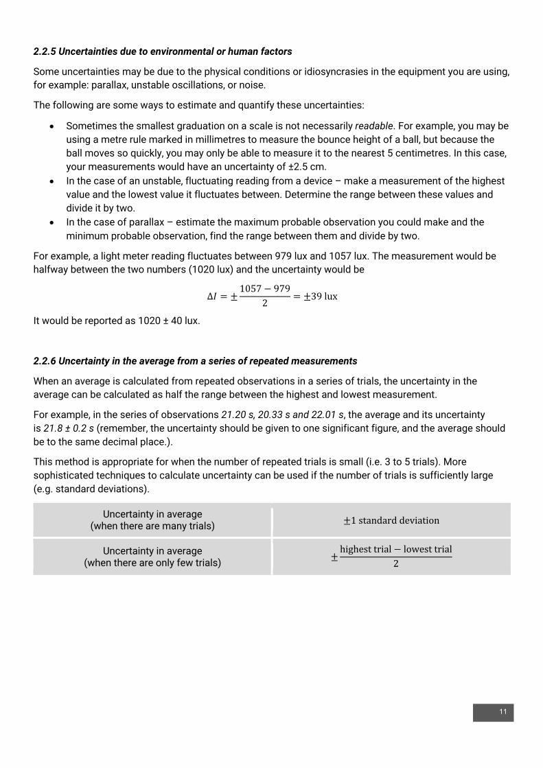
2.2.5 Uncertainties due to environmental or human factors

Some uncertainties may be due to the physical conditions or idiosyncrasies in the equipment you are using, for example: parallax, unstable oscillations, or noise.

The following are some ways to estimate and quantify these uncertainties:

• Sometimes the smallest graduation on a scale is not necessarily readable. For example, you may be using a metre rule marked in millimetres to measure the bounce height of a ball, but because the ball moves so quickly, you may only be able to measure it to the nearest 5 centimetres. In this case, your measurements would have an uncertainty of ±2.5 cm.

• In the case of an unstable, fluctuating reading from a device – make a measurement of the highest value and the lowest value it fluctuates between. Determine the range between these values and divide it by two.

• In the case of parallax – estimate the maximum probable observation you could make and the minimum probable observation, find the range between them and divide by two.

For example, a light meter reading fluctuates between 979 lux and 1057 lux. The measurement would be halfway between the two numbers (1020 lux) and the uncertainty would be

∆𝐼 = ±1057 − 979

2= ±39lux

It would be reported as 1020 ± 40 lux.

2.2.6 Uncertainty in the average from a series of repeated measurements

When an average is calculated from repeated observations in a series of trials, the uncertainty in the average can be calculated as half the range between the highest and lowest measurement.

For example, in the series of observations 21.20 s, 20.33 s and 22.01 s, the average and its uncertainty is 21.8 ± 0.2 s (remember, the uncertainty should be given to one significant figure, and the average should be to the same decimal place.).

This method is appropriate for when the number of repeated trials is small (i.e. 3 to 5 trials). More sophisticated techniques to calculate uncertainty can be used if the number of trials is sufficiently large (e.g. standard deviations).

Uncertainty in average (when there are many trials) ±1standarddeviation

Uncertainty in average (when there are only few trials) ±

highesttrial − lowesttrial2

12

2.2.7 Uncertainty in the slope of a line of best fit There is uncertainty associated with the gradient of a line of best fit (LOBF).

To estimate its uncertainty, the data points should be plotted with their respective error bars (the length of an error bar is the uncertainty in each data point).

Two lines of worst fit (LOWF) should then be drawn. One line of worst fit is the shallowest straight line that can be drawn yet passing through the error bars of as many data points as possible. Similarly, the other line of worst fit is the steepest straight line that can be drawn.

The uncertainty in the gradient of a line of best fit is then half of the difference between the gradients of the maximum and minimum lines of worst fit.

Uncertainty in line of best fit (LOBF) gradient ±maxLOWFgradient − min LOWFfit gradient

2

If a value of interest is extracted from the gradient using mathematical operations, then the value’s uncertainty can be determined using the method for when uncertain values are multiplied or divided (see 2.2.9 Combining uncertainties – when values are multiplied or divided).

Usually, the relative uncertainty in the LOBF gradient is the same as the relative uncertainty in the value of interest that you are extracting from it.

∆𝑎𝑎=∆LOBFgradientLOBFgradient

For example, if we are to use the data from a pendulum’s T2 vs l graph to determine the acceleration due to

gravity g, we can infer that 𝑔 = ()!

*+,-/0123456 (see 4.2 Linearized equations). Note how we have conducted a

division operation here.

Since 4 is an integer and π is a constant, they do not have uncertainties. Thus the relative uncertainty in g is

∆𝑔𝑔=∆LOBFgradientLOBFgradient

If the other values in the term that we have equated with the gradient had uncertainties, then we would just add their relative uncertainties, as in section 2.2.9.

2.2.8 Reducing uncertainties

Uncertainties can be reduced in the same ways that we have discussed when reducing errors (see 2.1.4 Improving accuracy – reducing errors).

13

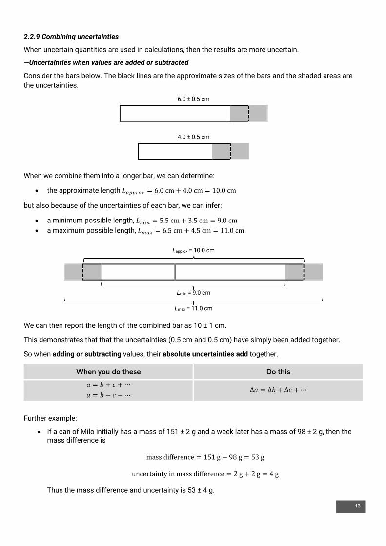
2.2.9 Combining uncertainties

When uncertain quantities are used in calculations, then the results are more uncertain.

—Uncertainties when values are added or subtracted

Consider the bars below. The black lines are the approximate sizes of the bars and the shaded areas are the uncertainties.

6.0 ± 0.5 cm

4.0 ± 0.5 cm

When we combine them into a longer bar, we can determine:

• the approximate length 𝐿7889:; = 6.0cm + 4.0cm = 10.0cm

but also because of the uncertainties of each bar, we can infer:

• a minimum possible length, 𝐿<=> = 5.5cm + 3.5cm = 9.0cm • a maximum possible length, 𝐿<7; = 6.5cm + 4.5cm = 11.0cm

We can then report the length of the combined bar as 10 ± 1 cm.

This demonstrates that that the uncertainties (0.5 cm and 0.5 cm) have simply been added together.

So when adding or subtracting values, their absolute uncertainties add together.

When you do these Do this

𝑎 = 𝑏 + 𝑐 +⋯ 𝑎 = 𝑏 − 𝑐 −⋯

∆𝑎 = ∆𝑏 + ∆𝑐 +⋯

Further example:

• If a can of Milo initially has a mass of 151 ± 2 g and a week later has a mass of 98 ± 2 g, then the mass difference is

massdifference = 151g − 98g = 53g

uncertaintyinmassdifference = 2g + 2g = 4g Thus the mass difference and uncertainty is 53 ± 4 g.

Lapprox = 10.0 cm

Lmin = 9.0 cm

Lmax = 11.0 cm

14

—Uncertainties when values are multiplied or divided Consider the rectangle below. The black line is the approximate size of the rectangle and the shaded area is the uncertainty.

We can multiply the approximate lengths of the sides to determine: • the approximate area of the rectangle, 𝐴7889:; = 6cm × 4cm = 24cm#

but because of the uncertainties, we can infer: • a minimum possible area, 𝐴<=> = 5.5cm × 3.5cm = 19cm# • a maximum possible area, 𝐴<7; = 6.5cm × 4.5cm = 29cm#

So we can report the area of the rectangle as 24 ± 5 cm2.

It’s a bit harder to see here, but when you multiply or divide values, their relative uncertainties add together to give the relative uncertainty in the result.

When you do these Do this

𝑎 = 𝑏 × 𝑐 ×⋯ 𝑎 = 𝑏 ÷ 𝑐 ÷⋯

∆𝑎𝑎=∆𝑏𝑏+∆𝑐𝑐+⋯

Let’s try this for the uncertainty for our rectangle example.

∆𝐴𝐴=∆𝐿𝐿+∆𝑊𝑊

→ ∆𝐴 = 𝐴g∆𝐿𝐿+∆𝑊𝑊 h = 24cm# g

0.56.0

+0.54.0h

= 5cm#

which is what we found geometrically.

Further example (uncertainty in a squared value):

• Given that the period of a pendulum T = 2.35 ± 0.03 s, then T2 (=T×T) and its uncertainty:

𝑇# = (2.35s)# = 5.52s#

∆𝑇#

𝑇#=∆𝑇𝑇+∆𝑇𝑇→ ∆𝑇# = 𝑇# g

∆𝑇𝑇+∆𝑇𝑇 h

= 5.52s# g0.032.35

+0.032.35h

= 0.14s#

Thus T2 = 5.5 ± 0.1 s2

L = 6.0 ± 0.5 cm

W =

4.0

± 0

.5 c

m

15

3 – Reliability and validity

3.1 Reliability

Reliability refers to the consistency in results – repetition returns results that lie within a small margin of error. There are two ways of looking at reliability:

• Internal reliability is when repeated trials within an experiment are consistent. This is sometimes also called precision.

• External reliability is when the results from one experiment are consistent with those from other experiments that are conducted the same way.

When assessing reliability, sometimes it is enough to make broad subjective judgements (for example, “overall, the results appear to be roughly consistent”) but it is preferable to fall back on some kind of quantitative basis.

3.1.1 Evaluating and assessing reliability

One way to assess reliability might be to quantify the spread of trials around an average – large spreads are unreliable, and smaller spreads are reliable.

Data from reliable trials are clustered closely.

Data from unreliable trials are much more spread out.

We could judge a set of trials to be reliable if the relative uncertainty of the trials is less than some arbitrary limit, say, less than 5%.

For example, the following measurements of the same resistor were collected. The average is shown and the uncertainty was calculated (cf. §2.2.6 – Uncertainty in the average from a series of repeated measurements):

Trial 1 Trial 2 Trial 3 Average and uncertainty

94.8 Ω 106.3 Ω 100.2 Ω 100 ± 6 Ω

The relative uncertainty of this data set is ?@"%%@

or 6%. According to our arbitrary criteria, these trials are not reliable. Perhaps it might be better to say that they have low reliability.

3.1.2 Addressing the causes of unreliability

The opposite of reliability can be said to be variability. Recall that random errors cause repeated observations to vary randomly, so reducing the effects of random errors are a way to improve reliability.

Note that simply repeating trials or experiments on their own does not improve reliability. Repetition can help to assess reliability, but unless the underlying causes are addressed, then repetition may only continue displaying variability.

16

3.2 Validity

A valid experiment is one that examines what is intended – the relationship between an independent variable and a dependent variable. There must be minimal interference in this relationship by other factors – these other factors might be the variables that we should control (hold constant), or the level of care with which we conduct the experiment and make measurements.

If we only vary the independent variable and keep all the other variables the same, then we can be confident that the effects that we observe are due only to the changes that we have made. We can say that the experiment is valid.

However, if we do not keep the other variables the same, then we cannot be certain that our observations are only due to the independent variable. This would mean that the experiment would be invalid.

If we are careless when we conduct experiments, make inaccurate measurements, or use inappropriate equipment, then his also invalidates the experiment.

3.2.1 Assessing validity

Remember that you should only vary the independent variable and make observations of the dependent variable.

Then you have to ask: have all the other variables been held constant?

• If yes, then you can be confident that the experiment and its results are valid. • If no, then there are doubts about the validity of the experiment and its results.

3.2.2 Examining the data for indicators of invalidity

It might be difficult to account for absolutely all the variables that are present in the space where you are conducting your experiment. So we can look to the data to see if we have allowed any variables to go uncontrolled:

Unreliability in data

Uncontrolled variables can cause variability in repeated measurements.

Unreliable results → invalid experiment

Inaccurate data

Random errors are indicated by variability in results, often caused by uncontrolled variables.

Inaccurate results → invalid experiment

Note that an inaccurate and unreliable experiment is necessarily invalid, so efforts to improve accuracy and reliability will also improve validity.

17

4 – Analysing data

4.1 General principles

Data is often analysed by means of linear regression, i.e. finding the gradient of a straight-line graph. Straight lines are used because proportional relationships between variables are easy to identify.

Recall that the equation for a straight line can be given as

𝑌 = 𝐴𝑋 + 𝐵

where 𝐴 is the gradient of the line and 𝐵 is the 𝑦-intercept.

Taking a simple example, say, Newton’s second law 𝐹 = 𝑚𝑎, when the acceleration of an object was plotted against the force that was applied to it, a straight line would be obtained.

The equation could be linearized to:

𝑎 =1𝑚𝐹

𝑌 = 𝐴𝑋 + 𝐵

where by correspondence, acceleration 𝑎 is the 𝑦-variable and force 𝐹 is the 𝑥-variable; the gradient is equal to "

< or "

A1BB

The mass of the object could then be calculated by mass = "/0123456

Using a line of best fit to determine a relationship is preferable to simply substituting data pairs and finding unknowns algebraically because:

• measuring the gradient examines the relative changes in the variables, not the absolute values—this reduces systematic uncertainties.

• a gradient of a line of best fit is essentially an average of the ratio between the independent and dependent variables, reducing random uncertainties.

rise

run

a

F

gradient =riserun

18

4.2 Linearized equations

Linear relationships are not always written in the form of the general straight line equation, and many other relationships in physics are not even linear. However, by careful manipulation of variables, many equations can be “made” to be linear. The table below shows some examples of how equations can be graphed to give a straight line.

The values for the y-variables and x-variables may need to be computed before being plotted on a graph. Values of interest can be computed by equating the gradient of the line with the terms in the “gradient” column.

Case Equation Linear form Y = AX + B y-variable x-variable Gradient

The velocity of an object undergoing uniform acceleration is measured over time.

𝑣 = 𝑢 + 𝑎𝑡 𝑣 = 𝑎𝑡 + 𝑢 Final velocity 𝑣 Time 𝑡 Acceleration 𝑎

The acceleration of an object is measured when a varying amount of force is applied

𝑎 =𝐹𝑚 𝑎 =

1𝑚𝐹 Acceleration 𝑎 Force 𝐹

Reciprocal of mass 1𝑚

The period of a pendulum is measured when its length is varied

𝑇 = 2𝜋-𝑙𝑔 𝑇! =

4𝜋!

𝑔 𝑙 Period squared 𝑇! Length 𝑙

4𝜋!

𝑔

The vertical displacement of an object undergoing acceleration due to gravity

∆𝑠 = −12𝑔𝑡

! ∆𝑠 = 4−12𝑔5 𝑡

!

Change in vertical

displacement ∆𝑠

Time-squared 𝑡! −

12𝑔

The intensity of light is measured at varying distances from its source

𝐼 = 𝐼"1𝑑! 𝐼 = 𝐼"

1𝑑! Intensity 𝐼

Reciprocal of distance squared

1𝑑!

Reference intensity 𝐼"

The angle of refraction r is measured for every angle of incidence i

𝑛# sin 𝑖 = 𝑛! sin 𝑟 sin 𝑟 =𝑛#𝑛!sin 𝑖 sin 𝑟 sin 𝑖

Ratio of refractive indices

𝑛#𝑛!

19

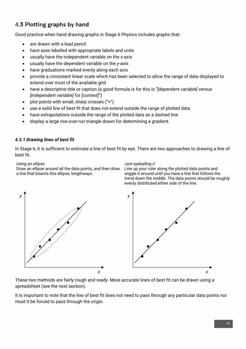
4.3 Plotting graphs by hand

Good practice when hand drawing graphs in Stage 6 Physics includes graphs that:

• are drawn with a lead pencil • have axes labelled with appropriate labels and units • usually have the independent variable on the x-axis • usually have the dependent variable on the y-axis • have graduations marked evenly along each axis • provide a consistent linear scale which has been selected to allow the range of data displayed to

extend over most of the available grid • have a descriptive title or caption (a good formula is for this is “[dependent variable] versus

[independent variable] for [context]”) • plot points with small, sharp crosses (“×”) • use a solid line of best fit that does not extend outside the range of plotted data • have extrapolations outside the range of the plotted data as a dashed line • display a large rise-over-run triangle drawn for determining a gradient.

4.3.1 Drawing lines of best fit

In Stage 6, it is sufficient to estimate a line of best fit by eye. There are two approaches to drawing a line of best fit.

Using an ellipse Draw an ellipse around all the data points, and then draw a line that bisects this ellipse, lengthways.

Just eyeballing it Line up your ruler along the plotted data points and wiggle it around until you have a line that follows the trend down the middle. The data points should be roughly evenly distributed either side of the line.

These two methods are fairly rough and ready. More accurate lines of best fit can be drawn using a spreadsheet (see the next section).

It is important to note that the line of best fit does not need to pass through any particular data points nor must it be forced to pass through the origin.

y

x

y

x

20

An example of a hand drawn graph.

Pendulum length, l (m)

Per

iod-

squa

red

T2 (s2

)

0.0 0.2 0.4 0.6 0.8 1.0

1.0

2.0

3.0

4.0

0.0

Period-squared vs length for a pendulum

Run = 0.60 m

Rise = 2.85 s2

Gradient = rise/run = 2.85/0.60 = 4.75 s2 m–1

21

5 – Using spreadsheets Spreadsheets are a powerful tool to process and analyse large amounts of data. You can try the following example, which uses Google Sheets (Microsoft Excel does the same thing in very similar ways).

5.1 Entering data

Click on a cell to select it and begin typing. Start by entering some column headings, remembering to include units. Enter your data next.

You can use the button in the tool bar to put borders around your cells and lines in your table.

5.2 Performing calculations

Next, you can perform calculations. In this example, we want to find the average of the three trials. It is important to note that spreadsheets locate data by the grid reference of the cell where it is contained.

At the top of a new column, put a heading (in this example, “Average”). In the same row as the first set of trials, type

=AVERAGE(B3,C3,D3)

And then press Enter.

The equals sign (“=”) at the start of a formula tells the spreadsheet that the cell contains a calculation, and in this example, B3, C3 and D3 are the cells that we want to average. Hitting Enter after you type a formula in a cell commands the spreadsheet to execute your calculation.

22

Equivalently, we could have typed

=AVERAGE(B3:D3)

Using a colon as in “B3:D3” indicates a contiguous range of cells – could be useful if the number of cells you are calling on is large.

We do not want to keep typing a formula into the spreadsheet over and over again if we do not have to. Instead, we can just fill down a column with copies of the formula for its respective row.

Notice that there is a small square in the bottom right corner of a selected cell. When you hover your mouse pointer over this square, it turns into a crosshair. Click and drag this crosshair down to cover the rest of the empty cells in the Average column. When you release the mouse button, the formula fills into each cell and the averages for each row should automatically be computed.

Your Average column may look like shown above, right. To reduce the number of decimal places, click on the button in the toolbar while the cells are selected until there is an appropriate number of decimal places.

Now, in this example, we want to run calculations to find the time for one period and also period squared. To do this, we will need to type some formulae into cells F3 and G3:

• We want to compute a value for one period in cell F3. Since cell E3 contains the time for ten periods we will divide this by 10. Type into cell F3:

=E3/10

• We want to compute a value for period-squared in cell G3. Since cell F3 now contains the time for one period, type into cell G3:

=F3^2

Remember to fill the formulae down the columns as before. If there are too many decimal places, use the button again while the appropriate cells are selected.

Click, drag then release

23

The completed table should look like the one below.

5.3 Plotting a graph

Select the cells in the columns of your table that you wish to use for your graph. Click in the centre of the first cell (including the column header) and drag down until the cells are selected, and then release the mouse button.

In this example, the columns are not adjacent so they cannot be selected in one step. To select column cells that are not adjacent, you will need to click and drag to select the first column (as above), release, then while holding down the Ctrl key, click, drag and release when selecting the cells of the other column.

With the cells selected, click on the button in the toolbar, or alternatively, select Insert > Chart from the menu. A graph should pop up on the screen and a Chart editor pane will open on the right.

24

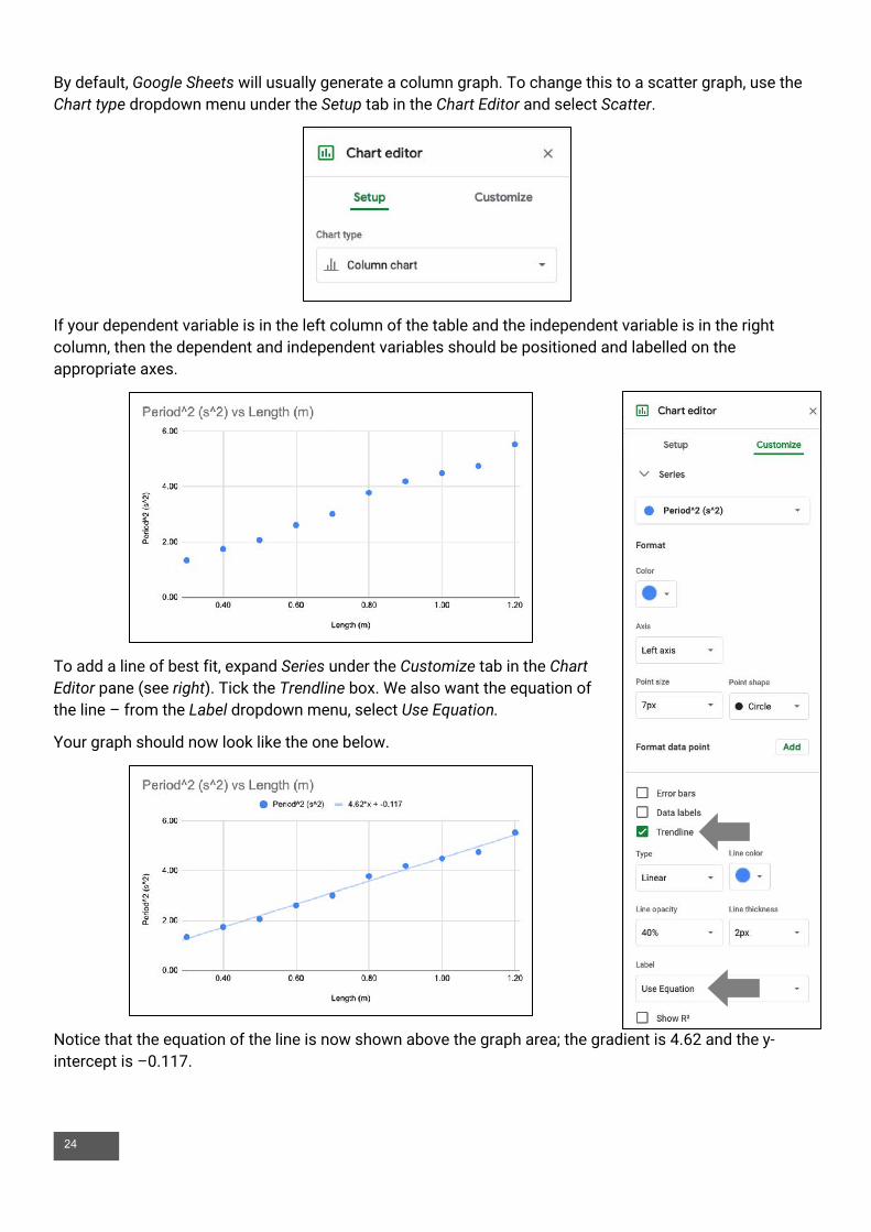
By default, Google Sheets will usually generate a column graph. To change this to a scatter graph, use the Chart type dropdown menu under the Setup tab in the Chart Editor and select Scatter.

If your dependent variable is in the left column of the table and the independent variable is in the right column, then the dependent and independent variables should be positioned and labelled on the appropriate axes.

To add a line of best fit, expand Series under the Customize tab in the Chart Editor pane (see right). Tick the Trendline box. We also want the equation of the line – from the Label dropdown menu, select Use Equation.

Your graph should now look like the one below.

Notice that the equation of the line is now shown above the graph area; the gradient is 4.62 and the y-intercept is –0.117.

25

5.4 Obtaining the uncertainty in the slope

Remember that in section 2.2.4 Uncertainty in the slope of a line of best fit, we saw that there is inherent uncertainty in the calculated gradient of a line of best fit.

There is a function in Google Sheets (“=LINEST(Y_VALUES, X_VALUES, TRUE, TRUE)”) that easily allows you to compute the uncertainty in the line (the function is the same in Microsoft Excel, but it’s a bit trickier to get Excel to display the result). It should be noted that this method does not take the uncertainty in each data point into consideration – it is looking at the spread of datapoints from the trend line.

Using our example, choose a cell below or to the right of your data (make sure this cell is clear for 5 rows down and another column right – it will fill these cells with data). Into this cell, type:

=LINEST(G3:G12, A3:A12, TRUE, TRUE)

where G3:G12 is the range of y-values and A3:A12 is the range of x-values.

When you press Enter, the function will output this array of data:

The ones we are interested in are the gradient, y-intercept, and uncertainty in the slope. The gradient can be quoted as 4.6 ± 0.2.

Notice that the gradient and y-intercept here are given to far more significant figures than that labelled on the graph.

Gradient

Uncertainty in gradient

y-intercept

Uncertainty in y-intercept

26

5.5 Common spreadsheet symbols and functions

5.5.1 Calling on cells in functions

Data in a cell can be called upon in a formula by their grid coordinate, for example, A1, B4, H27, and so on.

If a contiguous range of adjacent cells in a row, column, or block is being called upon, then a colon “:” can be used. For example:

• B4:B9 would call upon six cells in column B of the spreadsheet. • G2:K2 would call upon five cells in row 2. • B2:D5 would call on twelve cells in a rectangle between columns B to D and rows 2 to 5.

This is particularly useful when computing the average of a large number of cells, for example, =AVERAGE(D2:D99).

5.5.2 Orders of operations

Use brackets to specify order of operations. It is better to be over cautious and use more brackets than fewer if you are unsure about the order in which the spreadsheet will compute a formula. For example:

An equation that looks like this 𝑎 =𝑣 − 𝑢𝑡

would need to be entered with brackets like this =(B-A)/C

5.5.3 Entering data

Below are some special inputs for a spreadsheet.

Case Spreadsheet Example (natural) Example syntax

Pi, 𝜋 pi() 2𝜋𝑟 2*pi()*A1

Euler’s number exp(A) 𝑒! exp(2)

Scientific notation E 5.23 × 10$ 5.23E+3

27

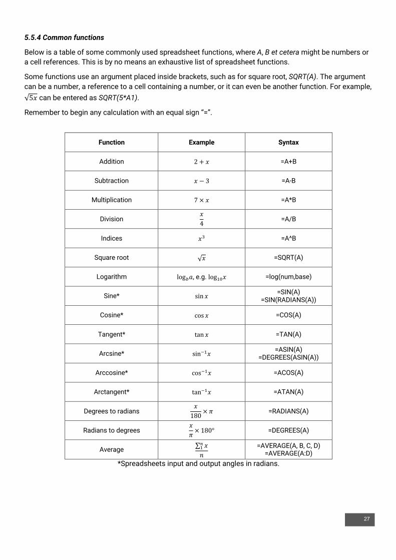
5.5.4 Common functions

Below is a table of some commonly used spreadsheet functions, where A, B et cetera might be numbers or a cell references. This is by no means an exhaustive list of spreadsheet functions.

Some functions use an argument placed inside brackets, such as for square root, SQRT(A). The argument can be a number, a reference to a cell containing a number, or it can even be another function. For example, √5𝑥 can be entered as SQRT(5*A1).

Remember to begin any calculation with an equal sign “=”.

Function Example Syntax

Addition 2 + 𝑥 =A+B

Subtraction 𝑥 − 3 =A-B

Multiplication 7 × 𝑥 =A*B

Division 𝑥4 =A/B

Indices 𝑥$ =A^B

Square root √𝑥 =SQRT(A)

Logarithm log%𝑎, e.g. log#"𝑥 =log(num,base)

Sine* sin 𝑥 =SIN(A) =SIN(RADIANS(A))

Cosine* cos 𝑥 =COS(A)

Tangent* tan 𝑥 =TAN(A)

Arcsine* sin&#𝑥 =ASIN(A) =DEGREES(ASIN(A))

Arccosine* cos&#𝑥 =ACOS(A)

Arctangent* tan&#𝑥 =ATAN(A)

Degrees to radians 𝑥180 × 𝜋 =RADIANS(A)

Radians to degrees 𝑥𝜋 × 180° =DEGREES(A)

Average ∑ 𝑥'#𝑛

=AVERAGE(A, B, C, D) =AVERAGE(A:D)

*Spreadsheets input and output angles in radians.

28

Exercises 1 Recording data 1. Write the following numbers in scientific notation.

4860 J 0.00761 m 84 kg

2. Write the following numbers in natural notation.

5.39 × 103 A 7.22 × 10–6 W 9.3 × 100 Pa

3. What orders of magnitude are these numbers?

4.734 × 107 V 6.54 × 10–5 kg 3.6155 × 103 W

4. How many significant figures are in these numbers?

15400 N 0.0007054 s 248.140 K

5. Round these numbers to three significant figures.

256 190 W 4.389 L 16.347 Ω

6. Write these observations in their base SI unit.

378 µm 0.0391 MJ 6.71 × 106 V

7. Write these observations in more convenient units.

6 428 000 V 0.0000088 W 101 800 Pa

8. Write the results of these calculations with the correct units and significant figures.

Impulse = 16.350N × 9.87s Springconstant, 𝑘 =6.89N0.025m Refractiveindex =

3.0 × 10(ms&#

2.54 × 10(ms&#

29

Exercises 2 Uncertainties 1. The accepted value for the specific heat capacity of water is accepted to be 4186 J kg–1 K–1. In an investigation

to measure it experimentally, a student produces a value of 4390 J kg–1 K–1. What is:

(a) The absolute error? (b) The relative error (as a percentage)? (c) The accuracy?

2. Calculate the relative uncertainties for the following values:

57.9 ± 0.3 m 1.7 ± 0.2 kg 2510 ± 20 years

3. Look at the following measuring devices. What uncertainty can be expected from observations using each?

4. Consider the following repeated measurements of temperature:

19.6°C, 19.4°C, 19.2°C, 19.5°C, 19.8°C Calculate the average and its uncertainty.

30

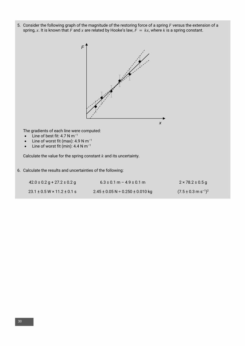
5. Consider the following graph of the magnitude of the restoring force of a spring 𝐹 versus the extension of a spring, 𝑥. It is known that 𝐹 and 𝑥 are related by Hooke’s law, 𝐹 = 𝑘𝑥, where 𝑘 is a spring constant.

The gradients of each line were computed:

• Line of best fit: 4.7 N m–1 • Line of worst fit (max): 4.9 N m–1 • Line of worst fit (min): 4.4 N m–1

Calculate the value for the spring constant 𝑘 and its uncertainty. 6. Calculate the results and uncertainties of the following:

42.0 ± 0.2 g + 27.2 ± 0.2 g 6.3 ± 0.1 m – 4.9 ± 0.1 m 2 × 78.2 ± 0.5 g

23.1 ± 0.5 W × 11.2 ± 0.1 s 2.45 ± 0.05 N ÷ 0.250 ± 0.010 kg (7.5 ± 0.3 m s–1)2

F

x

31

Exercises 3 Analysing data 1. Rewrite the following equations into the linear form 𝑌 = 𝐴𝑋 + 𝐵 given the dependent and independent

variables, and the identify the terms of the gradient.

a) For the heat required to boil varying masses of water 𝑄 = 𝑚𝑐∆𝑇

Independent variable – mass of water 𝑚 Dependent velocity – heat, 𝑄 Controlled variables – specific heat 𝑐 and change in temperature ∆𝑇 (room temp to boiling)

b) For an object undergoing uniform circular motion

𝐹 =𝑚𝑣!

𝑟 Independent variable – radius 𝑟 Dependent velocity – Centripetal force, 𝐹 Controlled variables – mass 𝑚 and linear speed 𝑣

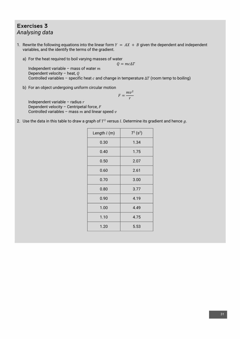
2. Use the data in this table to draw a graph of 𝑇! versus 𝑙. Determine its gradient and hence 𝑔.

Length 𝑙 (m) T2 (s2)

0.30 1.34

0.40 1.75

0.50 2.07

0.60 2.61

0.70 3.00

0.80 3.77

0.90 4.19

1.00 4.49

1.10 4.75

1.20 5.53

32

Solutions to Exercises Recording data 1. 4.86 × 103 J, 7.61 × 10–3 m, 8.4 × 101 kg 2. 5390 A, 0.00000722 W, 9.3 Pa 3. 7, –4 (because 6.54 × 10–5 rounds up to 1 × 10–4), 3 4. Three significant figures, four significant figures, six significant figures 5. 256 000 W, 4.39 L, 16.3 Ω 6. 3.78 × 10–6 m, 3.91 × 104 J, 6 710 000 V 7. 6.428 MV, 8.8 μW, 1018 hPa (meteorologists often quote atmospheric pressures in hectopascals! Otherwise 101.8 kPa is acceptable.) 8. 161 Ns, 280 Nm–1, 1.2 (no units!) Uncertainties 1. (a) 204 J kg–1 K–1 (b) 4.9% (c) 95.1% 2. 0.5%, 12%, 0.8% 3. Ruler ±0.05 cm, stopwatch ±0.005 s, protractor ±0.5°, balance ±0.05 g, digital multimeter in 10ADC mode ±0.005 A 4. 19.5 ± 0.3 °C 5. 4.7 ± 0.3 N m–1 6. 69.2 ± 0.4 g, 1.4 ± 0.2 m, 156.4 ± 1.0 g, 259 ± 8 Ws, 9.8 ± 0.6 N kg–1, 56 ± 5 m2s–2 Analysing data 1. (a) Q = cΔT·m, gradient = cΔT (b) F = mv2·1/r, gradient = mv2 (F would be graphed against 1/r) 2. See example on page 15.

References NSW Department of Education 2017, Guidelines for some working scientifically skills, accessed 3 February 2020, <https://schoolsequella.det.nsw.edu.au/file/bde20be7-b530-44ee-b8da-ba794fa4fca6/1/working-scientifically-skills-guidelines.docx> NSW Educational Standards Authority 2017, Physics stage 6 syllabus, NSW Education Standards Authority, Sydney. NSW Educational Standards Authority 2019, Physics Data Sheet, Formulae Sheet and Periodic Table for HSC exams from 2019, accessed 3 February 2020, <https://syllabus.nesa.nsw.edu.au/assets/global/files/physics-formulae-sheet-data-sheet-periodic-table-hsc-exams-2019.pdf> First Year Physics Unit 2020, First year laboratory manual, Physics 1A, School of Physics, UNSW Sydney.

33