data structures and analysis - university of torontodavid/notes/csc263.pdf · data structures and...
TRANSCRIPT

David Liu
Data Structures and AnalysisLecture Notes for CSC263 (Version 0.1)
Department of Computer ScienceUniversity of Toronto


data structures and analysis 3
These notes are based heavily on past offerings of CSC263,
and in particular the materials of François Pitt and Larry
Zhang.


Contents
1 Introduction and analysing running time 7
How do we measure running time? 7
Three different symbols 8
Worst-case analysis 9
Average-case analysis 11
Quicksort is fast on average 15
2 Priority Queues and Heaps 21
Abstract data type vs. data structure 21
The Priority Queue ADT 22
Heaps 24
Heapsort and building heaps 29
3 Dictionaries, Round One: AVL Trees 33
Naïve Binary Search Trees 34
AVL Trees 36
Rotations 38
AVL tree implementation 42
Analysis of AVL Algorithms 43

6 david liu
4 Dictionaries, Round Two: Hash Tables 47
Hash functions 47
Closed addressing (“chaining”) 48
Open addressing 52
5 Randomized Algorithms 57
Randomized quicksort 58
Universal Hashing 60
6 Graphs 63
Fundamental graph definitions 63
Implementing graphs 65
Graph traversals: breadth-first search 67
Graph traversals: depth-first search 72
Applications of graph traversals 74
Weighted graphs 79
Minimum spanning trees 80
7 Amortized Analysis 87
Dynamic arrays 87
Amortized analysis 89
8 Disjoint Sets 95
Initial attempts 95
Heuristics for tree-based disjoint sets 98
Combining the heuristics: a tale of incremental analyses 105

1 Introduction and analysing running time
Before we begin our study of different data structures and their applica-tions, we need to discuss how we will approach this study. In general, wewill follow a standard approach:
1. Motivate a new abstract data type or data structure with some examplesand reflection of previous knowledge.
2. Introduce a data structure, discussing both its mechanisms for how itstores data and how it implements operations on this data.
3. Justify why the operations are correct.
4. Analyse the running time performance of these operations.
Given that we all have experience with primitive data structures suchas arrays (or Python lists), one might wonder why we need to study datastructures at all: can’t we just do everything with arrays and pointers,already available in many languages?
Indeed, it is true that any data we want to store and any operation wewant to perform can be done in a programming language using primi-tive constructs such as these. The reason we study data structures at all,spending time inventing and refining more complex ones, is largely be-cause of the performance improvements we can hope to gain over theirmore primitive counterparts. Given the importance of this performance
This is not to say arrays and pointersplay no role. To the contrary, the studyof data structures can be viewed asthe study of how to organize andsynthesize basic programming languagecomponents in new and sophisticatedways.
analysis, it is worth reviewing what you already know about how to anal-yse the running time of algorithms, and pointing out some subtleties andcommon misconceptions you may have missed along the way.
How do we measure running time?
As we all know, the amount of time a program or single operation takesto run depends on a host of external factors – computing hardware, otherrunning processes – which the programmer has no control over.
So in our analysis we focus on just one central measure of performance:the relationship between an algorithm’s input size and the number of basic

8 david liu
operations the algorithm performs. But because even what is meant by“basic operation” can differ from machine to machine or programminglanguage to programming language, we do not try to precisely quantifythe exact number of such operations, but instead categorize how the numbergrows relative to the size of the algorithm’s input.
This is our motivation for Big-Oh notation, which is used to bring tothe foreground the type of long-term growth of a function, hiding all thenumeric constants and smaller terms that do not affect this growth. Forexample, the functions n + 1, 3n− 10, and 0.001n + log n all have the samegrowth behaviour as n gets large: they all grow roughly linearly withn. Even though these “lines” all have different slopes, we ignore theseconstants and simply say that these functions are O(n), “Big-Oh of n.” We will not give the formal definition
of Big-Oh here. For that, please consultthe CSC165 course notes.We call this type of analysis asymptotic analysis, since it deals with the
long-term behaviour of a function. It is important to remember two im-portant facts about asymptotic analysis:
• The target of the analysis is always a relationship between the size of theinput and number of basic operations performed.
What we mean by “size of the input” depends on the context, and we’llalways be very careful when defining input size throughout this course.What we mean by “basic operation” is anything whose running timedoes not depend on the size of the algorithm’s input. This is deliberately a very liberal
definition of “basic operation.” Wedon’t want you to get hung up on stepcounting, because that’s completelyhidden by Big-Oh expressions.
• The result of the analysis is a qualitative rate of growth, not an exactnumber or even an exact function. We will not say “by our asymptoticanalysis, we find that this algorithm runs in 5 steps” or even “...in 10n+
3 steps.” Rather, expect to read (and write) statements like “we find thatthis algorithm runs in O(n) time.”
Three different symbols
In practice, programmers (and even theoreticians) tend to use the Big-Ohsymbol O liberally, even when that is not exactly our meaning. However,in this course it will be important to be precise, and we will actually usethree symbols to convey different pieces of information, so you will beexpected to know which one means what. Here is a recap:
• Big-Oh. f = O(g) means that the function f (x) grows slower or at thesame rate as g(x). So we can write x2 + x = O(x2), but it is also correct Or, “g is an upper bound on the rate of
growth of f .”to write x2 + x = O(x100) or even x2 + x = O(2x).
• Omega. f = Ω(g) means that the function f (x) grows faster or at thesame rate as g(x). So we can write x2 + x = Ω(x2), but it also correct to Or, “g is a lower bound on the rate of
growth of f .”write x2 + x = Ω(x) or even x2 + x = Ω(log log x).

data structures and analysis 9
• Theta. f = Θ(g) means that the function f (x) grows at the same rateas g(x). So we can write x2 + x = Θ(x2), but not x2 + x = Θ(2x) or Or, “g has the same rate of growth as
f .”x2 + x = Θ(x).
Note: saying f = Θ(g) is equivalent to saying that f = O(g) andf = Ω(g), i.e., Theta is really an AND of Big-Oh and Omega.
Through unfortunate systemic abuse of notation, most of the time whena computer scientist says an algorithm runs in “Big-Oh of f time,” shereally means “Theta of f time.” In other words, that the function f isnot just an upper bound on the rate of growth of the running time of thealgorithm, but is in fact the rate of growth. The reason we get away withdoing so is that in practice, the “obvious” upper bound is in fact the rateof growth, and so it is (accidentally) correct to mean Theta even if one hasonly thought about Big-Oh.
However, the devil is in the details: it is not the case in this course thatthe “obvious” upper bound will always be the actual rate of growth, andso we will say Big-Oh when we mean an upper bound, and treat Thetawith the reverence it deserves. Let us think a bit more carefully about whywe need this distinction.
Worst-case analysis
The procedure of asymptotic analysis seems simple enough: look at apiece of code; count the number of basic operations performed in terms of remember, a basic operation is anything
whose runtime doesn’t depend on theinput size
the input size, taking into account loops, helper functions, and recursivecalls; then convert that expression into the appropriate Theta form.
Given any exact mathematical function, it is always possible to deter-mine its qualitative rate of growth, i.e., its corresponding Theta expression.For example, the function f (x) = 300x5 − 4x3 + x + 10 is Θ(x5), and thatis not hard to figure out.
So then why do we need Big-Oh and Omega at all? Why can’t we alwaysjust go directly from the f (x) expression to the Theta?
It’s because we cannot always take a piece of code an come up with anexact expression for the number of basic operations performed. Even ifwe take the input size as a variable (e.g., n) and use it in our counting, wecannot always determine which basic operations will be performed. Thisis because input size alone is not the only determinant of an algorithm’srunning time: often the value of the input matters as well.
Consider, for example, a function that takes a list and returns whetherthis list contains the number 263. If this function loops through the liststarting at the front, and stops immediately if it finds an occurrence of263, then in fact the running time of this function depends not just on

10 david liu
how long the list is, but whether and where it has any 263 entries.
Asymptotic notation alone cannot help solve this problem: they help usclarify how we are counting, but we have here a problem of what exactlywe are counting.
This problem is why asymptotic analysis is typically specialized toworst-case analysis. Whereas asymptotic analysis studies the relationshipbetween input size and running time, worst-case analysis studies only therelationship between input size of maximum possible running time. In otherwords, rather than answering the question “what is the running time ofthis algorithm for an input size n?” we instead aim to answer the question“what is the maximum possible running time of this algorithm for an inputsize n?” The first question’s answer might be a whole range of values; thesecond question’s answer can only be a single number, and that’s how weget a function involving n.
Some notation: we typically use the name T(n) to represent the maxi-mum possible running time as a function of n, the input size. The resultof our analysis, could be something like T(n) = Θ(n), meaning that theworst-case running time of our algorithm grows linearly with the inputsize.
Bounding the worst case
But we still haven’t answered the question: where do O and Ω come in?The answer is basically the same as before: even with this more restrictednotion of worst-case running time, it is not always possible to calculate anexact expression for this function. What is usually easy to do, however, iscalculate an upper bound on the maximum number of operations. One suchexample is the likely familiar line of reasoning, “the loop will run at mostn times” when searching for 263 in a list of length n. Such analysis, whichgives a pessimistic outlook on the most number of operations that couldtheoretically happen, results in an exact count – e.g., n + 1 – which is anupper bound on the maximum number of operations. From this analysis,we can conclude that T(n), the worst-case running time, is O(n).
What we can’t conclude is that T(n) = Ω(n). There is a subtle impli-cation of the English phrase “at most.” When we say “you can have atmost 10 chocolates,” it is generally understood that you can indeed haveexactly 10 chocolates; whatever number is associated with “at most” isachievable.
In our analysis, however, we have no way of knowing that the upperbound we obtain by being pessimistic in our operation counting is ac-tually achievable. This is made more obvious if we explicitly mentionthe fact that we’re studying the maximum possible number of operations:

data structures and analysis 11
“the maximum running time is less than or equal to n + 1” surely sayssomething different than “the maximum running time is equal to n + 1.”
So how do we show that whatever upper bound we get on the max-imum is actually achievable? In practice, we rarely try to show that theexact upper bound is achievable, since that doesn’t actually matter. In-stead, we try to show that an asymptotic lower bound – a Omega – isachievable. For example, we want to show that the maximum runningtime is Ω(n), i.e., grows at least as quickly as n.
To show that the maximum running time grows at least as quickly assome function f , we need to find a family of inputs, one for each inputsize n, whose running time has a lower bound of f (n). For example, forour problem of searching for 263 in a list, we could say that the family ofinputs is “lists that contain only 0’s.” Running the search algorithm onsuch a list of length n certainly requires checking each element, and so thealgorithm takes at least n basic operations. From this we can conclude thatthe maximum possible running time is Ω(n). Remember, the constants don’t matter.
The family of inputs which contain only1’s for the first half, and only 263’s forthe second half, would also have givenus the desired lower bound.
To summarize: to perform a complete worst-case analysis and get atight, Theta bound on the worst-case running time, we need to do thefollowing two things:
(i) Give a pessimistic upper bound on the number of basic operations thatcould occur for any input of a fixed size n. Obtain the correspondingBig-Oh expression (i.e., T(n) = O( f )). Observe that (i) is proving something
about all possible inputs, while (ii) isproving something about just one familyof inputs.
(ii) Give a family of inputs (one for each input size), and give a lower bound onthe number of basic operations that occurs for this particular family ofinputs. Obtain the corresponding Omega expression (i.e., T(n) = Ω( f )).
If you have performed a careful enough analysis in (i) and chosen agood enough family in (ii), then you’ll find that the Big-Oh and Omegaexpressions involve the same function f , and which point you can con-clude that the worst-case running time is T(n) = Θ( f ).
Average-case analysis
So far in your career as computer scientists, you have been primarily con-cerned with the worst-case algorithm analysis. However, in practice thistype of analysis often ends up being misleading, with a variety of al-gorithms and data structures having a poor worst-case performance stillperforming well on the majority of possible inputs.
Some reflection makes this not too surprising; focusing on the maxi-mum of a set of numbers (like running times) says very little about the“typical” number in that set, or, more precisely, the distribution of num-

12 david liu
bers within that set. In this section, we will learn a powerful new tech-nique that enables us to analyse some notion of “typical” running time foran algorithm.
Warmup
Consider the following algorithm, which operates on a non-empty arrayof integers:
1 def evens_are_bad(lst):
2 if every number in lst is even:
3 repeat lst.length times:
4 calculate and print the sum of lst
5 return 1
6 else:
7 return 0
Let n represent the length of the input list lst. Suppose that lst con-tains only even numbers. Then the initial check on line 2 takes Ω(n) time,while the computation in the if branch takes Ω(n2) time. This means that We leave it as an exercise to justify why
the if branch takes Ω(n2) time.the worst-case running time of this algorithm is Ω(n2). It is not too hardto prove the matching upper bound, and so the worst-case running timeis Θ(n2).
However, the loop only executes when every number in lst is even;when just one number is odd, the running time is O(n), the maximumpossible running time of executing the all-even check. Intuitively, it seems Because executing the check might
abort quickly if it finds an odd numberearly in the list, we used the pessimisticupper bound of O(n) rather than Θ(n).
much more likely that not every number in lst is even, so we expect themore “typical case” for this algorithm is to have a running time boundedabove as O(n), and only very rarely to have a running time of Θ(n2).
Our goal now is to define precisely what we mean by the “typical case”for an algorithm’s running time when considering a set of inputs. Asis often the case when dealing with the distribution of a quantity (likerunning time) over a set of possible values, we will use our tools fromprobability theory to help achieve this.
We define the average-case running time of an algorithm to be thefunction Tavg(n) which takes a number n and returns the (weighted) aver-age of the algorithm’s running time for all inputs of size n.
For now, let’s ignore the “weighted” part, and just think of Tavg(n) ascomputing the average of a set of numbers. What can we say about theaverage-case for the function evens_are_bad? First, we fix some input sizen. We want to compute the average of all running times over all input listsof length n.

data structures and analysis 13
At this point you might be thinking, “well, each number is even withprobability one-half, so...” This is a nice thought, but a little premature –the first step when doing an average-case analysis is to define the possibleset of inputs. For this example, we’ll start with a particularly simple setof inputs: the lists whose elements are between 1 and 5, inclusive.
The reason for choosing such a restricted set is to simplify the calcu-lations we need to perform when computing an average. Furthermore,because the calculation requires precise numbers to work with, we willneed to be precise about what “basic operations” we’re counting. For thisexample, we’ll count only the number of times a list element is accessed,either to check whether it is even, or when computing the sum of the list.So a “step” will be synonymous with “list access.”
It is actually fairly realistic to focussolely on operations of a particulartype in a runtime analysis. We typicallychoose the operation that happens themost frequently (as in this case), orthe one which is the most expensive.Of course, the latter requires that weare intimately knowledgeable aboutthe low-level details of our computingenvironment.
The preceding paragraph is the work of setting up the context of ouranalysis: what inputs we’re looking at, and how we’re measuring runtime.The final step is what we had initially talked about: compute the averagerunning time over inputs of length n. This often requires some calcu-lation, so let’s get to it. To simplify our calculations even further, we’llassume that the all-evens check on line 2 always accesses all n elements. You’ll explore the “return early” variant
in an exercise.In the loop, there are n2 steps (each number is accessed n times, once pertime the sum is computed).
There are really only two possibilities: the lists that have all even num-bers will run in n2 + n steps, while all the other lists will run in just nsteps. How many of each type of list are there? For each position, thereare two possible even numbers (2 and 4), so the number of lists of lengthn with every element being even is 2n. That sounds like a lot, but consider In the language of counting: make
n independent decisions, with eachdecision having two choices.
that there are five possible values per element, and hence 5n possible in-puts in all. So 2n inputs have all even numbers and take n2 + n steps,while the remaining 5n − 2n inputs take n steps. Number Steps
all even 2n n2 + nthe rest 5n − 2n nThe average running time is:
Tavg(n) =2n(n2 + n) + (5n − 2n)n
5n (5n inputs total)
=2nn2
5n + n
=
(25
)nn2 + n
= Θ(n)Remember that any exponential growsfaster than any polynomial, so that firstterm goes to 0 as n goes to infinity.
This analysis tells us that the average-case running time of this algo-rithm is Θ(n), as our intuition originally told us. Because we computedan exact expression for the average number of steps, we could convert thisdirectly into a Theta expression.
As is the case with worst-case analysis,it won’t always be so easy to computean exact expression for the average,and in those cases the usual upper andlower bounding must be done.

14 david liu
The probabilistic view
The analysis we performed in the previous section was done through thelens of counting the different kinds of inputs and then computing the av-erage of their running times. However, there is a more powerful tech-nique that you know about: treating the algorithm’s running time as arandom variable T, defined over the set of possible inputs of size n. Wecan then redo the above analysis in this probabilistic context, performingthese steps:
1. Define the set of possible inputs and a probability distribution over thisset. In this case, our set is all lists of length n that contain only ele-ments in the range 1-5, and the probability distribution is the uniformdistribution. Recall that the uniform distribution
assigns equal probability to eachelement in the set.2. Define how we are measuring runtime. (This is unchanged from the
previous analysis.)
3. Define the random variable T over this probability space to representthe running time of the algorithm. Recall that a random variable is a
function whose domain is the set ofinputs.In this case, we have the nice definition
T =
n2 + n, input contains only even numbers
n, otherwise
4. Compute the expected value of T, using the chosen probability dis-tribution and formula for T. Recall that the expected value of a vari-able is determined by taking the sum of the possible values of T, eachweighted by the probability of obtaining that value.
E[T] = ∑t
t · Pr[T = t]
In this case, there are only two possible values for T:
E[T] = (n2 + n) · Pr[the list contains only even numbers]
+ n · Pr[the list contains at least one odd number]
= (n2 + n) ·(
25
)n+ n ·
(1−
(25
)n)= n2 ·
(25
)n+ n
= Θ(n)
Of course, the calculation ended up being the same, even if we ap-proached it a little differently. The point to shifting to using probabilities

data structures and analysis 15
is in unlocking the ability to change the probability distribution. Rememberthat our first step, defining the set of inputs and probability distribution,is a great responsibility of the ones performing the runtime analysis. Howin the world can we choose a “reasonable” distribution? There is a ten- What does it mean for a distribution to
be “reasonable,” anyway?dency for us to choose distributions that are easy to analyse, but of coursethis is not necessarily a good criterion for evaluating an algorithm.
By allowing ourselves to choose not only what inputs are allowed, butalso give relative probabilities of those inputs, we can use the exact sametechnique to analyse an algorithm under several different possible scenar-ios – this is both the reason we use “weighted average” rather than simply“average” in our above definition of average-case, and also how we areable to calculate it.
Exercise Break!
1.1 Prove that the evens_are_bad algorithm on page 12 has a worst-caserunning time of O(n2), where n is the length of the input list.
1.2 Consider this alternate input space for evens_are_bad: each element in
the list is even with probability99100
, independent of all other elements.Prove that under this distribution, the average-case running time is stillΘ(n).
1.3 Suppose we allow the “all-evens” check in evens_are_bad to stop im-mediately after it finds an odd element. Perform a new average-caseanalysis for this mildly-optimized version of the algorithm using thesame input distribution as in the notes.
Hint: the running time T now can take on any value between 1 and n;first compute the probability of getting each of these values, and thenuse the expected value formula.
Quicksort is fast on average
The previous example may have been a little underwhelming, since it was“obvious” that the worst-case was quite rare, and so not surprising thatthe average-case running time is asymptotically faster than the worst-case.However, this is not a fact you should take for granted. Indeed, it is oftenthe case that algorithms are asymptotically no better “on average” thanthey are in the worst-case. Sometimes, though, an algorithm can have a Keep in mind that because asymptotic
notation hides the constants, saying twofunctions are different asymptotically ismuch more significant than saying thatone function is “bigger” than another.
significantly better average case than worst case, but it is not nearly asobvious; we’ll finish off this chapter by studying one particularly well-known example.

16 david liu
Recall the quicksort algorithm, which takes a list and sorts it by choos-ing one element to be the pivot (say, the first element), partitioning theremaining elements into two parts, those less than the pivot, and thosegreater than the pivot, recursively sorting each part, and then combiningthe results.
1 def quicksort(array):
2 if array.length < 2:
3 return
4 else:
5 pivot = array[0]
6 smaller, bigger = partition(array[1:], pivot)
7 quicksort(smaller)
8 quicksort(bigger)
9 array = smaller + [pivot] + bigger # array concatenation
10
11 def partition(array, pivot):
12 smaller = []
13 bigger = []
14 for item in array:
15 if item <= pivot:
16 smaller.append(item)
17 else:
18 bigger.append(item)
19 return smaller, bigger
This version of quicksort uses linear-size auxiliary storage; we chose thisbecause it is a little simpler to writeand analyse. The more standard “in-place” version of quicksort has thesame running time behaviour, it justuses less space.
You have seen in previous courses that the choice of pivot is crucial, asit determines the size of each of the two partitions. In the best case, thepivot is the median, and the remaining elements are split into partitions ofroughly equal size, leading to a running time of Θ(n log n), where n is thesize of the list. However, if the pivot is always chosen to be the maximumelement, then the algorithm must recurse on a partition that is only oneelement smaller than the original, leading to a running time of Θ(n2).
So given that there is a difference between the best- and worst-caserunning times of quicksort, the next natural question to ask is: What isthe average-case running time? This is what we’ll answer in this section.
First, let n be the length of the list. Our set of inputs is all possiblepermutations of the numbers 1 to n (inclusive). We’ll assume any of these Our analysis will therefore assume the
lists have no duplicates.n! permutations are equally likely; in other words, we’ll use the uniformdistribution over all possible permutations of 1, . . . , n. We will measureruntime by counting the number of comparisons between elements in the listin the partition function.

data structures and analysis 17
Let T be the random variable counting the number of comparisonsmade. Before starting the computation of E[T], we define additional ran-dom variables: for each i, j ∈ 1, . . . , n with i < j, let Xij be the indicatorrandom variable defined as:
Xij =
1, if i and j are compared
0, otherwise
Because each pair is compared at most once, we obtain the total number
Remember, this is all in the context ofchoosing a random permutation.
of comparisons simply by adding these up:
T =n
∑i=1
n
∑j=i+1
Xij.
The purpose of decomposing T into a sum of simpler random variablesis that we can now apply the linearity of expectation (see margin note). If X, Y, and Z are random variables and
X = Y + Z, then E[X] = E[Y] + E[Z],even if Y and Z are dependent.
E[T] =n
∑i=1
n
∑j=i+1
E[Xij]
=n
∑i=1
n
∑j=i+1
Pr[i and j are compared] Recall that for an indicator variable, itsexpected value is simply the probabilitythat it takes on the value 1.
To make use of this “simpler” form, we need to investigate the prob-ability that i and j are compared when we run quicksort on a randomarray.
Proposition 1.1. Let 1 ≤ i < j ≤ n. The probability that i and j are comparedwhen running quicksort on a random permutation of 1, . . . , n is 2/(j− i + 1).
Proof. First, let us think about precisely when elements are compared witheach other in quicksort. Quicksort works by selecting a pivot element,then comparing the pivot to every other item to create two partitions, andthen recursing on each partition separately. So we can make the followingobservations:
(i) Every comparison must involve the “current” pivot.
(ii) The pivot is only compared to the items that have always been placedinto the same partition as it by all previous pivots. Or, once two items have been put into
different partitions, they will never becompared.
So in order for i and j to be compared, one of them must be chosen asthe pivot while the other is in the same partition. What could cause i andj to be in different partitions? This only happens if one of the numbersbetween i and j (exclusive) is chosen as a pivot before i or j is chosen.

18 david liu
So then i and j are compared by quicksort if and only if one of them isselected to be pivot first out of the set of numbers i, i + 1, . . . , j.
Because we’ve given an implementation of quicksort that always choosesthe first item to be the pivot, the item which is chosen first as pivot mustbe the one that appears first in the random input permutation. Since Of course, the input list contains other
numbers, but because our partitionalgorithm preserves relative orderwithin a partition, if a appears beforeb in the original list, then a will stillappear before b in every subsequentpartition that contains them both.
we choose the permutation uniformly at random, each item in the seti, . . . , j is equally likely to appear first, and thus be chosen first as pivot.
Finally, because there are j− i + 1 numbers in this set, the probabilitythat either i or j is chosen first is 2/(j− i + 1), and this is the probabilitythat i and j are compared.
Now that we have this probability computed, we can return to ourexpected value calculation to complete our average-case analysis.
Theorem 1.2 (Quicksort average-case runtime). The average number of com-parisons made by quicksort on a uniformly chosen random permutation of 1, . . . , nis Θ(n log n).
Proof. As before, let T be the random variable representing the runningtime of quicksort. Our previous calculations together show that
E[T] =n
∑i=1
n
∑j=i+1
Pr[i and j are compared]
=n
∑i=1
n
∑j=i+1
2j− i + 1
=n
∑i=1
n−i
∑j′=1
2j′ + 1
(change of index j′ = j− i)
= 2n
∑i=1
n−i
∑j′=1
1j′ + 1 i j′ values
1 1, 2, 3, . . . , n− 2, n− 12 1, 2, 3, . . . , n− 2...
...n− 3 1, 2, 3n− 2 1, 2n− 1 1
n
Now, note that the individual terms of the inner summation don’t de-pend on i, only the bound does. The first term, when j′ = 1, occurs when1 ≤ i ≤ n − 1, or n − 1 times in total; the second (j′ = 2) occurs wheni ≤ n− 2, and in general the j′ = k term appears n− k times.
So we can simplify the counting to eliminate the summation over i:

data structures and analysis 19
E[T] = 2n−1
∑j′=1
n− j′
j′ + 1
= 2n−1
∑j′=1
(n + 1j′ + 1
− 1)
= 2(n + 1)n−1
∑j′=1
1j′ + 1
− 2(n− 1)
We will use the fact from mathematics that the functionn
∑i=1
1i + 1
is
Θ(log n), and so we get that E[T] = Θ(n log n). Actually, we know something stronger:we even know that the constant hiddenin the Θ is equal to 1.
Exercise Break!
1.4 Review the insertion sort algorithm, which builds up a sorted list byrepeatedly inserting new elements into a sorted sublist (usually at thefront). We know that its worst-case running time is Θ(n2), but its bestcase is Θ(n), even better than quicksort. So does it beat quicksort onaverage?
Suppose we run insertion sort on a random permutation of the numbers1, . . . , n, and consider counting the number of swaps as the runningtime. Let T be the random variable representing the total number ofswaps.
(a) For each 1 ≤ i ≤ n, define the random variable Si to be the numberof swaps made when i is inserted into the sorted sublist.
Express T in terms of Si.
(b) For each 1 ≤ i, j ≤ n, define the random indicator variables Xij that is1 if i and j are swapped during insertion sort.
Express Si in terms of the Xij.
(c) Prove that E[Xij] = 1/2.
(d) Show that the average-case running time of insertion sort is Θ(n2).


2 Priority Queues and Heaps
In this chapter, we will study our first major data structure: the heap. Asthis is our first extended analysis of a new data structure, it is important topay attention to the four components of this study outlined at the previouschapter:
1. Motivate a new abstract data type or data structure with some examplesand reflection of previous knowledge.
2. Introduce a data structure, discussing both its mechanisms for how itstores data and how it implements operations on this data.
3. Justify why the operations are correct.
4. Analyse the running time performance of these operations.
Abstract data type vs. data structure
The study of data structures involves two principal, connected pieces: aspecification of what data we want to store and operations we want tosupport, and an implementation of this data type. We tend to blur theline between these two components, but the difference between them isfundamental, and we often speak of one independently of the other. Sobefore we jump into our first major data structure, let us remind ourselvesof the difference between these two.
Definition 2.1 (abstract data type, data structure). An abstract data type(ADT) is a theoretical model of an entity and the set of operations thatcan be performed on that entity. The key term is abstract: an ADT is a
definition that can be understood andcommunicated without any code at all.A data structure is a value in a program which can be used to store and
operate on data.
For example, contrast the difference between the List ADT and an arraydata structure.

22 david liu
List ADT
• Length(L): Return the number of items in L.
• Get(L, i): Return the item stored at index i in L.
• Store(L, i, x): Store the item x at index i in L.
There may be other operations youthink are fundamental to lists; we’vegiven as bare-bones a definition aspossible.
This definition of the List ADT is clearly abstract: it specifies what thepossible operations are for this data type, but says nothing at all abouthow the data is stored, or how the operations are performed.
It may be tempting to think of ADTs as the definition of interfaces orabstract classes in a programming language – something that specifies acollection of methods that must be implemented – but keep in mind thatit is not necessary to represent an ADT in code. A written description ofthe ADT, such as the one we gave above, is perfectly acceptable.
On the other hand, a data structure is tied fundamentally to code. Itexists as an entity in a program; when we talk about data structures, wetalk about how we write the code to implement them. We are aware ofnot just what these data structures do, but how they do them.
When we discuss arrays, for example, we can say that they implementthe List ADT; i.e., they support the operations defined in the List ADT.However, we can say much more than this:
• Arrays store elements in consecutive locations in memory
• They perform Get and Store in constant time with respect to thelength of the array.
• How Length is supported is itself an implementation detail specificto a particular language. In C, arrays must be wrapped in a struct tomanually store their length; in Java, arrays have a special immutableattribute called length; in Python, native lists are implemented using At least, the standard CPython imple-
mentation of Python.arrays an a member to store length.
The main implementation-level detail that we’ll care about this in courseis the running time of an operation. This is not a quantity that can be spec-ified in the definition of an ADT, but is certainly something we can study ifwe know how an operation is implemented in a particular data structure.
The Priority Queue ADT
The first abstract data type we will study is the Priority Queue, which issimilar in spirit to the stacks and queues that you have previously studied.

data structures and analysis 23
Like those data types, the priority queue supports adding and removingan item from a collection. Unlike those data types, the order in whichitems are removed does not depend on the order in which they are added,but rather depends on a priority which is specified when each item isadded.
A classic example of priority queues in practice is a hospital waitingroom: more severe injuries and illnesses are generally treated before minorones, regardless of when the patients arrived at the hospital.
Priority Queue ADT
• Insert(PQ, x, priority): Add x to the priority queue PQ with the givenpriority.
• FindMax(PQ): Return the item in PQ with the highest priority.
• ExtractMax(PQ): Remove and return the item from PQ with thehighest priority.
As we have already discussed, one of the biggest themes of this courseis the distinction between the definition of an abstract data type, and theimplementation of that data type using a particular data structure. To em- One can view most hospital waiting
rooms as a physical, buggy implemen-tation of a priority queue.
phasize that these are separate, we will first give a naïve implementationof the Priority Queue ADT that is perfectly correct, but inefficient. Then,we will contrast this approach with one that uses the heap data structure.
A basic implementation
Let us consider using an unsorted linked list to implement a priorityqueue. In this case, adding a new item to the priority queue can be donein constant time: simply add the item and corresponding priority to thefront of the linked list. However, in order to find or remove the itemwith the lowest priority, we must search through the entire list, which is alinear-time operation.
Given a new ADT, it is often helpful to come up with a “naïve” or“brute force” implementation using familiar primitive data structures likearrays and linked lists. Such implementations are usually quick to comeup with, and analysing the running time of the operations is also usuallystraight-forward. Doing this analysis gives us targets to beat: given thatwe can code up an implementation of priority queue which supports In-sert in Θ(1) time and FindMax and ExtractMax in Θ(n) time, can wedo better using a more complex data structure? The rest of this chapter isdevoted to answering this question.

24 david liu
1 def Insert(PQ, x, priority):
2 n = Node(x, priority)
3 oldHead = PQ.head
4 n.next = old_head
5 PQ.head = n
6
7
8 def FindMax(PQ):
9 n = PQ.head
10 maxNode = None
11 while n is not None:
12 if maxNode is None or n.priority > maxNode.priority:
13 maxNode = n
14 n = n.next
15 return maxNode.item
16
17
18 def ExtractMax(PQ):
19 n = PQ.head
20 prev = None
21 maxNode = None
22 prevMaxNode = None
23 while n is not None:
24 if maxNode is None or n.priority > maxNode.priority:
25 maxNode, prevMaxNode = n, prevNode
26 prev, n = n, n.next
27
28 if prevMaxNode is None:
29 self.head = maxNode.next
30 else:
31 prevMaxNode.next = maxNode.next
32
33 return maxNode.item
Heaps
Recall that a binary tree is a tree in which every node has at most twochildren, which we distinguish by calling the left and right. You probablyremember studying binary search trees, a particular application of a binarytree that can support fast insertion, deletion, and search. We’ll look at a more advanced form of
binary search trees in the next chapter.Unfortunately, this particular variant of binary trees does not exactly
suit our purposes, since the item with the highest priority will generally

data structures and analysis 25
be at or near the bottom of a BST. Instead, we will focus on a variation ofbinary trees that uses the following property:
Definition 2.2 (heap property). A tree satisfies the heap property if andonly if for each node in the tree, the value of that node is greater than orequal to the value of all of its descendants.
Alternatively, for any pair of nodes a, b in the tree, if a is an ancestor ofb, then the value of a is greater than or equal to the value of b.
This property is actually less stringent than the BST property: givena node which satisfies the heap property, we cannot conclude anythingabout the relationships between its left and right subtrees. This meansthat it is actually much easier to get a compact, balanced binary tree thatsatisfies the heap property than one that satisfies the BST property. In fact,we can get away with enforcing as strong a balancing as possible for ourdata structure.
Definition 2.3 (complete binary tree). A binary tree is complete if andonly if it satisfies the following two properties:
• All of its levels are full, except possibly the bottom one. Every leaf must be in one of the twobottommost levels.
• All of the nodes in the bottom level are as far to the left as possible.A
B C
D E F
Complete trees are essentially the trees which are most “compact.” Acomplete tree with n nodes has dlog ne height, which is the smallest pos-sible height for a tree with this number of nodes.
Moreover, because we also specify that the nodes in the bottom layermust be as far left as possible, there is never any ambiguity about wherethe “empty” spots in a complete tree are. There is only one complete treeshape for each number of nodes.
Because of this, we do not need to use up space to store references be-tween nodes, as we do in a standard binary tree implementation. Instead,we fix a conventional ordering of the nodes in the heap, and then simplywrite down the items in the heap according to that order. The order weuse is called level order, because it orders the elements based on their depthin the tree: the first node is the root of the tree, then its children (at depth1) in left-to-right order, then all nodes at depth 2 in left-to-right order, etc.
The array representation of the abovecomplete binary tree.
A B C D E FWith these two definitions in mind, we can now define a heap.
Definition 2.4 (heap). A heap is a binary tree that satisfies the heap propertyand is complete.
We implement a heap in a program as an array, where the items in thearray correspond to the level order of the actual binary tree. This is a nice example of how we use
primitive data structures to buildmore complex ones. Indeed, a heap isnothing sophisticated from a technicalstandpoint; it is merely an array whosevalues are ordered in a particular way.

26 david liu
A note about array indices
In addition to being a more compact representation of a complete binarytree, this array representation has a beautiful relationship between theindices of a node in the tree and those of its children.
We assume the items are stored starting at index 1 rather than 0, whichleads to the following indices for the nodes in the tree.
1
2 3
4 5 6 7
8 9 10 11 12
We are showing the indices where eachnode would be stored in the array.
A pattern quickly emerges. For a node corresponding to index i, itsleft child is stored at index 2i, and its right child is stored at index 2i + 1.Going backwards, we can also deduce that the parent of index i (wheni > 1) is stored at index bi/2c. This relationship between indices willprove very useful in the following section when we start performing morecomplex operations on heaps.
Heap implementation of a priority queue
Now that we have defined the heap data structure, let us see how to useit to implement the three operations of a priority queue.
FindMax becomes very simple to both implement and analyse, be-cause the root of the heap is always the item with the maximum priority,and in turn is always stored at the front of the array.
Remember that indexing starts at 1
rather than 0.
1 def FindMax(PQ):
2 return PQ[1]
Remove is a little more challenging. Obviously we need to remove theroot of the tree, but how do we decide what to replace it with? One keyobservation is that because the resulting heap must still be complete, weknow how its structure must change: the very last (rightmost) leaf mustno longer appear.

data structures and analysis 27
Rightmost leaf 17 is moved to the root.
50
30 45
28 20 16 2
8 19 17
17 is swapped with 45 (since 45 isgreater than 30).
17
30 45
28 20 16 2
8 19
So our first step is to save the root of the tree, and then replace it withthe last leaf. (Note that we can access the leaf in constant time because weknow the size of the heap, and the last leaf is always at the end of the listof items.)
No more swaps occur; 17 is greaterthan both 16 and 2.
45
30 17
28 20 16 2
8 19
But the last leaf priority is smaller than many other priorities, and so ifwe leave the heap like this, the heap property will be violated. Our laststep is to repeatedly swap the moved value with one of its children untilthe heap property is satisfied once more. On each swap, we choose thelarger of the two children to ensure that the heap property is preserved.
The repeated swapping is colloquiallycalled the “bubble down” step, refer-ring to how the last leaf starts at thetop of the heap and makes its way backdown in the loop.
1 def ExtractMax(PQ):
2 temp = PQ[1]
3 PQ[1] = PQ[PQ.size] # Replace the root with the last leaf
4 PQ.size = PQ.size - 1
5
6 # Bubble down
7 i = 1
8 while i < PQ.size:
9 curr_p = PQ[i].priority
10 left_p = PQ[2*i].priority
11 right_p = PQ[2*i + 1].priority
12
13 # heap property is satisfied
14 if curr_p >= left_p and curr_p >= right_p:
15 break
16 # left child has higher priority
17 else if left_p >= right_p:
18 PQ[i], PQ[2*i] = PQ[2*i], PQ[i]
19 i = 2*i
20 # right child has higher priority
21 else:
22 PQ[i], PQ[2*i + 1] = PQ[2*i + 1], PQ[i]
23 i = 2*i + 1
24
25 return temp
What is the running time of this algorithm? All individual lines of codetake constant time, meaning the runtime is determined by the number ofloop iterations.
At each iteration, either the loop stops immediately, or i increases by atleast a factor of 2. This means that the total number of iterations is at most

28 david liu
log n, where n is the number of items in the heap. The worst-case runningtime of Remove is therefore O(log n).
The implementation of Insert is similar. We again use the fact thatthe number of items in the heap completely determines its structure: inthis case, because a new item is being added, there will be a new leafimmediately to the right of the current final leaf, and this corresponds tothe next open position in the array after the last item.
So our algorithm simply puts the new item there, and then performsan inverse of the swapping from last time, comparing the new item withits parent, and swapping if it has a larger priority. The margin diagramsshow the result of adding 35 to the given heap. A “bubble up” instead of “bubble
down”
45
30 17
28 20 16 2
8 19 35
45
30 17
28 35 16 2
8 19 20
45
35 17
28 30 16 2
8 19 20
35 is swapped twice with its parent (20,then 30), but does not get swapped with45.
1 def Insert(PQ, x, priority):
2 PQ.size = PQ.size + 1
3 PQ[PQ.size].item = x
4 PQ[PQ.size].priority = priority
5
6 i = PQ.size
7 while i > 1:
8 curr_p = PQ[i].priority
9 parent_p = PQ[i // 2].priority
10
11 if curr_p <= parent_p: # PQ property satisfied, break
12 break
13 else:
14 PQ[i], PQ[i // 2] = PQ[i // 2], PQ[i]
15 i = i // 2
Again, this loop runs at most log n iterations, where n is the numberof items in the heap. The worst-case running time of this algorithm istherefore O(log n).
Runtime summary
Let us compare the worst-case running times for the three operations forthe two different implementations we discussed in this chapter. In thistable, n refers to the number of elements in the priority queue. Operation Linked list Heap
Insert Θ(1) Θ(log n)FindMax Θ(n) Θ(1)
ExtractMax Θ(n) Θ(log n)
This table nicely illustrates the tradeoffs generally found in data struc-ture design and implementation. We can see that heaps beat unsortedlinked lists in two of the three priority queue operations, but are asymp-totically slower than unsorted linked lists when adding a new element.

data structures and analysis 29
Now, this particular case is not much of a choice: that the slowest oper-ation for heaps runs in Θ(log n) time in the worst case is substantiallybetter than the corresponding Θ(n) time for unsorted linked lists, and inpractice heaps are indeed widely used.
The reason for the speed of the heap operations is the two properties –the heap property and completeness – that are enforced by the heap datastructures. These properties impose a structure on the data that allowsus to more quickly extract the desired information. The cost of theseproperties is that they must be maintained whenever the data structure ismutated. It is not enough to take a new item and add it to the end of theheap array; it must be “bubbled up” to its correct position to maintain theheap property, and this is what causes the Insert operation to take longer.
Heapsort and building heaps
In our final section of this chapter, we will look at one interesting applica-tion of heaps to a fundamental task in computer science: sorting. Givena heap, we can extract a sorted list of the elements in the heap simply byrepeatedly calling Remove and adding the items to a list. Of course, this technically sorts by
priority of the items. In general, givena list of values to sort, we would treatthese values as priorities for the pur-pose of priority queue operations.
However, to turn this into a true sorting algorithm, we need a way ofconverting an input unsorted list into a heap. To do this, we interpretthe list as the level order of a complete binary tree, same as with heaps.The difference is that this binary tree does not necessarily satisfy the heapproperty, and it is our job to fix it.
We can do this by performing the “bubble down” operation on eachnode in the tree, starting at the bottom node and working our way up.
1 def BuildHeap(items):
2 i = items.length
3 while i > 0:
4 BubbleDown(items, i)
5 i = i - 1
6
7 def BubbleDown(heap, i):
8 while i < heap.size:
9 curr_p = heap[i].priority
10 left_p = heap[2*i].priority
11 right_p = heap[2*i + 1].priority
12
13 # heap property is satisfied
14 if curr_p >= left_p and curr_p >= right_p:
15 break

30 david liu
16 # left child has higher priority
17 else if left_p >= right_p:
18 PQ[i], PQ[2*i] = PQ[2*i], PQ[i]
19 i = 2*i
20 # right child has higher priority
21 else:
22 PQ[i], PQ[2*i + 1] = PQ[2*i + 1], PQ[i]
23 i = 2*i + 1
What is the running time of this algorithm? Let n be the length ofitems. Then the loop in BubbleDown iterates at most log n times; sinceBubbleDown is called n times, this means that the worst-case runningtime is O(n log n).
However, this is a rather loose analysis: after all, the larger i is, thefewer iterations the loop runs. And in fact, this is a perfect example of asituation where the “obvious” upper bound on the worst-case is actuallynot tight, as we shall soon see.
To be more precise, we require a better understanding of how long Bub-bleDown takes to run as a function of i, and not just the length of items.Let T(n, i) be the maximum number of loop iterations of BubbleDown
for input i and a list of length n. Then the total number of iterations in Note that T, a runtime function, hastwo inputs, reflecting our desire toincorporate both i and n in our analysis.all n calls to BubbleDown from BuildHeap is
n
∑i=1
T(n, i). So how do we
compute T(n, i)? The maximum number of iterations is simply the heighth of node i in the complete binary tree with n nodes. Each iteration goes down one level in
the tree.So we can partition the nodes based on their height:
n
∑i=1
T(i, n) =k
∑h=1
h · # nodes at height h
1
2 3
4 5 6 7
8 9 10 11 12 13 14 15
The final question is, how many nodes are at height h in the tree? Tomake the analysis simpler, suppose the tree has height k and n = 2k − 1nodes; this causes the binary tree to have a full last level. Consider thecomplete binary tree shown at the right (k = 4). There are 8 nodes atheight 1 (the leaves), 4 nodes at height 2, 2 nodes at height 3, and 1 nodeat height 4 (the root). In general, the number of nodes at height h whenthe tree has height k is 2k−h. Plugging this into the previous expressionfor the total number of iterations yields:

data structures and analysis 31
n
∑i=1
T(n, i) =k
∑h=1
h · # nodes at height h
=k
∑h=1
h · 2k−h
= 2kk
∑h=1
h2h (2k doesn’t depend on h)
= (n + 1)k
∑h=1
h2h (n = 2k − 1)
< (n + 1)∞
∑h=1
h2h
It turns out quite remarkably that∞
∑h=1
h2h = 2, and so the total number
of iterations is less than 2(n + 1).
Bringing this back to our original problem, this means that the total costof all the calls to BubbleDown is O(n), which leads to a total runningtime of BuildHeap of O(n), i.e., linear in the size of the list. Note that the final running time de-
pends only on the size of the list:there’s no “i” input to BuildHeap,after all. So what we did was a morecareful analysis of the helper functionBubbleDown, which did involve i,which we then used in a summationover all possible values for i.
The Heapsort algorithm
Now let us put our work together with the heapsort algorithm. Our firststep is to take the list and convert it into a heap. Then, we repeatedlyextract the maximum element from the heap, with a bit of a twist to keepthis sort in-place: rather than return it and build a new list, we simplyswap it with the current last leaf, making sure to decrement the heap sizeso that the max is never touched again for the remainder of the algorithm.
1 def Heapsort(items):
2 BuildHeap(items)
3
4 # Repeated build up a sorted list from the back of the list, in place.
5 # sorted_index is the index immediately before the sorted part.
6 sorted_index = items.size
7 while sorted_index > 1:
8 swap items[sorted_index], items[1]
9 sorted_index = sorted_index - 1
10
11 # BubbleDown uses items.size, and so won’t touch the sorted part.
12 items.size = sorted_index
13 BubbleDown(items, 1)

32 david liu
Let n represent the number of elements in items. The loop maintainsthe invariant that all the elements in positions sorted_index + 1 to n, in-clusive, are in sorted order, and are bigger than any other items remainingin the “heap” portion of the list, the items in positions 1 to sorted_index.
Unfortunately, it turns out that even though BuildHeap takes lineartime, the repeated removals of the max element and subsequent Bubble-Down operations in the loop in total take Ω(n log n) time in the worst-case, and so heapsort also has a worst-case running time of Ω(n log n).
This may be somewhat surprising, given that the repeated Bubble-Down operations operate on smaller and smaller heaps, so it seems likethe analysis should be similar to the analysis of BuildHeap. But of coursethe devil is in the details – we’ll let you explore this in the exercises.
Exercise Break!
2.1 Consider the following variation of BuildHeap, which starts bubblingdown from the top rather than the bottom:
1 def BuildHeap(items):
2 i = 1
3 while i < items.size:
4 BubbleDown(items, i)
5 i = i + 1
(a) Give a good upper bound on the running time of this algorithm.
(b) Is this algorithm also correct? If so, justify why it is correct. Other-wise, give a counterexample: an input where this algorithm fails toproduce a true heap.
2.2 Analyse the running time of the loop in Heapsort. In particular, showthat its worst-case running time is Ω(n log n), where n is the number ofitems in the heap.
3 Dictionaries, Round One: AVL Trees
In this chapter and the next, we will look at two data structures whichtake very different approaches to implementing the same abstract datatype: the dictionary, which is a collection of key-value pairs that supportsthe following operations:
Dictionary ADT
• Search(D, key): return the value corresponding to a given key in thedictionary.
• Insert(D, key, value): insert a new key-value pair into the dictionary.
• Delete(D, key): remove the key-value pair with the given key from thedictionary.
You probably have seen some basic uses of dictionaries in your priorprogramming experience; Python dicts and Java Maps are realizations ofthis ADT in these two languages. We use dictionaries as a simple and ef-ficient tool in our applications for storing associative data with unique keyidentifiers, such as mapping student IDs to a list of courses each studentis enrolled in. Dictionaries are also fundamental in the behind-the-scenesimplementation of programming languages themselves, from supportingidentifier lookup during programming compilation or execution, to im-plementing dynamic dispatch for method lookup during runtime.
One might wonder why we devote two chapters to data structures im-plementing dictionaries at all, given that we can implement this function-ality using the various list data structures at our disposal. Of course, theanswer is efficiency: it is not obvious how to use either a linked list orarray to support all three of these operations in better than Θ(n) worst-case time. In this chapter and the next, we will examine some new data or even on average
structures which do better both in the worst case and on average.

34 david liu
Naïve Binary Search Trees
Recall the definition of a binary search tree (BST), which is a binary treethat satisfies the binary search tree property: for every node, its key is ≥every key in its left subtree, and ≤ every key in its right subtree. Anexample of a binary search tree is shown in the figure on the right, witheach key displayed.
40
20 55
5 31 47 70
0 10 27 37 41
We can use binary search trees to implement the Dictionary ADT, as-suming the keys can be ordered. Here is one naïve implementation of thethree functions Search, Insert, and Delete for a binary search tree –you have seen something similar before, so we won’t go into too muchdetail here.
The Search algorithm is the simple recursive approach, using the BSTproperty to decide which side of the BST to recurse on. The Insert algo-rithm basically performs a search, stopping only when it reaches an emptyspot in the tree, and inserts a new node. The Delete algorithm searchesfor the given key, then replaces the node with either its predecessor (themaximum key in the left subtree) or its successor (the minimum key inthe right subtree).
1 def Search(D, key):
2 # Return the value in <D> corresponding to <key>, or None if key doesn’t appear
3 if D is empty:
4 return None
5 else if D.root.key == key:
6 return D.root.value
7 else if D.root.key > key:
8 return Search(D.left, key)
9 else:
10 return Search(D.right, key)
11
12
13 def Insert(D, key, value):
14 if D is empty:
15 D.root.key = key
16 D.root.value = value
17 else if D.root.key >= key:
18 insert(D.left, key, value)
19 else:
20 insert(D.right, key, value)
21
22

data structures and analysis 35
23 def Delete(D, key):
24 if D is empty:
25 pass # do nothing
26 else D.root.key == key:
27 D.root = ExtractMax(D.left) or ExtractMin(D.right)
28 else if D.root.key > key:
29 Delete(D.left, key)
30 else:
31 Delete(D.right, key)
We omit the implementations of Ex-tractMax and ExtractMin. Thesefunctions remove and return the key-value pair with the highest and lowestkeys from a BST, respectively.
All three of these algorithms are recursive; in each one the cost ofthe non-recursive part is Θ(1) (simply some comparisons, attribute ac-cess/modification), and so each has running time proportional to thenumber of recursive calls made. Since each recursive call is made on atree of height one less than its parent call, in the worst-case the number ofrecursive calls is h, the height of the BST. This means that an upper boundon the worst-case running time of each of these algorithms is O(h). We leave it as an exercise to show that
this bound is in fact tight in all threecases.However, this bound of O(h) does not tell the full story, as we measure
the size of a dictionary by the number of key-value pairs it contains. Abinary tree of height h can have anywhere from h to 2h − 1 nodes, and soin the worst case, a tree of n nodes can have height n. This leads to toa worst-case running time of O(n) for all three of these algorithms (andagain, you can show this bound is tight).
But given that the best case for the height of a tree of n nodes is log n,it seems as though a tree of n nodes having height anywhere close to nis quite extreme – perhaps we would be very “unlucky” to get such trees.As you’ll show in the exercises, the deficiency is not in the BST propertyitself, but how we implement insertion and deletion. The simple algo-rithms we presented above make no effort to keep the height of the treesmall when adding or removing values, leaving it quite possible to end upwith a very linear-looking tree after repeatedly running these operations.So the question is: can we implement BST insertion and deletion to not onlyinsert/remove a key, but also keep the tree’s height (relatively) small?
Exercise Break!
3.1 Prove that the worst-case running time of the naïve Search, Insert,and Delete algorithms given in the previous section run in time Ω(h),where h is the height of the tree.
3.2 Consider a BST with n nodes and height n, structured as follows (keysshown):
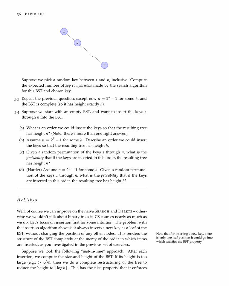
36 david liu
1
2
. . .
n
Suppose we pick a random key between 1 and n, inclusive. Computethe expected number of key comparisons made by the search algorithmfor this BST and chosen key.
3.3 Repeat the previous question, except now n = 2h − 1 for some h, andthe BST is complete (so it has height exactly h).
3.4 Suppose we start with an empty BST, and want to insert the keys 1
through n into the BST.
(a) What is an order we could insert the keys so that the resulting treehas height n? (Note: there’s more than one right answer.)
(b) Assume n = 2h − 1 for some h. Describe an order we could insertthe keys so that the resulting tree has height h.
(c) Given a random permutation of the keys 1 through n, what is theprobability that if the keys are inserted in this order, the resulting treehas height n?
(d) (Harder) Assume n = 2h − 1 for some h. Given a random permuta-tion of the keys 1 through n, what is the probability that if the keysare inserted in this order, the resulting tree has height h?
AVL Trees
Well, of course we can improve on the naïve Search and Delete – other-wise we wouldn’t talk about binary trees in CS courses nearly as much aswe do. Let’s focus on insertion first for some intuition. The problem withthe insertion algorithm above is it always inserts a new key as a leaf of theBST, without changing the position of any other nodes. This renders the Note that for inserting a new key, there
is only one leaf position it could go intowhich satisfies the BST property.
structure of the BST completely at the mercy of the order in which itemsare inserted, as you investigated in the previous set of exercises.
Suppose we took the following “just-in-time” approach. After eachinsertion, we compute the size and height of the BST. If its height is toolarge (e.g., >
√n), then we do a complete restructuring of the tree to
reduce the height to dlog ne. This has the nice property that it enforces

data structures and analysis 37
some maximum limit on the height of the tree, with the downside thatrebalancing an entire tree does not seem so efficient.
You can think of this approach as attempting to maintain an invarianton the data structure – the BST height is roughly log n – but only enforcingthis invariant when it is extremely violated. Sometimes, this does in factlead to efficient data structures, as we’ll study in Chapter 8. However, itturns out that in this case, being stricter with an invariant – enforcing itat every operation – leads to a faster implementation, and this is what wewill focus on for this chapter.
More concretely, we will modify the Insert and Delete algorithmsso that they always perform a check for a particular “balanced” invariant.If this invariant is violated, they perform some minor local restructuringof the tree to restore the invariant. Our goal is to make both the checkand restructuring as simple as possible, to not increase the asymptoticworst-case running times of O(h).
The implementation details for such an approach turn solely on thechoice of invariant we want to preserve. This may sound strange: can’twe just use the invariant “the height of the tree is ≤ dlog ne”? It turnsout that even though this invariant is the optimal in terms of possibleheight, it requires too much work to maintain every time we mutate thetree. Instead, several weaker invariants have been studied and used in the
Such data structures include red-blacktrees and 2-3-4 trees.
decades that BSTs have been studied, and corresponding names coinedfor the different data structures. In this course, we will look at one of thesimpler invariants, used in the data structure known as the AVL tree.
The AVL tree invariant
In a full binary tree (2h − 1 nodes stored in a binary tree of height h),every node has the property that the height of its left subtree is equal tothe height of its right subtree. Even when the binary tree is complete, theheights of the left and right subtrees of any node differ by at most 1. Ournext definitions describe a slightly looser version of this property.
Definition 3.1 (balance factor). The balance factor of a node in a binarytree is the height of its right subtree minus the height of its left subtree.
0
2 -1
-1 -1 0
0 0
Each node is labelled by its balancefactor.
Definition 3.2 (AVL invariant, AVL tree). A node satisfies the AVL invari-ant if its balance factor is between -1 and 1. A binary tree is AVL-balancedif all of its nodes satisfy the AVL invariant.
An AVL tree is a binary search tree which is AVL-balanced.
The balance factor of a node lends itself very well to our style of recur-sive algorithms because it is a local property: it can be checked for a given

38 david liu
node just by looking at the subtree rooted at that node, without knowingabout the rest of the tree. Moreover, if we modify the implementation ofthe binary tree node so that each node maintains its height as an attribute,whether or not a node satisfies the AVL invariant can even be checked inconstant time!
There are two important questions that come out of this invariant:
These can be reframed as, “how muchcomplexity does this invariant add?”and “what does this invariant buy us?”
• How do we preserve this invariant when inserting and deleting nodes?
• How does this invariant affect the height of an AVL tree?
For the second question, the intuition is that if each node’s subtreesare almost the same height, then the whole tree is pretty close to beingcomplete, and so should have small height. We’ll make this more precisea bit later in this chapter. But first, we turn our attention to the morealgorithmic challenge of modifying the naïve BST insertion and deletionalgorithms to preserve the AVL invariant.
Exercise Break!
3.5 Give an algorithm for taking an arbitrary BST of size n and modifyingit so that its height becomes dlog ne, and which runs in time O(n log n).
3.6 Investigate the balance factors for nodes in a complete binary tree. Howmany nodes have a balance factor of 0? -1? 1?
Rotations
As we discussed earlier, our high-level approach is the following:
(i) Perform an insertion/deletion using the old algorithm.
(ii) If any nodes have the balance factor invariant violated, restore the in-variant.
How do we restore the AVL invariant? Before we get into the nitty-gritty details, we first make the following global observation: inserting ordeleting a node can only change the balance factors of its ancestors. This is be-cause inserting/deleting a node can only change the height of the subtreeswhich contain this node, and these subtrees are exactly the ones whoseroots are ancestors of the node. For simplicity, we’ll spend the remainderof this section focused on insertion; AVL deletion can be performed inalmost exactly the same way.

data structures and analysis 39
Even better, the naïve algorithms already traverse exactly the nodeswhich are ancestors of the modified node. So it is extremely straight-forward to check and restore the AVL invariant for these nodes; we cansimply do so after the recursive Insert, Delete, ExtractMax, or Ex-tractMin call. So we go down the tree to search for the correct spot toinsert the node, and then go back up the tree to restore the AVL invari-ant. Our code looks like the following (only Insert is shown; Delete issimilar):
1 def Insert(D, key, value):
2 # Insert the key-value pair into <D>
3 # Same code as before, omitted
4 ...
5
6 # Update the height attribute
7 D.height = max(D.left.height, D.right.height) + 1
8
9 D.balance_factor = D.right.height - D.left.height
10 if D.balance_factor < -1 or D.balance_factor > 1:
11 # Fix the imbalance for the root node.
12 fix_imbalance(D)
Let us spell out what fix_imbalance must do. It gets as input a BSTwhere the root’s balance factor is less than −1 or greater than 1. However,because of the recursive calls to Insert, we can assume that all the non-rootnodes in D satisfy the AVL invariant, which is a big help: all we need to dois fix the root. Reminder here about the power of
recursion: we can assume that therecursive Insert calls worked properlyon the subtree of D, and in particularmade sure that the subtree containingthe new node is an AVL tree.
One other observation is a big help. We can assume that at the begin-ning of every insertion, the tree is already an AVL tree – that it is balanced.Since inserting a node can cause a subtree’s height to increase by at most1, each node’s balance factor can change by at most 1 as well. Thus if theroot does not satisfy the AVL invariant after an insertion, its balance factorcan only be -2 or 2.
These observations together severely limit the “bad cases” for the rootthat we are responsible for fixing. In fact, these restrictions make it quitestraightforward to define a small set of simple, constant-time proceduresto restructure the tree to restore the balance factor in these cases. Theseprocedures are called rotations.

40 david liu
Right rotation
These rotations are best explained through pictures. In the top diagram,variables x and y are keys, while the triangles A, B, and C represent arbi-trary subtrees (that could consist of many nodes). We assume that all thenodes except y satisfy the AVL invariant, and that the balance factor of yis -2.
This means that its left subtree must have height 2 greater than its rightsubtree, and so A.height = C.height + 1 or B.height = C.height + 1. Wewill first consider the case A.height = C.height + 1.
y
x C
A B
x
A y
B C
In this case, we can perform a right rotation to make x the new root,moving around the three subtrees and y as in the second diagram to pre-serve the BST property. It is worth checking carefully that this rotationdoes indeed restore the invariant.
Lemma 3.1 (Correctness of right rotation). Let x, y, A, B, and C be definedas in the margin figure. Assume that this tree is a binary search tree, and that xand every node in A, B, and C satisfy the balance factor invariant. Also assumethat A.height = C.height + 1, and y has a balance factor of -2.
Then applying a right rotation to the tree results in an AVL tree, and in par-ticular, x and y satisfy the AVL invariant.
Proof. First, observe that whether or not a node satisfies the balance factorinvariant only depends on its descendants. Then since the right rotationdoesn’t change the internal structure of A, B, and C, all the nodes in thesesubtrees still satisfy the AVL invariant after the rotation. So we only need This is the power of having a local
property like the balance factor invari-ant. Even though A, B, and C movearound, their contents don’t change.
to show that both x and y satisfy the invariant.
• Node y. The new balance factor of y is C.height− B.height. Since x orig-inally satisfied the balance factor, we know that B.height ≥ A.height−1 = C.height. Moreover, since y originally had a balance factor of−2, we know that B.height ≤ C.height + 1. So B.height = C.heightor B.height = C.height + 1, and the balance factor is either -1 or 0.
• Node x. The new balance factor of x is A.height− (1+max(B.height, C.height)).Our assumption tells us that A.height = C.height + 1, and as we justobserved, either B.height = C.height or B.height = C.height + 1, so thebalance factor of x is also -1 or 0.
Left-right rotation
What about the case when B.height = C.height+ 1 and A.height = C.height?Well, before we get ahead of ourselves, let’s think about what would hap-pen if we just applied the same right rotation as before.

data structures and analysis 41
The diagram looks exactly the same, and in fact the AVL invariant fory still holds. The problem is now the relationship between A.height andB.height: because A.height = C.height = B.height− 1, this rotation wouldleave x with a balance factor of 2. Not good.
Since in this case B is “too tall,” we will break it down further andmove its subtrees separately. Keep in mind that we’re still assuming theAVL invariant is satisfied for every node except the root y.
y
x C
A z
D E
y
z C
x E
A D
z
x y
A D E C
By our assumption, A.height = B.height − 1, and so both D and E’sheights are either A.height or A.height − 1. Now we can first perform aleft rotation rooted at x, which is symmetric to the right rotation we sawabove, except the root’s right child becomes the new root.
This brings us to the situation we had in the first case, where the leftsubtree of z is at least as tall as the right subtree of z. So we do the samething and perform a right rotation rooted at y. Note that we’re treatingthe entire subtree rooted at x as one component here.
Given that we now have two rotations to reason about instead of one, aformal proof of correctness is quite helpful.
Lemma 3.2. Let A, C, D, E, x, y, and z are defined as in the diagram. Assumethat x, z, and every node in A, C, D, E satisfy the AVL invariant. Furthermore,assume the following restrictions on heights, which cause the balance factor of yto be -2, and for the B subtree to have height C.height + 1.
(i) A.height = C.height
(ii) D.height = C.height + 1 or E.height = C.height + 1.
Then after performing a left rotation at x, then a right rotation at y, the result-ing tree is an AVL tree. This combined operation is sometimes called a left-rightdouble rotation.
Proof. As before, because the subtrees A, C, D, and E don’t change theirinternal composition, all their nodes still satisfy the AVL invariant afterthe transformation. We need to check the balance factor for x, y, and z:
• Node x: since x originally satisfied the AVL invariant, D.height ≥A.height. And since the balance factor for y was originally -2, D.height ≤C.height + 1 = A.height + 1. So then the balance factor is either 0 or 1.
• Node y: by assumption (ii), either E.height = C.height+ 1 or D.height =C.height + 1. If E.height = C.height + 1, the balance factor of y is -1.Otherwise, D.height = C.height + 1, and so (since z originally satisfiedthe AVL invariant) E.height = D.height − 1. In this case, the balance E.height 6= D.height + 1, as otherwise
the original balance factor for y wouldbe less than −2.
factor of y is 0.
• Node z: since D.height ≥ A.height, the left subtree’s height is D.height+1. Similarly, the right subtree height is E.height + 1. The balance factor

42 david liu
is then (E.height + 1)− (D.height + 1) = E.height− D.height, which isthe same balance factor as z originally. Since we assumed z originallysatisfied the AVL invariant, z must satisfy the AVL invariant at the endof the rotations.
We leave it as an exercise to think about the cases where the right sub-tree’s height is 2 more than the left subtree’s. The arguments are symmet-ric; the two relevant rotations are “left” and “right-left” rotations.
AVL tree implementation
We now have a strong lemma which tells us that if we take a balancedAVL tree, then perturb its height slightly (by no more than one), we canrearrange the tree in constant time to restore the balanced property. Thisis great for our insertion and deletion algorithms, which only ever changeone node. Here is our full AVL tree Insert algorithm:
You’ll notice that we’ve deliberatelyleft some details to the exercises. Inparticular, we want you to think aboutthe symmetric actions for detecting andfixing an imbalance.
1 def Insert(D, key, value):
2 # Insert the key-value pair into <D>
3 # Same code as before, omitted
4 ...
5
6 # Update the height attribute
7 D.height = max(D.left.height, D.right.height) + 1
8
9 D.balance_factor = D.right.height - D.left.height
10 if D.balance_factor < -1 or D.balance_factor > 1:
11 # Fix the imbalance for the root node.
12 fix_imbalance(D)
13
14
15 def fix_imbalance(D):
16 # Check balance factor and perform rotations
17 if D.balance_factor == -2:
18 if D.left.left.height == D.right.height + 1:
19 right_rotate(D)
20 else: # D.left.right.height == D.right.height + 1
21 left_rotate(D.left)
22 right_rotate(D)
23 elif D.balance_factor == 2:
24 # left as an exercise; symmetric to above case

data structures and analysis 43
25 ...
26
27
28 def right_rotate(D):
29 # Using some temporary variables to match up with the diagram
30 y = D.root
31 x = D.left.root
32 A = D.left.left
33 B = D.left.right
34 C = D.right
35
36 D.root = x
37 D.left = A
38 # Assume access to constructor AVLTree(root, left, right)
39 D.right = AVLTree(y, B, C)
40
41
42 def left_rotate(D):
43 # Left as an exercise
Theorem 3.3 (AVL Tree Correctness). The above AVL Tree insertion algorithmis correct. That is, it results in a binary tree which satisfies the binary search treeproperty and is balanced, with one extra node added, and with the height andbalance_factor attributes set properly.
Proof. Since insertion starts with the naïve algorithm, we know that itcorrectly changes the contents of the tree. We need only to check thatfix_imbalance results in a balanced BST.
Right before fix_imbalance is called in either function, we know that Dstill satisfies the BST property, and that its subtrees are AVL trees (since weassume that the recursive calls correctly restore this property). Moreover,because at most one node has changed in the BST, the balance factor ofthe root is between -2 and 2.
The correctness of fix_imbalance when the root’s balance factor is -2 isdirectly implied by the previous two lemmas. The other case is symmetric,and was left as an exercise. Then we are done, since after fix_imbalance
returns, the tree is an AVL tree – all its nodes satisfy the AVL invariant.
Analysis of AVL Algorithms
In the preceding sections, we put in quite a bit of effort in ensuring thatthe AVL invariant is preserved for every node in the tree. Now, it is timeto reap the benefits of this additional restriction on the structure of the

44 david liu
tree in our running time analysis of the modified Insert and Delete
algorithms.
First, a simple lemma which should look familiar, as it is the basis ofmost recursive tree algorithm analyses.
Lemma 3.4. The worst-case running time of AVL tree insertion and deletion isO(h), the same as for the naïve insertion and deletion algorithms. Don’t forget that we’ve only proved
a O(h) upper bound in these notes –you’re responsible for proving a lowerbound yourself!Proof. We simply observe that the new implemention consists of the old
one, plus the new updates of height and balaned_factor attributes, andat most two rotations. This adds a constant-time overhead per recursivecall, and as before, there are O(h) recursive calls made. So the total run-ning time is still O(h).
So far, the analysis is exactly the same as for naïve BSTs. Here is wherewe diverge to success. As we observed at the beginning of this section,BSTs can be extremely imbalanced, and have height equal to the numberof nodes in the tree. This is obviously not true for AVL trees, whichcannot have all their nodes on (say) the left subtree. But AVL trees are notperfectly balanced, either, since each node’s two subtree heights can differby 1. So the question is, is restricting the balance factor for each node tothe range −1, 0, 1 good enough to get a strong bound on the height ofthe AVL tree? The answer is a satisfying yes.
Lemma 3.5 (AVL Tree Height). An AVL tree with n nodes has height at most1.44 log n.
Proof. It turns out to be easier to answer a question which is inverse to thestatement in the theorem: what is N(h), the minimum number of nodes inan AVL tree of height h? Our goal is to get a tight bound (or exact formula)for N(h). Some playing around quickly yields the following small values:N(0) = 0, N(1) = 1, N(2) = 2, N(3) = 4, N(4) = 7.
Not much of a pattern so far, though drawing pictures is suggestive:an AVL tree of height h with minimum size must have a subtree whichis an AVL tree of height h− 1, and another subtree which is an AVL treeof height h− 2, and both of its subtrees must have minimum size. Herewe’re implicitly using the fact that being balanced, and hence an AVL tree,is a recursive property: the subtrees of an AVL tree are themselves AVLtrees. This gives the following recurrence:
N(h) =
0, h = 0
1, h = 1
N(h− 1) + N(h− 2) + 1, h ≥ 2

data structures and analysis 45
This looks almost, but not quite, the same as the Fibonacci sequence.A bit of trial-and-error or more sophisticated techniques for solving re-currences (beyond the scope of this course) reveal that N(h) = fh+2 − 1,where fi is the i-th Fibonacci number. Since we do have a closed formexpression for the Fibonacci numbers in terms of the golden ratio ϕ =
1 +√
52
, we get the following bound on N(h):
N(h) = fh+2 − 1
> (ϕh+2 − 1)− 1
= ϕh+2 − 2
Recall now the definition of N(h): the minimum number of nodes in anAVL tree of height h. So then if we have n nodes in an AVL tree of heighth, we know that
N(h) ≤ n
ϕh+2 − 2 < n
h < logϕ(n + 2)− 2
h <1
log ϕlog(n + 2)− 2
The theorem follows from calculating1
log ϕ= 1.4404 . . . .
Putting the previous two lemmas together, we can conclude that AVLinsertion, deletion, and search all have logarithmic running time in theworst-case.
Theorem 3.6 (AVL Tree Runtime). AVL tree insertion, deletion, and searchhave worst-case running time Θ(log n), where n is the number of nodes in thetree.
Exercise Break!
3.7 Show that you can use an AVL tree to implement a priority queue.What is an upper bound on the worst-case running time of the threepriority queue operations in this case?


4 Dictionaries, Round Two: Hash Tables
We now look at a completely different approach for implementing dic-tionaries. To get warmed up, consider the following scenario: all of thekey-value pairs we wish to store have keys that are numbers 0 throughK − 1. In this case, we can store these pairs inside an array of lengthK, and achieve constant time search, insertion, and deletion simply bystoring each value at the array index corresponding to its key!
This technique is known as direct addressing, and works well whenthe number of possible keys (and hence total number of pairs) is small.However, array addressing is only constant time if the entire array hasbeen allocated in memory. Thus as K grows larger, even if the runningtime of the dictionary operations stays constant, the space required growslinearly in K. In this chapter, we will study a generalized version of direct This size constraint is infeasible in
many real-world applications of dictio-naries.
addressing known as hashing, which allows us to store key-value pairswhen the keys aren’t necessarily numbers, and using much less spacethan the number of all possible keys.
Hash functions
Let U represent the set of all possible keys we would like to store. Ingeneral, we do not restrict ourselves to just numeric keys, and so U mightbe a set of strings, floating-point numbers, or other custom data types thatwe define based on our application. Like direct addressing, we wish tostore these keys in an array, but here we’ll let the size of the array be aseparate variable m. We won’t assume anything about the relationshipbetween m and |U| right now, though you might already have some ideasabout that.
Definition 4.1 (hash function, hash table). A hash function is a functionh : U → 0, 1, . . . , m− 1. You should think of this as a function that takesa key and computes the array slot where the key is to be placed.
A hash table is a data structure containing an array of length m and ahash function.

48 david liu
1 def Search(hash_table, key):
2 hash = h(key)
3 return hash_table[hash]
4
5 def Insert(hash_table, key, value):
6 hash = h(key)
7 hash_table[hash] = value
8
9 def Delete(hash_table, key):
10 hash = h(key)
11 hash_table[hash] = None
Of course, this is not the end of the story. Even though this imple-mentation is certainly efficient – all three operations run in Θ(1) time – itactually is not guaranteed to be correct.
Remember that we have not made any assumptions about the relation-ship between m, the size of the hash table, and |U|, the total possiblenumber of keys; nor have we said anything about what h actually does.Our current implementation makes the assumption that there are no col-lisions in the hash function, i.e., each key gets mapped to a unique arrayslot. Consider what happens when you try to use the above algorithm toinsert two key-value pairs whose hashed keys are the same index i: thefirst value is stored at index i, but then the second value overwrites it.
Now, if m ≥ |U|, i.e, there are at least as many array slots as possiblekeys, then there always exists a hash function h which has no collisions.Such hash functions are called perfect hash functions, earning the su-perlative name because they enable the above naive hash table implemen-tation to be correct. However, this assumption is often not realistic, as we Of course, even when we know that a
perfect hash function exists for a givenU and m, it is sometimes non-trivial tofind and compute it. Consider the casewhen U is a set of 10 000 names – canyou efficiently implement a perfect hashfunction without storing a sorted list ofthe names?
typically expect the number of possible keys to be extremely large, andthe array to not take up too much space. More concretely, if m < |U|, thenat least one collision is guaranteed to occur, causing the above implemen-tation to fail. The remainder of this chapter will be devoted to discussingtwo strategies for handling collisions.
Closed addressing (“chaining”)
With closed addressing, each array element no longer stores a value asso- this approach is also called “chaining”
ciated with a particular key, but rather a pointer to a linked list of key-valuepairs. Thus, collisions are sidestepped completely by simply insertingboth the key and value into the linked list at the appropriate array index. Why is it necessary to store both the
key and the value?Search and deletion are just slightly more complex, requiring a traversalof the linked list to find the correct key-value pair.

data structures and analysis 49
1 def Search(hash_table, key):
2 hash = h(key)
3 linked_list = hash_table[hash]
4 if linked_list contains key:
5 return corresponding value from linked_list
6 else:
7 return None
8
9 def Insert(hash_table, key, value):
10 hash = h(key)
11 linked_list = hash_table[hash]
12 insert key, value at the head of linked_list
13
14 def Delete(hash_table, key):
15 hash = h(key)
16 linked_list = hash_table[hash]
17 delete key from linked_list
This implementation maintains the invariant that for every key k storedin the table, it must appear in the linked list at position h(k). From thisobservation, we can see that these algorithms are correct. In addition, weonly need to consider the linked list at one particular array index, savinglots of time.
Or perhaps not. What if all of the keys get mapped to the same index?In this case, the worst case of search and deletion reduces to the worst-case search and deletion from a linked list, which is Θ(n), where n is thenumber of pairs stored in the hash table. Can we simply pick a functionthat guarantees that this extreme case won’t happen? Not if we allowthe set of keys to be much larger than the size of the array: for any hashfunction h, there exists an index i such that at least |U|/m keys get mappedto i by h. This type of counting argument is ex-
tremely common in algorithm analysis.If you have a set of numbers whoseaverage is x, then one of the numbersmust have value ≥ x.
So while the worst-case running time for Insert is Θ(1), the worst
Insertions happen at the front of thelinked list
case performance for Search and Insert seems very bad: no better thansimply using a linked list, and much worse than the AVL trees we sawin the previous section. However, it turns out that if we pick good hashfunctions, hash tables with closed addressing are much better than bothof these data structures on average.
Average-case analysis for closed addressing
We will focus on analysing the Search algorithm, whose running timeof course depends on the lengths of the linked lists in the hash table. Delete is basically the same.

50 david liu
Remember that whenever we want to talk about average case, we need todefine a distribution of inputs for the operation. We’ll assume here thatall possible keys are equally likely to be searched for; in other words, we’lluse the uniform distribution on U, and assume n random keys are alreadycontained in the hash table.
However, because the lengths of the linked lists depend on the numberof collisions in our hash function, just knowing the key distribution isn’tenough – for all we know, our hash function could map all keys to thesame index! So we will make an additional assumption known as thesimple uniform hashing assumption, which is that our hash function hsatisfies the property that for all 0 ≤ i < m, the probability that h(k) = i
is1m
, when k is chosen uniformly at random from U. That is, choosing arandom key doesn’t favour one particular index over any other. We willmeasure running time here as the number of keys compared against thesearch input, plus the time for computing the hash function.
First, assume that the key k being searched for is not in the hash table.In this case, the algorithm first computes h(k), and then must traversethe entire linked list stored at index h(k). We’ll assume the first steptakes constant time, and the second step we certainly know takes time More on this later
proportional to the length of the linked list at index h(k). Let T be therunning time of Search on input key k. Then T = 1+ the length of thelinked list stored at h(k), which is equal to the number of the n keys thathash to that particular index. We let L be a random variable representingthe number of keys hashed to h(k). So then T = 1 + L, and so E[T] =1 + E[L]. But by the simple uniform hashing assumption, the probabilitythat each of the n randomly chosen keys already in the hash table have a
hash value of h(k) is1m
, and so E[L] =nm
. This is the well-known expected valuefor a hypergeometric distribution.
So then the average number of keys checked by Search when the key
is not in the hash table is 1 +nm
. The average-case running time is then
Θ(1 +nm). Remember what these variables mean: n is the number of
keys already stored in the hash table, and m is the number of spots in thearray. This running time tells us that if the number of keys is any constantmultiple of the size of the array, then doing a search when the key is notin the hash table is a constant-time operation on average.
What about when the search is successful, i.e., when we search for akey that is already in the hash table? Consider searching for ki, the i-thkey inserted into the hash table. How many keys are checked during thissearch? Since items are inserted at the front of the linked list, the numberof keys searched is equal to the number of keys inserted after ki into thesame index as ki, plus one for examining ki itself. Since n − i keys areinserted after ki, by the simple uniform hashing assumption the expected

data structures and analysis 51
number of keys inserted into h(ki) after ki isn− i
m. So then to compute
the average running time, we add the cost of computing the hash function(just 1 step) plus the average of searching for each ki:
E[T] = 1 +1n
n
∑i=1
expected number of keys visited by search for ki
= 1 +1n
n
∑i=1
(1 +
n− im
)= 2 +
1n
n
∑i=1
nm− 1
n
n
∑i=1
im
= 2 +nm− 1
n· n(n + 1)
2m
= 2 +nm− n + 1
2m
= 2 +n
2m− 1
2m
= Θ(
1 +nm
)The average-case running time for Delete is the same, since once a
key has been found in an array, it is only a constant-time step to removethat node from the linked list.
Because the rationm
between the number of keys stored and the numberof spots in the array comes up frequently in hashing analysis, we give it aspecial name.
Definition 4.2 (load factor). The load factor of a hash table is the ratio ofthe number of keys stored to the size of the table. We use the notation
α =nm
, where n is the number of keys, and m the number of slots.
So we can say that the average-case running time of Search and Delete
are Θ(1 + α).
Exercise Break!
4.1 Suppose that we use an AVL tree instead of a linked list to store thekey-value pairs that are hashed to the same index.
(a) What is the worst-case running time of a search when the hash tablehas n key-value pairs?
(b) What is the average-case running time of an unsuccessful search whenthe hash table has n key-value pairs?

52 david liu
Open addressing
The other strategy used to resolve collisions is to require each array ele-ment to contain only one key, but to allow keys to be mapped to alternateindices when their original spot is already occupied. This saves the spaceoverhead required for storing extra references in the linked lists of closedaddressing, but the cost is that the load factor α must always be less than 1,i.e., the number of keys stored in the hash table cannot exceed the lengthof the array.
In this type of hashing, we have a parameterized hash function h thattakes two arguments, a key and a positive integer. The “first” hash value h : U ×N→ 0, . . . , m− 1for a key k is h(k, 0), and if this spot is occupied, the next index chosen ish(k, 1), and then h(k, 2), etc.
For simplicity, we have omitted abounds check i < m. This would benecessary in practice to ensure thatthis code does not enter into an infiniteloop.
1 def Insert(hash_table, key, value):
2 i = 0
3 while hash_table[h(key, i)] is not None:
4 i = i + 1
5
6 hash_table[h(key, i)].key = key
7 hash_table[h(key, i)].value = value
Searching for an item requires examining not just one spot, but manyspots. Essentially, when searching for a key k, we visit the same sequenceof indices h(k, 0), h(k, 1), etc. until either we find the key, or reach a None
value.
1 def Search(hash_table, key):
2 i = 0
3 while hash_table[h(key, i)] is not None and hash_table[h(key, i)].key != key:
4 i = i + 1
5
6 if hash_table[h(key, i)].key == key:
7 return hash_table[h(key, i)].value
8 else:
9 return None
Deletion seems straightforward – simply search for the given key, thenreplace the item stored in the array with None, right? Not exactly. Supposewe insert a key k into the hash table, but the spot h(k, 0) is occupied, andso this key is stored at index h(k, 1) instead. Then suppose we delete
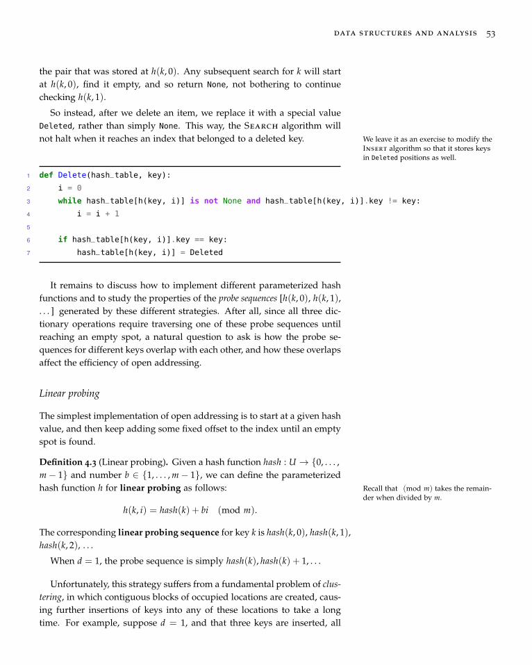
data structures and analysis 53
the pair that was stored at h(k, 0). Any subsequent search for k will startat h(k, 0), find it empty, and so return None, not bothering to continuechecking h(k, 1).
So instead, after we delete an item, we replace it with a special valueDeleted, rather than simply None. This way, the Search algorithm willnot halt when it reaches an index that belonged to a deleted key. We leave it as an exercise to modify the
Insert algorithm so that it stores keysin Deleted positions as well.
1 def Delete(hash_table, key):
2 i = 0
3 while hash_table[h(key, i)] is not None and hash_table[h(key, i)].key != key:
4 i = i + 1
5
6 if hash_table[h(key, i)].key == key:
7 hash_table[h(key, i)] = Deleted
It remains to discuss how to implement different parameterized hashfunctions and to study the properties of the probe sequences [h(k, 0), h(k, 1),. . . ] generated by these different strategies. After all, since all three dic-tionary operations require traversing one of these probe sequences untilreaching an empty spot, a natural question to ask is how the probe se-quences for different keys overlap with each other, and how these overlapsaffect the efficiency of open addressing.
Linear probing
The simplest implementation of open addressing is to start at a given hashvalue, and then keep adding some fixed offset to the index until an emptyspot is found.
Definition 4.3 (Linear probing). Given a hash function hash : U → 0, . . . ,m− 1 and number b ∈ 1, . . . , m− 1, we can define the parameterizedhash function h for linear probing as follows: Recall that (mod m) takes the remain-
der when divided by m.
h(k, i) = hash(k) + bi (mod m).
The corresponding linear probing sequence for key k is hash(k, 0), hash(k, 1),hash(k, 2), . . .
When d = 1, the probe sequence is simply hash(k), hash(k) + 1, . . .
Unfortunately, this strategy suffers from a fundamental problem of clus-tering, in which contiguous blocks of occupied locations are created, caus-ing further insertions of keys into any of these locations to take a longtime. For example, suppose d = 1, and that three keys are inserted, all
54 david liu
with the hash value 10. These will occupy indices 10, 11, and 12 in thehash table. But now any new key with hash value 11 will require 2 spotsto be checked and rejected because they are full. The collision-handlingfor 10 has now ensured that hash values 11 and 12 will also have colli-sions, increasing the runtime for any operation which visits these indices.Moreover, the effect is cumulative: a collision with any index in a clustercauses an extra element to be added at the end of the cluster, growing itin size by one. You’ll study the effects of clustering more precisely in anexercise.
Quadratic probing
The main problem with linear probing is that the hash values in the mid-dle of a cluster will follow the exact same search pattern as a hash valueat the beginning of the cluster. As such, more and more keys are absorbedinto this long search pattern as clusters grow. We can solve this prob-lem using quadratic probing, which causes the offset between consecutiveindices in the probe sequence to increase as the probe sequence is visited.
Definition 4.4 (Quadratic probing). Given a hash function hash : U →0, . . . , m − 1 and numbers b, c ∈ 0, . . . , m − 1, we can define the pa-rameterized hash function h for quadratic probing as follows:
h(k, i) = hash(k) + bi + ci2 (mod m).
Even if a key’s hash value is in the middle of a cluster, it is able to“escape” the cluster much more quickly than using linear probing. How-ever, a form of clustering still occurs: if many items have the same initialhash value, they still follow the exact same probe sequence. For example,if four keys are hashed to the same index, the fourth key inserted mustexamine (and pass) the three indices occupied by the first three keys.
Double hashing
To resolve this problem – a collision in the original hash function causingidentical probe sequences – we change how the offset is calculated so thatit depends on the key being hashed in a particularly clever way.
Definition 4.5 (Double hashing). Given two hash functions hash1, hash2 :U → 0, . . . , m − 1 and number b ∈ 0, . . . , m − 1, we can define theparameterized hash function for double hashing h as follows:
h(k, i) = hash1(k) + b · hash2(k) (mod m).
While both linear and quadratic probing have at most m different probesequences (one for each distinct starting index), this scheme has at most m2
data structures and analysis 55
different probe sequences, one for each pair of values (hash1(k), hash2(k)).Under such a scheme, it is far less likely for large clusters to form: notonly would keys have to have the same initial hash value (using hash1),they would also need to have the same offset (using hash2).
Running time of open addressing
To round out this chapter, we’ll briefly discuss some of the performancecharacteristics of open addressing. First, we observe that there are m!possible probe sequences (i.e., the order in which hash table indices arevisited). A typical simplifying assumption is that the probability of get-ting any one of these sequences is 1/m!, which is not true for any of theprobe sequences studied here – even double hashing has only m2 possiblesequences – but can be a useful approximation.
However, under this assumption, the average number of indices searched
of all three dictionary operations is at most1
1− α. So for example, if the
table is 90% full (so α = 0.9), the average number of indices searchedwould be just 10, which isn’t bad at all!
Exercise Break!
4.2 Suppose we use linear probing with d = 1, and our hash table has nkeys stored in the array indices 0 through n− 1.
(a) What is the maximum number of array indices checked when a keyis searched for in this hash table?
(b) What is the probability that this maximum number of array indicesoccurs? Use the simple uniform hashing assumption.
(c) What is the average running time of Search for this array?

5 Randomized Algorithms
So far, when we have used probability theory to help analyse our algo-rithms we have always done so in the context of average-case analysis: de-fine a probability distribution over the set of possible inputs of a fixedsize, and then calculate the expected running time of the algorithm overthis set of inputs.
This type of analysis is a way of refining our understanding of howquickly an algorithm runs, beyond simply the worst and best possible in-puts, we look at the spread (or distribution) of running times across all dif-ferent inputs. It allows us to say things like “Quicksort may have a worst-case running time of Θ(n), but on average its performance is Θ(n log n),which is the same as mergesort.”
However, average-case analysis has one important limitation: the im-portance of the asymptotic bound is directly correlated with the “plausi-bility” of the probability distribution used to perform the analysis. We cansay, for example, that the average running time of quicksort is Θ(n log n)when the input is a random, uniformly-chosen permutation of n items;but if the input is instead randomly chosen among only the permutationswhich have almost all items sorted, the “average” running time mightbe Θ(n2). We might assume that the keys inserted into a hash table are This assumes naive quicksort which
chooses the first element as the pivot.equally likely to be hashed to any of the m array spots, but if they’re allhashed to the same spot, searching for keys not already in the hash tablewill always take Θ(n) time.
In practice, an algorithm can have an adversarial relationship with theentity feeding it inputs. Not only is there no guarantee that the inputs willhave a distribution close to the one we used in our analysis; a malicioususer could conceivably hand-pick a series of inputs designed to realizethe worst-case running time. That the algorithm has good average-caseperformance means nothing in the face of an onslaught of particularlybad inputs.
In this chapter, we will discuss one particularly powerful algorithmdesign technique which can (sometimes) be used to defend against thisproblem. Rather than assume the randomness exists external to the algo-

58 david liu
rithm in the choice of inputs, this technique makes no assumptions aboutthe input whatsoever, but instead moves the randomness to inside the al-gorithm itself. The key idea is to allow our algorithms to make randomchoices, a departure from the deterministic algorithms – ones which mustfollow a fixed sequence of steps – we have studied so far. Such algorithms,which make random choices as part of their natural execution, are knownas randomized algorithms.
Randomized quicksort
Let us return to quicksort from our first chapter, which we know has poorworst-case performance on pre-sorted lists. Because our implementationalways chooses the first list element as the pivot, a pre-sorted list alwaysresults in maximally uneven partition sizes. We were able to “fix” thisproblem in our average-case analysis with the insight that in a randompermutation, any of the n input numbers is equally likely to be chosen asa pivot in any of the recursive calls to quicksort. You’ll recall our argument was a tad
more subtle and relied on indicatorvariables, but this idea that the pivotwas equally likely to be any numberdid play a central role.
So if we allow our algorithm to make random choices, we can turnany input into a “random” input simply by preprocessing it, and thenapplying the regular quicksort function:
1 def randomized_quicksort(A):
2 randomly permute A
3 quicksort(A)
Huh, this is so simple it almost feels like cheating. The only differenceis the application of a random permutation to the input. The correctnessof this algorithm is clear: because permuting a list doesn’t change itscontents, the exact same items will be sorted, so the output will be thesame. What is more interesting is talking about the running time of this This isn’t entirely true if the list con-
tains duplicates, but there are ways offixing this if we need to.
algorithm.
One important point to note is that for randomized algorithms, the be-haviour of the algorithm depends not only on its input, but also the randomchoices it makes. Thus running a randomized algorithm multiple times onthe same input can lead to different behaviours on each run. In the caseof randomized quicksort, we know that the result – A is sorted – is alwaysthe same. What can change is its running time; after all, it is possible toget as input a “good” input for the original quicksort (sorts in Θ(n log n)time), but then after applying the random permutation the list becomessorted, which is the worst input for quicksort.
In other words, randomly applying a permutation to the input list cancause the running time to increase, decrease, or stay roughly the same.

data structures and analysis 59
So how do we draw conclusions about the running time of randomizedquicksort if we can’t even be certain how long it takes on a single input?Probability, of course!
More precisely, for a fixed input A to randomized quicksort with lengthn, we can define the random variable TA to be the running time of thealgorithm. The main difference between this random variable and theT we used in the average-case analysis of Chapter 1 is that now we areconsidering the probability distribution which the algorithm uses to makeits random choices, and not a probability distribution over inputs. In thecase of randomized quicksort, we would say that the TA random variablehas as its probability space the set of random permutations of 1, . . . , nthe randomized_quicksort algorithm could pick from in its first step.
With this random variable defined, we can now talk about the expectedrunning time of randomized quicksort on the input A, E[TA]. First, whilewe won’t prove it here, it is possible to randomly permute A in O(n) time. See Section 5.3 of CLRS for details.
Applying a random permutation on A results in the standard quicksortrunning on a random permutation of 1, . . . , n as its input, and so theanalysis from Chapter 1 applies, and E[TA] = Θ(n log n).
Warning: students often confuse this type of analysis with the average-case analysis we did earlier in the course. For average-case analysis, wehave a completely deterministic algorithm and a probability distributionover a set of inputs, and are calculating the expected running time acrossthis set of inputs. For this analysis, we have a randomized algorithm anda single input, and are calculating the expected running time across thepossible random choices made by the algorithm itself. You can think about average-case
analysis as putting the randomnessexternal to the algorithm, and random-ized algorithm analysis as keeping therandomness internal to the algorithm.
The work we have done so far is just for one particular input. Let usextend this now to be able to say something about the overall runningtime of the algorithm. We define the worst-case expected running timeof a randomized algorithm to be a function
ET(n) = maxE[Tx] | x is an input of size n.
For randomized quicksort, all lists of size n have the same asymptoticexpected running time, and so we conclude that randomized quicksorthas a worst-case expected running time of Θ(n log n).
You might hear the phrase “worst-case expected” and think this is abit vague: it’s not the “absolute” maximum running time, or even an“average” maximum. So what is this really telling us? The right way tothink about worst-case expected running time is from the perspective ofa malicious user who is trying to feed our algorithm bad inputs. Withregular quicksort, it is possible to give the algorithm an input for whichthe running time is guaranteed to be Θ(n2). However, this is not the casefor randomized quicksort. Here, no matter what input the user picks, if

60 david liu
the algorithm is run many times on this input, the average running timewill be Θ(n log n). Individual runs of randomized quicksort might takelonger, but in the long run our adversary can’t make our algorithm takemore than Θ(n log n) per execution.
Universal Hashing
Now, let us turn to a well-known example of a randomized algorithm:universal hashing. Recall that the simple uniform hashing assumption fromthe previous chapter says that for any array index 0 ≤ i < m, the proba-
bility of choosing a key which hashes to i is1m
. This assumption made the
analysis tractable for us, and in particular ensured a Θ(1+ α) average-caserunning time for the hash table operations. But as we observed, for anyhash function we choose, a simple counting argument tells us that at least|U|/m keys must be hashed to the same index. So if any subset of size nof these keys are inserted, any search for a different key which still hashesto the same index will take Θ(n) time.
To actually do this in practice, a malicious user would study the hashfunction used to determine such a set of colliding keys. You might betempted, then, to keep your hash function a secret so that no one canfigure out these collisions. But a reliance on such an approach only goesso far as how able you (and your colleagues) are in keeping this secret.
But let us take from this the insight that a malicious user needs toknow which hash function is being used in order to purposefully generatelarge numbers of collisions. Rather than keep the hash function a secret,we simply use a set of hash functions, and allow our algorithm to pickrandomly which one to actually use, without making its choice public.To “normal” users, the hash table behaves exactly as expected, regardlessof which hash function is used. In other words, the interface of the hashtable has not changed. But even if a malicious user knows the whole set ofhash functions, she does not know which one is actually being used by thehash table, and in principle cannot determine how to generate collisions.
Of course, if we picked a poor set of hash functions, it might be possiblethat each one has a huge number of collisions, or that the same keys collidefor all or most of the functions. So we certainly need some restriction onthe hash functions which can go into this set, which we make precise inthe following definition.
Definition 5.1 (Universal hash family). Let U be a set of keys, and m ∈ Z+
be the size of the hash table. Let H be a set of hash functions, where eachh ∈ H is a function h : U → 0, . . . , m− 1. We call H a universal hashfamily if and only if for all pairs of distinct keys k1, k2 ∈ U, Note that the probability space is now
the choice of hash functions, and notchoice of keys. This inequality must betrue for every pair of keys!

data structures and analysis 61
Prh∈H[h(k1) = h(k2)] ≤1m
.
Our algorithm is now quite simple. When a new hash table is created,it picks a hash function uniformly at random from a universal hash family,and uses this to do its hashing. This type of hashing is called universalhashing, and is a randomized implementation of hashing commonly usedin practice.
Analysis of universal hashing
Consider a universal hashing scheme which uses closed addressing (chain-ing). We will consider the worst-case expected running time of an unsuccess-ful search for a key k in a hash table storing n keys. Note that this analysisis related to, but distinct from, the analysis we did in the previous chapter.Both are probabilistic, of course, but their probability spaces are different(choose keys vs. choosing hash functions), and the probability assump-tions we are allowed to make are also different, albeit quite similar.
Let h ∈ H be the hash function used by the hash table (chosen uni-formly at random). We want to consider how many of the n keys alreadyin the hash table were inserted into the index h(k), since these keys arethe ones which must be examined in a search for k.
For each inserted key ki, let Xi be the indicator random variable whichis 1 if h(ki) = h(k), and 0 otherwise. We want to compute the expectedsum of these random variables, which we can do nicely using the tech-niques that we’ve seen before. Again, keep in mind that expected valuesand probabilities are over choice of hash function h, not over choice of keys.
E
[n
∑i=1
Xi
]=
n
∑i=1
E[Xi]
=n
∑i=1
Pr[h(ki) = h(k)]
≤n
∑i=1
1m
(universal hash family)
=nm
Note that we have made no assumptions about the keys in the hashtable, nor about k itself: the only property we used was the universal hashfamily property, which gave us the upper bound on the probability thatthe two hash values h(ki) and h(k) were equal. Because this analysis is truefor all possible inputs, we conclude that the worst-case expected runningtime of an unsuccessful search with universal hashing is O(1 + α), where Why didn’t we immediately conclude
Θ(1 + α)?

62 david liu
the 1 comes from computing the hash value of k, as before. A similaranalysis reaches the same asymptotic bound for a successful search.
Constructing a universal hash family
Let us round off our two-chapter discussion of hashing by looking at oneparticular construction of a universal hash family.
We assume that U = 0, 1, . . . , 2w − 1 is the set of natural numberswhich can be stored on a machine word (so typically w = 32 or w = 64),and that m = 2M is a power of two. For every odd number a, 0 < a <
2w, and number (not necessarily odd) b, 0 ≤ b < 2w−M, we define thefollowing hash function:
ha,b(k) = (ak + b mod 2w) // 2w−M.
Note that these functions are very easy to implement; the first computa-tion ak + b mod 2w is simply unsigned integer arithmetic, and the secondoperation is a bit shift, taking the M most significant bits.
While we won’t go into the proof here, it turns out that the set of func-tions ha,b, for the defined ranges on a and b, is a universal hash family.
Exercise Break!
5.1 Prove that the number of hash functions in a universal hash family
must be ≥ 1m
.
5.2 Consider the hash function
h1,0(k) = (k mod 2w) // 2w−M.
Find a set of inputs of size 2w−M which all have the same hash value. This question underlines the factthat an individual hash function ina universal family still has a lot ofcollisions.

6 Graphs
In this chapter, we will study the graph abstract data type, which is oneof the most versatile and fundamental in computer science. You havealready studied trees, which can be used to model hierarchical data likemembers of a family or a classification of living things. Graphs are ageneralization of trees that can represent arbitrary (binary) relationshipsbetween various objects. Some common examples of graphs in practice are There are generalizations of graphs that
model relationships between more thantwo objects at a time, but we won’t gointo that here.
modelling geographic and spatial relationships; activity between membersof a social network; requirements and dependencies in a complex systemlike the development of a space shuttle. By the end of this chapter, you willbe able to define the graph ADT and compare different implementationsof this data type; and perform and analyse algorithms which traversegraphs. If you go on to take CSC373, you
will build on this knowledge to writeand analyse more complex graphalgorithms.
Fundamental graph definitions
As we hinted at in the introduction, a graph is an abstraction of the con-cept of a set of objects and the relationships between them. In the simplestcase, we define a vertex (also called node) v to be a single object, and anedge to be a tuple e = (v1, v2). This is deliberately abstract to be able
to account for a variety of contexts. Forexample, in a social network, you canthink of vertices as people, and edges as“friendships” or “connections.”
Definition 6.1 (graph, undirected/directed). A graph is a tuple of two setsG = (V, E), where V is a set of vertices, and E is a set of edges on thosevertices.
An undirected graph is a graph where order does not matter in theedge tuples: (v1, v2) is equal to (v2, v1). A directed graph is a graph We think of an edge in an undirected
graph as being between two vertices, andan edge in a directed graph as beingfrom a source vertex to a target vertex.
where the tuple order does matter; (v1, v2) and (v2, v1) represent differentedges. In this chapter, if neither type of graph is specified, our default willbe an undirected graph.
There are two obvious measures of a graph’s size: the number of ver-tices and the number of edges. When analysing the running time of graphalgorithms later in this chapter, it will be important to keep in mind howwe are defining “size.”

64 david liu
Before moving on, let’s see some pictures to illustrate some simplegraphs. In each diagram, the vertices are the circles, and the edges arethe lines connecting pairs of circles. Vertices can be labelled or unlabelled,depending on the graph context.
1 2
3
A B
CDa
bc
de
It is clear that there can be a large variation in the characteristics ofgraphs: the number of edges, how many vertices are connected to eachother, how many edges each vertex has, etc. For our purposes, we will Graph theory is a fascinating branch of
mathematics that studies properties ofgraphs such as these, and ones whichare far more complex.
need only a few more definitions to describe some simple graph proper-ties.
Definition 6.2 (adjacent, neighbour). Two vertices are adjacent if there isan edge between them. In this case, we also say that the two vertices areneighbours.
Definition 6.3 (path, length, distance). A path between vertices u and wis a sequence of edges (v0, v1), (v1, v2), . . . , (vk−1, vk), where u = v0 andw = vk, and all the vi are distinct.This follows the English meaning of theterm “path,” where you start at vertex u, take an edge to get to a newvertex v1, take another edge to get to another new vertex v2, and keepfollowing edges until arriving at vk.
The length of the path is the number of edges in the path. For exam-ple, two adjacent vertices are connected by a path of length one, and theprevious notation describes a path of length k. The distance between twovertices is the length of the shortest path between the two vertices. Thedistance between a vertex and itself is always 0.
Paths are fundamental to graphs because they allow us to take basic re-lationships (edges) and derive more complex ones. Suppose, for example,we are representing all the people of the world, with edges representing“A and B personally know each other.” The famous example from socialnetworks is the idea of Six Degrees of Separation, which says that on thisgraph, any two people have a path of length at most 6 between them.Given an arbitrary graph, one might wonder what the maximum pathlength is between any two vertices – or even whether there is a path at all!
Definition 6.4 (connected). We say that a graph is connected if for everypair of vertices in the graph, there is a path between them. Otherwise, wesay the graph is unconnected.

data structures and analysis 65
Implementing graphs
So far, we have discussed graphs as a mathematical abstraction. Our nextstep is to decide how to represent graphs in a program. To be a bit moreconcrete, we define a Graph ADT with two simple operations: obtaininga list of all vertices in the graph, and checking whether two given verticesare adjacent.
Graph ADT
• Vertices(G): Return a list of all the vertices of G.
• CheckAdjacent(G, u, v): Return whether vertices u and v are adjacentin G.
In this section, we’ll consider two implementations of this ADT: ad-jacency lists, which generalize our reference-based tree implementations,and an array-based implementation known as an adjacency matrix.
Adjacency lists
The first approach is one that should be familiar, because it is essentiallywhat we do to implement trees. We use a vertex data type that has a labelattribute to identify the vertex, and a list of references to its neighbours.This latter attribute is known as an adjacency list, from which this imple-mentation gets its name. Since the vertices keep track of the edge data, a In our default undirected case, this
means that two adjacent vertices eachstore a reference to the other in theirrespective adjacency lists.
second graph data type stores only a collection the vertices in the graph.
A common implementation stores thevertices in an array, and labels eachvertex with its array index. If we needto support arbitrary unique identifiers,any dictionary implementation (e.g., ahash table) can be used as well.
To illustrate this approach, we show how one could implement a functionthat checks whether two vertices in a graph are adjacent. Note that thisoperation takes labels, and must use them to look up the correspondingvertices in the graph.
1 def CheckAdjacent(G, i, j):
2 # Access the vertices attribute and perform lookup by labels
3 u = G.vertices[i]
4 v = G.vertices[j]
5 for vertex in u.neighbours:
6 # Note: this assumes labels are unique
7 if vertex.label == v.label:
8 return True
9
10 return False

66 david liu
What is the running time of this algorithm? We assume that lookingup the two vertices in graph.vertices takes constant time, so the running This is true if an array is used; we’ll
leave it as an exercise to think aboutother implementations of this attribute.
time is determined by the number of loop iterations (since the body of theloop always takes constant time). What is an upper bound on the numberof iterations? Well, if there are n vertices in the graph, then u can haveat most n− 1 neighbours (if it has edges going to every other vertex). Itmight be tempting to say O(n) at this point. But remember that there aretwo measures of the size of the graph. If the graph has m edges in total,then m is also an upper bound on the number of neighbours that u canhave. So the number of loop iterations is O(min(m, n)).
For a lower bound, suppose we consider a vertex u that is adjacent tomin(m, n− 1) vertices, and let v be a vertex that is not adjacent to u. Thenperforming this algorithm will cause all min(m, n − 1) iterations of theloop to occur, resulting in a running time of Ω(min(m, n)).
Adjacency matrices
The previous approach was vertex-focused: each vertex is representedas a separate entity in the program, with edges stored implicitly as thereferences in the adjacency lists. It is also possible to represent the edgesdirectly in what we call an adjacency matrix. Suppose there are n verticesin some graph, each with a label between 0 and n− 1. We use an n-by-ntwo-dimensional boolean array, where the ij-entry of the array is true ifthere is an edge between vertex i and vertex j. In the undirected case this matrix is
symmetric across its diagonal, while inthe directed case that’s not guaranteed.Using this approach, determining adjacency in a graph runs in constant
time, since it is just an array lookup:
1 def CheckAdjacent(G, i, j):
2 return G.adjacency[i][j]
Implementation space usage
The adjacency matrix approach seems conceptually simpler and easier toimplement than the adjacency list approach. However, it does have arelatively high space cost, since it must use computer memory to store notonly the edges, but also the “non-edges.” This representation must storea full |V|-by-|V| matrix, with a space cost of Θ(|V|2).
In the adjacency list implementation, the graph itself stores an array ofsize Θ(|V|), and each vertex stores its label and references to its neigh-bours. We cannot count the number of references for an individual vertexbecause that can vary dramatically among vertices in an individual graph.

data structures and analysis 67
But we do have a nice way of calculating the total number of referencesstored across all vertices.
Definition 6.5 (degree). The degree of a vertex is the number of its neigh-bours. For a vertex v, we will usually denote its degree by dv.
Lemma 6.1 (handshake lemma). The sum of the degrees of all vertices is equalto twice the number of edges. Or,
∑v∈V
dv = 2|E|.
This lemma gets its name from thereal-life example of meeting people at aparty. Suppose a bunch of people are ata party always shake hands when theymeet someone new. After greetings aredone, if you ask each person how manynew people they met and add them up,the sum is equal to twice the number ofhandshakes that occurred.
Proof. Each edge e = (u, v) is counted twice in the degree sum: once foru, and once for v.
So this means the total cost of storing the references in our adjacencylist data structure is Θ(|E|), for a total space cost of Θ(|V|+ |E|) (addinga |V| term for storing the labels). Note that this is the cost for storing allthe vertices, not just a single vertex. Adding up the cost for the graph datastructure and all the vertices gives a total space cost of Θ(|V|+ |E|).
At first glance, it may seem that |V|2 and |V|+ |E| are incomparable.However, observe that the maximum number of possible edges is Θ(|V|2),which arises in the case when every vertex is adjacent to every other ver-tex. So in asymptotic terms, |V| + |E| = O(|V|2), but this bound is nottight: if there are very few (e.g., O(|V|)) edges then adjacency lists will bemuch more space efficient than the adjacency matrix.
Graph traversals: breadth-first search
We are now ready to do our first real algorithm on graphs. Consider thecentral problem of exploring a graph by traversing its edges (rather thanrelying on direct access of references or array indices). For example, wemight want to take a social network, and print out the names of everyonewho is connected to a particular person. We would like to be able tostart from a given vertex in a graph, and then visit its neighbours, theneighbours of its neighbours, etc. until we have visited every vertex whichis connected to it. Moreover, we’d like to do so efficiently. If we assume that the graph is con-
nected, then such an exploration visitsevery vertex in the graph.For the next two sections, we will study two approaches for perform-
ing such an exploration in a principled way. The first approach is calledbreadth-first search (BFS). The basic idea is to take a starting vertex s,visit its neighbours, then visit the neighbours of its neighbours, then theneighbours of its neighbours of its neighbours, proceeding until all of thevertices have been explored. The trick is doing so without repeatedly vis-iting the same vertex. To formalize this in an algorithm, we need a way to

68 david liu
keep track of which vertices have already been visited, and which vertexshould be visited next.
To do this, we use a queue as an auxiliary container of pending verticesto be visited. A enqueued attribute is used to keep track of which verticeshave been visited already. This algorithm enqueues the starting vertex,and then repeated dequeues a vertex and enqueues its neighbours whichhaven’t been yet been enqueued.
1 def BFS(graph, s):
2 queue = new empty queue
3 initialize all vertices in the graph to not enqueued
4
5 queue.enqueue(s)
6 s.enqueued = True
7 while queue is not empty:
8 v = queue.dequeue()
9 Visit(v) # do something with v, like print out its label
10
11 for each neighbour u of v:
12 if not u.enqueued:
13 queue.enqueue(u)
A
B
D
C
E
A
B
D
C
E
A
B
D
C
E
A
B
D
C
E
A
B
D
C
E
To illustrate this algorithm, suppose we run it on the graph to the rightstarting at vertex A. We’ll also assume the neighbours are always accessedin alphabetical order. We mark in black when the vertices are visited (i.e.,dequeued and passed to the Visit function).
1. First, A is enqueued. We show this by marking it gray in the diagram.
2. A is dequeued, and its neighbours B and D are stored in the queue.
3. B is visited next, causing its neighbours C and E to be stored on thequeue. Note that A is also B’s neighbour, but it has already been en-queued, and so is not added again.
4. The next vertex to be dequeued is D – remember that we’re storingvertices in a queue, and D was added before C and E. Since D doesn’thave any unvisited neighbours, nothing is added to the queue.
5. The remaining vertices are removed from the queue in the order C thenE.
So the order in which these vertices are visited is A, B, D, C, E.

data structures and analysis 69
Correctness of BFS
Now that we have the algorithm in place, we need to do the two standardthings: show that this algorithm is correct, and analyse its running time.
But what does it mean for breadth-first search to be correct? The in-troductory remarks in this section give some idea, but we need to makethis a little more precise. Remember that we had two goals: to visit everyvertex in the graph, and to visit all the neighbours of the starting vertex,then all of the neighbours of the neighbours, then all of the neighbours ofthe neighbours of the neighbours, etc. We can capture this latter idea byrecalling our definition of distance between vertices. We can then rephrasethe “breadth-first” part of the search to say that we want to visit all ver-tices at distance 1 from the starting vertex, then the vertices at distance 2,then distance 3, etc.
Theorem 6.2 (Correctness of BFS). Let v be the starting vertex chosen by theBFS algorithm. Then for every vertex w which is connected to v, the followingstatements hold:
(1) w is visited. By “visit” here we mean that thefunction Visit is called on the vertex.
(2) Let d be the distance between v and w. Then w is visited after every vertex atdistance at most d− 1 from v.
Proof. We will proceed by induction on the distance between a vertex andv. More formally, let P(n) be the statement that (1) and (2) are true for allvertices with distance n from v.
Base case (P(0)). The only vertex at distance 0 from v is v itself. Then(1) is true because v is certainly visited – it is added to the queue at thebeginning of the algorithm. (2) is vacuously true because there aren’t eventwo distinct vertices to consider.
Inductive step. Let k ≥ 0, and assume P(k) holds. That is, assume allvertices at distance k from v are visited, and visited after all vertices atdistance at most k − 1. If there are no vertices at distance k + 1 from v,then P(k + 1) is vacuously true and we are done.
v
w′
w
...
distance k from v
distance k + 1 from v
Otherwise, let w be a vertex which is at distance k + 1 from v. Then bythe definition of distance, w must have a neighbour w′ which is at distancek from v (w′ is the vertex immediately before w on the path of length kbetween v and w). By the induction hypothesis, w′ is visited. When avertex is visited, all of its neighbours are enqueued into the queue unlessthey have already been enqueued. So w is enqueued. Because the loopdoes not terminate until the queue is empty, this ensures that w at somepoint becomes the current vertex, and hence is visited. This proves thatstatement (1) holds for w.

70 david liu
What about (2)? We need to show that w is visited after every vertex atdistance at most k from v. Let u be a vertex which is at distance d from v,where d ≤ k. Note that d = 0 or d ≥ 1. We’ll only do the d ≥ 1 case here,and leave the other case as an exercise.
By the induction hypothesis, we know that every vertex at distance < dis visited before u. In particular, u has a neighbour u′ at distance d − 1from v which is visited before u. But even more is true: u′ is visited beforew′, since w′ is at distance k from v, and u′ is at distance d− 1 ≤ k− 1 fromv. Then the neighbours of u′, which include u, must be enqueued before This claim uses the induction hypothe-
sis as well.the neighbours of w′, which include w. So u is added to the queue beforew, and hence is dequeued and visited before w. If you read through the proof carefully,
it is only in the last sentence that weuse the fact that we’re storing thevertices in a queue and not some othercollection data type!
Analysis of BFS
Now let us analyse the running time of this algorithm. The creation of thenew queue takes constant time, but the initialization of all vertices to “notenqueued” takes Θ(|V|) time.
The analysis of the loops is a little tricky because it is not immediatelyobvious how many times each loop runs. Let us start with the outerloop, which only terminates when queue is empty. We will do this a bitformally to illustrate the extremely powerful idea that determining theruntime of an algorithm often involves understanding the subtleties ofwhat the algorithm really does.
Proposition 6.3. No vertex is added to the queue more than once.
Proof. Every time a vertex is added to the queue, it is always marked as‘enqueued.’ Only vertices which are not enqueued are ever added to thequeue – the starting vertex is initially unnoticed, and there is an explicitcheck inside the inner loop before enqueuing new vertices. So every vertexis added to the queue at most once.
Proposition 6.4. The outer loop runs for at most |V| times.
Proof. This follows immediately from the previous propostion, and thefact that at each iteration, only one item is dequeued.
Unfortunately, having an upper bound on the number of loop iterationsdoes not immediately give us an upper bound on the program runtime,even if we assume that Visit runs in constant time. The running time ofeach loop iteration depends on the number of times the inner loop runs,which in turn depends on the current vertex.
To tackle the inner loop, you might notice that this is essentially thesame as the space cost analysis for adjacency lists – the inner loop iterates

data structures and analysis 71
once per neighbour of the current vertex. Because we know that curr takeson the value of each vertex at most once, the total number of iterations ofthe inner loop across all vertices is bounded above by the total number of“neighbours” for each vertex. By the Handshake Lemma, this is exactly2 · |E|.
Putting this together yields an upper bound on the worst-case runningtime of O(|V|+ |E|). Is this bound tight? You may think it’s “obvious,”but keep in mind that actually the lower bound doesn’t follow from thearguments we’ve made in this section. The initialization of the vertexenqueued attributes certainly takes Ω(|V|) time, but how do we get a bet-ter lower bound involving |E| using the loops? After all, the first proposi-tion says that each vertex is added at most once. It is conceivable that novertices other than the start are added at all, meaning the loop would onlyrun just once.
This is where our careful analysis of the correctness of the algorithmsaves us. It tells us that every vertex which is connected to the startingvertex is added to the queue and visited. For a lower bound on the worst-case running time, we need a family of inputs (one for each size) whichrun in time Ω(|V| + |E|). Note that the size measure here includes boththe number of vertices and the number of edges. So what kind of inputshould we pick? Well, consider a graph G in which all edges are part of thesame connected component of the graph, and then doing a breadth-first By “connected component” we mean
a group of vertices which are all con-nected to each other.
search starting at one of the vertices in this component.
Then by Theorem 6.2, we know that all vertices in this component arevisited, and the inner loop runs a total of 2 · |E| times (since all edges arebetween vertices in this component). This, combined with the Ω(|V|) timefor initialization, results in an Ω(|V|+ |E|) running time for this family,and hence a lower bound on the worst-case running time of BFS.
Exercise Break!
6.1 Build on our BFS algorithm to visit every vertex in a graph, even if thegraph is not connected. Hint: you’ll need to use a breadth-first searchmore than once.
6.2 Our analysis of BFS assumed that Visit runs in constant time. Let’stry to make this a bit more general: suppose that Visit runs in timeΘ( f (|V|)), where f : N → R+ is some cost function. What is therunning time of BFS in this case?

72 david liu
Graph traversals: depth-first search
We have just finished studing breadth-first search, a graph traversal algo-rithm that prioritizes visiting vertices which are close to the starting vertex.A dual approach is called depth-first search (DFS), which prioritizes visit-ing as many vertices as possible before backtracking to “choose a differentneighbour.” We give a recursive implementation of DFS below. The key Because recursive functions make
great use of the function call stack, thisimplementation is a natural dual of ourqueue-based BFS algorithm.
idea is that a recursive DFS_helper call on a vertex v fully explores the partof the graph reachable from v without revisiting any previously-visitedvertices.
1 def DFS(graph, s):
2 initialize all vertices in the graph to not started or finished
3 DFS_helper(graph, s)
4
5 def DFS_helper(graph, v):
6 v.started = True
7 Visit(v) # do something with v, like print out its label
8
9 for each neighbour u of v:
10 if not u.started:
11 DFS_helper(graph, u)
12
13 v.finished = True
The other major change that we make is that now we have two at-tributes, started and finished, tracking the status of each vertex through-out the search.
• Not started: has not been visited by the search.
• Started but not finished: has been visited by the search, but some ver-tices reachable from this vertex without revisiting other started verticesstill need to be visited.
• Started and finished: it has been has been visited by the search, andall vertices reachable from this vertex without revisiting other startervertices have been visited.

data structures and analysis 73
A
B
D
C
E
A
B C
E
D
A
B C
E
D
A
B C
E
D
A
D
B C
E
A
B
D
C
E
Let us trace through this algorithm on the same graph from the pre-vious section, again starting at vertex A. In the diagram, white verticeshave not been started, gray vertices have been started but not finished,and black vertices have been started and finished.
1. First, A is visited. It is marked as started, but is not yet finished.
2. Then B is visited (A’s first neighbour). It is marked as started.
3. Then C is visited (B’s first neighbour). It is marked as started. Notethat A is not visited again, since it has already been marked as started.
4. Then E is visited (C’s first neighbour). It is marked as started.
5. Since E has no neighbours which haven’t been started, it is marked asfinished, and the recursive call terminates.
6. Similarly, C and B are marked as finished, and their respective recursivecalls terminate, in that order.
7. Control returns to the original search with start A. D is visited (A’ssecond neighbour). It is marked as started.
8. Since D does not have any unvisited neighbours, it is marked as fin-ished. And finally, A is marked as finished as well.
The order in which DFS visits the vertices is A, B, C, E, D.
A note about DFS correctness and runtime
Using a similar analysis as breadth-first search, we are able to prove thefollowing “weak” notion of correctness for depth-first search.
Theorem 6.5 (Weak correctness of DFS). Let v be the starting vertex given asinput the DFS algorithm. Then for every vertex w which is connected to v, thefollowing statement holds:
(1) w is visited.
It is harder to capture the intuitive notion of “depth-first” because thereisn’t an obvious notion of distance to measure. We can, however, formalizethe properties of the attributes started and finished we asserted (withoutproof!) in the previous section.
Theorem 6.6 (Properties of DFS). Suppose DFS_helper is called on a vertex v,and let w be any vertex in the graph which satisfies the following two propertiesat the beginning of the function call:
1. w is not started.

74 david liu
2. There is a path between v and w which consists of only vertices which havenot been started.
Then w is both started and finished when DFS_helper(v) returns.
Finally, using a very similar analysis as BFS, we can obtain the followingtight bound on the worst-case running time of DFS.
Theorem 6.7 (DFS runtime). The worst-case running time of depth-first searchis Θ(|V|+ |E|).
We will leave the proofs of these last two theorems as exercises.
Exercise Break!
6.1 Prove Theorem 6.6.
6.2 Prove Theorem 6.7.
Applications of graph traversals
In this section, we’ll look at two applications of breadth-first and depth-first search that have wide-ranging uses in computer science: detectingcycles in a graph, and determining the shortest path between two vertices.
Detecting cycles (undirected graphs)
Definition 6.6 (cycle). A cycle in a graph is a sequence of distinct edges(v0, v1), (v1, v2), . . . , (vn−1, vn), (vn, v0) which start and end at the samevertex. That is, a cycle is a path which starts
and ends at the same vertex.
Cycles encode a natural “redundancy” in a graph: it is possible to re-move any edge in a cycle without disconnecting its vertices (just take thelong way around the cycle), and so it is often useful to know whether agraph has a cycle, or whether it does not. It turns out that determiningwhether a graph has a cycle or not can be done through a simple mod-ification of either breadth-first or depth-first search, though we will onlyshow the DFS version here.
Recall that depth-first search sets two attributes started and finished
for each vertex, which are used to track the status of the vertex in thesearch. Intuitively, we can use these to detect cycles by checking whetherwe have reached an already-visited node when performing a search. Be-low, we give a modified version of DFS which reports when it detects acycle, with two main changes to the implementation:

data structures and analysis 75
• Each vertex other than the starting vertex stores its parent vertex, whichis the neighbour which caused the vertex to be visited
• The inner loop contains a check for started neighbours that are not theparent of the current vertex; as we’ll show later, this is a valid check fora cycle.
The caveat for our (quite simple) implementation is that it only workswhen the graph is connected; we leave it as an exercise to decide how tomodify it to always report a cycle, even when the graph is is not connected.
1 def DetectCycle(graph):
2 initialize all vertices in the graph to not started or finished
3 s = pick starting vertex
4 DFS_helper(graph, s)
5
6 def DFS_helper(graph, v):
7 v.started = True
8
9 for each neighbour u of v:
10 if not u.started:
11 u.parent = v # NEW: store parent attribute
12 DFS_helper(graph, u)
13 else:
14 # NEW: check for cycle and report
15 if u != v.parent:
16 report that there is a cycle
17
18 v.finished = True
Before we prove the correctness of this algorithm, observe that it is anextremely minor modification of the standard DFS algorithm, and clearlyruns in Θ(|V| + |E|) time. Indeed, a reason cycle detection is a classicapplication of DFS and BFS is that the code changes necessary to solvethis problem add only a constant factor running time overhead to thebasic search algorithms. You could say that the search algorithm does allthe hard work, and cycle detection is thrown in for free.
Of course, one should at least be a little skeptical that minor modifi-cations can be made to an algorithm to solve a different problem. Let usnow prove that this algorithm is indeed correct. You may find it helpfulto review Theorem 6.6 before continuing.
Theorem 6.8 (Cycle Detection with DFS correctness). The modified DFSalgorithm reports that a cycle exists if and only if the input graph has a cycle.

76 david liu
Proof. Let us do the forward direction: assume that the algorithm reportsa cycle. We want to prove that the input graph has a cycle.
Let u and v represent the values of the variables u and v when the cycleis reported. We will claim that u and v are part of a cycle. Note that u andv are neighbours, so all we need to do is show that there is a path from uto v which doesn’t use this edge. We can “close” the path with the edge
to form the cycle.First, since u is started, it must have been visited before v. Let s be the
starting vertex of the DFS. Because both u and v have been visited, theyare both connected to s.
Then there are two possible cases:
• If u is finished, then the path between u and s taken by the DFS doesnot share any vertices in common with the path between v and s otherthan s itself. We can simply join those two paths to get a path betweenv and u.
• If u is not finished, then it must be on the path between v and s. More-over, because it is not the parent of v, the segment of this path betweenu and v contains at least one other vertex, and does not contain theedge (u, v).
Since in both cases we can find a path between u and v not using theedge (u, v), this gives us a cycle.
Now the backwards direction: assume the input graph has a cycle. Wewant to show that a cycle is reported by this algorithm. Let u be the firstvertex in the cycle which is visited by the DFS, and let w be the next vertexin the cycle which is visited.
Though there may be other vertices visited by the search between u andw, we will ignore those, looking only at the vertices on the cycle. Whenw is visited, it and u are the only vertices on the cycle which have beenvisited. In particular, this means that u has at least one neighbour in thecycle which hasn’t been visited. Let v be a neighbour of u which has not This is true even if w and u are neigh-
bours, since u has two neighbours onthe cycle.
yet been visited. Then because there is a path between w and v consistingof vertices which are not started, v must be visited before the DFS_helper
call ends.
Now consider what happens when DFS_helper is called on v. We knowthat u is a neighbour of v, that it is started, and that it is not the parent ofv (since the DFS_helper call on w hasn’t ended yet). Then the conditionsare all met for the algorithm to report the cycle.
Detecting cycles (directed graphs)
Before moving onto our next example, let us take a brief detour into theworld of directed graphs. Recall that a directed graph is one where each

data structures and analysis 77
edge has a direction: the tuple (u, v) represents an edge from u to v, andis treated as different from the edge (v, u) from v to u.
Cycle detection in the directed graphs has several applications; here isjust one example. Consider a directed graph where each vertex is a courseoffered by the University of Toronto, and an edge (u, v) represents therelationship “u is a prerequisite of v.” Then a cycle of three directed edgeswith vertex sequence v1, v2, v3, v1 would represent the relationships “v1 isa prerequisite of v2, v2 is a prerequisite of v3, and v3 is a prerequisite ofv1.” But this is nonsensical: none of the three courses v1, v2, or v3 couldever be taken. Detecting cycles in a prerequisite graph is a vital step toensuring the correctness of this graph.
It turns out that essentially the same algorithm works in both the undi-rected and directed graph case, with one minor modification in the checkfor a cycle. Before we write the algorithm, we note the following changesin terminology in the directed case:
• A neighbour of v is another vertex u such that there is an edge from v tou.
• A directed cycle can have length 2: if there are two vertices u and v suchthat there is an edge from u to v and one from v to u, these two verticesform a cycle. Recall that this was a special case we
had to check for with the “parent”attribute in the undirected case.
1 def DetectCycleDirected(graph):
2 initialize all vertices in the graph to not started or finished
3 s = pick starting vertex
4 DFS_helper(graph, s)
5
6 def DFS_helper(graph, v):
7 v.started = True
8
9 for each neighbour u of v:
10 if not u.started:
11 DFS_helper(graph, u)
12 else:
13 # NEW: check for directed cycle and report
14 if not u.finished:
15 report that there is a cycle
16
17 v.finished = True
We won’t prove the correctness of this algorithm here, as the proof isquite similar to that of the undirected case. It truly is a testament to the

78 david liu
flexibility of DFS that such minor modifications can have such interestingconsequences.
Shortest Path
Let us now turn our attention to a second application of these searches.Recall that BFS visits vertices in order of their distance from the startingvertex. From this information alone, however, we cannot determine pre-cisely how far away a given vertex is from the start. However, if we adaptthe “storing parent” idea to the breadth-first search algorithm, it turns outthat we can not only get the distance between the starting vertex and anarbitrary vertex visited by the search, but also the most direct route as well.
More concretely, suppose we are given a graph and two vertices v andu, and want to find a shortest path between them. Our algorithm is quite Note that there could be multiple paths
of the same minimum length betweenu and v, and we’re only looking for oneof them.
straightforward:
1. Perform a BFS starting at v, storing the parent of each vertex. Here,parent has the same meaning as DFS: the parent of a vertex w is thevertex which, when visited by BFS, causes w to be added to the queue.
2. Return the path formed by starting at u, and following the parent vertexreferences until v is reached. What can we conclude if u’s parent
attribute is unset after the BFS?
Let us formally prove that this algorithm is correct.
Theorem 6.9. Let v be the starting vertex of a BFS on a given graph, and u beany vertex which is connected to v, and d be the distance between u and v.Letu0 = u, u1 be the parent of u0, and in general for all 1 ≤ i ≤ d, ui the parent ofui−1. Then we claim that ud = v, i.e., the path on the vertices u0, u1, . . . , ud oflength d does in fact reach v, making this path one of the shortest possible length.
Proof. We prove this by induction on d, the distance from u to v.
Base case: d = 0. In this case, u must equal v. Then the u0 = u = v, andso the theorem holds in this case. Note that the “shortest path” consistsof just the single vertex v, and has length 0.
Inductive step: suppose the statement holds for some distance d ≥ 0;that is, for every vertex at distance d from v, the path obtained by startingat that vertex and following the parent links d times correctly ends at v.Let u be a vertex which is at distance d + 1 from v. We want to prove thatthe same is true for u (following the parent d + 1 times joins u to v).
Because u is connected to v, it must be visited by the BFS starting at v,and so have a parent. Let u′ be the parent of u. We claim that u′ musthave distance d from v.
First, u′ cannot be at distance < d from v, because otherwise u wouldbe at distance < d + 1 from v. But also u′ cannot be at distance ≥ d + 1

data structures and analysis 79
from v, because then it wouldn’t be the parent of u. Why not? u must havea neighbour of distance d from v, and by the BFS correctness theorem, thisneighbour would be visited before u′ if u′ were at a greater distance fromv. But the parent of u is the first of its neighbours to be visited by BFS, sou′ must be visited before any other of u’s neighbours
So, u′ is at distance d from v. By the induction hypothesis, the sequenceof parents u0 = u′, u1, . . . , ud is a path of length d which ends at v. Butthen the sequence of parents starting at u of length d+ 1 is u, u0, u1, . . . , ud,which also ends at v.
So with this slight modification to breadth-first search, we are able tocompute the shortest path between any two vertices in a graph. Thishas many applications in computer science, including computing efficientroutes for transmitting physical goods and electronic data in a networkand the analysis of dependency graphs of large-scale systems.
Weighted graphs
The story of shortest paths does not end here. Often in real-world ap-plications of graphs, not all edges – relationships – are made equal. Forexample, suppose we have a map of cities and roads between them. Whentrying to find the shortest path between two cities, we do not care aboutthe number of roads that must be taken, but rather the total length acrossall the roads. But so far, our graphs can only represent the fact that twocities are connected by a road, and not how long each road is. To solve thismore general problem, we need to augment our representation of graphsto add such “metadata” to each edge in a graph.
Definition 6.7 (weighted graph, edge weight). A weighted graph is agraph G = (V, E), where each edge now is a triple (v1, v2, w), wherev1, v2 ∈ V are vertices as before, and w ∈ R is a real number called theweight of the edge. Given an edge e, we will use the notation we to referto its weight.
We will refer to our previous graphs with no weights as unweightedgraphs, and that is our default (just like undirected graphs are our default).
Fun fact: you can think of an un-weighted graphs as a weighted graphwhere each edge has weight 1.
The weighted shortest path problem for a weighted graph does not min-imize the number of edges in a path, but instead minimizes the sum ofthe weights along the edges of a path. This is a more complex situationwhich cannot be solved by breadth-first search, and beyond the scope ofthis course. But fear not: you’ll study algorithms for solving this problemin CSC373.

80 david liu
Minimum spanning trees
Now that we have introduced weighted graphs, we will study one morefundamental weighted graph problem in this chapter. Suppose we havea connected weighted graph, and want to remove some edges from thegraph but keep the graph connected. You can think of this as taking a setof roads connecting cities, and removing some the roads while still makingsure that it is possible to get from any city to any other city. Essentially,we want to remove “redundant” edges, the ones whose removal does notdisconnect the graph.
How do we know if such redundant edges exist? It turns out (thoughwe will not prove it here) that if a connected graph has a cycle, thenremoving any edge from that cycle keeps the graph connected. Moreover,if the graph has no cycles, then it does not have any redundant edges. We won’t prove this here, but please
take a course on graph theory if youinterested in exploring more propertieslike this in greater detail.
This property – not having any cycles – is important enough to warrant adefinition.
Definition 6.8 (tree). A tree is a connected graph which has no cycles. Warning: one difference between thisdefinition of tree and the trees you areused to seeing as data structures is thatthe latter are rooted, meaning we giveone vertex special status as the root ofthe tree. This is not the case for trees ingeneral.
So you can view our goal as taking a connected graph, and identifyinga subset of the edges to keep, which results in a tree on the vertices of theoriginal graph.
It turns out that the unweighted case is not very interesting, becauseall trees obey a simple relationship between their number of edges andvertices: every tree with n vertices has exactly n− 1 edges. So finding sucha tree can be done quite easily by repeatedly finding cycles and choosingto keep all but one of the edges.
However, the weighted case is more challenging, and is the problem ofstudy in this section.
Definition 6.9 (minimum spanning tree). The Minimum Spanning TreeProblem takes as input a connected weighted graph G = (V, E), andoutputs a set of edges E′ such that the graph (V, E′) is a tree, and whichminimizes the sum of the weights ∑
e∈E′we. We call such the resulting tree
a minimum spanning tree (MST) of G. As with shortest paths, there might bemore than one minimum spanning treeof G. We just want to find one.
Prim’s algorithm
The first algorithm we will study for solving this problem is known asPrim’s algorithm. The basic idea of this algorithm is quite straightfor-ward: pick a starting vertex for the tree, and then repeatedly add newvertices to the tree, each time selecting an edge with minimum weightwhich connects the current tree to a new vertex.

data structures and analysis 81
1 def PrimMST(G):
2 v = pick starting vertex from G.vertices
3 TV = v # MST vertices
4 TE = # MST edges
5
6 while TV != G.vertices:
7 extensions = (u, v) in G.edges where exactly one of u, v are in TV
8 e = edge in extensions having minimum weight
9 TV = TV + endpoints of e
10 TE = TE + e
11
12 return TE
This algorithm is quite remarkable for two reasons. The first is thatit works regardless of which starting vertex is chosen; in other words,there is no such thing as the “best” starting vertex for this algorithm.The second is that it works without ever backtracking and discarding analready-selected edge to choose a different one. Let us spend some time This algorithm doesn’t “make mistakes”
when choosing edges.studying the algorithm to prove that it is indeed correct.
Theorem 6.10 (Correctness of Prim’s algorithm). Let G = (V, E) be a con-nected, weighted graph. Then Prim’s algorithm returns a set of edges E′ such that(V, E′) is a minimum spanning tree for G.
Proof. The proof of correctness of Prim’s algorithm is an interesting one,because it relies on two loop invariants, one of which is straightforward,but the other of which is very neat and unexpected if you haven’t seenanything like it before. Here are our two invariants (remember that theseare true at the beginning and end of every iteration of the loop):
(1) The graph (TV, TE) is a tree. Remember: trees are connected andhave no cycles.
(2) The tree (TV, TE) can be extended by only adding some edges and ver-tices to a minimum spanning tree of G. This is like saying that TE is a subset of
a possible solution to this problem.
Before we prove that these invariants are correct, let’s see why theyimply the correctness of Prim’s algorithm. When the loop terminates, bothof these invariants hold, so the graph (TV, TE) is a tree and can be extendedto an MST for the input graph. However, when the loop terminates, itscondition is false, and so TV contains all the vertices in the graph. Thismeans that (TV, TE) must be an MST for the input graph, since no morevertices/edges can be added to extend it into one.
We will omit the proof of the first invariant, which is rather straight-forward. The second one is significantly more interesting, and harder to High level: every time a vertex is
added, an edge connecting that ver-tex to the current tree is also added.Adding this edge doesn’t create a cycle.

82 david liu
reason about. Fix a loop iteration. Let (V1, E1) be the tree at the begin-ning of the loop body, and (V2, E2) be the tree at the end of the loop body.We assume that (V1, E1) can be extended to an MST (V, E′) for the input,where E1 ⊆ E′. Our goal is to show that (V2, E2) can still be extended to This assumption is precisely the loop
invariant being true at the beginning ofthe loop body.
an MST for the input (but not necessarily the same one).
What the loop body does is add one vertex v to V1 and one edge e =
(v, u, we) to E1, where u is already in V1, and we is the weight of this edge.So we have V2 = V1 ∪ v and E2 = E1 ∪ e.
Case 1: e ∈ E′. In this case, E2 ⊆ E′, so the tree (V2, E2) can also beextended to the same MST as (V1, E1), so the statement holds.
Case 2: e /∈ E′. This is tougher because this means E2 cannot simplybe extended to E′; we need to find a different minimum spanning tree(V, E′′) which contains E2.
Let us study the minimum spanning tree (V, E′) more carefully. Con-sider the partition of vertices V1, V\V1, in this MST. Let u and v be theendpoints of e; then they must be connected in the MST, and so there is apath between them. Let e′ ∈ E′ be the edge on this path which connects avertex from V1 to a vertex from V\V1. Since e /∈ E′, this means that e′ 6= e.
Now consider what happens in the loop body. Since e′ connects a vertexin V1 to a vertex not in V1, it is put into the set extensions. We also knowthat e was selected as the minimum-weight edge from extensions, and sowe′ ≥ we. Note that their weights could be equal.
Now define the edge set E′′ to be the same as E′, except with e′ removedand e added. The resulting graph (V, E′′) is still connected, and doesn’tcontain any cycles – it is a tree. Moreover, the total weight of its edges isless than or equal to that of E′, since we′ ≥ we. Then the graph (V, E′′) is In fact, because E′ forms a minimum
spanning tree, the total weight ofE′′ can’t be smaller than E′, so theirweights are equal.
also a minimum spanning tree of the input graph, and E ⊆ E′′.
The idea of replacing e′ by e in the initial MST to form a new MST isa very nice one. Intuitively, we argued that at the loop iteration wherewe “should” have chosen e′ to go into the MST, choosing e instead wasstill just as good, and also leads to a correct solution. It is precisely thisargument that “every choice leads to a correct solution” that allows Prim’salgorithm to never backtrack, undoing a choice to make a different one.This has significant efficiency implications, as we’ll study in the next sec-tion.
Analysis of Prim’s algorithm
What is the running time of Prim’s algorithm? Let n be the number ofvertices in the graph, and m be the number of edges. We know that theouter loop always runs exactly n times, each iteration adds one new vertex

data structures and analysis 83
to the set TE, terminating only when TE contains all n vertices. But whathappens inside the loop body?
This is actually where the choice of data structures is important. Notethat we have two sets here, a set of vertices and a set of edges. We’ll firstuse an array to represent these sets, so looking up a particular item oradding a new item takes constant time.
How do we compute extensions, the edges which have one endpointin TV and one endpoint not? We can loop through all the edges, each timechecking its endpoints; this takes Θ(m) time. What about computing the Using adjacency lists, this statement
is certainly true, but requires a bit ofthought. We leave this as an exercise.
minimum weight edge? This is linear in the size of extensions, and so inthe worst case is Θ(m).
This leads to a total running time of Θ(mn), which is not great (recallthat BFS and DFS both took time which was linear in the two quantities,Θ(n + m)). The key inefficiency here is that the inner computations offinding “extension” edges and finding the minimum weight one both doa lot of repeated work in different iterations of the outer loop. After all,from one iteration to the next, the extensions only change slightly, sincethe set TV only changes by one vertex.
So rather than recompute extensions at every iteration, we maintain aheap of edges which extend the current tree (TV, TE), where the “priority”of an edge is simply its weight. This is quite nice because the operation wewant to perform on extensions, find the edge with the minimum weight,is well-suited to what heaps can give us.
So we can rearrange our loop to check each edge exactly once, providedwe do some pre-sorting on the edges to make sure that when each edge ischecked, it is has the minimum weight of all the remaining edges. Sincewe only care about getting the remaining edge with the minimum weight,this is a perfect time for a heap:
1 def PrimMST(G):
2 v = pick starting vertex from G.vertices
3 TV = v # MST vertices
4 TE = # MST edges
5 extensions = new heap # treat weights as priority
6 for each edge on v:
7 Insert(extensions, edge)
8
9 while TV != G.vertices:
10 e = ExtractMin(extensions)
11 u = endpoint of e not in TV
12
13 TV = TV + u

84 david liu
14 TE = TE + e
15 for each edge on u:
16 if other endpoint of edge is not in TV:
17 Insert(extensions, edge)
18
19 return TE
We will do an informal running time analysis of this algorithm. First,we note that each edge is added to the heap at most once, and so the totalnumber of calls to Insert is O(|E|). This means that the cost of all theheap operations (both Insert as well as ExtractMax) take O(|E| log |E|) intotal.
At each iteration, the endpoints of the extracted edge much be checkedfor membership in TV. A naïve implementation of this would search ev-ery element of TV, for a worst-case running time of Θ(|V|). This can beimproved by two methods: store an attribute for each vertex indicatingwhether it is currently in TV or not, or use an AVL tree or hash table tostore the set to support asymptotically faster lookup. We will assumewe’re using the first approach, which reduces the check to a constant-timeoperation.
Since all the other operations take constant time, the running time isO(|E| log |E|+ |V|) = O(|E| log |E|), since |E| ≥ |V| − 1 for a connectedgraph. It turns out that with a bit more effort, we can get this down toO(|V| log |V|) – see CLRS, section 23.2 for details.
Kruskal’s algorithm
As a bridge between this chapter and our next major topic of discussion,we will look at another algorithm for solving the minimum spanning treeproblem. You might wonder why we need another algorithm at all: didn’twe just spend a lot of time developing an algorithm that seems to workperfectly well? But of course, there are plenty of reasons to study morethan one algorithm for solving a given problem, much as there is forstudying more than one implementation of a given ADT: generation ofnew ideas or insights into problem structure; improving running time ef-ficiency; different possible directions of generalization. In this particularcase, we have a pedagogical reason for introducing this algorithm here aswell, as motivation for the final abstract data type we will study in thiscourse.
The second algorithm for solving the minimum spanning tree problemis known as Kruskal’s algorithm. It is quite similar to Prim’s algorithm,in that it incrementally builds up an MST by selecting “good” edges oneat a time. Rather than build up a single connected component of vertices,

data structures and analysis 85
however, it simply sorts edges by weight, and always picks the smallest-weight edge it can without creating a cycle with the edges which havealready been selected.
1 def KruskalMST(G):
2 TE =
3 sort G.edges in non-decreasing order of weights
4
5 for e in G.edges: # starting with the smallest weight edge
6 if TE + e does not have a cycle:
7 TE = TE + e
8
9 return TE
We will omit the proof of correctness of Kruskal’s algorithm, although itis quite remarkable that this algorithm works correctly given its simplicity.
The running time of this algorithm is more interesting. The sortingof edges takes Θ(|E| log |E|) in the worst-case and the outer loop runs atmost |E| times. The really interesting part of the algorithm comes fromchecking whether adding a new edge e to TE creates a cycle or not. Anatural approach is to use what we learned earlier in this chapter andperform either a depth-first or breadth-first search starting from one ofthe endpoints of the chosen edge, using only the edges in TE + e. Thisis rather inefficient, since the O(|V| + |E|) running time of the search isrepeated O(|E|) times, for a total running time of O(|E| log |E|+ |E|(|V|+|E|)) = O(|E| · |V|+ |E|2). Well, this is at least the obvious upper
bound calculation. We leave it as anexercise to prove a tight lower bound onthe worst-case running time.
However, there is a much smarter way of checking whether addinga given edge creates a cycle or not, by keeping track of the connectedcomponents of the vertices defined by the edges in TE. At the beginning ofKruskal’s algorithm, we can view each vertex as being its own component,since TE is empty. When the first edge is added, its two endpoints aremerged into the same component. As more and more edges are added,components merge together, until eventually there is only one component,the minimum spanning tree.
How does this help checking whether adding an edge creates a cycle ornot? We look at the two endpoints of the new edge: if they are in the sameconnected component, then adding the edge creates a cycle; otherwise,adding an edge doesn’t create a cycle, and causes the two components ofits endpoints to be merged.

86 david liu
1 def KruskalMST(G):
2 TE =
3 sort G.edges in non-decreasing order of weights
4 set each vertex to be its own connected component
5
6 for e in G.edges: # starting with the smallest weight edge
7 if the endpoints of e are not in the same connected component:
8 TE = TE + e
9 merge the connected components containing the endpoints of e
The running time of the algorithm now depends on how quickly wecan maintain these components while performing these three operations:
• create a new component for each vertex
• determine whether two vertices are in the same component
• merge two components together
As we will see in the following two chapters, the answer is: “we cansupport all three of these operations very efficiently, if we consider theoperations in bulk rather than one at a time.” But before we formalize theabstract data type to support these operations and study some implemen-tations of this data type, we need to really understand what it means to“consider the operations in bulk.” This is a type of runtime analysis dis-tinct from worst-case, average-case, and even worst-case expected runningtimes, and is the topic of the next chapter.

7 Amortized Analysis
In this chapter, we will study another form of algorithm analysis thatoffers a new type of refinement of worst-case analysis. To set the stagefor this technique, let us recall the context of hash tables from Chapter 4.Recall recall that in hashing with open addressing, keys are stored directlyin the table itself, with collisions being resolved by iterating through aprobe sequence of possible indices until an unoccupied spot is found. Whenwe considered hashing with open addressing (probe sequences), we hadan underlying assumption that there would be space for every new key-value pair inserted (as long as you probed long enough). This impliedthat the array used to store the pairs was bigger than the number of pairsstored. In general, however, we do not know a priori how many pairs aregoing to be stored in the hash table, and so it is impossible to predict howlarge an array to use.
One can get around this problem by storing the hash table with a datastructure which uses dynamically-allocated memory like a linked list orAVL tree, but then we lose the constant-time addressing feature that weget from storing items in a contiguous block of memory. In this chapter,we will study a variant of arrays called dynamic arrays, which we useto implement a resizable collection of items which supports constant-timeaddressing, and “efficient” insertion of new items. We put efficient inquotation marks here because our standard measures of efficiency eitherwon’t apply or won’t be impressive. Instead, we will define and justify anew type of running time analysis for which dynamic arrays are excellentknown as amortized analysis.
Dynamic arrays
The idea of a dynamic array is to keep the fundamental array propertyof storing items in a contiguous memory block, but allow the array toexpand when the existing array is full. One might think that this is atrivial problem, as we can always increase the size of an array by givingit ownership of some memory blocks after its current endpoint. But of

88 david liu
course that memory might be already allocated for a different use, and if This “different use” might even beexternal to our program altogether!it is then the existing array cannot simply be expanded.
Instead, we will do the only thing we can, and allocate a separate andbigger block of memory for the array, copying over all existing elements,and then inserting the new element. We show below one basic imple-mentation of this approach, where A is a wrapper around an array whichhas been augmented with three attributes: array, a reference to the ac-tual array, allocated, the total amount of memory allocated for this array,and size, the number of filled spots in A. For this implementation, wechoose an “expansion factor” of two, meaning that each time the array isexpanded, the memory block allocated doubles in size.
1 def insert(A, x):
2 # Check whether current array is full
3 if A.size == A.allocated:
4 new_array = new array of length (A.allocated * 2)
5 copy all elements of A.array into new_array
6 A.array = new_array
7 A.allocated = A.allocated * 2
8
9 # insert the new element into the first empty spot
10 A.array[A.size] = x
11 A.size = A.size + 1
Worst-case running time of dynamic arrays
For the purposes of analysing the running time of this data structure, wewill only count the number of array accesses made. This actually allowsus to compute an exact number for the cost, which will be useful in thefollowing sections. While this does cause us to ignore the
cost of the other operations, all of themare constant time, and so focusing onthe number of array accesses won’taffect our asymptotic analysis.
For now, suppose we have a dynamic array which contains n items.We note that the final two steps involve just one array access (insertingthe new item x), while the code executed in the if block has exactly 2naccesses: access each of the n items in the old array and copy the value tothe new array.
So we have a worst-case running time of 2n + 1 = O(n) array accesses.This upper bound does not seem very impressive: AVL trees were able tosupport insertion in worst-case Θ(log n) time, for instance. So why shouldwe bother with dynamic arrays at all? The intuition is that this linearworst-case insertion is not a truly representative measure of the efficiencyof this algorithm, since it only occurs when the array is full. Furthermore,if we assume the array length starts at 1 and doubles each time the array

data structures and analysis 89
expands, the array lengths are always powers of 2. This means that 2n + 1array accesses can only ever occur when n is a power of 2; the rest of thetime, insertion accesses only a single element! A bit more formally, if T(n)is the number of array accesses when inserting into a dynamic array withn items, then
T(n) =
2n + 1, if n is a power of 2
1, otherwise
So while it is true that T(n) = O(n), it is not true that T(n) = Θ(n).
Are average-case or worst-case expected analyses any better here? Well,remember that these forms of analysis are only relevant if we treat eitherthe input data as random, or if the algorithm itself has some randomness.This algorithm certainly doesn’t have any randomness in it, and there isn’ta realistic input distribution (over a finite set of inputs) we can use here,as the whole point of this application is to be able to handle insertion intoarrays of any length. So what do we do instead?
Amortized analysis
Before we give a formal definition of amortized analysis, let us expandon one important detail from our informal discussion in the previous sec-tion. We observed that dynamic array insertion was only very rarely slow(when the number of items is a power of two and the array is full), withany other situation being extremely fast. But even more is true: the onlyway to reach the “bad” state of inserting into a full array is by first per-forming a series of (mostly fast) insertions.
Consider inserting an item into a full array of allocated length 210 =
1024. Since 1024 is a power of two, we know that this will take 2049
array accesses. However, to even reach such a state, we must have firsttaken an array of length 512, expanded it to an array length 1024, andthen performed 511 insertions to fill up the expanded array. And these Remember that the expansion is caused
when a new item is inserted, so the ex-panded array starts with 513 elements.
511 insertions would each have taken just one array access each!
So we can contextualize the “inefficient” insertion into the full 1024-length array by noting that it must have been preceded by 511 extremelyefficient insertions, which doesn’t sound so bad.
More formally, an amortized analysis of a data structure computes themaximum possible average cost per operation in a sequence of operations, start-ing from some initial base state. Unlike both worst- and average-case anal- You can ignore the “maximum possi-
ble” for now, since for dynamic arrayswe only have one possible operation– insertion – and hence one possiblesequence of operations.
yses, we are not concerned here with studying one individual operation,but rather the total cost of a sequence of operations performed on a datastructure, and relating this to the number of operations performed. Before

90 david liu
we discuss methods of performing this type of analysis, it is important tokeep in mind that there are two different ways of thinking about the amor-tized cost of a set of operations:
• The average cost of an operation when multiple operations are per-formed in a row. Note that this is a different use of “average” thanaverage-case analysis, which considers an operation as an isolated event,but allows for consideration of multiple inputs.
• The total cost of a sequence of m operations as a function of m. Notethat a sequence of m constant-time operations must have a total runningtime of Θ(m), so expressions that look “linear” aren’t directly referenc-ing the worst-case running time of a single operation, but rather therate of growth of the runtime of the entire sequence.
Aggregate method
The first method we’ll use to perform an amortized analysis is called theaggregate method, so named because we simply compute the total cost ofa sequence of operations, and then divide by the number of operations tofind the average cost per operation.
Let’s make this a bit more concrete with dynamic arrays. Suppose westart with an empty dynamic array (size 0, allocated space 1), and thenperform a sequence of m insertion operations on it. What is the total costof this sequence of operations? We might naively think of the worst-case We’re still counting only array accesses
here.expression 2n + 1 for the insertion on an array of size n, but as we dis-cussed earlier, this vastly overestimates the cost for most of the insertion.Since each insertion increases the size of the array by 1, we have a simpleexpression of the total cost:
m−1
∑k=0
T(k).
Recall that T(k) is 1 when k isn’t a power of two, and 2k + 1 when it is.Define T′(k) = T(k)− 1, so that we can write
m−1
∑k=0
T(k) =m−1
∑k=0
(1 + T′(k)) = m +m−1
∑k=0
T′(k).
But most of the T′(k) terms are 0, and in fact we can simply countthe terms which aren’t by explicitly using the powers of two from 20 to2blog(m−1)c. So then

data structures and analysis 91
m−1
∑k=0
T(k) = m +m−1
∑k=0
T′(k)
= m +blog(m−1)c
∑i=0
T′(2i) (substituting k = 2i)
= m +blog(m−1)c
∑i=0
2 · 2i
= m + 2(·2blog(m−1)c+1 − 1) (d
∑i=0
2i = 2d+1 − 1)
= m− 2 + 4 · 2blog(m−1)c
The last term there looks a little intimidating, but note that the floordoesn’t change the value of the exponent much, the power and the logroughly cancel each other out:
log(m− 1)− 1 ≤ blog(m− 1)c ≤ log(m− 1)
2log(m−1)−1 ≤ 2blog(m−1)c ≤ 2log(m−1)
12(m− 1) ≤ 2blog(m−1)c ≤ m− 1
2(m− 1) + (m− 2) ≤m−1
∑k=0
T(k) ≤ 4(m− 1) + m− 2
3m− 4 ≤m−1
∑k=0
T(k) ≤ 5m− 6
So the total cost is between roughly 3m and 5m. This might sound You may find it funny that the keyvariable is the number of operations,not the size of the data structure likeusual. In amortized analysis, the sizeof the data structure is usually tiedimplicitly to the number of operationsperformed.
linear, but remember that we are considering a sequence of operations,and so the key point is that the average cost per operation in a sequenceis actually between 3 and 5, which is constant! So we conclude that theamortized cost of dynamic array insertion is Θ(1), formalizing our earlierintuition that the inefficient insertions are balanced out by the much morefrequent fast insertions.
Accounting (banker’s) method
Now let us perform the analysis again through a different technique knownas the accounting method, also known as the banker’s method. As be-fore, our set up to to consider a sequence of m insertion operations onour dynamic array. In this approach, we do not try to compute the totalcost of these insertions directly, but instead associate with each operationa charge, which is simply a positive number, with the property that the totalvalue of the m charges is greater than or equal to the total cost of the m operations.

92 david liu
You can think of cost vs. charge in terms of a recurring payment system.The cost is the amount of money you have to pay at a given time, and thecharge is the amount you actually pay. At any point in time the totalamount you’ve paid must be greater than or equal to the total amountyou had to pay, but for an individual payment you can overpay (pay morethan is owed) to reduce the amount you need to pay in the future.
In the simplest case, the charge is chosen to be the same for each op-eration, say some value c, in which case the total charge is cm. Let T(m)
be the total cost of the m operations in the sequence. If we assume thatT(m) ≤ cm, then T(m)/m ≤ c, and so the average cost per operation isat most c. In other words, the chosen charge c is an upper bound on theamortized cost of the operation.
The motivation for this technique comes from the fact that in somecases, it is harder to compute the total cost of a sequence of m operations,but more straightforward to compute a charge value and argue that thecharges are enough to cover the total cost of the operations. This is a dif-ferent style of argument that tends to be more local in nature: the chargesusually are associated with particular elements or components of the datastructure, and cover costs only associated with those elements. Let us Warning: this is just a rule of thumb
when it comes to assigning charges,and not every accounting argumentfollows this style.
make this more conrcete by seeing one charge assignment for dynamicarray insertion.
Charging scheme for dynamic array insertion. Each insertion gets acharge of five, subject to the following rules.
• The i-th insertion associates five “credits” with index i. Think of a credit as representing onearray access operation.
• One credit is immediately used to pay for the insertion at position i,and removed.
• Let 2k be the smallest power of two which is ≥ i. When the 2k-thinsertion occurs, the remaining four credits associated with position iare removed.
What we want to argue is that the “credits” here represent the differ-ence between the charge and cost of the insertion sequence. The number Credits are part of the analysis, not the
actual data structure. There isn’t anylike a credits attribute in the program!
of credits for an index never drops below zero: the first rule ensures thatfor each index 1 ≤ i ≤ m, five credits are added, and the second and thirdrules together consume these five credits (note that each is only appliedonce per i).
So if we can prove that the total number of credits represents the differ-ence between the charge and cost of the insertion sequence, then we canconclude that the total charge is always greater than or equal to the totalcost. Because the charge is 5 per operation, this leads to an amortized costof O(1), the same result as we obtained from the aggregate method.

data structures and analysis 93
As we hinted at above, we need to argue that each credit represents asingle array access. So at each insertion, we need to argue that the aboverules ensure that the number of credits removed is exactly the number ofarray accesses that are performed for that insertion. Let’s do it.
Lemma 7.1 (Credit analysis for dynamic array insertion). Let 1 ≤ i ≤ m.Then the number of credits removed at insertion i is equal to the number of arrayaccesses at position i.
Proof. There are two cases: when i is a power of two, and when i is not apower of two.
Case 1: i is not a power of two. Then there’s only one array access, andthis is paid for by removing one credit from index i.
Case 2: i is a power of two. There are 2i + 1 array accesses. There is onecredit removed from index i, leaving 2i accesses to be accounted for.
There are four credits removed for each index j such that i is the small-est power of two greater than or equal to j. How many such j are there?Let i = 2k. The next smallest power of two is 2k−1 = i/2. Then the pos-sible values for j are i/2 + 1, i/2 + 2, . . . , i; there are i/2 such choices.
Note that this includes index i itself; soif i is a power of two, then index i gets5 credits, and then immediately all ofthem are used.
So then there are i/2 · 4 = 2i credits removed, accounting for the re-maining array accesses.
This method often proves more flexible, but also more challenging, thanthe aggregate method. We must not only come up with a charging schemefor the operation, but then analyse this scheme to ensure that the totalcharge added is always greater than or equal to the total cost of the opera-tions. As we saw, this is not the same as arguing that the charge is greaterthan the cost for an individual operation; some operations might have afar higher cost than charge, but have the excess cost be paid for by pre-vious surplus charges. Creative charging schemes take advantage of thisby keeping charges high enough to cover the cost of any future operation,while still being low enough to obtain a good bound on the amortizedcost of each operation.


8 Disjoint Sets
Our discussion of Kruskal’s algorithm at the end of Chapter 6 led to thedesire for a new data type that essentially represents partitions of a setof objects, and supports membership tests (which partition has this ele-ment?) and merging partitions. We will formalize this in the DisjointSet ADT. This ADT consists of a collection of sets S1, . . . , Sk that are dis-joint (every element appears in exactly one set), and where each set hasa fixed representative element (a member of the set that serves as the set’sidentifier).
Disjoint Set ADT
• MakeSet(DS, v): Take a single item v and create a new set v. Thenew item is the representative element of the new set.
• Find(DS, x): Find the unique set that contains x, and return the repre-sentative element of that set (which may or may not be x).
• Union(DS, x, y): Take two items and merge the sets that contain theseitems. The new representative might be one of the two representativesof the original sets, one of x or y, or something completely different.
The remainder of this chapter will be concerned with how we can effi-ciently implement this ADT.
Initial attempts
One obvious approach is to store each set as a linked list, and to pick asthe representative element the last element in the linked list. Let us try toimplement the Disjoint Set ADT using linked lists: the data structure it-self will contain an collection of linked lists, where each individual linkedlist represents a set. Each node in the linked list represents an elementin a set. Given any element, it is possible to simply follow the referencesfrom that element to the end of its list. We assume that the inputs to

96 david liu
Find and Union are references to the node of a linked list. This is animplementation-specific detail that is consistent across all of the imple-mentations we’ll look at in this chapter, but it is not necessarily intuitive,so please do keep it in mind.
1 def MakeSet(DS, v):
2 node = new Node with value v
3 DS.add(node) # This registers the node as the head of a new linked list
4 return node
5
6
7 def Find(DS, x):
8 curr = x
9 # Traverse the linked list starting at node x until reaching the last node.
10 while curr.next is not null:
11 curr = curr.next
12 return curr
13
14
15 def Union(DS, x, y):
16 # hmmm
Unfortunately, the Union operation is challenging to implement, be-cause you cannot merge two linked lists together without knowing thehead of at least one of them, and in this case x and y can certainly benodes in the middle of the list.
While we can solve this problem using more sophisticated variants oflinked lists like doubly-linked lists or circular linked lists, we will dosomething that is at once simpler and stranger: attach the end of onelist to the end of the other.
x end1
y end2
1 def Union(DS, x, y):
2 end1 = Find(DS, x)
3 end2 = Find(DS, y)
4
5 # end1 and end2 are the last nodes in their respective linked lists
6 end1.next = end2
But wait, you say – if you do this, the result is no longer a linked list,since there are two different nodes pointing to end2. And indeed, thecombined structure is no longer a linked list – it’s a tree! Of course, the

data structures and analysis 97
links are the reverse of the tree-based data structures we have seen so far:instead of a node having references to each of its children, now each nodeonly has one reference, which is to its parent.
Below is a complete implementation of the Disjoint Set ADT using acollection of trees. You’ll quickly find that this is basically the implemen-tation we have already given, except with some renaming to better reflectthe tree-ness of the implementation. Also, it will be helpful to keep inmind that the representative elements are now the root of each tree.
1 def MakeSet(DS, v):
2 node = new Node with value v
3 DS.add(node) # This registers the node as the root of a new tree
4 return node
5
6
7 def Find(DS, x):
8 curr = x
9 while curr.parent is not null:
10 curr = curr.parent
11 return curr
12
13 def Union(DS, x, y):
14 root1 = Find(DS, x)
15 root2 = Find(DS, y)
16
17 # root1 and root2 are the roots of their respective trees
18 root1.parent = root2
Runtime analysis
Now, let us briefly analyse the running time of the operations for thistree-based disjoint set implementation. The MakeSet operation clearlytakes Θ(1) time, while both Find and Union take time proportional tothe distance from the inputs to the root of their respective trees. In the Remember that the disjoint set collec-
tion can contain multiple trees, eachwith their own height. The runningtime of Find and Union depends onthe trees that are involved.
worst case, this is Θ(h), where h is the maximum height of any tree in thecollection.
Of course, as with general trees, it is possible for the heights to be pro-portional to n, the total number of items stored in all of the sets, leadingto a worst-case running time of Θ(n).

98 david liu
Heuristics for tree-based disjoint sets
It is quite discouraging that our initial tree-based implementation of dis-joint sets has worst-case running time that is linear in the total number ofitems stored. After all, we could come up with a linear time implementa-tion of disjoint sets that simply stores pairs (item, set representative)
in a list, and loop over the list for Find and Union.
However, just as we improved our BST implementation of dictionariesby imposing more structure on the tree itself, we will now investigateto heuristics used to reduce the height of the trees for our disjoint setimplementation.
Union-by-rank
One idea we borrow from AVL trees is the idea of enforcing some localproperty of nodes to try to make the whole tree roughly balanced. Whilewe do not have to enforce the binary search tree property here, we arelimited in two ways:
• We do not want to have to traverse a full tree every time we perform aUnion.
• Nodes only have references to their parent, but not their children (theseturn out to be unnecessary).
Rather than have nodes keep track of their height or balance factor, wewill store an attribute called rank, which has the following definition:
Definition 8.1 (rank (disjoint sets)). The rank of a node in a disjoint settree is defined recursively as follows:
• The rank of a leaf is 0.
• The rank of an internal node is one plus the maximum rank of its chil-dren.
It is no conincidence that this definition is closely related to the recur-sive definition of tree height you may have seen before. You may wonderwhy we don’t just use height; indeed we could for this section, but for thesecond heuristic we’ll study, want an attribute that never decreases, evenwhen a tree’s height decreases. And so for consistency, we use the sameattribute for both heuristics.
With this notion of rank in hand, we no longer choose the merged treeroot in a Union arbitrarily; instead, we always use the root with the largerrank. The intuition is that if we merge a bigger tree and a smaller tree, we

data structures and analysis 99
can make the smaller tree a subtree of the bigger tree without changingthe bigger tree’s height. We call this modification of the basic Union
algorithm the union-by-rank heuristic.
1 def MakeSet(DS, v):
2 node = new Node with value v
3 DS.add(node) # This registers the node as the root of a new tree
4 node.rank = 0 # set the rank
5 return node
6
7
8 def Union(DS, x, y):
9 root1 = Find(DS, x)
10 root2 = Find(DS, y)
11
12 # root1 and root2 are the roots of their respective trees
13 # Choose the one with the larger rank as the new root.
14 # Only need to increment a rank when the two root ranks are equal.
15 if root1.rank > root2.rank:
16 root2.parent = root1
17 else if root1.rank < root2.rank:
18 root1.parent = root2
19 else:
20 root1.parent = root2
21 root2.rank = root2.rank + 1
Intuitively, rank serves as an approximation of the height of the treerooted at a given node. If we have two roots r1 and r2, and the rank ofr1 is less than the rank of r2, then we can make r1 a child of r2 withoutaffecting the overall height of the tree rooted at r2. We make this moreprecise in the following two lemmas.
Lemma 8.1 (Rank for disjoint sets). Let T be a tree generated by a series ofMakeSet and Union operations using the union-by-rank heuristic. Let r bethe rank of the root of T, and n be the number of nodes in T. Then 2r ≤ n.
Proof. We will prove that the property 2r ≤ n is an invariant that is pre-served by every MakeSet and Union operation.
For MakeSet, the new tree which is created has one node, and its roothas rank 0. So the theorem holds in this case, since 20 = 1.
For Union, suppose we take the union of two trees T1 and T2, withsizes n1 and n2 and ranks r1 and r2 respectively. We assume that 2r1 ≤ n1
and 2r2 ≤ n2. Let n = n1 + n2 be the number of nodes in the union tree,

100 david liu
and r be the rank of the root of the union tree. We want to prove that2r ≤ n.
Case 1: r1 > r2. In this case, r = r1, since the root of T1 is chosen asthe root of the union tree, and its rank doesn’t change. So then 2r = 2r1 ≤n1 < n, so the property still holds. The same argument works for the casethat r2 < r1 as well, by switching the 1’s and 2’s.
Case 2: r1 = r2. In this case, the root of T1 is selected to be the newroot, and its rank is increased by one: r = r1 + 1. Then since 2r1 ≤ n1 and2r2 ≤ n2, we get 2r1 + 2r2 ≤ n1 + n2 = n. Since r1 = r2, 2r1 + 2r2 = 2r1+1 =
2r, and the property holds.
We’ll leave it as an exercise to prove the second lemma, which says thatthe rank really is a good approximation of the height of the tree.
Lemma 8.2. Let T be a tree generated by a series of MakeSet and Union
operations using the union-by-rank heuristic, and let r be its rank. Then theheight of T is equal to r + 1.
With these two lemmas, we can prove the following much-improvedbound on the worst-case running time of our disjoint set operations whenwe use the union-by-rank heuristic.
Theorem 8.3 (Worst-case running time using union-by-rank). The worst-case running time of Find and Union for the disjoint set implementation usingunion-by-rank is Θ(log n), where n is the number of items stored in the sets.
Proof. Note that the manipulations involving the new rank attribute inthe implementation are all constant time, and so don’t affect the asymp-totic running time of these algorithms. So, by our previous argument, theworst-case running time of these two operations is still Θ(h), where h isthe maximum height of a tree in the disjoint set data structure. Now weshow that h = O(log n), where n is the total number of items stored in thesets.
Let T be a tree in the data structure with maximum height h, r be therank of the root of this tree, and n′ be the size of this tree. By our previous Obviously, n′ ≤ n.
two lemmas, we have the chain of inequalities
h = r + 1 ≤ log n′ + 1 ≤ log n + 1.
It follows immediately that h = O(log n). We leave the lower bound as anexercise.
data structures and analysis 101
Exercise Break!
8.1 Prove that the worst-case running time of a Find or Union operationwhen using union-by-rank is Ω(log n), where n is the number of itemsstored in the sets.
8.2 Suppose we have a disjoint set collection consisting of n items, witheach item in its own disjoint set.
Then, suppose we perform k Union operations using the union-by-rank heuristic, where k < n, followed by one Find operation. Give atight asymptotic bound on the worst-case running time of this Find
operation, in terms of k (and possibly n).
Path compression
Our previous heuristic involved some optimization on the Union oper-ation to get a better bound on the height of the trees in the disjoint setcollection. Such mutating operations are a natural place for optimization:given that we are modifying the structure of the sets, it is natural to thinkabout how to best do it. In this section, we will investigate a differentheuristic, which performs a mutation operation in a previously read-onlyoperation, Find. This draws inspiration from the common query opti-mization of caching, in which the result of a query are saved to make Think of “query” here as a generic term
for any computation that returns avalue, like Find.
future repetitions of the same query faster. When we perform a Find op-eration on a node x, we will explicitly store the resulting set representativeby restructuring the tree so that performing a Find on that same node inthe future is guaranteed to run in constant time.
When a Find operation takes a long time, it is because the input nodeis quite far from the root of the tree, and all of the node’s ancestors mustbe traversed. The key insight is that unlike most other tree operations wehave looked at in this course, there is no reason to preserve the structure of thetree during a Find operation. Because each node in a tree only cares aboutits set representative, there is no reason a node shouldn’t just point directlyto it, other than the fact that set representatives change during Unions.So the path compression heuristic is the following: after the set represen- Hopefully it is clear why this is called
“path compression.” The (potentiallylong) path traversed from input node toroot is split up, with each node on thepath now “compressed” by becoming achild of the root.
tative is found, all of the nodes traversed have their parent attribute setto this set representative. In purely tree terms, the tree is restructured sothat the node and all of its ancestors are made direct children of the root.

102 david liu
1 def Find(DS, x):
2 root = x
3 # After this loop, root is the root of the tree containing x.
4 while root is not null:
5 root = root.parent
6
7 # Path compression: set all ancestors of x to be children of root.
8 curr = x
9 while curr is not null and curr.parent is not null:
10 curr.parent = root
11
12 return root
Running time analysis for path compression
Despite all this fanfare about path compression, it is important to realizethat this heuristic does not improve the speed of a Find operation thathas a long path – this operation still takes time proportional to the lengthof the path, and the worst-case running time is still Θ(n), where n is thenumber of items in the sets. This is true of caching in general: the first Keep in mind that we don’t have the
union-by-rank guarantee here, sothe maximum height of a tree is thenumber of items in the disjoint sets.
time a query is run, there is no speedup due to previous computations,because there are no previous computations!
What path compression does guarantee is that any subsequent Find
operations on any nodes along the compressed path will take constanttime. Whenever you hear a phrase like “operation makes future opera-tions faster,” you should think about amortized analysis: even if the initialoperation is slow, perhaps its running time cost can be amortized acrossmultiple (faster) Find operations. And it turns out that with the pathcompression heuristic, the amortized running time of Find operations hasa substantial improvement over the worst-case Θ(n) bound. We will onlyperform a special case of the full analysis here. You’ll find that this issufficient to get the general idea, while being able to ignore some extraparameters that come with the most generalized version.
One reminder before we go into the proof. This proof uses the notionof node rank from the previous section, with one important clarification:node rank is only updated during a merge operation, and only if thenode is the new root of the union tree. This is quite important becausepath compression can cause tree height to shrink, so keep in mind thatrank is not the same as height, and does not change for any node duringFind. There are four important properties of node rank to keep in mind(we leave proofs as exercises):

data structures and analysis 103
• The rank of a node is always between 0 and n− 1.
• Ranks are strictly increasing as you go up a tree; the rank of a node isalways less than the rank of its parent.
• The rank of a node only ever increases, and only during a Union op-eration.
• Let x be a node. The rank of the parent of x only ever increases – bothwhen a Union operation causes the parent node of x to increase inrank, but also when a Find operation causes x to get a different parentnode.
Theorem 8.4 (Amortized analysis of path compression (special case)).Suppose we use a disjoint set implementation that uses the path compressionheuristic. Let n be a power of two, and consider a sequence of n MakeSet
operations, followed by any number of Union operations mixed with n Find
operations.
Then the total cost of all n Find operations is O(n log n). Or in other words,the amortized cost of an individual Find operation is O(log n).
Proof. We will use the aggregate method to perform the amortized analy-sis here, but in a more advanced way: rather than computing the cost ofeach Find operation separately and adding them up, we will attempt toadd up all the costs at once, without knowing the value of any individualcost.
The key insight is that for any individual Find operation, its runningtime is proportional to the number of edges traversed from the input nodeup to the root. In this proof, we will call the path traversed by a Find
operation a find path. So we define the collection of edges F in the n findpaths, allowing for duplicates in F because the same edge can belong tomultiple find paths. To analyse this, we consider the collection of edges Fthat are traversed by any one of the n Find operations. Then the total costof the sequence of n Find operations is simply |F |, and the amortizedcost of an individual Find operation is |F |/n.
The second key idea is to partition F based on the differential rank ofthe endpoints of each edge. For each 1 ≤ i ≤ log n, define the set
Fi = (x, y) ∈ F | 2i−1 ≤ rank(y)− rank(x) < 2i.
Note that the final set, Flog n, contains an upper bound on the rank dif- The notation (x, y) indicates an edgetraversed from node x to its parent y.So rank(y) ≥ rank(x).
ference of 2log n = n, so each edge belongs to exactly one of these sets. So|F | = ∑ |Fi|, and our task is now to bound the sizes of each Fi. Whatcan we say about the size of an Fi? It turns out that we can say quite abit, if we do some careful counting.
First, we divide each Fi into two subgroups based on the relative po-sitions of the edges in their find paths. We say that an edge e ∈ Fi is a

104 david liu
last edge if it is the edge in Fi closest to the set representative of its tree.Otherwise, we say that the edge e is a middle edge. We let Li and Mi bethe set of last and middle edges from Fi, respectively.
This is a little abstract, so let’s make it more concrete. Suppose we havea find path that contains three edges e1, e2, e3 from Fi (plus possibly manyother edges). Suppose e3 is closest to the root of the tree. Then e3 is a lastedge, and e1 and e2 are middle edges. In general, if multiple edges fromFi appear on the same find path, exactly one of them will be a last edge,and all the others will be middle edges.
Since each edge in Fi is either a last or middle edge, |Fi| = |Li|+ |Mi|. Don’t worry, we aren’t going to subdi-vide any further! Geez.Rather than computing the size of Fi, we want to compute the sizes of
Li and Mi. Since there are a total of n Find operations in the sequence,there are n find paths. Each find path can have at most one last edge foreach rank difference, so |Li| ≤ n.
Now let us count the size of |Mi|. We’ll do this by looking at individualnodes. Consider a middle edge e ∈ Mi, which goes from node x to itsparent y. At the time of the Find operation that this edge is traversed, weknow the following things:
x
y
z
e
e′
• There is another edge e′ ∈ Fi that is closer than e to the root of the tree(since e is a middle edge).
• y is not the set representative of the tree (since it can’t be the root).
Let z be the set representative for this tree; so s is distinct from x and y.Since the nodes visited on the path from y to z have increasing rank, and e′
separates y and z along this path, we know that rank(z)− rank(y) ≥ 2i−1.Checkpoint: this inequality only usesthe fact that the edge e′ ∈ Fi is betweenw and s. We haven’t yet used the factthat e is also in Fi .
Furthermore, due to path compression, after this Find operation iscomplete, z becomes the new parent of x. Here is the third big idea. Theactual node change itself doesn’t matter to our proof; what does matter isthat from the point of view of x, its parent’s rank has increased by at least2i−1. Remember, no node actually changed
its rank. It’s just that the parent of xchanged to one with a bigger rank.Why is this such a big deal? We can use this to prove the following
claim.
Proposition 8.5. Let x be a node. There are at most two edges inMi that startat x.
Proof. Suppose for a contradiction that there are three edges (x, y1), (x, y2), (x, y3) ∈Mi. Also, assume that by the time a Find operation visits the edge (x, y3),previous Find operations have already visited (x, y1) and (x, y2). Theprevious observation tells us that the rank of the parent of x must haveincreased by at least 2 · 2i−1 = 2i, i.e., rank(y3) ≥ rank(y1) + 2i.

data structures and analysis 105
This is finally where we use the fact that these edges are inMi! This tellsus that rank(y1) ≥ rank(x)+ 2i−1, and so we get rank(y3) ≥ rank(x)+ 2i +
2i−1. But the fact that (x, y3) ∈ Mi means that rank(y3) ≤ rank(x) + 2i, acontradiction.
Since the above claim is true for any node x, this means that each of then nodes in the disjoint sets can be the starting point for at most two edgesinMi. This implies that |Mi| ≤ 2n. It is actually quite remarkable that the
size of each |Mi | doesn’t depend on iitself.Putting this all together yields a bound on the size of F :
|F | =log n
∑i=1|Fi|
=log n
∑i=1|Li|+ |Mi|
≤log n
∑i=1
n + 2n
= 3n log n
In other words, the total number of edges visited by the n Find oper-ations is O(n log n), and this is the aggregate cost of the n Find opera-tions.
Combining the heuristics: a tale of incremental analyses
We have seen that both union-by-rank and path compression can each beused to improve the efficiency of the Find operation. We have performedthe analysis on them separately, but what happens when we apply bothheuristics at once? This is not merely an academic matter: we have seenthat it is extremely straightforward to implement each one, and becauseunion-by-rank involves a change to Union and path compression is achange to Find, it is very easy to combine them in a single implementa-tion.
The challenge here is performing the running time analysis on the com-bined heuristics. We can make some simple observations:
• The worst-case bound of Θ(log n) for Find from union-by-rank stillapplies, since it is possible to do a bunch of Unions, and then a singleFind on a leaf when the tree has height Θ(log n).
• The amortized analysis we did for path compression still holds, sinceall the key properties of rank that we used still hold.

106 david liu
In other words, the two analyses that we performed for the two heuris-tics still apply when we combine them. The only lingering question is theamortized cost of a Find operation, for which we only proved an upperbound in the previous section. Given that our analysis for path compres-sion alone had to accommodate for a node of rank n, while union-by-rankensured that a node’s rank is at most log n, there may be hope for a betteramortized cost.
And indeed, there is. What follows is a tour of the major results inthe history of this disjoint set implementation, going from its humble be-ginnings to the precise analysis we take for granted today. It is truly aremarkable story of an algorithm whose ease of implementation beliedthe full subtlety of its running time analysis.
The first known appearance of this disjoint set implementation, whichcombined both union-by-rank and path compression, was in a paper byBernard A. Galler and Michael J. Fischer in 1964. However, the authorsof this paper did not perform a precise analysis of their algorithm, and infact the question of how efficient this was, really, took almost two decadesto resolve.
In 1972, Fischer proved that the amortized cost of each Find operationis O(log log n), already a drastic improvement over the O(log n) boundwe proved in the previous section. The next year, John Hopcroft and You should be able to modify our proof
to get an amortized cost of O(log log n)for the rank bound that union-by-rankgives us.
Jeffrey Ullman published a further improvement, showing the amortizedcost of Find to be O(log∗ n), where log∗ n is the iterated logarithm function,defined recursively as follows:
log∗ n =
0, if n ≤ 1
1 + log∗(log n), otherwise
In English, this function outputs the number of times the logarithmmust be applied to a number to get a result ≤ 1. To give some contextabout how slow-growing this function is, we show in a table the largestvalue of n to get the first few natural numbers as output. If m is the largest number such that
log∗ m = k, then n = 2m is the largestnumber such that log∗ n = k + 1.
Largest n log∗ n1 0
2 1
4 2
16 3
65536 4
2655365
For context, the estimated number ofatoms in the universe is roughly 2272.While this running time is so close to constant that it seems like this
should have been the end of it, investigation of this function did not stop

data structures and analysis 107
at the Hopcroft-Ullman result. In 1975, just two years later, Robert En-dre Tarjan published his paper “Efficiency of a Good But Not Linear SetUnion Algorithm.” His main result was that the amortized cost of eachFind operation is Θ(α(n)), where α(n) is the inverse Ackermann function,a function that grows even more slowly than the iterated logarithm. For comparison to the iterated loga-
rithm, α(22266536) = 4.And even more impressive than getting a better upper bound was that
Tarjan was able to show a matching lower bound, i.e., give a sequence ofoperations so that the amortized cost of the Find operations when usingboth union-by-rank and path compression is Ω(α(n)). This showed thatno one else would be able to come along and give a better upper boundfor the amortized cost of these operations, and the question was settled– almost. At the end of the paper, Tarjan wrote the following (emphasisadded):
This is probably the first and maybe the only existing example of a simplealgorithm with a very complicated running time. The lower bound given inTheorem 16 is general enough to apply to many variations of the algorithm,although it is an open problem whether there is a linear-time algorithm forthe online set union problem. On the basis of Theorem 16, I conjecture thatthere is no linear-time method, and that the algorithm considered here isoptimal to within a constant factor.
In other words, having completed his analysis of the disjoint set datastructure using both union-by-rank and path compression, Tarjan pro-posed that no other heuristics would improve the asymptotic amortizedcost of Find, nor would any other completely different algorithm.
And in 1989 (!), Michael Fredman and Michael Saks proved that thiswas true: any implementation of disjoint sets would have an amortizedcost for Find of Ω(α(n)). This is quite a remarkable statement to prove,as it establishes some kind of universal truth over all possible implemen-tations of disjoint sets – even ones that haven’t been invented yet! Ratherthan analyse a single algorithm or single data structure, they defined anotion of innate hardness for the disjoint set ADT itself that would con-strain any possible implementation. This idea, that one can talk aboutall possible implementations of an abstract data type, or all possible al-gorithms solving a problem, is truly one of the most fundamental – andmost challenging – pillars of theoretical computer science.
Exercise Break!
8.3 The idea of using an attribute to store the rank of each node is a power-ful one, and can be extended to storing all sorts of metadata about eachset.

108 david liu
Use an augmented version of the tree-based disjoint set data structureto support the following two operations, using only linear additionalspace:
• Max(DS, x): Return the maximum value in the set containing x
• Min(DS, y): Return the minimum value in the set containing x
What is the running time of these two operations?
8.4 Why is is harder to augment this data structure to store the medianvalue of each set? More generally, can you characterize the kinds ofqueries which are “easy” to support using an augmented disjoint setdata structure?
8.5 We have seen in Chapter 6 how to use depth-first search (or breadth-first search) to detect cycles in a graph.
Consider the following dynamic version of this problem: we are givenn vertices, and originally have no edges between then. Then edges areadded, one at a time. Each time an edge is added, we want to report ifthat edge forms a cycle in the graph.
(a) Suppose that each time an edge is added, we perform a depth-firstsearch starting at one of its endpoints. What is the amortized costper edge addition in this case?
(b) Give an algorithm to support this cycle detection using disjoint set,and analyse the amortized cost per edge addition in this case.