daylighting performance of three dimensional textile - … · daylighting performance of three...
TRANSCRIPT

16th International Radiance Workshop
Portland, Oregon
Daylighting performance of three dimensional textile
Speakers: Andrea Zani & Giuseppe De Michele
Authors: Andrea Zani, Giuseppe De Michele, Andrea G. Mainini, Alberto Speroni

Office and roller shade

Problem statement
• Average illuminance level during the year
• Light distribution and uniformity in the space
• Visual connection with outdoor environment
• Not effective shading control strategy

The ideaPoli, A. G. Mainini, R. Paolini, A. Speroni, L. Vercesi, M. Zinzi. Sviluppo di materiali e tecnologie per la riduzione degli effettidella radiazione solare. A. Implementazione delle prestazioni e nuovi prodotti per il controllo della radiazione solare ecostruzione di un archivio cartaceo di prodotti innovativi. http://www.enea.it/it/Ricerca_sviluppo/documenti/ricerca-di-sistema-elettrico/edifici-pa/2012/rds-2013-156.pdf Corresponding Author: [email protected]

Three dimensional textile

3D Textile - Field of application

Objective
• Investigate the performance of 3D-warp knitted textile as roller blinds
• Define detailed model for 3D textile shading system
• Use a feasible and accurate method to simulate the complex system
• Assess the annual and point in time performance with different control
strategies

3D-warp knitted textile
T1 T2

Measurements

Angular transmittance
T1 T2
V
H

Spectral transmittance and reflectance
Tra
nsm
itta
nce
Ref
lect
ance

Spectral transmittance and reflectance
T2 Trans material
void trans T2
0
0
7 0.7 0.7 0.7 0.01 0 0.56 0
Tra
nsm
itta
nce
Ref
lect
ance
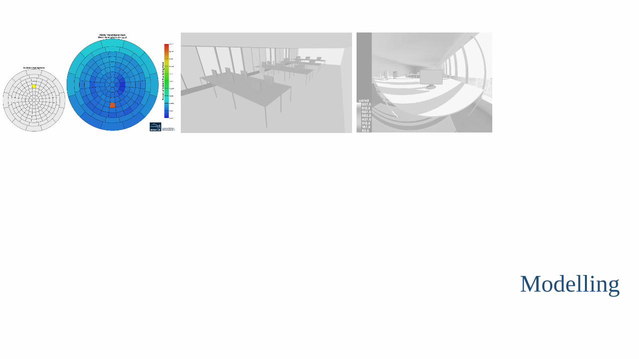
Modelling

Bi-directional Scattering Distribution FunctionModel and material definition
T1
T2
50 x 70
Front
Back
Front
Back
void trans T2 Front & Back
0
0
7 0.7 0.7 0.7 0.01 0 0.56 0
void plastic T1_Front & Back
0
0
5 0.85 0.85 0.85 0 0.05
void plastic T1_Wires
0
0
5 0.85 0.85 0.85 0 0.05
Model dimension 50 x 70 cm
Model dimension 50 x 70 cm

Bi-directional Scattering Distribution FunctiongenBSDF settings
V
T1 T2
V
genBSDF -n 4 -c 4000 -dim 0.280 0.319 0.339 0.396 -0.018 0 +f +b -r '-ab 8' T1 & T2.rad > T1 & T2_bsdf.xml
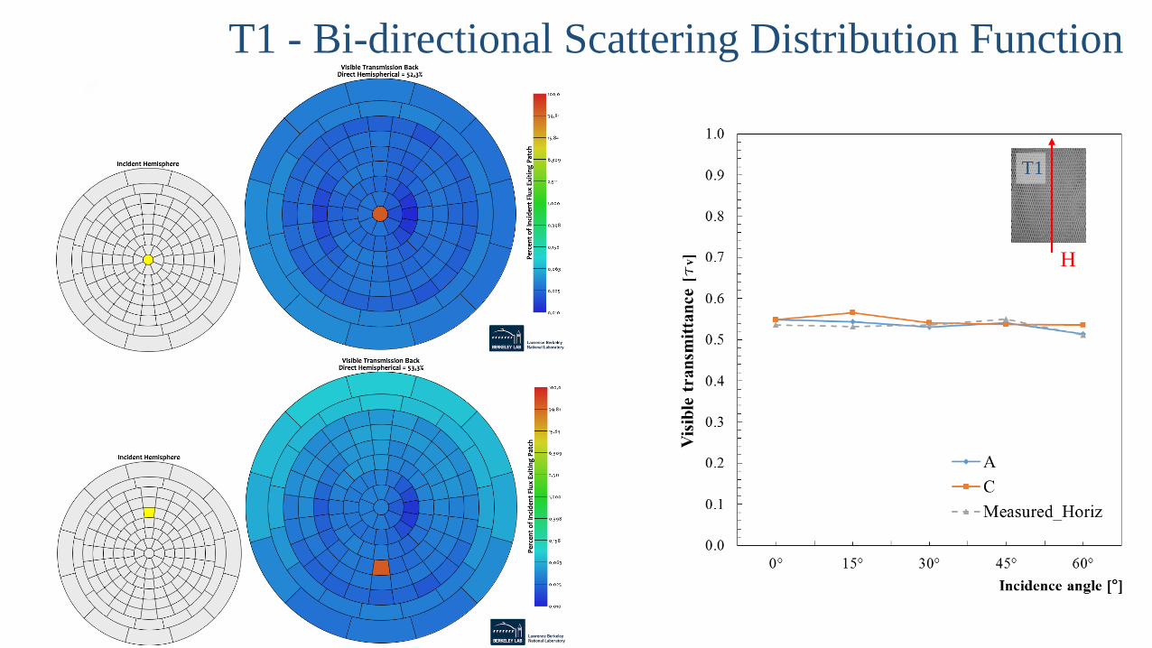
T1 - Bi-directional Scattering Distribution Function
H
T1

T1 - Bi-directional Scattering Distribution Function
V
T1

T2 - Bi-directional Scattering Distribution Function
T2
H

T2 - Bi-directional Scattering Distribution Function
T2
V

A new custom-made 3D textile
void trans TM
0
0
7 0.7 0.7 0.7 0 0 0.47 0

A new custom-made 3D textile

Simulations

ModelGlass - No Shade void glass glazing
0
0
3
0.71 0.71 0.71
Traditional Roller shade void trans Roller_shade
0
0
7
0.87 0.87 0.87 0.000 0.000 0.25 0.05
T2 - 3D Textile roller shade void BSDF Roller_shade
6 0 Shade/T2_bsdf.xml 0 0 1
0
0
TM - 3D Textile roller shade void BSDF Roller_shade
6 0 Shade/TM_bsdf.xml 0 0 1
0
0
Case studies

Model
Wall 0.5
Floor 0.2
Ceiling 0.8
Furniture 0.5
Frame 0.5
Ground 0.3
Glass 0.65
Materials
View position -vp 5.7 1.8 -vd 1 0 0 -vu 0 0 1
-vp 8 1.8 -vd -1 0 0 -vu 0 0 1
Sensor points 0 n0.45 0.8 0 0 1 (680 points)
8 m
12 m
18 m
18 m
2.5 m3
Reflectance Tvis
N

Performances evaluation
Annual simulation - DA, UDI, sDA
• rfluxmtx through Daylight Coefficient Method
Control strategies
• Illuminance level
• Sun penetration depth
Point-in-time simulation - DGP
• rpict through rad
Roller shade
T2
TM

oconv -f material.rad office.rad > temp/office.oct
rfluxmtx -n 4 -I+ -ab 10 -ad 50000 -lw 1e-5 <\
data/points.pts -o matrices/dc_office.mtx -y 680 -\
temp/sky_glow_r4.rad -i temp/office.oct
gendaymtx -m 4 temp/ITA_Milano.wea >\
matrices/Milano.mtx
dctimestep matrices/dc_office.mtx\
matrices/Milano.mtx | rmtxop -fa -c 47.4 119.9 11.6 –t\
- > data/office.ill
$ sh DCmethod.sh
Performances evaluationAnnual Simulation – DC method
DC-method procedure
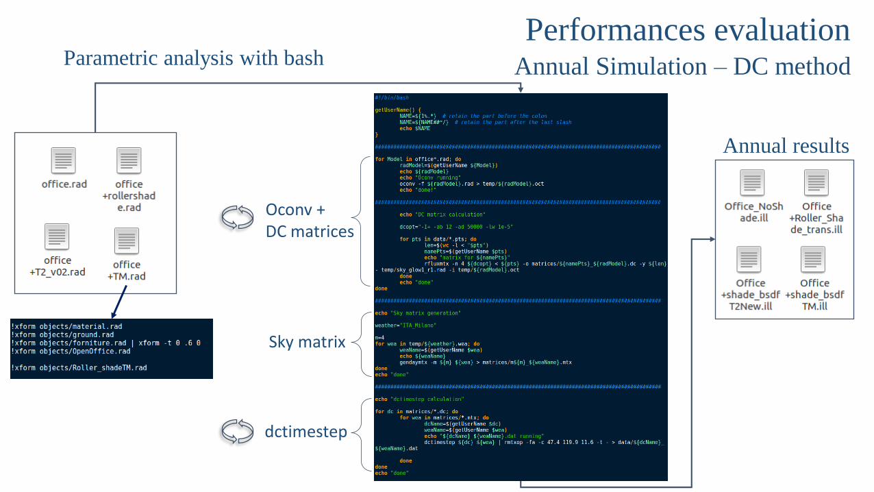
Performances evaluationAnnual Simulation – DC methodParametric analysis with bash
Oconv +DC matrices
dctimestep
Sky matrix
Annual results

Performances evaluationShading control strategies
Horizontal illuminance
• Requires a first run of simulation
• Extract a sensor from the annual simulation
with glass – 1.8 m away from the façade
• Shade is active if Eh > 3000 lux

Performances evaluationShading control strategies
Sun Penetration Depth
• Based on sun angles analysis
• 1st condition: shade is active if the sun reaches
the table - sun penetration > 0.9 m
• 2nd condition: Match statement 1 with the
weather file - ratio total/diffuse hor. irr. > 1.5
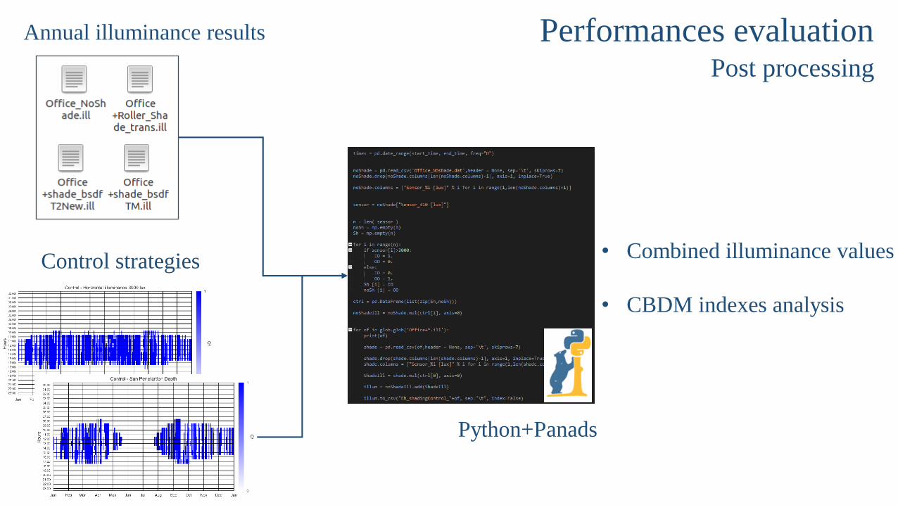
Annual illuminance results
• Combined illuminance values
• CBDM indexes analysis
Performances evaluationPost processing
Control strategies
Python+Panads
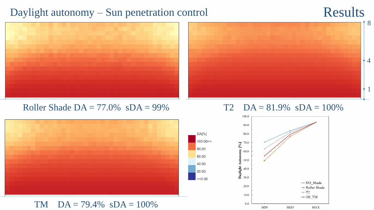
Results
Roller Shade DA = 77.0% sDA = 99% T2 DA = 81.9% sDA = 100%
TM DA = 79.4% sDA = 100%
Daylight autonomy – Sun penetration control
1
4
8

Results300<UDI<3000 – Sun penetration control
Roller Shade UDI = 68.5% T2 UDI = 68.7%
TM UDI = 68.6%
1
4
8

ResultsUDI>3000 – Sun penetration control
Roller Shade UDI = 8.5% T2 UDI = 13.3%
TM UDI = 10.8%
1
4
8
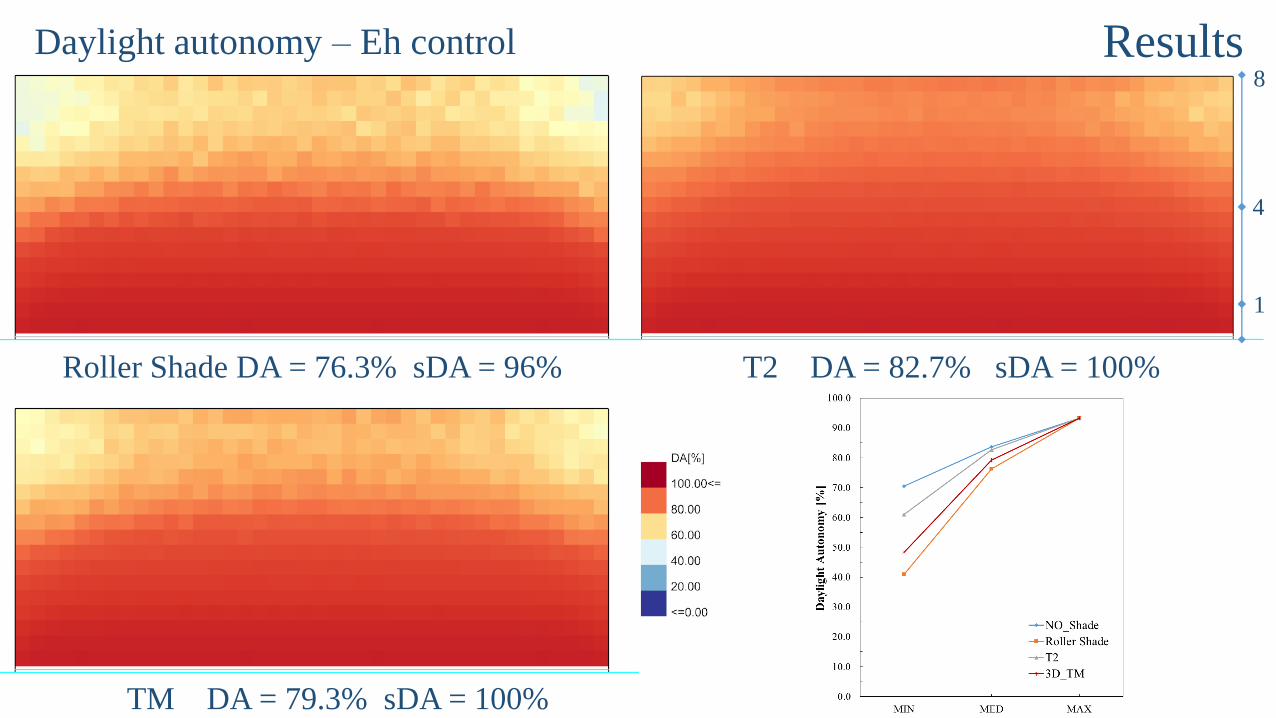
Results
Roller Shade DA = 76.3% sDA = 96% T2 DA = 82.7% sDA = 100%
TM DA = 79.3% sDA = 100%
Daylight autonomy – Eh control
1
4
8
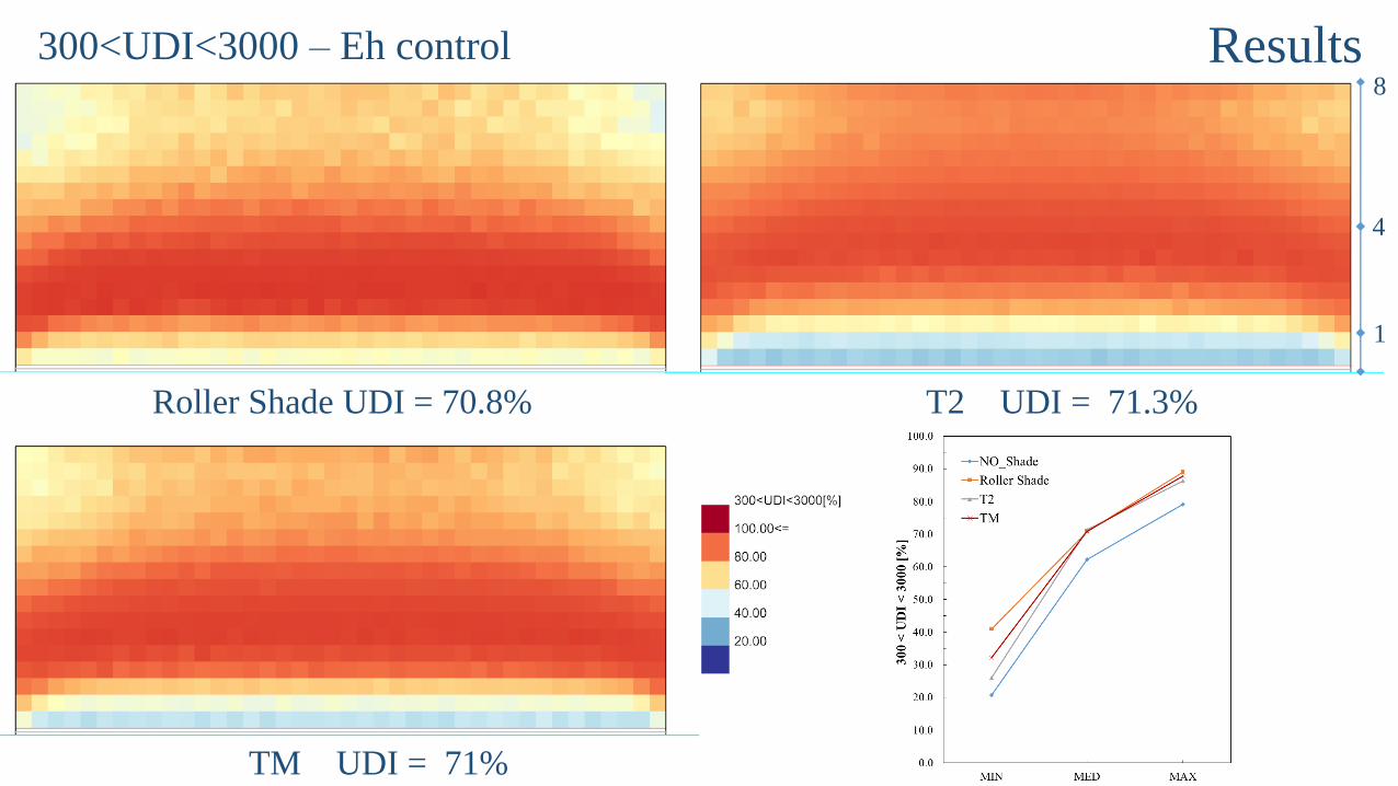
Results300<UDI<3000 – Eh control
Roller Shade UDI = 70.8% T2 UDI = 71.3%
TM UDI = 71%
1
4
8

ResultsUDI>3000 – Eh control
Roller Shade UDI = 5.6% T2 UDI = 11.3%
TM UDI = 8.4%
1
4
8

ResultsSummary
NO STRATEGY CONTROLDA 300 UDI<100 100<UDI<300 300<UDI<3000 UDI>3000 sDA300
NO_Shade 83.74 8.56 7.70 62.24 21.50 100%Roller Shade 50.06 26.17 23.77 47.50 2.56 44%
T2 63.55 18.99 17.46 55.11 8.44 78%3D_TM 55.89 22.97 21.14 50.48 5.42 54%
STRATEGY CONTROL Sun PenetrationDA 300 UDI<100 100<UDI<300 300<UDI<3000 UDI>3000 sDA300
NO_Shade 83.74 8.56 7.70 62.24 21.50 100%
Roller Shade 77.01 9.04 13.95 68.51 8.50 99%
T2 81.98 8.58 9.44 68.67 13.31 100%
3D_TM 79.39 8.76 11.84 68.58 10.82 100%
STRATEGY CONTROL EhDA 300 UDI<100 100<UDI<300 300<UDI<3000 UDI>3000 sDA300
NO_Shade 83.74 8.56 7.70 62.24 21.50 100%Roller Shade 76.36 8.56 15.08 70.79 5.57 96%
T2 82.67 8.55 8.78 71.32 11.35 100%3D_TM 79.31 8.55 12.14 70.92 8.39 100%

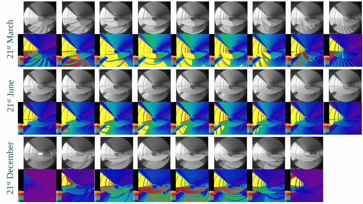
Performances evaluationpoint-in-time simulation – rpict/rad
• Analysis over the standard days
• 21st of March, June and
December
• 9:00-17:00 hours
• Perez sky + epw data
• Creation of the input*.rif file
Procedure to generate the sky file for the
selected days
1. Extend the period of analysis
14-30th March 9:00-17:00
14-30th June 9:00-17:00
14-30th December 9:00-17:00
2. Filter the clear hours on the epw
3. Average values of Direct Normal and
Diffuse Horizontal Irr. -> gendaylit $M $D
$h –W DN DH

Performances evaluationpoint-in-time simulation – rpict/rad
• Creation of the input*.rif file
Write and save the input *.riffile
Run it with rad
Select model and sky
Parametric analysis with bash
radHDR.sh

Performances evaluationpoint-in-time simulation – rpict/rad
26 skies Office no shade
radHDR.sh
evalglare
Glare casesNo glare cases
Office+rollerShade
radHDR.sh
evalglare
Office+T2
Office+TM
“Glare”
skies
DGP>0.4
1st run 2nd run
Combined
glare analysis
21
stM
arch
21
stJu
ne
21
stD
ecem
ber

Results
DGP

21
stM
arch
15:0
0
Roller Shade T2 TM
DGP =0.25 DGP =0.39 DGP =0.30

Conclusion and improvements
• Good fitting between measurements and model
• Improvement in annual daylight performance
• Good control of glare source over the year
• Optimized custom-made 3D textile can guarantee high performance

Conclusion and improvements
• Good fitting between measurements and model
• Improvement in annual daylight performance
• Good control of glare source over the year
• Optimized custom-made 3D textile can guarantee high performance
• Measured BSDF with photogoniometer
• Simulate the fabric surface with BRTDfunc
• Annual glare analysis
• 5-phase method with incorporated geometry

Andrea Zani Giuseppe De Michele [email protected] [email protected]
Thank you for your attention
… any questions?
16th International Radiance Workshop
Portland, Oregon