dayu: fast and low-interference data recovery in very-large … · dayu: fast and low-interference...

This paper is included in the Proceedings of the 2019 USENIX Annual Technical Conference.

July 10–12, 2019 • Renton, WA, USA

ISBN 978-1-939133-03-8

Open access to the Proceedings of the 2019 USENIX Annual Technical Conference

is sponsored by USENIX.

Dayu: Fast and Low-interference Data Recovery in Very-large Storage Systems

Zhufan Wang and Guangyan Zhang, Tsinghua University; Yang Wang, The Ohio State University; Qinglin Yang, Tsinghua University;

Jiaji Zhu, Alibaba Cloud

https://www.usenix.org/conference/atc19/presentation/wang-zhufan

Dayu: Fast and Low-interference Data Recovery in Very-large Storage Systems

Zhufan Wang†, Guangyan Zhang†∗, Yang Wang‡, Qinglin Yang†, Jiaji Zhu§

†Tsinghua University, ‡The Ohio State University, §Alibaba Cloud

AbstractThis paper tries to accelerate data recovery in a large-scalestorage system with minimal interference to foreground traffic.By investigating I/O and failure traces from a real-world large-scale storage system, we find that because of the scale of thesystem and the imbalanced and dynamic foreground traffic,no existing recovery protocols can generate a high-qualityrecovery strategy in a short time.

To address this problem, this paper proposes Dayu, atimeslot-based recovery protocol, which only schedules a sub-set of tasks which are expected to finish in one timeslot: thisapproach reduces the computation overhead and naturally cancope with the dynamic foreground traffic. In each timeslot,Dayu incorporates four key algorithms, which enhance exist-ing solutions with heuristics motivated by our trace analysis.

Our evaluations in a 1,000-node real cluster and in a 25,000-node simulation both confirm that Dayu can outperform exist-ing recovery protocols, achieving high speed and high quality.

1 Introduction

This paper describes our experience and methods to acceleratedata recovery in Pangu [1] , a real-world large-scale storagesystem with 10K nodes and tens of TBs of storage per node.

As a cloud storage provider, AliCloud, the owner of Pangu,needs to make a promise of data durability to its customers(i.e., the chance of data loss is smaller than a threshold). Formarketing reasons, the owner has a strong motivation to im-prove data durability, so that its promise can be appealingcompared to its competitors. This motivates us to investigatewhether it is possible to accelerate data recovery in Pangu,because recovery speed is one of the determining factors ofdata durability [2].

Similar to previous works [3–7], Pangu divides data intochunks (usually tens of MBs), replicates these data chunks,and distributes these replicas to different nodes. When a nodefails, Pangu re-replicates its data chunks: since the replicas of∗Corresponding author: [email protected]

these chunks are distributed to different nodes, Pangu asks allthese nodes to copy chunks in parallel [4, 8].

To re-replicate data chunks of the failed node, the recov-ery protocol needs to schedule a source, a destination, and abandwidth for each of these data chunks. An ideal schedulingalgorithm should achieve at least the following two goals: first,the algorithm should generate a high-quality strategy, whichshould allow data re-replication to be completed as soon aspossible under the constraint that it has minimal impact onforeground traffic; second, the speed of the scheduling algo-rithm itself should be high enough so that it does not becomethe bottleneck of data recovery.

To understand the quality and speed of existing schedulingalgorithms, we analyze the failure and I/O traces from a realdeployment of Pangu. We find none of the existing algorithmscan achieve both acceptable quality and acceptable speed,because of the following challenges:

• Very-large scale: the largest deployment of Pangu hasmore than 10K nodes and up to 72 TBs of storage (about1.5M chunks) per node. Therefore, when a node fails,the algorithm needs to decide how to recover all thesedata chunks and each chunk has about 10K nodes ascandidate destinations.

• Tight time constraint: given the scale of the system, datachunks of a failed node can be re-replicated with a highdegree of parallelism. Our simulation shows that if theidle bandwidth can be fully utilized, the recovery can befinished within tens of seconds, which means the schedul-ing algorithm itself should complete within seconds.

• Imbalanced foreground traffic and available data: wefind a two-fold imbalance, which poses challenges to thequality of scheduling. First, a number of nodes can havesignificantly heavier foreground traffic than the others;and second, some nodes can have more data chunksavailable for re-replication.

• Dynamic foreground traffic: the foreground traffic canchange dramatically over time. To cope with such dy-namic traffic, the recovery protocol needs to adjust its

USENIX Association 2019 USENIX Annual Technical Conference 993

plan when it observes a significant change in the fore-ground traffic, which again calls for fast scheduling.

Our simulation of existing scheduling algorithms showsthat, on the one hand, simple and decentralized algorithmslike random selection or best-of-two-random [9] can finishscheduling quickly (i.e., high speed), but they often cause asmall number of nodes to be overloaded, increasing the recov-ery time and impairing the performance of foreground traffic(i.e., low quality). On the other hand, sophisticated and cen-tralized algorithms, such as Mixed-Integer Linear Program-ming [10–12], can effectively utilize available bandwidth andavoid overloading a node (i.e., high quality), but they can takeprohibitively long to compute a plan given the scale of ourtarget system (i.e., low speed).

This paper proposes Dayu, a high-speed and high-qualityrecovery protocol for large-scale, imbalanced, and dynamicstorage systems. The key idea of Dayu is motivated by theobservation that, to cope with dynamic foreground traffic,we need to periodically monitor the foreground traffic andadjust the recovery plan: in such a design, scheduling forall data chunks of the failed node together is both computa-tionally heavy and unnecessary, since the plan is likely to beadjusted later. Following this observation, Dayu incorporatesa timeslot-based solution: it divides time into multiple slots,whose length is determined by how frequent the underlyingstorage system monitors and reports idle bandwidth; basedon such report, Dayu tries to schedule a subset of chunks sothat they can be re-replicated within the current timeslot; ifthe actual re-replication of some chunks takes longer thanexpected for whatever reason, Dayu will re-schedule them inthe next timeslot.

This approach brings two benefits: first, it reduces the com-putation overhead of scheduling because in each timeslot, thealgorithm only needs to schedule a subset of tasks (about onethird on average in our experiments). Second, this solutioncan naturally cope with the dynamic foreground traffic be-cause Dayu’s decision is based on the information collectedat the beginning of each timeslot.

To realize this idea, Dayu incorporates four key techniques,which enhance existing algorithms based on our observations:

• Greedy algorithm with bucket convex-hull optimizationto schedule tasks: Dayu uses a greedy algorithm to it-eratively choose the most under-utilized candidate asthe source and destination for each task, till it findsenough tasks to fill a timeslot. To reduce the computationoverhead, Dayu incorporates the convex-hull optimiza-tion [13] and further proposes a bucket approximationto reduce the size of the candidate set.• Prioritizing nodes with high idle bandwidth but few avail-

able chunks: Our observation shows that such nodesare likely to get under-utilized, if the scheduling algo-rithm decides to replicate their chunks from other nodes.Therefore, Dayu enhances the aforementioned greedy

algorithm with the following heuristic: if a chunk to bere-replicated has a replica in such a prioritized node,Dayu will assign the node as the source.• Iterative WSS to allocate bandwidth for each task: To

minimize the completion time of chosen tasks, Dayuenhances the weighted shuffle scheduling algorithm(WSS) [14]: in each iteration, Dayu uses WSS to iden-tify the bottlenecks in the remaining tasks, assigns aweighted fair share of bandwidth to each task correspond-ingly, and removes the bottleneck tasks and allocatedbandwidth.• Re-scheduling stragglers: Straggler tasks will inevitably

occur due to mis-prediction of the foreground traffic orunexpected hardware faults, so Dayu has to re-schedulethem in the next timeslot. Straggler tasks are differentfrom new tasks, since we prefer keeping their destina-tions unchanged: otherwise, we will lose their existingprogress. Dayu first estimates whether it is worth chang-ing their destinations, and then re-computes their sourcesand allocated bandwidth.

Our evaluation of Dayu on a real deployment of 1,000nodes shows that, compared to Pangu, Dayu increases therecovery speed by 2.96× and increases the p90 latency (i.e.,tail latency at 90th percentile) of the foreground traffic duringrecovery by only 3.7%. Our simulation shows that Dayu out-performs various existing solutions and can scale to a clusterof 25K nodes.

2 Background and Observations

2.1 Background of PanguPangu is the underlying storage system of AliCloud, one ofthe largest public cloud providers in Asia [1]. Pangu inheritsthe classic distributed file system architecture from previousworks like GFS [3], HDFS [5], Cosmos [6], and Azure [7].It splits data into multiple chunks (the most common chunksize is 64MB) and stores data chunks on a large number ofdata servers called ChunkServers. A metadata server calledMetaServer maintains the metadata of the distributed file sys-tem, such as the locations of data chunks. Given its verylarge scale, Pangu incorporates multiple MetaServers, eachresponsible for a subset of metadata [15–17]. Besides, Panguincorporates a RootServer to route clients to the correspond-ing MetaServer. To achieve uniform data distribution, Panguuses random or weighted random mechanism to place data ondifferent ChunkServers.

Like most existing systems, Pangu replicates data chunks(most chunks have three replicas) so that if a node fails, Pangucan recover its data chunks by copying from other replicas.For each data chunk to be recovered, Pangu needs to choose asource and a destination for data copy: there are usually a fewcandidate sources depending on the number of replicas and a

994 2019 USENIX Annual Technical Conference USENIX Association

large number of candidate destinations. The current versionof Pangu randomly picks a source and a destination for eachdata chunk to be recovered.

In the current deployment of Pangu, we observe that thenetwork bandwidth is usually the bottleneck when performingsuch data recovery: most Pangu nodes are equipped with 1Gbor 10Gb Ethernet, whose bandwidth is smaller than the aggre-gate disk bandwidth; the deployment of high-speed devices,such as Infiniband, is limited due to cost reasons. Pangu’score network switches are organized using CLOS topologyor fat-tree topology [18–21], so that there is no oversubscrip-tion. The core-to-rack link may be oversubscribed dependingon the configuration: if the link is oversubscribed, the rackswitch is usually the bottleneck; if not, the NICs of end-hostsare the bottlenecks.

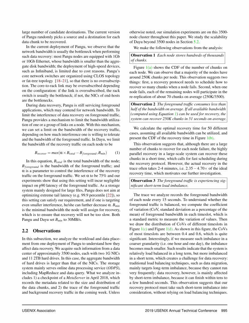
During data recovery, Pangu is still servicing foregroundapplications, which may contend for network bandwidth. Tolimit the interference of data recovery on foreground traffic,Pangu provides a mechanism to limit the bandwidth utiliza-tion of one or a group of links on a node. With this mechanism,we can set a limit on the bandwidth of the recovery traffic,depending on how much interference one is willing to tolerateand the bandwidth of the foreground traffic. In Dayu, we limitthe bandwidth of the recovery traffic on each node to be

Brecover = max(α×Btotal−B f oreground ,Bmin) (1)

In this equation, Btotal is the total bandwidth of the node;B f oreground is the bandwidth of the foreground traffic; andα is a parameter to control the interference of the recoverytraffic on the foreground traffic. We set α to be 75% and ourexperiments show that using this setting will incur negligibleimpact on p90 latency of the foreground traffic. As a storagesystem mainly designed for large files, Pangu does not aim atoptimizing extreme tail latency (e.g. 99.9 percentile [22]), sothis setting can satisfy our requirement, and if one is targetingeven smaller interference, he/she can further decrease α. Bminis the minimal bandwidth the node will assign for recovery,which is to ensure that recovery will not be too slow. BothPangu and Dayu set Bmin to 30MB/s.

2.2 ObservationsIn this subsection, we analyze the workload and data place-ment from one deployment of Pangu to understand how theyaffect data recovery. We acquire such information from a datacenter of approximately 3500 nodes, each with two 1G NICsand 11 2TB hard drives. In this case, the aggregate bandwidthof hard drives is larger than that of the NICs. The storagesystem mainly serves online data processing service (ODPS),including MapReduce and data query. What we analyze in-cludes 1) a checkpoint of a MetaServer in April 2018, whichrecords the metadata related to the size and distribution ofthe data chunks, and 2) the trace of the foreground trafficand background recovery traffic in the coming week. Unless

otherwise noted, our simulation experiments are on this 3500-node cluster throughout this paper. We study the scalabilityof Dayu beyond 3500 nodes in Section 5.2.

We make the following observations from the analysis:

Observation 1 Each node stores hundreds of thousandsof chunks.

Figure 1(a) shows the CDF of the number of chunks oneach node. We can observe that a majority of the nodes havearound 250K chunks per node. This observation suggests twothings: first, a recovery protocol needs to schedule how torecover so many chunks when a node fails. Second, when onenode fails, each of the remaining nodes will participate in there-replication of about 70 chunks on average (250K/3500).

Observation 2 The foreground traffic consumes less thanhalf of the bandwidth on average. If all available bandwidth(computed using Equation 1) can be used for recovery, thesystem can recover 250K chunks in 51 seconds on average.

We calculate the optimal recovery time for 50 differentcases, assuming all available bandwidth can be utilized, andpresent the CDF of the recovery time in Figure 1(b).

This observation suggests that, although there are a largenumber of chunks to recover for each node failure, the highlyparallel recovery in a large-scale system can recover thesechunks in a short time, which calls for fast scheduling duringthe recovery protocol. However, the actual recovery in thetrace often takes 2-4 minutes, i.e. 2.35−4.70× of the idealrecovery time, which motivates our further investigation.

Observation 3 The foreground traffic is experiencing sig-nificant short-term load imbalance.

The trace we analyze records the foreground bandwidthof each node every 15 seconds. To understand whether theforeground traffic is balanced, we compute the coefficientof variation (CoV, standard deviation as a percentage of themean) of foreground bandwidth in each timeslot, which isa standard metric to measure the variation of values. Thenwe draw the distribution of CoVs of different timeslots inFigure 1(c) and Figure 1(d). As shown in this figure, the CoVsof most timeslots are between 0.4 and 0.6, which is quitesignificant. Interestingly, if we measure such imbalance in acoarser granularity (i.e. one hour and one day), the imbalancebecomes much smaller. Such results indicate that the system isrelatively load balanced in a long term, but more imbalancedin a short term, which creates a challenge for data recovery:traditional load balancing techniques, such as data migration,mainly targets long-term imbalance, because they cannot runvery frequently; data recovery, however, is mainly affectedby short-term imbalance, because it can finish within tens toa few hundred seconds. This observation suggests that ourrecovery protocol must take such short-term imbalance intoconsideration, without relying on load balancing techniques.


250K 500K 750K

Number of chunks

0.0

0.2

0.4

0.6

0.8

1.0

Cum

ulat

ive

frac

tion

(a) OB1: CDF of the number ofchunks on each node

0 25 50 75 100

Recovery time (s)

0.0

0.2

0.4

0.6

0.8

1.0

Cum

ulat

ive

frac

tion

(b) OB2: CDF of the optimal recov-ery time with 50 cases

0.2 0.4 0.6 0.8CoV of foreground traffic

0.0

0.2

0.4

0.6

0.8

1.0

Cum

ulat

ive

frac

tion

15 secs.

1 hour

1 day

(c) OB3: CoV of outgoing band-width utilization

0.2 0.4 0.6 0.8CoV of foreground traffic

0.0

0.2

0.4

0.6

0.8

1.0

Cum

ulat

ive

frac

tion

15 secs.

1 hour

1 day

(d) OB3: COV of incoming band-width utilization

20 40 60 80

Size of common chunks (GB)

0

150

300

450

Num

ber

ofno

des

(e) OB4: Distribution of SC100j .

0.2 0.4 0.6 0.8

CoV of common chunk size

0.0

0.2

0.4

0.6

0.8

1.0

Cum

ulat

ive

frac

tion

(f) OB4: CoV of SCij for each node i

0 25 50 75 100

Common chunk size (GB)

0

10

20

30

40

Tra

nsm

issi

onsi

ze(G

B)

(g) OB4: Correlation between recov-ery traffic of node j and SC100

j

−100 0 100

Delta bandwidth(MB/s)

0.0

0.2

0.4

0.6

0.8

1.0

Cum

ulat

ive

frac

tion

p97.5 = 34

p2.5 = -36

(h) OB5: Bandwidth utilization vari-ance.

Figure 1: Observations from a 3500-node real-world system

Observation 4 Replicas of chunks on a given nodes aredistributed unevenly among the other nodes.

To understand how replicas of chunks on a given node aredistributed among the other nodes, we define SCi

j as the sizeof the chunks held by both node i and node j, which showshow much data node j can provide as source during recoveryif node i fails.

We first sample a specific node i = 100. Figure 1(e) showsthe distribution of SC100

j for different j values. We can see thatthe histogram of the distribution fits the bell curve: this is ac-tually mathematically provable (i.e. Central Limit Theorems)if we assume chunk placement is random. To understand suchimbalance in the whole cluster, for each node i, we calculatethe CoV of all the SCi

j values and then we draw the CDF ofCoVs of all nodes in Figure 1(f). One can observe that for alarge portion of nodes, the distribution of SCi

j is not balanced.To understand how such imbalance affects recovery, we

simulate the failure of node 100 with Pangu’s random nodeselection strategy (Figure 1(g)) and find that there is a strongcorrelation between the size of outgoing recovery traffic ofnode j and SC100

j . That means a node with a few (many) com-mon chunks with the failed node will do little (much) workduring recovery, but if the node has much (little) availablebandwidth, it will get under-utilized (overloaded).

Observation 5 Foreground traffic usually fluctuates within14.4% of max bandwidth, but sometimes can change dra-matically.

Figure 1(h) shows how one node’s foreground trafficchanges in 5 hours. The delta bandwidth is the difference

of the average bandwidth utilization in two adjacent timeslots.We can observe that in more than 95% of the cases (between“p2.5” and “p97.5” in Figure 1(h)), the absolute delta band-width is lower than 36MB/s, which is 14.4% of the maximumbandwidth (250 MB/s since each node has two 1Gb NICs).However, in the remaining 5% cases, the delta bandwidth canreach up to two thirds of the maximum bandwidth. Althoughthe percentage of such extreme cases is small, they frequentlyhappen in recovery, because the highly parallel recovery usu-ally involves many nodes. Our simulation shows that they cancreate stragglers in recovery and thus are one of the majorreasons why recovery speed is not ideal.

3 Dayu Overview

We call the re-replication of one data chunk a “recovery task”in the rest of the paper. Dayu achieves fast data recoveryand low application interference by introducing a centralizedscheduler called an ObServer, which performs timeslot-basedrecovery task scheduling.

Dayu assumes all the data servers periodically report theirchunk placement and network utilization to the ObServer,and all the metadata servers send information of the recoverytasks to the ObServer. The rest of this paper presents theObServer’s scheduling algorithm, which decides the source,the destination, and the bandwidth of a recovery task.

To achieve high-speed and high-quality scheduling, thekey idea of Dayu is to schedule recovery tasks in multiplebatches, instead of scheduling all of them together. This de-sign choice is motivated by several reasons: first, since eachnode is usually involved in tens of recovery tasks (Observa-


Replication begin Replication finish

Time

Gathering

Scheduling

TransmittingTimeslot 0

Timeslot 1

Timeslot 2

Figure 2: Timeslot-based scheduling in Dayu

Ttimeslot Length of a timeslotBi

recover_in/out Node i’s available incoming/outgoingbandwidth for recovery (by Equation 1)

st Size of recovery task tci

in/out Total size of incoming/outgoing recov-ery tasks assigned to node i

α, β Parameters

Table 1: Denotations

tion 1), scheduling tasks in multiple batches can still alloweach node to fully participate in each batch and thus fullyutilize its available bandwidth; second, scheduling tasks inbatches can naturally cope with dynamic foreground trafficand infrequent measurement errors, because when observingany changes in the foreground traffic, Dayu can make adjust-ment in the next batch; finally, scheduling tasks in batchesnaturally reduces the computation overhead of the schedulingalgorithm, because for each batch, the algorithm only needsto schedule a subset of tasks.

To implement this idea, as shown in Figure 2, Dayu di-vides the whole recovery time into multiple fixed-length timeslices (called timeslots throughout the paper). At the begin-ning of a timeslot, the ObServer collects the latest state of thedata servers. Using the state obtained, the ObServer choosesand schedules a subset of recovery tasks in this timeslot, in-cluding those recovery tasks scheduled in the last timeslot butunfinished yet. To fully utilize the available bandwidth, Dayuoverlaps multiple timeslots so that the information gatheringand task scheduling of slot n is executed before the end ofslot n− 1. The length of a timeslot is determined by howfrequently the underlying storage system collects and reportsstate.

As mentioned in Section 2.1, the bottleneck of data recov-ery is either the NICs of the end hosts or the rack switch, andto simplify description, the following text assumes the NICsof the end hosts are bottlenecks, and one can easily extend it tosupport bottleneck rack switches. Table 1 lists the denotationsused in the paper.

Goals. Dayu tries to achieve the following goals.

• Goal 1: Utilize the available bandwidth as much aspossible. This is a natural goal to minimize the overallrecovery time. If we were to fully utilize the available

bandwidth in one timeslot, the total size (S) of the chunksthat can be replicated in the timeslot would be:

S = min( ∑i∈Nodes

Birecover_in, ∑

i∈NodesBi

recover_out)×Ttimeslot (2)

• Goal 2: Finish as many tasks as possible in the targettimeslot. We hope that the scheduled tasks can actuallyfinish within the target timeslot: otherwise, we have tore-schedule them again, which increases the computa-tion overhead. This goal may look similar to the first one,but it is not: the first goal suggests us to oversubscribethe network bandwidth (i.e. schedule more tasks than thebandwidth can handle), so that if the foreground trafficdrops, we can still utilize such extra available bandwidth;the second goal, however, suggests us to undersubscribethe network bandwidth so that if the foreground trafficincreases, we can still finish the scheduled tasks. There-fore, Dayu has to make a trade-off between these twogoals.• Goal 3: Minimize the chance of significant stragglers.

Because we cannot accurately predict the future fore-ground traffic, stragglers will inevitably occur. We prefermany small stragglers to a few significant stragglers, be-cause many small stragglers can be re-scheduled andexecuted in parallel to minimize the recovery time. How-ever, this goal obviously contradicts with the second goal,so Dayu has to make a trade-off as well.

Overview of Dayu’s algorithm. To achieve these goals,Dayu incorporates four key techniques, by enhancing existingalgorithms with heuristics and approximations motivated byour observations: 1) a greedy algorithm with bucket convexhull optimization to select the source and the destination foreach recovery task (§4.1); 2) a heuristic-based algorithm toprioritize nodes with a few common chunks with the failednode but a high available bandwidth (§4.2); 3) an iterativeWSS algorithm to assign bandwidth for each task (§4.3);and 4) a heuristic-based algorithm to minimize the cost ofre-scheduling straggler tasks (§4.4).

4 Design of Dayu

4.1 Selecting Source and DestinationDayu iteratively scans all tasks and determines the source andthe destination for each task, till it can find enough tasks tofill S (Equation 2). The candidate sources of a task include allnodes which hold a replica of the corresponding chunk; thecandidate destinations of a task include all nodes which arenot in the same rack of its sources.

To achieve the goals given in Section 3, Dayu incorporatesa greedy algorithm: for each task, Dayu chooses the mostunder-utilized node in its candidate sources and destinations;


(Bi,c

i)

(0,-st)Available bandwidth

Accu

mula

ted

siz

e

(a) Convex hull optimization

Available bandwidth

Accu

mula

ted

siz

e(b) Bucket approximation

Figure 3: Reduce computation overhead with dynamic convexhull optimization. Bi and ci are short for Bi

recover_in and ciin.

if Dayu finds that even the most under-utilized candidate isgoing to be saturated, Dayu will skip this task.

The first question we need to answer is how to quantita-tively measure the utilization of a node. We have tried severaloptions, and through simulation, we decide to use the expectedtask finish time

cin/outBrecover_in/out

(cin/out is the total size of the in-coming/outgoing tasks assigned to this node) as the metric toevaluate the utilization of a node, because this metric achievesa nice balance between our first two goals.

Therefore, when choosing the source for task t, Dayu scansall its candidate nodes and chooses the one with the minimal

st+coutBrecover_out

as the source. Such scanning is not computationallyexpensive, since most chunks have three replicas and oneof them is already lost. Afterward, Dayu checks whetherassigning task t to the source will saturate the source, i.e. its

st+coutBrecover_out

> Ttimeslot : if so, Dayu will drop task t, because thismeans there is no way to complete task t in this timeslot.

Likewise, when choosing the destination for task t, Dayuchooses the node with the minimal st+cin

Brecover_in. However, naively

scanning all candidate destinations is computationally heavy,since the number of candidate destinations is large. To makethings worse, greedy algorithms cannot be parallelized be-cause each iteration depends on the result of the previousiteration. Our simulation on a 3500-node cluster shows thatnaively scanning all candidate destinations for each task canonly achieve a speed of less than 30,000 tasks per second.Since our statistics shows that in one timeslot, Dayu canusually complete 60,000—150,000 tasks, this means naivelyscanning itself will take 2-5 seconds, which is not ideal. Toaddress this challenge, we incorporate the dynamic convexhull optimization to accelerate this computation.

One can refer to [13] for the formal description of theconvex hull optimization, and here we present an intuitivedescription. For each surviving node i, we draw a point(Bi

recover_in,ciin) in Cartesian coordinate system, as shown in

Figure 3(a). Then for task t with size st , we draw anotherpoint (0,−st) in Figure 3(a). Afterward, we draw a line from(0,−st) to each other point: since the slope of each line is

ciin+st

Birecover_in

, finding the destination node for task t is equivalent

to finding the line with the lowest slope.

We can maintain a dynamic convex hull to quickly searchthe line with the lowest slope. In a two-dimensional space,a convex hull is like a rubber band that wraps all the pointstightly, where the lower convex shell is the lower part ofthis convex hull. We refer the point set of the lower convexshell as H (here we connect points in H together to formthe lower convex shell as shown in Figure 3(a)). The pointsin H are connected counterclockwise. Then for a point phwith precursor point and successor point in set H, the slope ofline ph−1→ ph must be less than or equal to the slope of lineph→ ph+1. We can find the node c in set H whose connectionwith point (0,−st ) has the smallest slope using binary searchand the time complexity is O(log |H|).

After Dayu assigns task t to node i, its ciin is incremented

by st . Therefore, Dayu needs to adjust the point of node i aswell as the lower convex shell H: when a point ph in H movesup, Dayu identifies the precursor (ph−1) and successor (ph+1)of ph in original H, and scans all the points between them tofind the new member(s) of H. The convex hull optimizationreduces the complexity of scanning destination nodes fromlinear to sub-linear, without affecting the results of the greedyalgorithm.

We further propose an approximate solution to reduce thecandidate set of the lower convex shell, in turn boosting thespeed of the algorithm. As shown in Figure 3(b), we divide therange of available incoming bandwidth into multiple equal-sized buckets. If nodes i and j are in the same bucket, they areconsidered to have approximately identical available band-width, i.e. Bi

recover_in ≈ B jrecover_in. Without loss of generality,

we suppose ci > c j. Then node i cannot be the member of thelower convex shell. Therefore, only the lowest node withinthe same bucket can become the member of the lower convexshell. All those lowest nodes (hollow circles in Figure 3(b))form a reduced candidate set, denoted C. We can constructthe convex shell H from this reduced candidate set C, insteadof the full set of nodes. After Dayu assigns a task to a node, itadjusts the point of this node as well as the reduced candidateset.

The bucket size determines the reduction degree of thebucket approximation. We use 1 MB/s as the bucket size in ourexperiments, and our simulation shows an average reductionfactor of 22.8, and as a result, Dayu can complete selectingsources and destinations for about 210,000 chunks within onesecond—this is seven times faster than naive scanning.

Such bucket approximation certainly brings inaccuracy tothe greedy algorithm, but such inaccuracy already exists asa result of measurement errors and fluctuation of foregroundtraffic. Therefore, as long as the bucket size is small, our ap-proximation should not significantly increase such inaccuracy.


4.2 Prioritizing Underemployed Nodes

Our simulation on our greedy algorithm reveals the sameproblem as our Observations 3 and 4: nodes with high avail-able bandwidth but only a small number of available chunksare likely to get under-utilized, which violates our first goal.We call them underemployed nodes in the rest of the paper.For example, suppose node A has an available outgoing band-width of 50MB/s and can be the source of Tasks 1 and 2; nodeB has an available outgoing bandwidth of 60MB/s and can bethe source of Tasks 1-4; all tasks have the same size. In thisexample, the optimal schedule should let A be the source ofTasks 1 and 2, and B be the source of Tasks 3 and 4. However,if our greedy algorithm scans Task 1 first, it will assign it tonode B, because B has more available bandwidth than A atthis moment.

This observation suggests that, for a chunk which has areplica in an underemployed node, it’s better to use the un-deremployed node as the source. To achieve this goal, weincorporate a distribution-driven prioritizing strategy: the Ob-Server first sorts all the nodes according to their availableoutgoing bandwidth in descending order, and sorts all thenodes according to their total sizes of common chunks inascending order. Then, the ObServer picks the first β (5% inour typical settings) nodes from those two node lists respec-tively to form two sets, and gets the underemployed node setby computing the intersection of those two sets. Next, theObServer selects all the recovery tasks that have replicas inthe underemployed nodes, and puts them in a queue called“prioritized queue”; the ObServer puts the rest of the tasks inanother queue called “normal queue”.

We modify our greedy algorithm (§4.1) to incorporate thisheuristic: the ObServer will first scan tasks in the prioritizedqueue and directly use the corresponding underemployedserver as the source, instead of using the most under-utilizedcandidate. There are two corner cases: 1) it is possible that aprioritized task has replicas in more than one underemployedservers. In this case, the ObServer chooses the most under-utilized one among them; 2) though rare, it is possible that theunderemployed server is saturated. In this case, the ObServerdegrades the prioritized task into the normal queue, so thatlater we can still try its non-prioritized candidates.

Overhead. When searching underemployed nodes, Dayumaintains two heaps, whose keys are the available outgoingbandwidth and the total size of common chunks respectively,and whose values are the IDs of nodes. The ObServer willfirst build these two heaps, which is an O(n) operation (nis the number of nodes) [23], and then pop 5% entries fromthese two heaps, with each pop an O(logn) operation. Ourexperiment shows that heapifying 10,000 entries and thenpopping up 5% of them only take a few miliseconds.

4.3 Allocating Bandwidth for Each Task

Given the source and destination of each recovery task, weneed to answer how fast each task should proceed. A naivesolution is to set a coarse-grained limit on all tasks within onenode using Brecover_in/out and let them compete for bandwidth.However, our experiments have revealed two problems withthis approach: first, this approach may cause a congestionwhen the source’s outgoing limit is larger than the destina-tion’s incoming limit. Although TCP can resolve such con-gestion eventually, it will cause packet drops and slow downrecovery. Second, the competition may cause one task to besignificantly slower than others, causing a significant stragglerand violating our third goal.

Therefore, in this step, Dayu tries to set a constant ratefor each task in one timeslot, with the goal of maximizingbandwidth utilization. Recall that we assume the NICs of theend hosts are the bottlenecks, so this step only considers thebandwidth utilization at the end hosts. Even so, this is still achallenging problem, since allocating bandwidth for a taskwill consume the bandwidth on both sides.

Dayu’s solution is based on weighted shuffle scheduling(WSS) [14], a mature network scheduling algorithm designedfor scheduling large data flows like data shuffle in MapRe-duce [24]. The key idea of WSS is that, to finish all the pair-wise transfers at the same time, it guarantees that 1) transferrates are proportional to data sizes for each transfer, and 2) atleast one link is fully utilized. With WSS, only the bottlenecklinks (quite a minority) are fully used, while all the othershave an amount of bandwidth left. In our scenario, however,WSS is not ideal: when considering unpredictable growth inforeground traffic, which may cause a non-bottleneck link tobecome a bottleneck in the middle of a timeslot, WSS maycause a waste of bandwidth, because Dayu could utilize morebandwidth of this link at the beginning.

To this end, Dayu introduces an iterative WSS solution toallocate bandwidth for each task. Its key idea is that, withoutdelaying the bottleneck tasks, we should finish other tasks asearly as possible, so as to reduce their completion time and toimprove bandwidth utilization. Following this idea, if there isany remaining bandwidth after running one iteration of WSS,Dayu will use another iteration of WSS to identify the nextbottleneck and allocate the remaining bandwidth.

To be specific, Dayu maintains a remaining incoming andoutgoing bandwidth Bi

remain_in and Biremain_out for each node,

whose initial values are Birecover_in and Bi

recover_out . In each

iteration, Dayu first finds the node with the longest ciin

Biremain_in

or ciout

Biremain_out

, denoted T ∗: the corresponding tasks are the bot-

tlenecks. Then, Dayu allocates Bt =stT ∗ bandwidth to each

task t, indicating that to minimize the completion time, thebottleneck tasks must be assigned a weighted fair share of thebandwidth, such that the weight of the share is proportionalto st . Afterward, Dayu updates the remaining bandwidth as


Biremain_in−=

ciin

T ∗ and Biremain_out−= ci

outT ∗ for each node i, re-

moves the bottleneck tasks from their corresponding nodes,and updates the cin/out values of these nodes. Then Dayumoves to the next iteration with the remaining tasks, till thereare no tasks remaining or the remaining tasks have an accept-able transmission time (i.e., less than or equal to the lengthof a timeslot) with their allocated bandwidth. Note that if atask goes through multiple iterations, its allocated bandwidthis the sum of the allocated bandwidth in each iteration.

Iterative WSS overcomes the drawbacks of WSS: sinceiterative WSS tries to allocate all bandwidth, it is not possiblefor the system to waste bandwidth when there are tasks thatcan utilize such bandwidth.

Our experiment shows that for a 3500-node cluster, eachiteration will take at most 15 ms. Since dynamic convex hullnode selection algorithm keeps the “ c

B " values of most nodesto be close, the iterative WSS algorithm can usually finishwithin five iterations (i.e. 75 ms), which is acceptable.

4.4 Re-scheduling Straggling TasksDue to inaccurate workload estimation, sub-optimal schedul-ing, hardware exceptions, and etc., some tasks could not befinished at the end of one timeslot. Dayu has to re-schedulesuch straggler tasks in the next timeslot, but cannot simplytreat them as new tasks, because changing the destinationof one straggler task requires re-transmitting the task fromthe beginning, causing waste of bandwidth. Therefore, Dayushould avoid changing the destination when possible—this isa constraint new tasks do not have.

Identifying stragglers. Recall that Dayu overlaps differenttimeslots so that the scheduling phase of the current timeslothappens a short period of time (denoted as Tschedule) beforethe end of the last timeslot (Figure 2). Therefore, Dayu has topredict which tasks will become stragglers: for one unfinishedtask, Dayu uses its speed so far to estimate its speed till theend of the last timeslot; if the task cannot finish given theestimated speed, Dayu puts those tasks into a straggler set.

Prediction can certainly be inaccurate. If Dayu marks a taskas a straggler but it actually finishes with the last timeslot, thecorresponding nodes will simply ignore the new transmissionplan scheduled by Dayu. Conversely, if a task is not markedas a straggler but it cannot finish within the last timeslot, thecorresponding node will not get a new transmission plan,and thus will stick with the old plan. Both cases may causeinefficiency, but since Tschedule is much smaller than Ttimeslot ,these two kinds of misidentification have little impact in ourexperiments.

Scheduling stragglers. First, Dayu will check whether thestraggler set itself will saturate some nodes in the currenttimeslot. If any, the ObServer iteratively evicts the least fin-ished task from each saturated node until it is no longer sat-urated. Those evicted tasks are categorized into two groups:

RootServer

ObServer

ChunkServer...

data migration

...

instruction

state

state collectMetaServer

generate task

ChunkServer

data migration

...

Figure 4: Our implementation of Dayu on Pangu. Gray boxesstand for functions or components Dayu adds to Pangu.

tasks evicted from their sources and tasks evicted from theirdestinations. They are rescheduled in different manners.• For each straggler task in the first group, the ObServer

chooses a source and a transfer rate (the same as a newtask), while keeping the destination unchanged, whichmeans the task can resume from its current progress.• For each straggler task in the second group, the ObServer

reschedules it as a new task.

For unevicted straggler tasks, Dayu keeps their sources anddestinations unchanged, and allocates the bandwidth with theiterative WSS algorithm. They can resume from their currentprogress.

Compared to treating stragglers as new tasks, Dayu triesto minimize re-transmitting data, since it only changes thedestination of the second group of stragglers (quite a minority)and re-transmits their data. Compared to letting stragglerscontinue with their original plans, our experiments show thatthe introduction of straggler adjustment improves the overallrecovery speed by 15.6%.

It should also be noted that how to detect and report slowhardware is an orthogonal problem [25–27]. Dayu assumesthe system has some mechanism to measure and report theactual bandwidth of each node.

5 Evaluation

Our evaluation tries to answer the following questions:1. How fast can Dayu complete one typical full node re-

covery and how much interference does Dayu introducebetween background and foreground? (§5.1)

2. Could Dayu scale to even larger systems? (§5.2)3. In Dayu, how much benefit does each key technology

bring? (§5.3)4. How does the setting of the parameters affect the perfor-

mance of Dayu? (§5.4)

Implemention. We implement Dayu upon Pangu, by mod-ifying MetaServers, RootServer, and ChunkServers of Panguand introducing Dayu’s ObServer into Pangu, as shown inFigure 4. The ObServer is aware of the information of allthe recovery tasks as well as the global information providedby the RootServer, such as the chunk placement and the net-work utilization at each ChunkServer. As Pangu monitorsand reports the states of ChunkServers every 15 seconds, the


timeslot length of this implementation is set to 15 seconds.Upon detection of a node failure in Pangu, MetaServers reportall the data chunks of the failed node to the ObServer, whichschedules how to re-replicate these data chunks. Afterwards,the ObServer instructs the ChunkServers to execute recoverytasks (i.e. re-replicate data chunks). Finally, after a recoverytask is completed, the ObServer updates the MetaServers toreflect the locations of the newly-re-replicated chunk.

Testbed. We have deployed the Pangu-based Dayu imple-mentation on a 1000-node cluster. Each node has two 12-coreIntel E5-2630 processors, 96GB DDR4 memory, two 10GbpsNICs, 10 or 11 2TB hard disks, and Linux 3.10.0. Since ourtraces are collected from a cluster with 1Gbps NICs but ourtestbed is equipped with 10Gbps NICs, we add a traffic controlto our testbed so that each NIC can only use 1Gbps bandwidth.

We have also built a simulation environment to test Dayuwith the scale of 3,500 nodes or more. We run the simulationin a server with two 16-core Intel E5-2620 processors, 64GBDDR4 memory, and Linux 3.10.0.

Methodology. For experiments on real-world systems, wetrigger data recovery by shutting down one ChunkServer.When performing recovery, we replay the trace collected fromthe real-world cluster system (§2.2). Since our testing clusteris smaller than the cluster where the trace is from, we reshapethe trace to fit the cluster size by trimming or redirectingsome requests, while keeping the ratio of read and write, thepressure on each node, and the degree of imbalance amongnodes [28]. We record both the recovery time and the inter-ference between the foreground and recovery traffic, which ismeasured by comparing the p90 latency (i.e., tail latency at90th percentile) of the foreground requests with and withoutrecovery traffic.

In the simulation experiments, we simulate the failure of aChunkServer by sending its chunk information to Dayu. Sincewe do not actually run the system, we need to simulate theinterference between the foreground and the recovery traffic.Due to the scale of the system, request level simulation takesvery long, so we use flow level simulation as in [29, 30]. Itsimulates the bandwidth utilization of each link and periodi-cally updates the utilization according to the foreground andrecovery traffic information. We define the interference fac-tor as the ratio between the overload traffic size and the linkbandwidth, as follows:

Bioverload = max(Bi

recover +Bif oreground−75%×Bi

total ,0) (3)

Finter f erence =∑i∈Nodes Bi

overload

∑i∈Nodes Bitotal

(4)

The reason we define such an interference factor is that if thetotal bandwidth utilization exceeds 75% of the NIC’s band-width, the foreground latency will increase significantly. Toquantitatively understand this simulated interference factor,

we map them to the p90 latency in the real-world experi-ments (§5.4): the short conclusion is that an interference factorsmaller than 2% indicates very small interference and a factorclose to or larger than 6.5% indicates very large interference.In our simulation experiments, we simulate 50 failure casesby randomly choosing 50 pairs of failed nodes and their fail-ure time. For each algorithm, we simulate its performance onall the 50 cases and report its average performance numbers.

In our following experiments, Figure 5 presents the resultsfrom the real-world systems and the other figures present theresults from the simulation experiments.

Comparison. In the experiments on the real-world sys-tems, we compare Dayu with Pangu’s original re-replicationstrategy, which adopts disk utilization aware random dataplacement and static rate control. We use three configura-tions Pangu-slow (limit recovery traffic to 30MB/s, whichis the default configuration in production systems), Pangu-mid (90MB/s), Pangu-fast (150MB/s) as the baselines.

In the simulation experiments, we compare Dayu with dif-ferent scheduling algorithms used in state-of-the-art systems(Table 2), with the exception of MCMF since its optimizedsolver is not open sourced. For fairness, we keep the nodeprioritizing and straggler adjustment part of Dayu, and plugin different node selection and bandwidth allocation algo-rithms. Specifically, when selecting the destination of recov-ery tasks, we compare Dayu’s bucket dynamic convex hullalgorithm (C) to the following algorithms: 1) Random (R),which randomly selects a node as the transmission source anddestination; 2) Best-of-two-random (B2R), which first choosestwo ChunkServers randomly, and then picks the lighter-loadedone as the source or destination [4, 9]; 3) Weighted ran-dom (WR), which uses the available bandwidth as the weightto randomly select a node; 4) Greedy1 (G1), which scans allcandidate ChunkServers as [31, 32], then in our scenario findsthe one with minimal c

B . 5) Greedy2 (G2), which chooses thelightest-loaded ChunkServer, by maintaining a red-black tree.All greedy algorithms, including Dayu, are executed using asingle thread; all random-based algorithms are executed us-ing 16 threads. Note that although random-based algorithmscan be distributed to reach even higher speed, we find theirspeed is not the bottleneck anyway in our experiments. Wealso test the MILP algorithm with a state-of-the-art MILPsolver Gurobi [33], but find it can only finish computation fora small-scale cluster; for a 3500-node cluster and only 2000tasks, it cannot finish computation after 125 seconds and thuswe do not report its results. When determining the rate of eachtask, we compare Dayu’s iterative WSS (W) with deadline-based allocation (DA), which assigns a rate of st

Ttimeslotto task

t so that a task can be finished in one timeslot.

5.1 Overall PerformanceEvaluation on the Real-world Systems. Figure 5 showsthe recovery times and the p90 latency of the foreground re-


System AlgorithmCommons [3, 5–7] Random placement

RAMClould [4] Best-of-two-randomCAR [31] Greedy1PPR [32] Greedy1

Mirador [34] Greedy2DH-HDFS [35] MILPSparrow [36] Best-of-two-random

Firmament [37] MCMFTable 2: State-of-the-art systems and their algorithms.

260

280

300

Pangu-fast

150 175 200 225 2500

20

40

Ideal Dayu

Pangu-mid

500 525 550 575 600

Pangu-slow

Recovery time(s)

P90

late

ncy

(ms)

Figure 5: The recovery time and the p90 latency during recov-ery in real-world experiments

quests during recovery. In this test, we shutdown a server tocreate 15TB of data to recover, and approximately 990 sur-viving ChunkServers are responsible for recovery. For com-parison, we add an “Ideal” entry in Figure 5, which estimatesthe optimal recovery time assuming all available bandwidth(α = 75%) can be utilized, and introduces no interference onthe foreground traffic (i.e., the foreground latency is identicalto the one without recovery).

As shown in the figure, Dayu achieves near-optimal re-covery speed as well as low interference. First, Dayu is ap-proaching the ideal recovery speed, as its recovery time is1.19× longer than “Ideal”: this is 2.96× and 1.24× fasterthan Pangu-slow (default) and Pangu-mid configurations re-spectively. Compared with the Pangu-fast configuration, al-though Dayu has a slightly slower recovery speed (0.93×),it introduces far less interference on the foreground traffic.Considering the interference of the recovery traffic on theforeground traffic, Dayu’s p90 latency is only 1.04× longerthan “Ideal”. Pangu-slow has a slightly lower interferencewith its p90 latency nearly the same as “Ideal”; Pangu-midand Pangu-fast create unacceptable interference as their p90latencies are 4.23-48.14× higher than “Ideal”. Due to thehigh interference to the foreground traffic, Pangu-mid andPangu-fast are seldom used on production clusters. In sum-mary, compared with the different settings in Pangu, Dayuachieves close-to-optimal recovery time and interference.

Evaluation on the Simulation Systems. Figure 6 showsthe results of simulation experiments. Again, compared withother algorithms, Dayu achieves a good balance between re-covery speed and interference.

40 50 60 70 80 90 100 110

0

1

2

3

4

5

Ideal

C+W

G2+W

G1+W

B2R+WWR+W

C+DA

G2+DA

G1+DA

B2R+DA

R+DA

WR+DA

150 160 170

R+W

Recovery time(s)

Inte

rfer

ence

fact

or(%

)

Figure 6: Data recovery in simulation (Dayu uses C+W)

In terms of recovery speed, Dayu’s combination of dy-namic convex hull node selection and iterative WSS (C+W)can achieve the shortest recovery time among all algorithms,which is 1.14× longer than the ideal recovery time. Com-pared to other algorithms, dynamic convex hull node selec-tion achieves the fastest recovery speed, which is 1.12× fasterthan G1, the second best one. Note that though G1 is closeto Dayu in this experiment, it does not scale well due to itshigh computation overhead (§5.2). For the greedy-based al-gorithms including Dayu, iterative WSS is slightly faster thandeadline-based allocation, because the former can finish thelast timeslot early when tasks are rare, while the latter mustfinish tasks at the end of the last timeslot. For random-basedalgorithms, such effect is unclear because the recovery speedis mainly determined by the selection of the sources and des-tinations.

In terms of interference on foreground, Dayu has accept-able interference factor (recall that a factor of 2% is smalland a factor larger than 6.5% is unacceptable). With the samebandwidth allocation strategy, Dayu’s node selection algo-rithm and other greedy algorithms have slightly larger inter-ference than those random based algorithms, because greedyalgorithms usually utilize more estimated available bandwidth.When the estimation of the foreground traffic has some errors,the interference will be slightly larger. With the same nodeselection algorithm, iterative WSS consistently brings lowerinterference than deadline-based allocation (DA).

5.2 Scalability

5000 7500 10000 12500 15000 17500 20000 22500 25000

Cluster size

0

1

2

3

Rec

over

yth

roug

hput

(TB

/s)

Ideal

Dayu

G1

G2

WR

R

B2R

Figure 7: Dayu’s scalability


We evaluate the scalability of Dayu beyond 3,500 nodes. Tomeasure the full capability of different algorithms, we assumethere are infinite number of recovery tasks and simulate howmuch data each algorithm can recover in 20 timeslots. As thescale of the simulated clusters are larger than our observedcluster, we randomly generate block placement based on thestatistics from our collected traces; we randomly pick theforeground trace from one real node for one simulated node.

As shown in Figure 7, Dayu can scale to 25,000 nodesand till that point, the performance of Dayu is higher than allother algorithms. We do not test even larger scales becausethey are too far away from our target (10K nodes). BesidesDayu, all random algorithms scale pretty well, which is asexpected, though their performance is not as good as Dayu. G1does not scale to more than 5,000 nodes because of its highcomputation overhead. Note that as greedy algorithms, Dayuand G2 will eventually stop scaling at some point becauseof their centralized computation, but at least for the scale wetarget now and in the near future, the simulation shows thatDayu is fast enough and can provide better quality.

5.3 Effects of Individual Techniques

58 60 62 64 66 68 70 72 74

1.9

2.0

2.1

2.2

2.3

2.4

C+W

C+W+P

C+W+AAll

Recovery time(s)

Inte

rfer

ence

fact

or(%

)

Figure 8: Effects of prioritizing underemployed node (P) andre-scheduling stragglers (A)

We further investigate the effects of prioritizing underem-ployed nodes (P) and re-scheduling stragglers (A) describedin Section 4.2 and 4.4. We use Dayu equipped with convexhull node selection (C) and iterative WSS bandwidth alloca-tion (W) as the baseline (C+W), which scans tasks with noprioritization and executes stragglers with the original plan(i.e. P and A are disabled). Note that in this baseline, Dayuis aware of those stragglers and will use their information toschedule the current timeslot but won’t re-schedule stragglers.

Figure 8 presents Dayu’s schedule results with and with-out P and A. As shown in the figure, the re-scheduling ofstragglers is keen to the performance: compared with thebaseline (C+W), re-scheduling stragglers (C+W+A) reducesrecovery time by 15.6% and reduces the interference as well.Though prioritizing underemployed nodes has limited ef-fect without re-scheduling stragglers, it accelerates the re-covery speed by 7.2% when straggler re-scheduling is alreadyequipped (compare “All” to the case C+W+A).

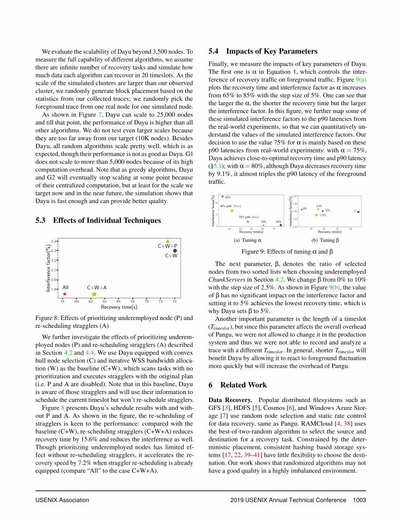
5.4 Impacts of Key ParametersFinally, we measure the impacts of key parameters of Dayu.The first one is α in Equation 1, which controls the inter-ference of recovery traffic on foreground traffic. Figure 9(a)plots the recovery time and interference factor as α increasesfrom 65% to 85% with the step size of 5%. One can see thatthe larger the α, the shorter the recovery time but the largerthe interference factor. In this figure, we further map some ofthese simulated interference factors to the p90 latencies fromthe real-world experiments, so that we can quantitatively un-derstand the values of the simulated interference factors. Ourdecision to use the value 75% for α is mainly based on thesep90 latencies from real-world experiments: with α = 75%,Dayu achieves close-to-optimal recovery time and p90 latency(§5.1); with α= 80%, although Dayu decreases recovery timeby 9.1%, it almost triples the p90 latency of the foregroundtraffic.

50 55 60 65 70Recovery time(s)

0

5

10

Inte

rfer

ence

fact

or(%

)

65%70%

75% (p90: 6ms)

80% (p90: 17ms)

85%

(a) Tuning α

59 60 61 62Recovery time(s)

1.83

1.84

1.85

1.86

1.87

Inte

rfer

ence

fact

or(%

)

0

2.5%5%

7.5%

10%

(b) Tuning β

Figure 9: Effects of tuning α and β

The next parameter, β, denotes the ratio of selectednodes from two sorted lists when choosing underemployedChunkServers in Section 4.2. We change β from 0% to 10%with the step size of 2.5%. As shown in Figure 9(b), the valueof β has no significant impact on the interference factor andsetting it to 5% achieves the lowest recovery time, which iswhy Dayu sets β to 5%.

Another important parameter is the length of a timeslot(Ttimeslot ), but since this parameter affects the overall overheadof Pangu, we were not allowed to change it in the productionsystem and thus we were not able to record and analyze atrace with a different Ttimeslot . In general, shorter Ttimeslot willbenefit Dayu by allowing it to react to foreground fluctuationmore quickly but will increase the overhead of Pangu.

6 Related Work

Data Recovery. Popular distributed filesystems such asGFS [3], HDFS [5], Cosmos [6], and Windows Azure Stor-age [7] use random node selection and static rate controlfor data recovery, same as Pangu. RAMCloud [4, 38] usesthe best-of-two-random algorithm to select the source anddestination for a recovery task. Constrained by the deter-ministic placement, consistent hashing based storage sys-tems [17, 22, 39–41] have little flexibility to choose the desti-nation. Our work shows that randomized algorithms may nothave a good quality in a highly imbalanced environment.


Some works improve data recovery in erasure-coded stor-age, by accelerating recovery of one failed block [31, 42, 43]or designing new recovery-efficient codes [44–47]. ApplyingDayu to erasure-coded storage is our future work.

Data migration. Data recovery can be viewed as a subtopicof data migration. A number of distributed filesystems [3, 5]trigger data migration with a simple strategy or even manu-ally (e.g., running HDFS balancer [48]). Mirador [34] uses apriority queue to greedily migrate data objects according topre-defined rules. However, experiments in [34] report it doesnot scale well due to its greedy algorithm. Curator [49] uses areinforcement learning solution to determine when to start amigration task, but it does not choose sources and destinationsfor data migration. DH-HDFS [35] utilizes MILP solver tomanage migration of large scale storage system, but for ourproblem, MILP is too slow.

Constrained data placement strategies. Besides consis-tent hashing based storage systems [17, 22, 39–41], there areother systems restricting the data placement. Facebook [50]modifies native HDFS to constrain the placement of blockreplicas into smaller node groups (i.e., with a smaller scatterwidth), reducing the probability of losing data due to simulta-neous node failures. With a fixed scatter width, CopySets [51]and Tiered Replication [52] further try to minimize the num-ber of the distinct copysets in the whole system to reduce theprobability of data loss due to correlated node failures. Weplan to investigate the applicability and effectiveness of Dayuon these strategies in the future.

Large scale scheduling. Many large-scale computationplatforms need to schedule computation tasks, which is sim-ilar to schedule recovery tasks in Dayu. Most centralizedschedulers [53, 54] have poor computation performance ata large scale, and thus distributed schedulers are widely dis-cussed [36, 55, 56]. However, due to the lack of coordinationand the latest state, these schedulers often fail to generatehigh quality decisions [37]. Firmament [37], a centralizedscheduler, succeeds to scale to a 12500-node cluster [57] , butexperiments in [37, 58] report it has limited scalability withmassive short tasks, which is exactly our scenario (§2.2).

7 Conclusion

Our work shows that a centralized scheduler has betterscheduling quality, especially in a dynamic and imbalancedenvironment; its weakness, i.e. relatively low speed comparedto the decentralized schedulers, can be mitigated by differentoptimizations (e.g. timeslot-based scheduling, convex hulloptimization, etc). As a result, it can support a reasonablylarge system we target.

8 Acknowledgment

We thank all reviewers for their insightful comments, andespecially our shepherd Sudarsun Kannan for his guidanceduring our camera-ready preparation. We also thank TianyangJiang for helpful discussions, and Alibaba Cloud for provid-ing us the evaluation cluster. This work was supported bythe National key R&D Program of China under Grant No.2018YFB0203902, and the National Natural Science Founda-tion of China under Grant No. 61672315.

References

[1] Zujie Ren, Weisong Shi, Jian Wan, Feng Cao, and JiangbinLin. Realistic and scalable benchmarking cloud file systems:Practices and lessons from alicloud. IEEE Transactions onParallel and Distributed Systems, 28(3272-3285):1, 2017.

[2] Backblaze. Backblaze Durability is 99.999999999% —And Why It Doesn’t Matter. https://www.backblaze.com/blog/cloud-storage-durability/, 2018. Online; ac-cessed 2018-12-25.

[3] Sanjay Ghemawat, Howard Gobioff, and Shun-Tak Leung. TheGoogle file system. In Proceedings of the 19th ACM Sympo-sium on Operating Systems Principles (SOSP’03), volume 37.ACM, 2003.

[4] Diego Ongaro, Stephen M Rumble, Ryan Stutsman, JohnOusterhout, and Mendel Rosenblum. Fast crash recovery inRAMCloud. In Proceedings of the 23rd ACM Symposium onOperating Systems Principles (SOSP’11), pages 29–41. ACM,2011.

[5] Konstantin Shvachko, Hairong Kuang, Sanjay Radia, andRobert Chansler. The Hadoop distributed file system. InProceedings of 26th IEEE symposium on Mass storage systemsand technologies (MSST’10), pages 1–10. IEEE, 2010.

[6] Ronnie Chaiken, Bob Jenkins, Per-Åke Larson, Bill Ramsey,Darren Shakib, Simon Weaver, and Jingren Zhou. Scope: easyand efficient parallel processing of massive data sets. Proceed-ings of the VLDB Endowment (VLDB’08), 1(2):1265–1276,2008.

[7] Brad Calder, Ju Wang, Aaron Ogus, Niranjan Nilakantan, ArildSkjolsvold, Sam McKelvie, Yikang Xu, Shashwat Srivastav,Jiesheng Wu, Huseyin Simitci, et al. Windows Azure Storage:a highly available cloud storage service with strong consis-tency. In Proceedings of the Twenty-Third ACM Symposiumon Operating Systems Principles (SOSP’17), pages 143–157.ACM, 2011.

[8] Fay Chang, Jeffrey Dean, Sanjay Ghemawat, Wilson C Hsieh,Deborah A Wallach, Mike Burrows, Tushar Chandra, AndrewFikes, and Robert E Gruber. Bigtable: A distributed storagesystem for structured data. ACM Transactions on ComputerSystems (TOCS), 26(2):4, 2008.


https://www.backblaze.com/blog/cloud-storage-durability/

https://www.backblaze.com/blog/cloud-storage-durability/

[9] Andrea W Richa, M Mitzenmacher, and R Sitaraman. Thepower of two random choices: A survey of techniques andresults. Combinatorial Optimization, 9:255–304, 2001.

[10] Yuchao Zhang, Junchen Jiang, Ke Xu, Xiaohui Nie, Martin JReed, Haiyang Wang, Guang Yao, Miao Zhang, and Kai Chen.BDS: a centralized near-optimal overlay network for inter-datacenter data replication. In Proceedings of the ThirteenthEuropean Conference on Computer Systems (Eurosys’18),pages 10:1–10:14. ACM, 2018.

[11] Jun Woo Park, Alexey Tumanov, Angela Jiang, Michael AKozuch, and Gregory R Ganger. 3Sigma: distribution-basedcluster scheduling for runtime uncertainty. In Proceedingsof the Thirteenth European Conference on Computer Systems(Eurosys’18), page 2. ACM, 2018.

[12] Alexey Tumanov, Timothy Zhu, Jun Woo Park, Michael AKozuch, Mor Harchol-Balter, and Gregory R Ganger.TetriSched: global rescheduling with adaptive plan-aheadin dynamic heterogeneous clusters. In Proceedings of theEleventh European Conference on Computer Systems (Eurosys’16), page 35. ACM, 2016.

[13] Mark de Berg, Otfried Cheong, Marc van Kreveld, and MarkOvermars. Computational geometry: algorithms and applica-tions. Springer-Verlag TELOS, 2008.

[14] Mosharaf Chowdhury, Matei Zaharia, Justin Ma, Michael I.Jordan, and Ion Stoica. Managing data transfers in computerclusters with Orchestra. In Proceedings of the ACM SIGCOMM2011 Conference on Applications, technologies, architectures,and protocols for computer communication (SIGCOMM’11),pages 98–109, New York, NY, USA, 2011. ACM.

[15] James C Corbett, Jeffrey Dean, Michael Epstein, Andrew Fikes,Christopher Frost, Jeffrey John Furman, Sanjay Ghemawat,Andrey Gubarev, Christopher Heiser, Peter Hochschild, et al.Spanner: Google’s globally distributed database. ACM Trans-actions on Computer Systems (TOCS), 31(3):8, 2013.

[16] Apache. HDFS Federation. https://hadoop.apache.org/docs/stable/hadoop-project-dist/hadoop-hdfs/Federation.html, 2018. Online; accessed 2018-04-16.

[17] Sage A. Weil, Scott A. Brandt, Ethan L. Miller, DarrellD. E. Long, and Carlos Maltzahn. Ceph: A scalable, high-performance distributed file system. In Proceedings of the7th USENIX Symposium on Operating Systems Design andImplementation (OSDI ’06), pages 307–320, 2006.

[18] Albert Greenberg, James R Hamilton, Navendu Jain, SrikanthKandula, Changhoon Kim, Parantap Lahiri, David A Maltz,Parveen Patel, and Sudipta Sengupta. VL2: a scalable andflexible data center network. In Proceedings of the ACM SIG-COMM 2009 conference on Applications, technologies, ar-chitectures, and protocols for computer communication (SIG-COMM’09), volume 39, pages 51–62. ACM, 2009.

[19] Albert Greenberg, Parantap Lahiri, David A Maltz, ParveenPatel, and Sudipta Sengupta. Towards a next generation data

center architecture: scalability and commoditization. In Pro-ceedings of the ACM workshop on Programmable routers forextensible services of tomorrow (PRESTO’08), pages 57–62.ACM, 2008.

[20] Radhika Niranjan Mysore, Andreas Pamboris, Nathan Farring-ton, Nelson Huang, Pardis Miri, Sivasankar Radhakrishnan,Vikram Subramanya, and Amin Vahdat. Portland: a scalablefault-tolerant layer 2 data center network fabric. In Proceed-ings of the ACM SIGCOMM 2009 conference on Applications,technologies, architectures, and protocols for computer com-munication (SIGCOMM’09), volume 39, pages 39–50. ACM,2009.

[21] Mohammad Al-Fares, Alexander Loukissas, and Amin Vahdat.A scalable, commodity data center network architecture. InProceedings of the ACM SIGCOMM 2008 conference on Ap-plications, technologies, architectures, and protocols for com-puter communication (SIGCOMM’08), volume 38, pages 63–74. ACM, 2008.

[22] Giuseppe DeCandia, Deniz Hastorun, Madan Jampani, Gu-navardhan Kakulapati, Avinash Lakshman, Alex Pilchin,Swaminathan Sivasubramanian, Peter Vosshall, and WernerVogels. Dynamo: Amazon’s highly available key-value store.In Proceedings of the 21st ACM Symposium on Operating Sys-tems Principles (SOSP’07), volume 41, pages 205–220. ACM,2007.

[23] Thomas H Cormen, Charles E Leiserson, Ronald L Rivest, andClifford Stein. Introduction to algorithms. MIT press, 2009.

[24] Jeffrey Dean and Sanjay Ghemawat. MapReduce: simpli-fied data processing on large clusters. Proceedings of the 6thConference on Symposium on Opearting Systems Design andImplementation (OSDI’04), 51(1):107–113, 2004.

[25] Haryadi S. Gunawi, Riza O. Suminto, Russell Sears, CaseyGolliher, Swaminathan Sundararaman, Xing Lin, Tim Emami,Weiguang Sheng, Nematollah Bidokhti, Caitie McCaffrey,Gary Grider, Parks M. Fields, Kevin Harms, Robert B. Ross,Andree Jacobson, Robert Ricci, Kirk Webb, Peter Alvaro, H. Bi-rali Runesha, Mingzhe Hao, and Huaicheng Li. Fail-slow atscale: Evidence of hardware performance faults in large pro-duction systems. In 16th USENIX Conference on File andStorage Technologies (FAST’18), pages 1–14, Oakland, CA,2018. USENIX Association.

[26] Thanh Do, Mingzhe Hao, Tanakorn Leesatapornwongsa,Tiratat Patana-anake, and Haryadi S. Gunawi. Limplock: Un-derstanding the impact of limpware on scale-out cloud systems.In Proceedings of the 4th Annual Symposium on Cloud Com-puting (SOCC’13), pages 14:1–14:14, New York, NY, USA,2013. ACM.

[27] Peng Huang, Chuanxiong Guo, Jacob R. Lorch, Lidong Zhou,and Yingnong Dang. Capturing and enhancing in Situ systemobservability for failure detection. In 13th USENIX Symposiumon Operating Systems Design and Implementation (OSDI’18),pages 1–16, Carlsbad, CA, 2018. USENIX Association.


https://hadoop.apache.org/docs/stable/hadoop-project-dist/hadoop-hdfs/Federation.html



[28] Mosharaf Chowdhury, Srikanth Kandula, and Ion Stoica. Lever-aging endpoint flexibility in data-intensive clusters. In Proceed-ings of the ACM SIGCOMM 2013 Conference on Applications,technologies, architectures, and protocols for computer commu-nication (SIGCOMM’13), volume 43, pages 231–242. ACM,2013.

[29] Mohammad Al-Fares, Sivasankar Radhakrishnan, BarathRaghavan, Nelson Huang, and Amin Vahdat. Hedera: Dynamicflow scheduling for data center networks. In Proceedings of the7th USENIX Conference on Networked Systems Design and Im-plementation (NSDI’10), Berkeley, CA, USA, 2010. USENIXAssociation.

[30] Chi-Yao Hong, Matthew Caesar, and P Godfrey. Finishingflows quickly with preemptive scheduling. In Proceedings ofthe ACM SIGCOMM 2012 conference on Applications, tech-nologies, architectures, and protocols for computer communi-cation (SIGCOMM’12), pages 127–138. ACM, 2012.

[31] Zhirong Shen, Jiwu Shu, and Patrick PC Lee. Reconsideringsingle failure recovery in clustered file systems. In Proceed-ings of 46th Annual IEEE/IFIP International Conference onDependable Systems and Networks (DSN ’16), pages 323–334.IEEE, 2016.

[32] Subrata Mitra, Rajesh Panta, Moo-Ryong Ra, and SaurabhBagchi. Partial-parallel-repair (ppr): a distributed techniquefor repairing erasure coded storage. In Proceedings of theEleventh European Conference on Computer Systems (Eu-rosys’16), page 30. ACM, 2016.

[33] Gurobi. Gurobi 8.0. URL:http://www.gurobi.com, 2018.Online; accessed 2018-12-25.

[34] Jake Wires and Andrew Warfield. Mirador: An active controlplane for datacenter storage. In Proceedings of 15th USENIXConference on File and Storage Technologies (FAST’17), pages213–228, Santa Clara, CA, 2017. USENIX Association.

[35] Pulkit A. Misra, Inigo Goiri, Jason Kace, and Ricardo Bian-chini. Scaling distributed file systems in resource-harvestingdatacenters. In Proceedings of 2017 USENIX Annual TechnicalConference (ATC’17), pages 799–811, Santa Clara, CA, 2017.USENIX Association.

[36] Kay Ousterhout, Patrick Wendell, Matei Zaharia, and Ion Sto-ica. Sparrow: Distributed, low latency scheduling. In Pro-ceedings of the Twenty-Fourth ACM Symposium on OperatingSystems Principles, SOSP ’13, pages 69–84, New York, NY,USA, 2013. ACM.

[37] Ionel Gog, Malte Schwarzkopf, Adam Gleave, Robert N. M.Watson, and Steven Hand. Firmament: Fast, centralized clusterscheduling at scale. In Proceedings of 12th USENIX Sym-posium on Operating Systems Design and Implementation(OSDI’16), pages 99–115, Savannah, GA, 2016. USENIX As-sociation.

[38] Ryan Scott Stutsman. Durability and crash recovery in dis-tributed in-memory storage systems. PhD thesis, StanfordUniversity, 2013.

[39] Edmund B Nightingale, Jeremy Elson, Jinliang Fan, Owen SHofmann, Jon Howell, and Yutaka Suzue. Flat datacenterstorage. In Proceedings of the 10th USENIX Symposium onOperating Systems Design and Implementation (OSDI’12),pages 1–15, 2012.

[40] Gluster. GlusterFS documention. URL:https://docs.gluster.org/en/latest/, 2018. Online; accessed 2018-12-25.

[41] Ion Stoica, Robert Morris, David Karger, M Frans Kaashoek,and Hari Balakrishnan. Chord: A scalable peer-to-peer lookupservice for internet applications. Proceedings of the ACMSIGCOMM 2001 conference on Applications, technologies, ar-chitectures, and protocols for computer communication (SIG-COMM’01), 31(4):149–160, 2001.

[42] Runhui Li, Xiaolu Li, Patrick PC Lee, and Qun Huang. Repairpipelining for erasure-coded storage. In Proceedings of the2017 USENIX Annual Technical Conference (ATC’17), pages567–579, 2017.

[43] Subrata Mitra, Rajesh Panta, Moo-Ryong Ra, and SaurabhBagchi. Partial-parallel-repair (PPR): a distributed techniquefor repairing erasure coded storage. In Proceedings of theEleventh European Conference on Computer Systems (Eu-rosys’16), page 30. ACM, 2016.

[44] Alexandros G Dimakis, P Brighten Godfrey, Yunnan Wu, Mar-tin J Wainwright, and Kannan Ramchandran. Network codingfor distributed storage systems. IEEE Transactions on Infor-mation Theory, 56(9):4539–4551, 2010.

[45] KV Rashmi, Preetum Nakkiran, Jingyan Wang, Nihar B Shah,and Kannan Ramchandran. Having your cake and eating it too:Jointly optimal erasure codes for I/O, storage, and network-bandwidth. In Proceedings of 13th USENIX Conference onFile and Storage Technologies (FAST’15), pages 81–94, 2015.

[46] Myna Vajha, Vinayak Ramkumar, Bhagyashree Puranik,Ganesh Kini, Elita Lobo, Birenjith Sasidharan, P Vijay Kumar,Alexandar Barg, Min Ye, Srinivasan Narayanamurthy, et al.Clay codes: Moulding MDS codes to yield an MSR code. InProceedings of 16th USENIX Conference on File and StorageTechnologies (FAST’18), volume 2018, pages 139–154, 2018.

[47] Min Ye and Alexander Barg. Explicit constructions of optimal-access MDS codes with nearly optimal sub-packetization.IEEE Transactions on Information Theory, 63(10):6307–6317,2017.

[48] Apache. HDFS Balancer Command. URL:https://hadoop.apache.org/docs/r2.7.2/hadoop-project-dist/hadoop-hdfs/HDFSCommands.html, 2019. Online; accessed2019-01-10.

[49] Ignacio Cano, Srinivas Aiyar, Varun Arora, Manosiz Bhat-tacharyya, Akhilesh Chaganti, Chern Cheah, Brent Chun,Karan Gupta, Vinayak Khot, and Arvind Krishnamurthy. Cu-rator: Self-managing storage for enterprise clusters. In Pro-ceedings of 14th USENIX Symposium on Networked SystemsDesign and Implementation (NSDI’17), pages 51–66, Boston,MA, 2017. USENIX Association.


URL: http://www. gurobi. com

URL: https://docs.gluster.org/en/latest/

URL: https://docs.gluster.org/en/latest/

URL: https://hadoop.apache.org/docs/r2.7.2/hadoop-project-dist/hadoop-hdfs/HDFSCommands.html



[50] Dhruba Borthakur, Jonathan Gray, Joydeep Sen Sarma, Kan-nan Muthukkaruppan, Nicolas Spiegelberg, Hairong Kuang,Karthik Ranganathan, Dmytro Molkov, Aravind Menon,Samuel Rash, et al. Apache hadoop goes realtime at facebook.In Proceedings of the 2011 ACM SIGMOD International Con-ference on Management of data (SIGMOD’11), pages 1071–1080. ACM, 2011.

[51] Asaf Cidon, Stephen Rumble, Ryan Stutsman, Sachin Katti,John Ousterhout, and Mendel Rosenblum. Copysets: Reducingthe frequency of data loss in cloud storage. In Proceedingsof the 2013 USENIX Annual Technical Conference (USENIXATC’13), pages 37–48, 2013.

[52] Asaf Cidon, Robert Escriva, Sachin Katti, Mendel Rosenblum,and Emin Gun Sirer. Tiered replication: A cost-effective alter-native to full cluster geo-replication. In 2015 USENIX AnnualTechnical Conference (USENIX ATC’15), pages 31–43, 2015.

[53] Michael Isard, Vijayan Prabhakaran, Jon Currey, Udi Wieder,Kunal Talwar, and Andrew Goldberg. Quincy: Fair schedulingfor distributed computing clusters. In Proceedings of the ACMSIGOPS 22nd symposium on Operating systems principles(SOSP’09), pages 261–276. ACM, 2009.

[54] Benjamin Hindman, Andy Konwinski, Matei Zaharia, Ali Gh-odsi, Anthony D. Joseph, Randy Katz, Scott Shenker, and Ion

Stoica. Mesos: A platform for fine-grained resource sharing inthe data center. In Proceedings of the 8th USENIX Conferenceon Networked Systems Design and Implementation (NSDI’11),NSDI’11, pages 295–308, Berkeley, CA, USA, 2011. USENIXAssociation.

[55] Eric Boutin, Jaliya Ekanayake, Wei Lin, Bing Shi, JingrenZhou, Zhengping Qian, Ming Wu, and Lidong Zhou. Apollo:Scalable and coordinated scheduling for cloud-scale comput-ing. In Proceedings of the 11th USENIX Symposium on Oper-ating Systems Design and Implementation (OSDI’14), pages285–300, Broomfield, CO, 2014. USENIX Association.

[56] Pamela Delgado, Florin Dinu, Anne-Marie Kermarrec, andWilly Zwaenepoel. Hawk: Hybrid datacenter scheduling. InProceedings of the 2015 USENIX Annual Technical Conference(ATC’15), pages 499–510, Santa Clara, CA, 2015. USENIXAssociation.

[57] Charles Reiss, Alexey Tumanov, Gregory R Ganger, Randy HKatz, and Michael A Kozuch. Heterogeneity and dynamicityof clouds at scale: Google trace analysis. In Proceedings ofthe Third ACM Symposium on Cloud Computing (SOCC’12),page 7. ACM, 2012.

[58] Ionel Corneliu Gog. Flexible and efficient computation in largedata centres. PhD thesis, University of Cambridge, 2018.


dayu: fast and low-interference data recovery in very-large … · dayu: fast and low-interference...

Documents