dealing with uncertainty in safety function failure …

Rev 0, 24th April 2019 © 2019 I&E Systems Pty Ltd 1

DEALING WITH UNCERTAINTY IN SAFETY FUNCTION FAILURE RATES

I&E Systems Pty Ltd ACN 069 813 958

Mirek Generowicz

FS Senior Expert (TÜV Rheinland #183/12)

I

Dealing with Uncertainty in Failure Rates


CONTENTS A New Requirement to Assess Uncertainties .......................................................................... 3

Summary ............................................................................................................................... 3

Failure Rate Data Sources ...................................................................................................... 5

Characterising Failures ........................................................................................................... 5

Measuring Failure Performance ............................................................................................. 5

Characterising failure rate .................................................................................................................. 5

Distinguishing MTBF from Useful Service Life ................................................................................... 6

Recording and analysing failures ........................................................................................................ 6

Purely random failure ......................................................................................................................... 6

Failure rate with no failures ................................................................................................................ 8

Systematic failure and quasi-random failure ...................................................................................... 8

Assessing whether failure rates are constant ..................................................................................... 9

Failure Rate Uncertainty – Prior Use Data ........................................................................................ 10

Failure Rate Uncertainty – Industry-wide Data ................................................................................ 10

Failure Rate Uncertainty – Manufacturers’ Data .............................................................................. 11

Summary of Uncertainty in Reliability Data Sources ........................................................................ 11

Uncertainty in Probability of Failure on Demand .................................................................. 12

Directly Proportional to Failure Rate ................................................................................................ 12

Uncertainty and Monte Carlo Simulations ....................................................................................... 12

Dealing with Unavoidable Uncertainty ............................................................................................. 12

Visualising Uncertainty in Probability of Failure on Demand ........................................................... 13

Examples with Data from Prior Use .................................................................................................. 13

Increased confidence level ............................................................................................................... 15

Industry-wide data ............................................................................................................................ 15

Failure Rate Performance Scaling Factor ............................................................................... 16

Maintenance Effectiveness ............................................................................................................... 16

Claiming Credit for Improved Maintenance Effectiveness ............................................................... 18

Conclusions ......................................................................................................................... 19

Accept the uncertainty ..................................................................................................................... 19

Acknowledge the uncertainty ........................................................................................................... 19

Identify the factors that influence uncertainty ................................................................................. 19

References .......................................................................................................................... 21



A New Requirement to Assess Uncertainties Automatic safety functions are designed to achieve risk reduction for hazards in process industries. The risk reduction achieved by a safety function can be estimated by calculating the probability of the function failing on demand.

The second edition of IEC 61511 brought in a new requirement (§11.9.4): ‘reliability data uncertainties shall be assessed and taken into account when calculating the failure measure’.

This leads to some questions:

• What is the uncertainty in the failure rates that we use?

• How should we take the uncertainty into account?

This paper explores the uncertainty that is inescapable in estimating the performance of process sector safety functions. It discusses factors that influence uncertainty in failure performance.

Summary • Uncertainty in reliability data is unavoidable. The wide uncertainty bands in failure rates

have been understood and well documented for at least several decades.

• Estimates of failure probability should have a certainty level of at least 70%. This means that the chance of the failure probability being higher than estimated is unlikely to be more than 30%.

• Failure rates with a certainty level of 70% are readily obtainable from industry-wide sources.

• The 90% uncertainty interval is the band between a certainty level of 5% and a certainty level of 95%. It is usually more than an order of magnitude wide and may span 2 or 3 orders of magnitude. The 90% certainty interval should always be indicated clearly in estimates of failure probability. It can be conveniently stated as a numerical range. For example, we might estimate probability of failure as ≈ 0.002 at a 70% certainty level within a 90% interval ranging from 0.0002 to 0.006.

• If the calculation results are presented in a graphical plot of probability over time, the uncertainty interval can be overlaid on the plot:

FIGURE 1. Graphical representation of uncertainty



• Failure probability estimated with a 95% certainty level can be expected to be around 3 to 4 times higher than an estimate at a 70% certainty level. This means that the worst-case performance will be within about half an order of magnitude of the 70% certainty level estimate.

• This level of uncertainty in performance is acceptable because risk reduction targets are set in orders of magnitude. Risk can only be estimated to within half an order of magnitude at best.

• A safety function can be considered to meet its target dependably if its estimated failure probability is below its performance target by a factor of 3 or more.

• The factors that influence failure performance and uncertainty in failure rate can be controlled through deliberate actions in design, installation and maintenance.

• Failure performance of safety functions can be optimised if necessary by ensuring that:

The equipment is always readily accessible for inspection, testing and maintenance

The design enables complete end-to-end testing

The components are suitable for the intended service conditions

Degraded performance is always detected and corrected within the target for mean time to restoration (MTTR)

Functional failure is prevented through regular monitoring and condition-based repair and renewal.



Failure Rate Data Sources The uncertainty in a failure rate depends on its source. There are three commonly used sources of reliability data:

• Failure rates measured in our own operation, i.e. data from prior use

• Failure rates from industry-wide databases such as OREDA, exida, SINTEF, FARADIP, CCPS

• Failure rates reported by manufacturers or certification agencies.

Characterising Failures Failure rates can be expected to occur vary over time.

Over the useful lifetime of equipment failure rates can increase, decrease or remain reasonably constant. Refer to Nowlan and Heap[1] or to Moubray[2] for detailed explanation of failure patterns.

In the context of safety function performance it is useful to distinguish five types of failure:

• Purely systematic failures

Characterised by a probability of failure that does not change until the systematic faults are found and rectified.

• Early failures (partially systematic)

Characterised by a failure rate that decreases as the causes or faults contributing to the failures are identified and rectified.

• Purely random failures

Characterised by a fixed and constant failure rate that cannot be easily changed.

• Mid-life failures (quasi-random, partially systematic)

Characterised by a failure rate that remains reasonably constant but depends both on the suitability of the sub-system design and on the effectiveness of the maintenance practices.

• End-of-life failures (partially systematic)

Characterised by a failure rate that increases noticeably due to age and/or wear as the equipment approaches the end of its useful service life.

Measuring Failure Performance

Characterising failure rate Equipment failure rates must be measured during operation to determine if they meet the targets assumed during design. Refer to IEC 61511 §5.2.5.3 and §16.2.9.

The average failure rate λ of any type of equipment can be estimated by dividing the number of failures n by the total aggregated time in service T :

𝜆𝜆 ≈𝑛𝑛𝑇𝑇



The failure rate may also be expressed as the mean time between failures, MTBF :

𝑀𝑀𝑇𝑇𝑀𝑀𝑀𝑀 =1𝜆𝜆

Distinguishing MTBF from Useful Service Life The MTBF is not an indication of service lifetime, it is an indication of the failure rate during the useful working life of a device. A ball valve might typically have a MTBF in the region of 100 years, but its useful service life between overhaul (mission time) might be less than 15 or 20 years. The mean lifetime could be around 30 or 40 years if valves are left in service without overhaul until they fail.

Mean lifetime should not be confused with mean time to failure (MTTF ) which is equivalent to MTBF and is applied to non-reparable items.

Recording and analysing failures When any failure is recorded these questions need to be asked:

• What is the apparent cause of the failure?

• Could the failure have been prevented?

• What is the failure rate?

• Is the failure rate acceptable in terms of risk?

• Is the cost of failure prevention justified by the cost of failure consequences?

After 5 or 6 failures have been recorded another question is necessary:

• Is the failure rate increasing, decreasing or remaining constant?

If the investigation of a failure reveals no obvious cause, then the failure might be purely random.

Failures that have a known cause but are not easily preventable could be treated as quasi-random if they occur at a reasonably constant rate

Purely random failure If failures are purely random in nature the measured failure rate will be fixed and constant. The rate depends on some random underlying physical process such as damage from cosmic radiation. The time between failures will follow a normal distribution around a mean.

The notes following IEC 61511-1 §11.9.4 clarify that in calculating probability of failure we need to use failure rates with at least an upper bound confidence of 70% (designated as λ70%).

Confidence levels can be estimated from the mean and standard deviation if many failures have been recorded. If only a few failures have been recorded the estimated rate will be imprecise.



The chi-squared function can be applied to estimate the rate of random failures to any required confidence level and with any number of failures, including zero failures (refer to IEC 61511-2 §A.11.9.4 and to Smith, D. J. ‘Reliability, Maintainability and Risk’ [3]).

The only information needed is the total number of failures recorded of that type and the total aggregated time in service.

𝜆𝜆1−𝛼𝛼 =𝜒𝜒2(𝛼𝛼, 𝜈𝜈)

2𝑇𝑇

χ2 = chi-squared function

α = 1- confidence level

ν = degrees of freedom, in this case = 2.(n + 1)

n = the number of failures in the given time period

T = the number of device-years or device-hours, i.e. the number of devices multiplied by the time in service

The uncertainty in the estimated failure rate can be represented by a 90% confidence interval, ranging from λ5%.to λ95%.

The width of the confidence interval depends only on the number of failures recorded, i.e. the uncertainty in failure rate depends only on the number of failures recorded.

The following chart shows an example with a failure rate of 2 x 10-7 per hour (MTBF 570 years). The error bars are scaled to indicate the 90% confidence interval.

FIGURE 2. Failure rate confidence interval against number of failures recorded

The value of λ70% approaches the true mean λ as more failures are recorded.

The width of the 90% confidence interval becomes significantly narrower when more than 2 or 3 failures have been recorded. The table below summarises the width of the 90% confidence interval expressed in orders of magnitude.



TABLE 1. Failure Rate 90% Confidence Interval Width Against Number of Failures

Number of failures recorded

90% confidence interval λ95% / λ5%

Interval width, orders of magnitude

0 58 1.8 1 13 1.1 3 6 0.8

10 2.7 0.4 30 1.8 0.3

100 1.4 0.1

One order of magnitude corresponds with a ratio of 10:1 between the upper and lower limits. Half an order of magnitude is a ratio of approximately 3:1 because 100.5 ≈ 3.

Failure rate with no failures We can still estimate a failure rate even though no failures have been measured because the total time in service provides information about limiting values for failure rate.

In the example shown in FIGURE 2 we have a population of 100 devices that have operated for 5 years without failure. The MTBF can be estimated as around 400 years (2.5 x 10-7 per hour) with a 70% confidence level.

If the first failure occurs shortly after 5 years of service the simple average failure rate is one failure in 500 device-years, but too few failures have been recorded for this to be a precise estimate. The chi-squared function allows us to estimate the MTBF as 230 years (5 x 10-7 per hour) with a 70% confidence level.

Systematic failure and quasi-random failure Strictly speaking, a normal distribution and the chi-squared function apply only if the failures are purely random.

Faults in design, manufacture, installation, commissioning operation or maintenance are categorised as systematic. Systematic failures can be gradually eliminated as the faults are progressively discovered and remedied.

In practice some systematic failures may never be completely eliminated. The amount of effort put into preventing failures needs to be in proportion to the cost of the consequences of failure.

The rate at which failures occur can be measured, but it needs to be understood that the rate is not a fixed constant. If the overall cost of the failures is acceptable (including consideration of safety) then the measured failure rate may be acceptable.

Systematic failures are characterised by probability, not by failure rate. The rate of failures can still be measured but there is no underlying mechanism that would lead to a fixed failure rate.

The failure rate usually depends strongly on the effectiveness of the design, operation and maintenance in preventing failure. The rate can be expected to change over time as the conditions change and as the people in the organisation are changed.

The critical question is then whether the failure rate is increasing, decreasing or remaining reasonably constant. If the rate is reasonably constant the failures can be treated as quasi-random.



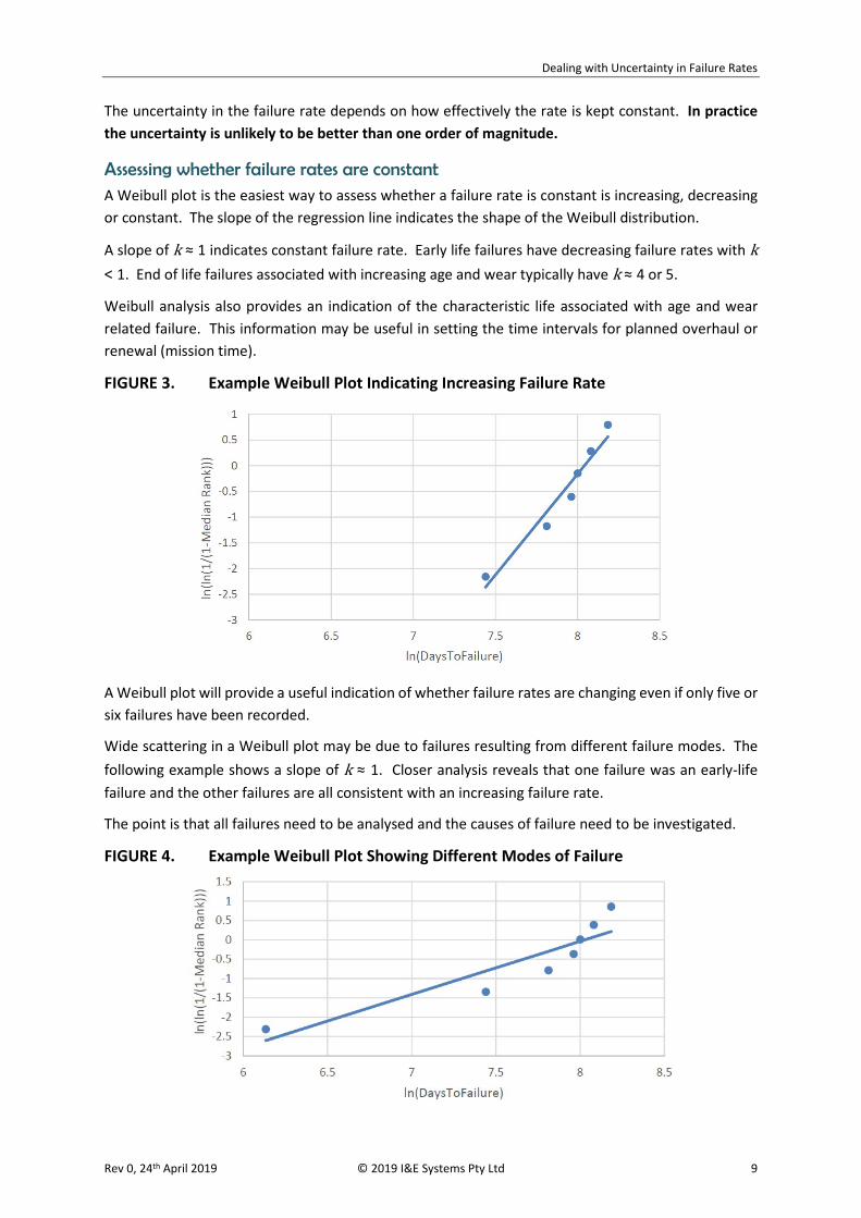
The uncertainty in the failure rate depends on how effectively the rate is kept constant. In practice the uncertainty is unlikely to be better than one order of magnitude.

Assessing whether failure rates are constant A Weibull plot is the easiest way to assess whether a failure rate is constant is increasing, decreasing or constant. The slope of the regression line indicates the shape of the Weibull distribution.

A slope of k ≈ 1 indicates constant failure rate. Early life failures have decreasing failure rates with k < 1. End of life failures associated with increasing age and wear typically have k ≈ 4 or 5.

Weibull analysis also provides an indication of the characteristic life associated with age and wear related failure. This information may be useful in setting the time intervals for planned overhaul or renewal (mission time).

FIGURE 3. Example Weibull Plot Indicating Increasing Failure Rate

A Weibull plot will provide a useful indication of whether failure rates are changing even if only five or six failures have been recorded.

Wide scattering in a Weibull plot may be due to failures resulting from different failure modes. The following example shows a slope of k ≈ 1. Closer analysis reveals that one failure was an early-life failure and the other failures are all consistent with an increasing failure rate.

The point is that all failures need to be analysed and the causes of failure need to be investigated.

FIGURE 4. Example Weibull Plot Showing Different Modes of Failure



Note that a particular failure mode may only affect a subset of devices in a population. For example, failures through contamination or corrosion might affect 20 devices out of a population of 100. The characteristic life associated with failures caused by contamination might be in the order of 8 years even though the overall mean useful lifetime of the devices might be more than 30 years.

Failure Rate Uncertainty – Prior Use Data Analysis using the chi-squared function suggests that if more than two failures have been recorded the 90% confidence interval in failure rate spans less than one order of magnitude. If ten or more failures have been recorded the interval would span less than half an order of magnitude.

This would be true if all of the failures were purely random and characterised by a fixed and constant rate. ISO/TR 12489 clarifies that only purely random failures can be expected to occur at fixed constant rates.

Purely random failures are sudden and complete failures that occur without warning. This type of failure cannot be predicted by examining an item. It has no obvious cause and cannot be prevented.

Purely random failure usually only affects electronic devices such as logic solvers and sensor electronics.

Sensor and final element subsystems usually include components that are not electronic. Most failures of sensor and final element subsystems are predictable and preventable to at least some extent. The failure rates are not fixed. The rates depend on the level of effort put into detecting deterioration and preventing eventual failure.

The uncertainty in failure rates from prior use data should never be expected to be much better than one order of magnitude because in practice failures are never purely random.

Failure Rate Uncertainty – Industry-wide Data The ‘Offshore and Onshore Reliability Data Handbook’ (OREDA) [4,5] summarises failure rates reported by a consortium of petroleum producers.

The chi-squared function cannot be applied to multi-sample sets because the failures are almost never purely random and different producers measure different failure rates.

Failure rates drawn from industry -wide sources such as the exida ‘Safety Equipment Reliability Handbook’ [6,7] or OREDA use uncertainty levels rather than confidence levels. The uncertainty level reflects the proportion of users that achieve a failure rate no higher than the stated value.

OREDA characterises failure rates by mean and standard deviation.

The OREDA statistics show that the reported average failure rates typically vary over more than an order of magnitude between the different producers. The normal distribution cannot be used because the failures are very clearly not random.

Approximately 70% of the reported failure rates might be expected to be less than 0.5 standard deviations above the mean, and the maximum reported failure rate might be expected to be about 2 standard deviations above the mean. These values are for guidance only. Though a standard deviation can be measured we cannot be sure of the shape of the distribution.

OREDA fits gamma probability distributions to model the variation between producers. Upper (95%) and lower (5%) uncertainty limits are inferred from the assumed distributions.

The span between the upper and lower limits represents a 90% uncertainty interval.



The variation in performance between users is evident from the ratio between the upper and lower deciles.

The statistics reported by OREDA suggest that the upper limits of reported failure rates for ESD valves are typically 2 to 3 times higher than a rate that would be representative of at least 70% of users (0.5 standard deviations above the mean). The lower limits of rates are at least 10 times lower than the 70th percentile values. With some taxonomies the lower decile values are more than 30 times lower.

Failure rates based on FMEDA studies by exida are generally consistent with 70th percentile figures from OREDA. Precise comparisons are not possible because of the wide variation in the datasets and in the interpretation and categorisation of failure rates.

The variation in failure rates for ESD valves generally spans more than 2 orders of magnitude. For sensors the variation is generally in the range of about 1 to 1.5 orders of magnitude. Pressure transmitters have the highest variance, spanning 3 orders of magnitude. Temperature sensors have relatively low variance with a span of around 0.7 orders of magnitude.

Failure Rate Uncertainty – Manufacturers’ Data Failure rates reported by manufacturers or reported on SIL certificates are typically 30 to 50 times lower than the 70th percentile rates inferred from OREDA or from exida data.

One of the reasons that the rates are lower is that systematic failures are deliberately excluded from consideration. Manufacturers should not be expected to take accountability for failures that result from misapplication of devices or from lack of preventive maintenance.

Failure rates stated on certificates can be considered as aspirational stretch targets. To achieve such low failure rates will require regular periodic condition monitoring and effective preventive maintenance to address deterioration. It also depends on the device being suitable for the process conditions and environmental conditions.

The failure rates that can be achieved in practice will usually be at least an order of magnitude higher than the rates stated on certificates.

Summary of Uncertainty in Reliability Data Sources David Smith reviewed the confidence interval limits for various data sources in his book ‘Reliability, Maintainability and Risk’ [3]. His results are summarised in the following table:

TABLE 2. Confidence Interval by Data Source (from Smith, D.J.)

Data source 90% confidence interval λ95% / λ5%

Interval width, orders of magnitude

Site specific data 0.3 λ to 3.5 λ 1.1 Industry specific data 0.2 λ to 5 λ 1.4 Generic data 0.1 λ to 8 λ 1.8



Uncertainty in Probability of Failure on Demand

Directly Proportional to Failure Rate In each subsystem of a safety function the probability of failure on demand is approximately directly proportional to the rate of dangerous undetected failures λDU, of the elements irrespective of the architecture.

With a single channel the proportional relationship is clear:

𝑃𝑃𝑀𝑀𝑃𝑃𝐴𝐴𝐴𝐴𝐴𝐴 ≈ 𝜆𝜆𝐷𝐷𝐷𝐷. 𝑇𝑇

2

With any voted architecture the probability of failure is usually dominated by the common cause failure term (unless completely diverse elements are used). The common cause failure term is also directly proportional to rate of dangerous undetected failures λDU:

𝑃𝑃𝑀𝑀𝑃𝑃𝐴𝐴𝐴𝐴𝐴𝐴 ∝ 𝛽𝛽.𝜆𝜆𝐷𝐷𝐷𝐷. 𝑇𝑇

2

The uncertainty interval in the estimated probability of failure on demand is therefore at least as wide as the uncertainty interval in the estimated rate of dangerous undetected failures λDU. We could consider additional uncertainties from variation in β and T but the uncertainty in these factors will not be as significant as the uncertainty in λDU.

Uncertainty and Monte Carlo Simulations There are many factors that each contribute uncertainties to the overall probability of failure of a safety function.

Each sub-system has uncertainty in:

• Dangerous undetected failures λDU • Diagnostic coverage • Common cause failure factor β • Test interval T1 • Mission time TM • Proof test coverage • Mean time to restoration MTTR

Monte Carlo and Markov chain techniques might be proposed to combine the uncertainties from these different contributions. Complex mathematical algorithms such as Monte Carlo are unlikely to improve precision because the causes of uncertainty are mostly systematic rather than purely random.

The level of uncertainty itself is uncertain.

Dealing with Unavoidable Uncertainty Though uncertainty must be acknowledged it can simply be accepted as unavoidable.

Risk assessments are never more precise than half an order of magnitude at best, so the failure probability performance targets have similar imprecision.

The estimated probability of failure of a safety function is only a performance target. It cannot be treated as an invariable physical parameter.

The performance measured during operations can be changed to meet the target by improving the effectiveness of maintenance practices.



The factors that have the strongest influence on probability of failure can all be changed through deliberate action.

Visualising Uncertainty in Probability of Failure on Demand The example below shows the contribution to probability of failure from a 1oo2 pair of actuated valves as final elements. In this example the valves have MTBFDU ≈ 40 years, are subject to annual proof testing with 97% coverage and a mission time of 15 years has been assumed.

FIGURE 5. Example probability of failure plot with no consideration of uncertainty

The effects of the parameters influencing uncertainty can be illustrated by superimposing the 90% confidence interval on the plot.

Examples with Data from Prior Use The first example is of an organisation that has a large volume of data from prior use. At least 10 failures have been measured. Preventable failures have been addressed as far as is practicable. The measured failure rate has remained reasonably constant. The resulting uncertainty interval in failure performance is less than half an order of magnitude wide.



FIGURE 6. Example: Prior Use Claimed, 10 Random Failures, 70% Confidence Level

This should be considered as an ideal scenario that could be achieved with perfect preventive maintenance. Such a narrow uncertainty interval cannot be achieved in practice for several reasons:

• It is rare to find detailed investigation and detailed analysis of all failures. Failure reports contain limited information with descriptions such as ‘Failure mode: broken’, ‘Remedial action: replaced’.

• Constant failure rates are unusual because the failures will have a wide variety of causes

• Maintenance resources and budgets are limited; perfect preventive maintenance is difficult to achieve

If 3 or fewer failures have been are recorded the uncertainty band is wider, even if the estimated value λDU 70% remains unchanged. The uncertainty interval is approximately 0.7 of an order of magnitude wide (a ratio of more than 5 between the upper and lower limits).

FIGURE 7. Example: Prior Use Claimed, 2 or 3 Random Failures, 70% Confidence Level



Increased confidence level If the failure rate is estimated with a 90% confidence level rather than 70% the estimated probability of failure will be closer to the top of the uncertainty interval.

The following example uses exactly the same value for λDU but assumes the confidence level is 90%. The uncertainty interval is the same width but is offset lower with respect to the estimated probability.

FIGURE 8. Example: Prior Use Claimed, 2 or 3 Random Failures, 90% Confidence Level

Industry-wide data If industry-wide failure rate statistics have been used the uncertainty interval can be expected to span about one and half orders of magnitude or more:

FIGURE 9. Example: Industry-wide data, 70% Confidence Level



Failure Rate Performance Scaling Factor Failure rate performance depends largely on the suitability of the design and on the effectiveness of the maintenance in preventing failures. Two main factors limit the failure performance that can be achieved in practice:

• The suitability of the design for the application, for the environment and for the SIL

• Adequate accessibility and resources to enable effective inspection, testing, maintenance and renewal.

The failure rates will vary if the conditions of operation change or if the effectiveness of maintenance practices changes.

If the operating environment remains reasonably constant failure rates can be measured with some level of confidence.

If prior use has been claimed the effectiveness of the operator’s maintenance practices will already be reflected in the measured failure rates. No further scaling is required.

If prior use has not been claimed the failure rates need to be factored to reflect the expected degradation in maintenance effectiveness.

Maintenance Effectiveness Failure rates taken from industry-wide data are selected to represent at least 70% of users.

The OREDA statistics suggest that the upper decile failure rates can be 2 or3 times higher than the 70th percentile failure rates.

The paper titled ‘Quantifying the Impacts of Human Factors on Functional Safety’ [8] presented by Bukowski and Stewart reviews the effect of maintenance practices on field failure data.

The paper concludes ineffective maintenance practices can result in the probability of failure being as much as 4 times higher than for organisations that effectively apply commonly accepted standards of maintenance.

In the example estimates for this paper we have taken a simple heuristic approach to modelling scaling factors for maintenance effectiveness.

TABLE 3. MAINTENANCE SCALING FACTOR OPTIONS

Criteria YES NO

Users with prior use failure data x 1

Is there evidence that degraded performance will always be detected and corrected within MTTR?

x 1 x 2

Will the equipment always be readily accessible for inspection, testing and maintenance?

x 1 x 2

Is there an auditable plan for regular monitoring and condition-based repair and renewal to prevent failure?

x 0.3 x 1



The effect of a x 2 degradation scaling factor is to move the probability plot higher relative to the same uncertainty band. The uncertainty band is based on the unscaled value.

FIGURE 10. Example: Industry-wide data, 70% Confidence Level, Maintenance Scaling Factor x 2

In the worst case a scaling factor of x 4 is applied to the estimated probability of failure. The uncertainty band is still based on the unscaled value, but the top of the uncertainty interval is offset upwards to accommodate the scaled result.

FIGURE 11. Example: Industry-wide data, 70% Confidence Level, Maintenance Scaling Factor x 4



Claiming Credit for Improved Maintenance Effectiveness The standard deviations presented in OREDA statistics suggest that around 40% of operators can achieve failure rates a factor of 3 lower than the 70th percentile rates.

On that basis it could be reasonable to set a target maintenance scaling factor of 0.3 if an auditable and highly effective preventive maintenance programme has been established.

The uncertainty band remains unchanged, but the failure rate performance target can be set at a lower level. The estimated probability of failure is reduced in proportion. In effect this sets an aspirational stretch target for operations and maintenance performance.

FIGURE 12. Example: Industry-wide data, 70% Confidence Level, Maintenance Scaling Factor x 0.3

The plot clearly illustrates the lack of certainty in achieving such a low target.

The statistics show that lower failure rates can be achieved, but until the operator collects a sufficiently large volume of operational experience it might be difficult to justify setting a lower target.

What is a sufficiently large volume of experience? It would have to be large enough to have measured several failures, and all of those failures would have to have been investigated and analysed. There needs to be sufficient evidence to demonstrate that the failure modes are understood and controlled.

All failure rate targets that are assumed in the calculations must be reviewed and accepted by the operators. The operators must be satisfied that the failure rates are feasible given the design and given the resources that will be available for maintenance.



Conclusions

Accept the uncertainty We need to deal with the fact that uncertainty in reliability data is unavoidable.

The uncertainty itself cannot be characterised with precision, but it can be controlled and managed.

Uncertainties in reliability data from industry-wide sources are indeterminate but can be expected to span at least one order of magnitude. Uncertainties may span as much as two or three orders of magnitude.

Failure rates measured in prior use in the user’s own application will have lower uncertainty than industry-wide data, even if only one failure has been measured in operation. Even so, the uncertainty interval will usually span at least an order of magnitude.

Failure probability estimated with a 95% certainty level can be expected to be around 3 to 4 times higher than an estimate at a 70% certainty level.

Therefore, an estimate of failure at a certainty level of 70% will be within about half an order of magnitude of the worst-case performance.

This level of uncertainty in performance is acceptable because risk reduction targets are set in orders of magnitude. Risk can only be estimated to within half an order of magnitude at best.

Acknowledge the uncertainty The wide uncertainty in failure performance must be acknowledged, understood and accepted.

One simple way of taking uncertainties into account is to state the uncertainty explicitly when reporting calculated failure measures. For instance:

TABLE 4. Example uncertainty range for estimated probability of failure

Estimated failure measure (70% confidence level) Uncertainty range

Probability of failure on demand ≈ 0.002 0.0002 to 0.006

Risk reduction factor ≈ 400 100 to 4,000

Overall SIF dangerous failure rate ≈ 4 x 10-7 /h 4 x 10-8 /h to 1 x 10-6 /h

Estimates of failure rates and failure probabilities should never be presented with more than one significant figure of precision.

Uncertainty intervals should always be shown on the graphical plots when they are used to show how probability of failure varies over the system lifetime.

Plots that do not show uncertainty intervals can be misleading because the implied precision is unjustified.

Identify the factors that influence uncertainty The factors that influence failure performance and uncertainty in failure rate can be controlled through deliberate actions in design, installation and maintenance.



Ineffective preventive maintenance has been shown to increase failure rates and probability of failure by at least a factor of 3 (half an order of magnitude).

Performance can be improved if necessary through a robust architectural design that:

• Enables full end-to-end testing (i.e. end-to-end from the measured process parameter through to confirmation that the safe state is achieved)

• Enables deterioration in performance to be detected by regular condition monitoring

• Enables deteriorated equipment to be renewed or replaced before it fails to perform its intended function

• Avoids systematic failures by ensuring that components are suitable for the intended service.

These design principles need to be considered very early in the conceptual design.



References TABLE 5. STANDARDS AND CODES

Number and date Title

IEC 61508: 2010 Functional Safety of electrical/electronic/programmable electronic safety related systems

IEC 61511: 2016 Functional safety — Safety instrumented systems for the process industry sector

ISO/TR 12489: 2013 Petroleum, petrochemical and natural gas industries — Reliability modelling and calculation of safety systems

TABLE 6. REFERENCE DOCUMENTS

Ref Title

1 Nowlan, F.S. & Heap, H. ‘‘Reliability-centred Maintenance’, Springfield Virginia. National Technical Information Service, US Department of Commerce. 1978

2 Moubray, J. ‘Reliability-centred Maintenance’, 2nd Ed. Industrial Press Inc. 1997

3 Smith, D. J. ‘Reliability, Maintainability and Risk’, 6th Ed. Butterworth Heinemann. 2001

4 OREDA Offshore Reliability Data Handbook Volume 1, 5th Ed. SINTEF. 2009

5 OREDA Offshore and Onshore Reliability Data Handbook Volume 1, 6th Ed. SINTEF. 2015

6 exida Safety Equipment Reliability Handbook (‘SERH’), 3rd Ed. 2007

7 exida Safety Equipment Reliability Handbook (‘SERH’), 4th Ed. 2015

8 Bukowski, J.V. and Stewart, L. ‘Quantifying the Impacts of Human Factors on Functional Safety’ exida.

Presented at the American Institute of Chemical Engineers’ 12th Global Congress on Process Safety, Houston, Texas. 2016

9 SINTEF Reliability Prediction Method for Safety Instrumented Systems

PDS Method Handbook. 2013

dealing with uncertainty in safety function failure …

Documents