Decision Support Systems

These slides are a modified version of the slides of the book

“Database System Concepts” (Chapter 18), 5th Ed., McGraw-Hill,

by Silberschatz, Korth and Sudarshan.

Original slides are available at www.db-book.com

1.2

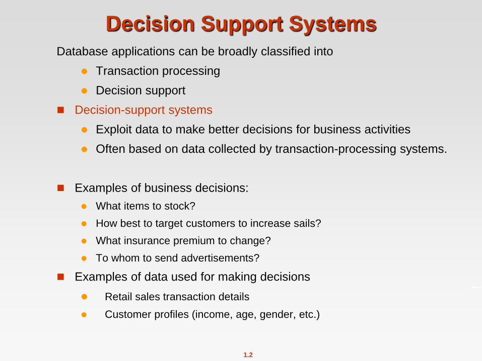
Decision Support Systems Database applications can be broadly classified into

Transaction processing

Decision support

Decision-support systems

Exploit data to make better decisions for business activities

Often based on data collected by transaction-processing systems.

Examples of business decisions:

What items to stock?

How best to target customers to increase sails?

What insurance premium to change?

To whom to send advertisements?

Examples of data used for making decisions

Retail sales transaction details

Customer profiles (income, age, gender, etc.)

1.3

Decision-Support Systems: Overview Issues in storage and retrieval of data in Decision Support Systems

Data analysis

many of the queries are rather complicated, requesting summarised data

on-line answers to queries (On-Line Analytical Processing- OLAP) even if the database is extremely large

certain information cannot be extracted even by using SQL

introduction of specialized tools and SQL extensions to support forms of data analysis SQL:2003 contains additional constructs to support data analysis

Example of data analysis tasks

Retail shop wants to find out :

For each product category and each region, what were the total sales in the last quarter and how do they compare with the same quarter last year

As above, for each product category and each customer category

Statistical analysis of data tools for statistical analysis of data (e.g., : S++) can be interfaced with databases

Statistical analysis is a large field, but not covered here

1.4

Decision-Support Systems: Overview

Data warehouse large companies have diverse sources of data they want to use (generated from multiple divisions, possibly at multiple sites)

We have to build a Data warehouse: gather data from multiple sources and stores it under a unified schema, at a single site.

Data may also be purchased externally

The Data warehouse provides the user a single uniform interface to data

Data mining

Seeks to discover knowledge from data in large databases automatically in the form of statistical rules and patterns Example: on-line book store (database with enormous quantity of information about customers and transactions)

Identify patterns in customers behaviour

Use the patterns to make business decisions

For instance: books that tend to be bought together If a customer buys a book, the book store may suggest other associated books.

1.5

OLTP systems

Transaction Processing Systems - On-Line Transaction Processing

Systems that records information about transactions

ACID properties of transactions

Organizations accumulate a vast amount of information

generated by these systems

Decision Support Systems - On-Line Analytical Processing

Get high level information out of the detailed information

stored in transaction processing systems

Use this information for a variety of decisions

Extremely Large databases

Read-only operations. Periodic updates of data

OLAP systems

1.6

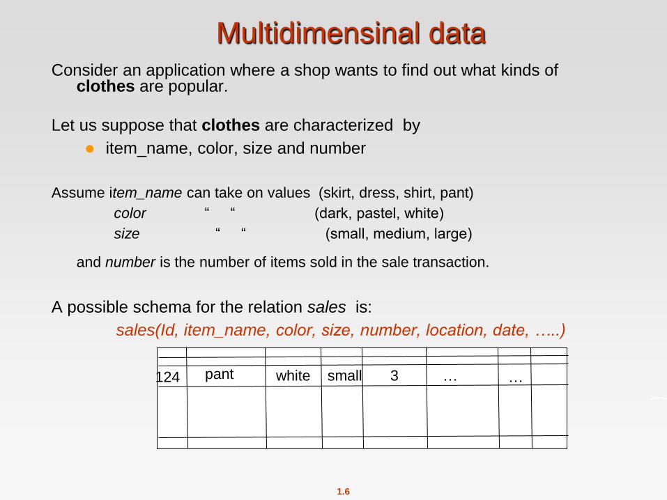
Multidimensinal data Consider an application where a shop wants to find out what kinds of

clothes are popular.

Let us suppose that clothes are characterized by

item_name, color, size and number

Assume item_name can take on values (skirt, dress, shirt, pant)

color “ “ (dark, pastel, white)

size “ “ (small, medium, large) and number is the number of items sold in the sale transaction.

A possible schema for the relation sales is:

sales(Id, item_name, color, size, number, location, date, …..)

3 small white pant 124 … …

1.7

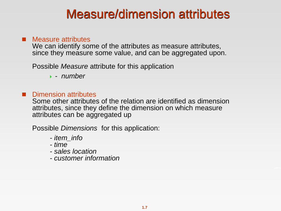
Measure/dimension attributes

Measure attributes We can identify some of the attributes as measure attributes, since they measure some value, and can be aggregated upon. Possible Measure attribute for this application

- number

Dimension attributes Some other attributes of the relation are identified as dimension attributes, since they define the dimension on which measure attributes can be aggregated up Possible Dimensions for this application:

- item_info - time - sales location - customer information

1.8

Multidimensional data

Data that can be modeled as dimension attributes and measure attributes are called multidimensional data.

Techniques to allow analysts to view data in different ways (Interactive analysis of summary information)

Schema for the relation sales used in the examples

sales(item_name, color, size, number)

In the following:

Measure attributes

the attribute number

Dimension attributes

the attributes item_name, color, and size

3 small white pant

…

item_name color size number

1.9

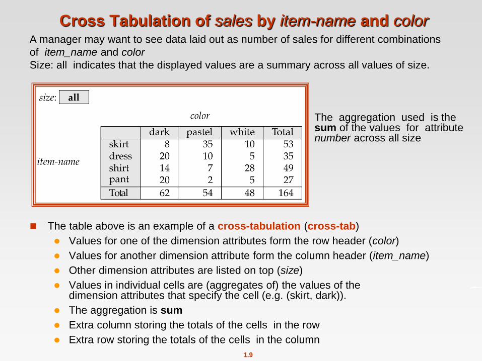
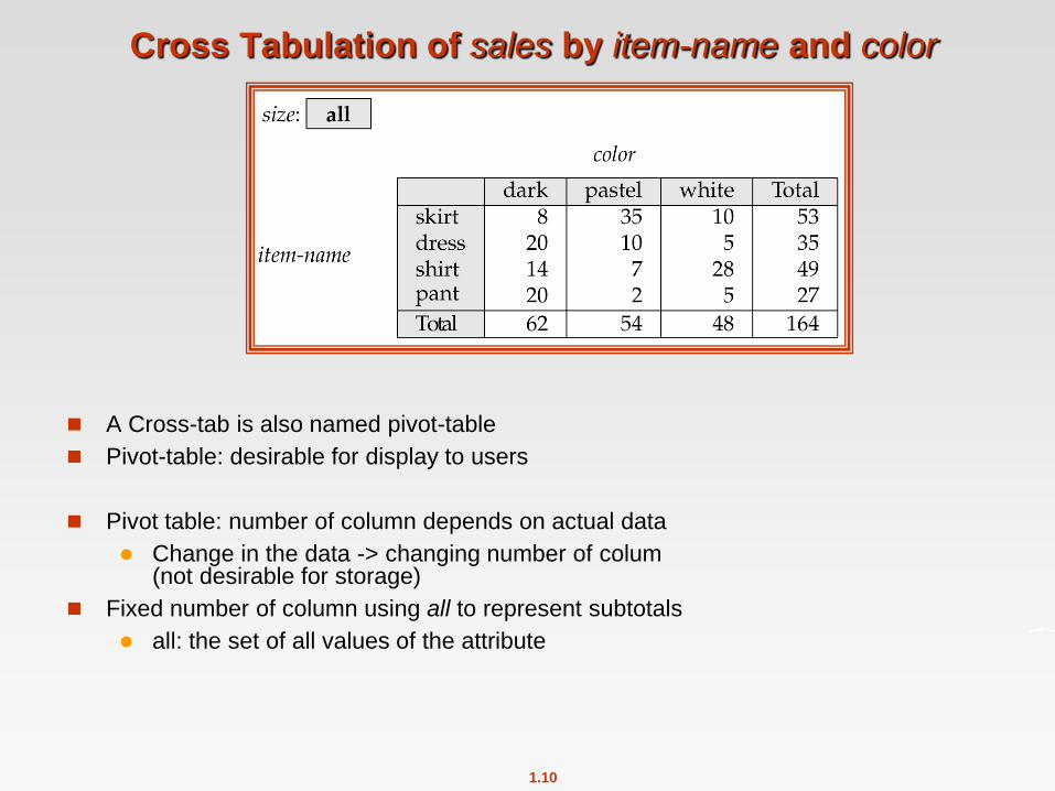
Cross Tabulation of sales by item-name and color

The table above is an example of a cross-tabulation (cross-tab)

Values for one of the dimension attributes form the row header (color)

Values for another dimension attribute form the column header (item_name)

Other dimension attributes are listed on top (size)

Values in individual cells are (aggregates of) the values of the dimension attributes that specify the cell (e.g. (skirt, dark)).

The aggregation is sum

Extra column storing the totals of the cells in the row

Extra row storing the totals of the cells in the column

A manager may want to see data laid out as number of sales for different combinations

of item_name and color

Size: all indicates that the displayed values are a summary across all values of size.

The aggregation used is the sum of the values for attribute number across all size

1.10

Cross Tabulation of sales by item-name and color

A Cross-tab is also named pivot-table

Pivot-table: desirable for display to users

Pivot table: number of column depends on actual data

Change in the data -> changing number of colum (not desirable for storage)

Fixed number of column using all to represent subtotals

all: the set of all values of the attribute

1.11

Relational Representation of Cross-tabs

Cross-tabs can be represented as relations

We use the value all is used to represent aggregates (summary rows or columns)

The SQL:1999 standard actually uses null values in place of all despite confusion with regular null values

tuples with value all for color and size

select item_name, sum (number) from sales

group by item_name

tuples with value all for item_name, colour and size

select sum (number)

from sales

group by;

1.12

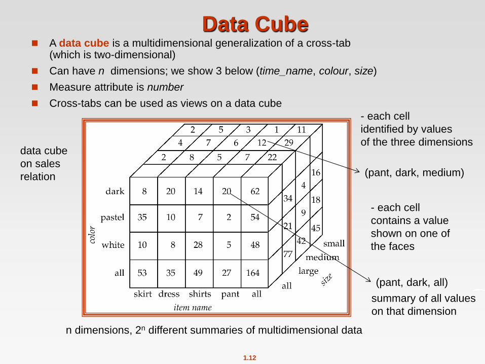
Data Cube A data cube is a multidimensional generalization of a cross-tab

(which is two-dimensional)

Can have n dimensions; we show 3 below (time_name, colour, size)

Measure attribute is number

Cross-tabs can be used as views on a data cube

data cube

on sales

relation

- each cell

identified by values

of the three dimensions

- each cell

contains a value

shown on one of

the faces

(pant, dark, medium)

summary of all values

on that dimension

(pant, dark, all)

n dimensions, 2n different summaries of multidimensional data

1.13

Online Analytical Processing

An OLAP system is an interactive system that permits an analyst to view

different summaries of multidimensional data

Online indicates that an analyst must be able to request new summaries

and get responses on line, and should not be forced to wait for a long

time.

An analyst can look at different cross-tabs on the same data by selecting

the attributes in the cross-tab.

Each cross-tab is a two-dimensional view of a multidimensional

data cube

Functionalities

- Pivoting

- Slicing

- Rollup

- Drill down

1.14

Pivoting

Pivoting: the operation of changing the dimensions used in a cross-tab

1.15

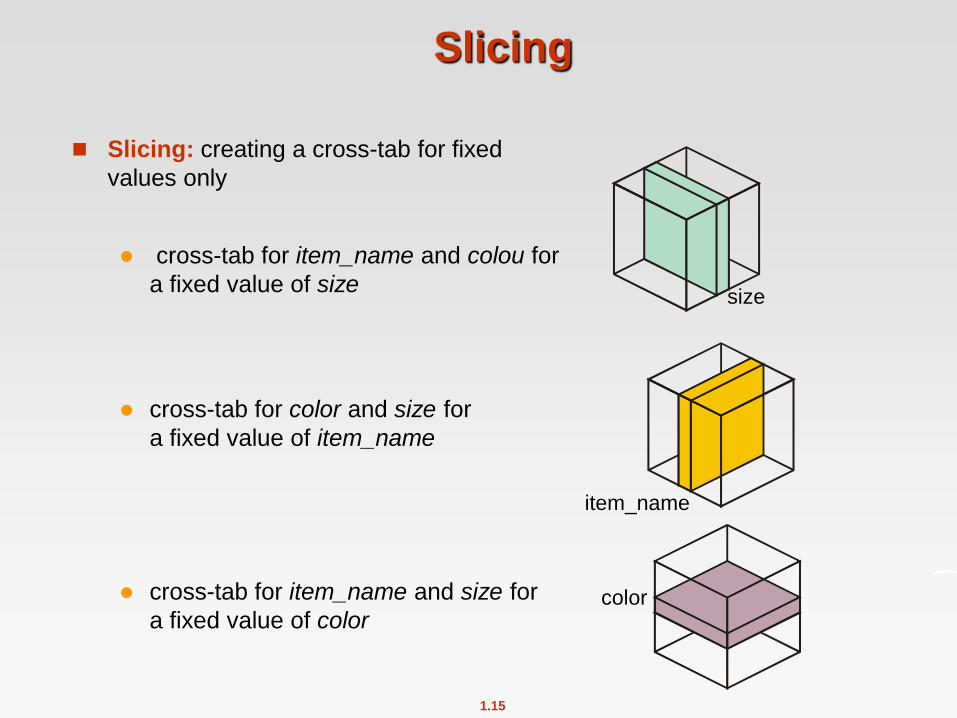
Slicing

Slicing: creating a cross-tab for fixed

values only

cross-tab for item_name and colou for

a fixed value of size

cross-tab for color and size for

a fixed value of item_name

cross-tab for item_name and size for

a fixed value of color

size

color

item_name

1.16

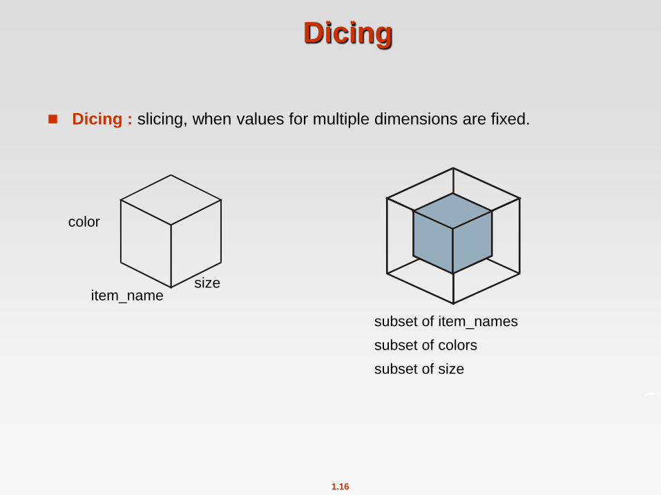
Dicing

Dicing : slicing, when values for multiple dimensions are fixed.

subset of item_names

subset of colors

subset of size

size item_name

color

1.17

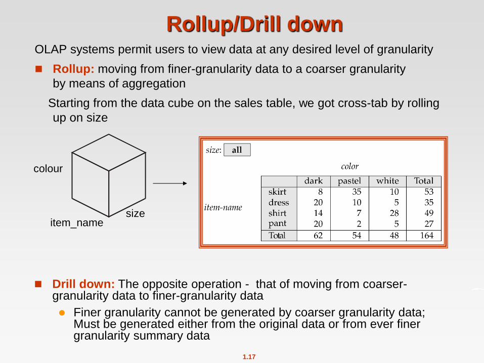
Rollup/Drill down OLAP systems permit users to view data at any desired level of granularity

Rollup: moving from finer-granularity data to a coarser granularity

by means of aggregation

Starting from the data cube on the sales table, we got cross-tab by rolling

up on size

size item_name

colour

Drill down: The opposite operation - that of moving from coarser-granularity data to finer-granularity data

Finer granularity cannot be generated by coarser granularity data; Must be generated either from the original data or from ever finer granularity summary data

1.18

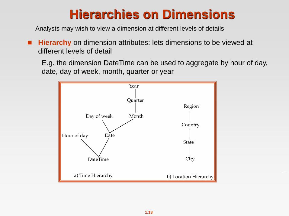
Hierarchies on Dimensions

Hierarchy on dimension attributes: lets dimensions to be viewed at

different levels of detail

E.g. the dimension DateTime can be used to aggregate by hour of day,

date, day of week, month, quarter or year

Analysts may wish to view a dimension at different levels of details

1.19

Cross Tabulation With Hierarchy

on item-name

Cross-tabs can be easily extended to deal with hierarchies

- Can drill down or roll up on a hierarchy

Assume clothes are grouped by category

(menswear and womenswear):

category lies above item_name

Different levels are shown in the same cross-tab

Analyst interested in viewing sales of clothes divides as menswear and

womenswear

category

item_name

cross- tabulation of sales for hierarchy on item_name

1.20

OLAP Implementation

The earliest OLAP systems used multidimensional arrays in memory to

store data cubes, and are referred to as multidimensional OLAP

(MOLAP) systems.

OLAP implementations using only relational database features are called

relational OLAP (ROLAP) systems

Hybrid systems, which store some summaries in memory and store the

base data and other summaries in a relational database, are called

hybrid OLAP (HOLAP) systems.

1.21

OLAP Implementation (Cont.) Early OLAP systems precomputed all possible aggregates in order to

provide online response

Space and time requirements for doing so can be very high

2n combinations of group by

It suffices to precompute some aggregates, and compute others on

demand from one of the precomputed aggregates

Can compute aggregate on (item-name, color) from an aggregate

on (item-name, color, size)

– is cheaper than computing it from scratch

SQL standard aggregate functions:

we can compute an aggregate on grouping on a set of attribute A

from an aggregate on grouping on a set of attribute B if A is a subset of

B.

1.22

OLAP Implementation (Cont.) Several optimizations available for computing multiple aggregates

Can compute aggregates on (item-name, color, size),

(item-name, color) and (item-name) using a single sorting

of the base data

The data in a data cube cannot be generated by a single SQL query

using the basic group by constructs, since aggregates are computed for

several different groupings of the dimension attributes

1.23

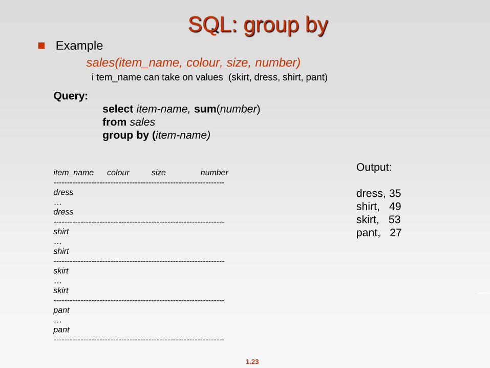
SQL: group by Example

sales(item_name, colour, size, number) i tem_name can take on values (skirt, dress, shirt, pant)

Query:

select item-name, sum(number)

from sales

group by (item-name)

item_name colour size number

---------------------------------------------------------------

dress

…

dress

---------------------------------------------------------------

shirt

…

shirt

---------------------------------------------------------------

skirt

…

skirt

---------------------------------------------------------------

pant

…

pant

---------------------------------------------------------------

Output:

dress, 35

shirt, 49

skirt, 53

pant, 27

1.24

SQL: group by Example

sales(item_name, colour, size, number) color can take on values (dark, pastel, white)

Query:

select item-name, color, sum(number)

from sales

group by (item-name, color)

item_name colour size number

---------------------------------------------------------------

dress dark … ……

…. …

dark

---------------------------------------------

pastel

… …

… pastel

---------------------------------------------

….. white

… ….

dress white

---------------------------------------------------------------

shirt dark

… …

shirt white

---------------------------------------------------------------

………………………………………..

Output:

dress, dark, 20

dress, pastel, 10

dress, white, 5

shirt, dark, 14

shirt, pastel,7

shirt, white, 28

………………

……………

1.25

Extended Aggregation in SQL:1999

Cube construct

The cube operation computes union of group by’s on every subset of the

dimension attributes

E.g. consider the query

select item-name, color, size, sum(number)

from sales

group by cube(item-name, color, size)

This computes the union of eight different groupings of the sales relation:

{ (item-name, color, size), (item-name, color),

(item-name, size), (color, size),

(item-name), (color),

(size), ( )

}

where ( ) denotes an empty group by list.

For each grouping, the result contains the null value for attributes not present

in the grouping.

1.26

Extended Aggregation (Cont.) Rollup construct

The rollup construct generates union on every prefix of specified list of attributes

E.g.

select item-name, color, size, sum(number) from sales group by rollup(item-name, color, size)

Generates union of four groupings:

{ (item-name, color, size),

(item-name, color),

(item-name),

( )

}

1.27

Extended Aggregation (Cont.)

Rollup can be used to generate aggregates at multiple levels of a hierarchy.

E.g., suppose table itemcategory(item-name, category) gives the category of each item. Then

select category, item-name, sum(number) from sales, itemcategory where sales.item-name = itemcategory.item-name group by rollup(category, item-name)

would give a hierarchical summary by item-name and by category.

1.28

Extended Aggregation (Cont.)

Multiple rollups/ cubes

Multiple rollups and cubes can be used in a single group by clause

Each generates set of group by lists, cross product of sets gives overall

set of group by lists

E.g.,

select item-name, color, size, sum(number)

from sales

group by rollup(item-name), rollup(color, size)

generates the groupings

{item-name, ()} X {(color, size), (color), ()}

= { (item-name, color, size), (item-name, color), (item-name),

(color, size), (color), ( ) }

1.29

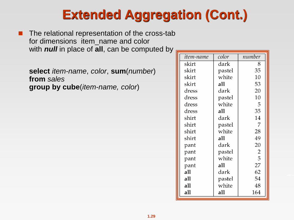
Extended Aggregation (Cont.)

The relational representation of the cross-tab for dimensions item_name and color with null in place of all, can be computed by

select item-name, color, sum(number) from sales group by cube(item-name, color)

1.30

Extended Aggregation (Cont.)

grouping() / decode()

The function grouping() can be applied on an attribute

Returns 1 if the value is a null value representing all, and returns 0 in all other cases in the extra columns

select item-name, color, size, sum(number), grouping(item-name) as item-name-flag, grouping(color) as color-flag, grouping(size) as size-flag, from sales group by cube(item-name, color, size)

Can use the function decode() in the select clause to replace such nulls by a value such as all

E.g. replace item-name in first query by

decode( grouping(item-name), 1, ‘all’, item-name)

1.31

Ranking

Finding the position of a value in a larger set is a common operation

Given a relation

student-marks(student-id, marks)

we wish to assign students a rank in class, based on their total marks

with rank 1 to the student with highest marks, rank 2 to the student

with the next highest marks, and so on

This corresponds to find the rank of each student and this query could be

written partly in SQL and partly in programming language

Rank() construct

The following query gives the rank of each student:

select student-id, rank( ) over (order by marks desc) as s-rank

from student-marks

Ranking is done in conjunction with an order by specification.

1.32

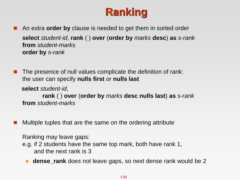
Ranking

An extra order by clause is needed to get them in sorted order

select student-id, rank ( ) over (order by marks desc) as s-rank

from student-marks

order by s-rank

The presence of null values complicate the definition of rank:

the user can specify nulls first or nulls last

select student-id,

rank ( ) over (order by marks desc nulls last) as s-rank

from student-marks

Multiple tuples that are the same on the ordering attribute

Ranking may leave gaps:

e.g. if 2 students have the same top mark, both have rank 1,

and the next rank is 3

dense_rank does not leave gaps, so next dense rank would be 2

1.33

Ranking (Cont.) Ranking can be done within partition of the data.

Assume we have a relation

student_section(student_id, section)

that stores for each student the section in which the student sudies

“Find the rank of students within each section.”

select student-id, section,

rank ( ) over (partition by section order by marks desc)

as sec-rank

from student-marks, student-section

where student-marks.student-id = student-section.student-id

order by section, sec-rank

Multiple rank clauses can occur in a single select clause

Ranking is done after applying group by clause/aggregation if

used together in a select

1.34

Ranking (Cont.)

Other ranking functions:

percent_rank

gives the rank of a tuple as a fraction

If there are n tuples in the partition (the whole set of tuples if no

explicit partition is used), and the rank of the tuple is r,

then the percent_rank is defined as

(r-1)/(n-1)

or null if there is only one tuple in the partition

cume_dist (cumulative distribution)

gives fraction of tuples with preceding values

cume_dist is defined as:

p/n

where p is the number of tuple in the partition with ordering

value preceding or equal to the ordering value of the tuple

and n is the number of tuples in the partition

1.35

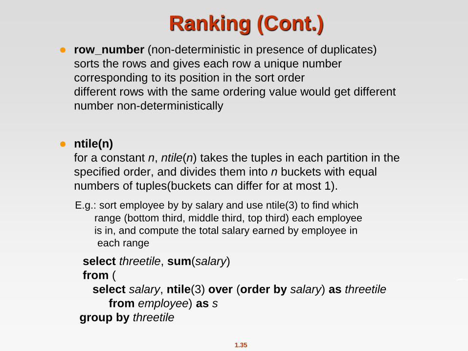
Ranking (Cont.) row_number (non-deterministic in presence of duplicates)

sorts the rows and gives each row a unique number

corresponding to its position in the sort order

different rows with the same ordering value would get different

number non-deterministically

ntile(n)

for a constant n, ntile(n) takes the tuples in each partition in the

specified order, and divides them into n buckets with equal

numbers of tuples(buckets can differ for at most 1).

E.g.: sort employee by by salary and use ntile(3) to find which

range (bottom third, middle third, top third) each employee

is in, and compute the total salary earned by employee in

each range

select threetile, sum(salary)

from (

select salary, ntile(3) over (order by salary) as threetile

from employee) as s

group by threetile

1.36

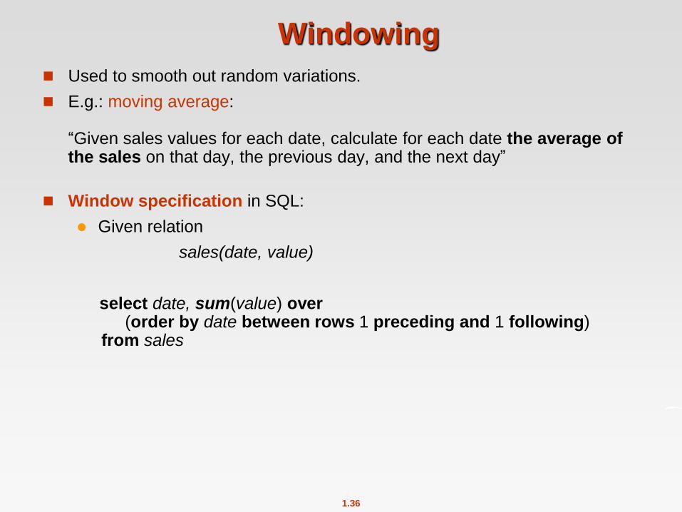
Windowing

Used to smooth out random variations.

E.g.: moving average: “Given sales values for each date, calculate for each date the average of the sales on that day, the previous day, and the next day”

Window specification in SQL:

Given relation

sales(date, value)

select date, sum(value) over (order by date between rows 1 preceding and 1 following) from sales

1.37

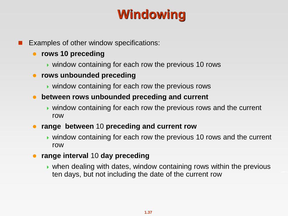
Windowing

Examples of other window specifications:

rows 10 preceding

window containing for each row the previous 10 rows

rows unbounded preceding

window containing for each row the previous rows

between rows unbounded preceding and current

window containing for each row the previous rows and the current row

range between 10 preceding and current row

window containing for each row the previous 10 rows and the current row

range interval 10 day preceding

when dealing with dates, window containing rows within the previous ten days, but not including the date of the current row

1.38

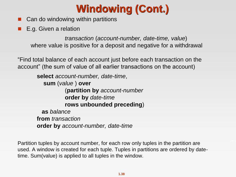
Windowing (Cont.) Can do windowing within partitions

E.g. Given a relation

transaction (account-number, date-time, value)

where value is positive for a deposit and negative for a withdrawal

“Find total balance of each account just before each transaction on the

account” (the sum of value of all earlier transactions on the account)

select account-number, date-time,

sum (value ) over

(partition by account-number

order by date-time

rows unbounded preceding)

as balance

from transaction

order by account-number, date-time

Partition tuples by account number, for each row only tuples in the partition are

used. A window is created for each tuple. Tuples in partitions are ordered by date-

time. Sum(value) is applied to all tuples in the window.