arX

iv:1

901.

0041

9v5

[ec

on.E

M]

27

Jan

2022

Selection and the Distribution of Female

Hourly Wages in the U.S.∗

Ivan Fernandez-Val† Aico van Vuuren‡ Francis Vella§

Franco Peracchi¶

January 28, 2022

Abstract

We analyze the role of selection bias in generating the changes in the

observed distribution of female hourly wages in the United States using CPS

data for the years 1975 to 2020. We account for the selection bias from the

employment decision by modeling the distribution of the number of working

hours and estimating a nonseparable model of wages. We decompose changes

in the wage distribution into composition, structural and selection effects.

Composition effects have increased wages at all quantiles while the impact of

the structural effects varies by time period and quantile. Changes in the role

of selection only appear at the lower quantiles of the wage distribution. The

evidence suggests that there is positive selection in the 1970s which diminishes

until the later 1990s. This reduces wages at lower quantiles and increases wage

inequality. Post 2000 there appears to be an increase in positive sorting which

reduces the selection effects on wage inequality.

Keywords: Wage inequality, wage decompositions, nonseparability, selection bias

JEL-codes: C14, I24, J00

∗ We are grateful to useful comments and suggestions from the editor Chris Taber, two anony-mous referees, Stephane Bonhomme, Chinhui Juhn, Ivana Komunjer, Yona Rubinstein, SamiStouli, and Finis Welch.

† Boston University‡ Gothenburg University and University of Groningen.§ Georgetown University¶University of Rome Tor Vergata

1 Introduction

The dramatic increase in female wage inequality in the United States since the early

1980s (see, for example, Katz and Murphy 1992, Katz and Autor 1999, Lee 1999,

Autor et al. 2008, Acemoglu and Autor 2011, Autor et al. 2016 and Murphy and

Topel 2016) has been accompanied by substantial changes in both female employ-

ment rates and the distribution of their annual hours of work. Given the prominence

that accounting for the selection bias (see Heckman 1974, 1979) from employment

decisions has played in empirical studies of the determinants of female wages it seems

natural to investigate its role in the evolution of wage inequality. This paper exam-

ines the sources of changes in the distribution of female hourly real wage rates in the

United States from 1975 to 2020 while accounting for movements, and individuals’

locations, in the annual hours of work distribution.

The inequality literature allocates wage changes to two sources. The first is the

“structural effect” which captures the market value of an individual’s characteristics.

This includes skill premia, such as the returns to education (see, for example, Welch

2000 and Murphy and Topel 2016), cognitive and noncognitive skills (Heckman,

Stixrud and Urzua 2006), declining minimum wages in real terms (see, for example,

DiNardo et al. 1996 and Lee 1999), and the increasing use of non-compete clauses in

employment contracts (Krueger and Posner 2018). The second source, referred to as

the “composition effect”, reflects differences across workers’ observed characteristics.

These include increases in educational attainment. Earlier papers (see, for example,

Angrist et al. 2006, and Chernozhukov et al. 2013) have estimated these two effects

under general conditions. However, as they focus on male wages they have ignored

the role of selection.

Understanding the role of selection in the female wage inequality context is im-

portant. First, as the impact of selection is frequently interpreted as reflecting

sorting patterns it is valuable from a policy perspective to understand how worker

productivity has changed as an increasing proportion of women have entered the

labor market. Second, the importance of accounting for selection bias in estimating

the determinants of female wages suggests that an evaluation of the role of struc-

tural and composition effects requires an appropriate treatment of selection. Third,

assessing the impact of selection on wages and inequality is particularly relevant

1

when the composition of the working and nonworking populations have evolved as

drastically as has occurred in our sample period. Finally, understanding the impact

of selection bias may provide policy makers with guidance as to which measures may

be taken to reduce wage inequality.

Three important papers have investigated the role of selection in the United

States over a period of increasing female wage inequality.1 Mulligan and Rubinstein

(2008), hereafter MR, correct for selection in the female mean wage in the United

States for the years 1975-1999 and argue that the sharp increase of female wages par-

tially reflected that the selected population of working females became increasingly

more productive in terms of unobservables. They also find the pattern of sorting

turned from negative to positive in the early 1990s. Evaluating the contribution of

selection bias on the mean wage is straightforward in additive models as the selec-

tion component, under some assumptions, can be separated. The pattern of sorting

is inferred from the coefficient for the selection correction. The nonseparable model

required for estimating wage distributions has greater difficulties in isolating the se-

lection component. Maasoumi and Wang (2019), hereafter MW, employ the copula

based estimator for quantile selection models of Arellano and Bonhomme (2017),

hereafter AB. AB and MW define the selection effect as the difference between the

observed wage distribution and the counterfactual wage distribution simulated via

their models’ estimates assuming 100% participation. MW provide a similar conclu-

sion regarding the pattern of sorting as MR for the overlapping years in their studies.

Blau et al. (2021) follow Olivetti and Petrongolo (2008) who use a “selection on

unobservables” approach to impute wages for nonworkers based on propensity scores

for employment. They also compute the predicted wage distribution assuming 100%

participation. In contrast to MR and MW, they find a more modest role for selection

and that sorting did not change sign over the sample period. We define the selection

effect as the difference in the observed wage distribution and the wage distribution

that would result under the participation process associated with the year with the

lowest participation rate. We find that the direction of sorting did not change during

the years considered by MR.

We address several methodological and empirical issues regarding selection in the

1Fernandez-Val et al. (2022) study the impact of annual hours worked on inequality but theirfocus is on annual earnings and not wages.

2

female wage inequality context. Our methodological contributions are the following.

First, we extend the Fernandez-Val, Van Vuuren, and Vella (2021), hereafter FVV,

estimator for nonseparable models with censored selection rules. The FVV estima-

tor incorporates the number of working hours rather than the binary work decision

as the selection variable and here we allow for different censoring points conditional

on the individual’s characteristics. This variation across censoring points captures

differences in “fixed working costs” (see, for example, Cogan 1981). Second, we

provide a procedure for decomposing changes in the wage distribution into struc-

tural, composition and selection effects in a nonseparable model which allows for

selection from the choice of annual working hours. We contrast our decomposition

approach with the corresponding exercise based on the Heckman (1979) selection

model (HSM). Third, we extend our estimator to allow selection into annual hours

to reflect two separate selection mechanisms. Namely, the choices of annual weeks

and weekly hours. Fourth, we provide an estimator motivated by the ordered treat-

ment model of Heckman and Vytlacil (2007) which allows for bunching in annual

hours or annual weeks and apply it via our decomposition method.

Our following empirical contributions feature results based on the two most com-

monly employed Current Population Survey (CPS) data sets. First, unlike MR and

MW who analyze wages for full-time full-year (FTFY) workers, we obtain a fuller

picture of the evolution of the wage distribution by including all workers and ac-

counting for selection from the hours of work decision. Second, we confirm previous

findings, restricted to FTFY workers, regarding movements in the wage distribu-

tion. Female wage growth at lower quantiles is modest although the median wage

has grown steadily. Gains at the upper quantiles are large and have produced an

increase in female wage inequality. Finally, we provide new evidence regarding the

role of selection. Changes in selection are especially important at the lower end

of the wage distribution and have generally decreased wage growth and increased

wage inequality. Although we are able to reproduce the estimated sorting pattern

as MR and MW, we illustrate this reflects the employed identification assumptions.

We show that exploiting the variation in hours worked as a form of identification

produces results consistent with positive sorting for the whole sample period.

An important empirical result relates to the pattern of sorting and its implication

3

for the impact of selection on wages and inequality. We find clear evidence of

positive sorting in the mid 1970s. The period 1975 to 2000 experiences a shift in the

distribution of female annual hours of work, accompanied by a reduction in the level

of positive sorting. These two forces decrease wages at lower quantiles and increase

wage inequality. For the remainder of our sample period there appears to be a return

to higher levels of positive sorting and a decrease in the impact of selection on wage

inequality.

The rest of the paper is organized as follows. The next section discusses the data.

Section 3 describes our empirical model and defines our decomposition exercise. It

also provides alternative estimators employing ordered or multiple censored selection

rules. This section concludes with a comparison of our decomposition approach with

that associated with the HSM. Section 4 presents the empirical results. Section 5

reconciles the difference between our results with those of MR, while Section 6

investigates the impact of the changes in selection in wage inequality. Section 7

offers some concluding comments.

2 Data

We employ the two most commonly analyzed micro-level data sets, the Annual So-

cial and Economic Supplement (ASEC) and the Merged Outgoing Rotation Groups

(MORG), from the CPS. Appendix A of Lemieux (2006) provides a comparison of

the two data sets. We employ both to contrast results and to allow comparisons

with earlier studies.

2.1 Annual Social and Economic Supplement

We employ the ASEC for the 46 survey years from 1976 to 2021 reporting annual

earnings for the previous calendar year.2 Unless otherwise stated, we refer to the

year for which the data are collected and not that of the survey. The 1976 survey is

the first for which information on weeks worked and usual hours of work per week

last year are available. To avoid issues related to retirement and ongoing educational

2The data were obtained via the IPUMS-CPS website maintained by the Minnesota PopulationCenter (Flood et al. 2015).

4

investment we restrict attention to those aged 24–65 years in the survey year. This

produces an overall sample of 2,219,820 females. The annual sample sizes range

from 33,924 in 1976 to 59,622 in 2001.

Annual hours worked are defined as the product of weeks worked and usual

weekly hours of work last year. Those reporting zero hours usually respond that they

are not in the labor force in the week of the March survey. We define hourly wages as

the ratio of reported annual labor earnings in the year before the survey, converted

to constant 2019 prices using the consumer price index for all urban consumers, and

annual hours worked. Hourly wages are unavailable for those not in the labor force.

For the self-employed, unpaid family workers and the Armed Forces annual earnings

or annual hours tend to be poorly measured and we exclude these groups from our

sample. This results in a deletion of 5.4, 0.4 and 0.07 percent of the observations

for the self employed, unpaid family workers and the Armed Forces, respectively.

The figures for self employed and the armed forces have trended upwards while

those for family workers have trended downwards over the sample period. These

groups do not show any cyclical variation. The only exception is the number of

self employed during the Great Recession which, compared to the total employed,

dropped considerably. We use observations with imputed wages for their values

of working hours but do not use them in the wage sample. The restriction to

civilian dependent employees with positive hourly wages and people out of the labor

force last year results in a sample of 2,055,063 females. The subsample of civilian

dependent employees with positive hourly wages comprises 1,190,928 observations.

A benefit of the ASEC is its extensive family background variables.

2.2 Merged Outgoing Rotation Groups

We use the years 1979 to 2019 for the MORG using the CEPR extracts. The MORG

contains information on hourly wages in the survey week for those paid by the hour

and on weekly earnings from the primary job during the survey week for those not

paid by the hour. Lemieux (2006) and Autor et al. (2008) argue that the ORG CPS

data are preferable as they provide a point-in-time wage measure and workers paid

by the hour, more than half of the U.S. workforce, may better recall their hourly

wages. Based on comparable data restrictions as the ASEC, the MORG results in

5

1,980 2,000 2,020

6

8

10

12

Wagein

dollars

D1

1,980 2,000 2,02010

12

14

Q1

1,980 2,000 2,02012

14

16

18

20

Q2

1,980 2,000 2,02015

20

25

30

Year

Wagein

dollars

Q3

1,980 2,000 2,02025

30

35

40

45

Year

D9

ASECMORG

Figure 1: Real hourly wage at different quantiles (measured in 2019 dollars).

4,298,682 observations with the highest numbers of observations in 1980 (121,786)

and the lowest in 2019 (91,647). The subsample of civilian dependent employees

working in the reference week is 2,219,820 observations. This low figure, relative to

the ASEC, is expected as employees who did not work in the reference week may

have worked in another week. Family background variables are only available since

1984. This restricts the family background characteristics to family size.

2.3 Descriptive statistics

Figure 1 presents female real hourly wage rates at selected quantiles for both the

ASEC and MORG. The shaded areas in Figure 1 indicate recessionary periods as

dated by the National Bureau of Economic Research. Quartiles are denoted by Q

and deciles by D. Figure 1 confirms two observations made by Lemieux (2006).

First, median wages for the ASEC and MORG are very similar. The median wage

in the ASEC, despite occasional dips, increases by 32.5 percentage points over the

6

period 1975-2020 while the MORG shows very similar patterns with growth of 25.9%

for 1979-2019. Second, the ASEC features more wage dispersion with relatively

lower wages at quantiles below Q2, and higher wages at quantiles above Q2. The

profiles at D1 and Q1 are similar to that at Q2 with increases of 18.8% and 24.1%

respectively. At Q3 and D9 there has been strong and steady growth since 1980

with an increasing gap between each and the median wage. Q3 increases by 40.2%

and D9 by 48.4%. The MORG shows very similar patterns with growth of 25.9% for

the median wage for 1979-2019, and increases of 22.5%, 37.1% and 45.8% at D1, Q3

and D9. The corresponding increase in the ASEC median wage for the same time

period is 26.8%. The only remarkable difference across the figures are the wages

at D1 which are clearly higher for the MORG than for the ASEC. This, as noted

by Lemieux, may reflect measurement error. However, measurement error does not

explain why the difference is greater at D1 than D9. Another cause, as we explain

below, may be the relatively lower employment rate in the MORG. This implies

that the MORG D1 is higher in the population distribution than the ASEC D1.

The difference between the data sets decreases for the MORG in 1979-1981 with

a corresponding smaller decrease for the ASEC. The ASEC and the MORG then

show similar growth with the ASEC wage consistently below the MORG. As noted

by Lemieux (2006), the period 1979 to 1984 displays a sharp increase in the residual

variance in the MORG not found for the ASEC.

Figure 2 confirms the widening wage gap with an increase in the interquartile

ratio for our sample period. For the ASEC there is an increase of 49.4%. For the

shorter period the MORG data features an increase of 45.0% with the corresponding

increase in the ASEC for that period of 44.3%. Both data sets confirm the drastic

increases in female wage inequality. The pattern associated with the interdecile ratio

is somewhat more complicated. Overall, the MORG has the larger increase but the

difference reflects wage movements for the period 1979 to 1984. The increase in the

interdecile ratio post 1984 is relatively lower for the MORG. This is consistent with

Lemieux (2006) who notes that the ASEC not only has higher wage dispersion but

also increases faster over time.

Figure 3 presents the female employment rates and average working weeks and

hours of those employed. As explained above, the higher employment rate for ASEC

7

1980 1990 2000 2010 2020

1.8

2

2.2

2.4

2.6

2.8

Year

Ratio

Interquartile

1980 1990 2000 2010 2020

3

3.5

4

4.5

Year

Interdecile

ASECMORG

Figure 2: Measures of inequality.

is expected. The employment rates increased drastically during the last decades

of the previous century before decreasing slightly in the 2000s and then slightly

rebounding in the most recent years. The decreased employment since 2000 resulted

in the US employment rate at the end of the Great Recession returning to the 1980

level (see Beaudry et al. 2016). The average number of working hours per week

increased over the sample period from 35.3 to 38.3 for the ASEC and from 35.3

to 37.8 for the MORG. Hours are highly cyclical. There is not a large difference

between the two samples although the increase in working hours has been slightly

smaller in the 1990s for the MORG. The number of weeks also increased steeply

from 42.0 to 46.2. The drop in 2020 during the COVID19 pandemic is noteworthy.

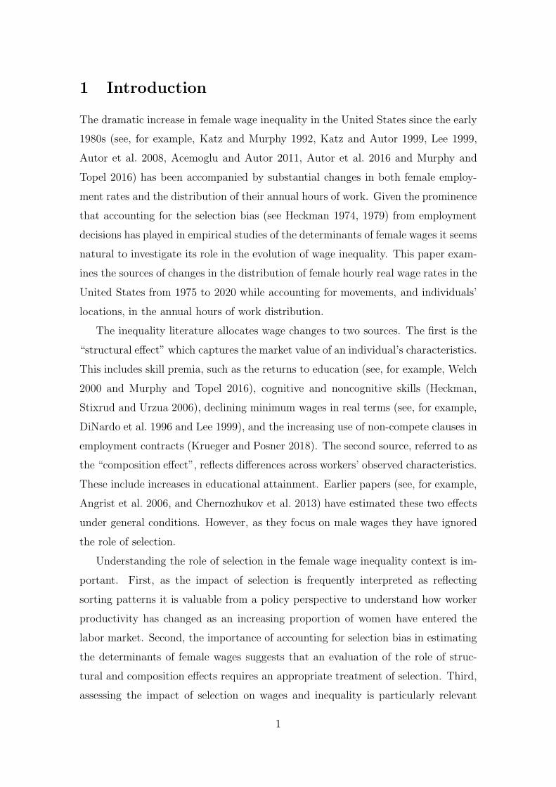
Figure 4 reveals that the wage levels of FTFY workers, defined as working 52

weeks per year for at least 40 hours, are somewhat higher than for all workers. Their

fraction increased from 50 to 71%. The difference in wages diminishes at higher

quantiles and, though not reported here, becomes negligible at D9. Contrasting

full-year (FY) and full-time (FT) wages against non-FY and non-FT wages provides

a similar finding. The differences at the bottom of the distribution in comparison to

the top, may reflect that the choice of working FT and/or FY should be incorporated

in the selection model. Moreover, as non-FTFY (or non-FT/non-FY) workers are

potentially more vulnerable to interruptions it seems inappropriate to exclude them

in an evaluation of wage inequality. The wage differences between these two working

8

1980 1990 2000 2010 202050

60

70

80

90

100

Year

Percentage

Employment rate

1980 1990 2000 2010 2020

35

40

45

50

YearHou

rs/w

eeks

Average hours/weeks

ASEC MORG Weeks, ASEC Hours, ASECHours, MORG

Figure 3: Employment rates and hours/weeks worked of employees.

categories might also reflect selection effects. The failure to include those who do not

work FTFY means that the selection effects in earlier studies may reflect movement

from the non-FTFY to FTFY, rather than from non-employment to FTFY.

3 Econometric analysis

3.1 Model with Censored Selection

We consider a version of the HSM where the censoring rule for the selection pro-

cess incorporates the information on annual hours worked rather than the binary

employment/non-employment decision. The model has the form:

Y = g(X,E), if D = 1, (1)

H = h(Z, V ), if D = 1, (2)

D = 1{h(Z, V ) > µ(Z)}, (3)

where Y is the logarithm of hourly wages, H is annual hours worked, D is a selection

or employment indicator equal to 1 if H and Y are observed or equivalently if H

9

1980 2000 20202

2.5

3

3.5

Year

Log

hou

rlywages

Median

1980 2000 2020

Year

Q1

1980 2000 2020

Year

Q3

Non-FTFY FTFY

Figure 4: Percentiles of real log hourly wages by full-time full-year (FTFY) employ-ment status

is not censored at µ(Z), X and Z are vectors of observable conditioning variables,

g, h and µ are unknown functions, and E and V are respectively a vector and a

scalar of potentially dependent unobservable variables with cumulative distribution

functions (CDFs) FE and FV . We assume that X is a, not necessarily strict, subset

of Z, i.e. X ⊆ Z.

We refer to equation (3) as the selection rule. It corresponds to censored selection

with an unobserved censoring point, that is we observe the censoring status, D, but

not the censoring point, µ(Z). Equations (2)–(3) can be considered a reduced-form

representation for hours worked. The model is a nonparametric and nonseparable

version of the Tobit type-3 model considered by FVV, extended to incorporate an

unknown censoring threshold which is a function of Z. This threshold is motivated

by fixed labor costs measured in terms of hours. Individuals only work if the desired

number of hours exceeds a minimum number given by µ(Z). Cogan (1981) shows

that fixed labor costs reduce the number of individuals working very few hours. We

allow the fixed labor costs to vary by individual and household characteristics.

Let ⊥⊥ denote stochastic independence. We assume:

Assumption 1 (Control Function) (E, V ) ⊥⊥ Z , V is a continuously distributed

random variable with strictly increasing CDF on the support of V , and v 7→ h(Z, v)

is strictly increasing a.s.

10

Without loss of generality, we can normalize V to be standard uniformly dis-

tributed. The potential dependence between E and V implies Z ′s independence of

E in the entire population does not exclude dependence in the selected population

with D = 1. FVV showed that Z is independent of E conditional on V and D = 1

when µ(Z) = µ. Let H∗ = h(Z, V ). Lemma 1 extends FVV’s result to our model.

Lemma 1 (Existence of Control Function) Under the model in (1)–(3) and

Assumption 1:

E ⊥⊥ Z | V,D = 1.

Moreover, V = FH∗ |Z(H |Z) for H∗ = h(Z, V ), and FH∗ |Z is identified by

FH∗ |Z(h | z) = 1− π(z)[1 − FH |Z,D(h | z, 1)],

where π(z) = P(D = 1 |Z = z) is the propensity score of selection.

The proof of the first statement follows from the same argument as in Lemma 1 of

FVV. Thus, conditioning on (Z, V ) makes D = 1 or h(Z, V ) > µ(Z) deterministic.

The assumption that Z is independent of (E, V ) then proves the result implying

that V is an appropriate control function.3 The result V = FH∗ |Z(H |Z) follows

directly from the assumption that h is strictly increasing in its second argument

and the normalization on the distribution of V . Identification of FH∗ |Z follows from

Buchinsky and Hahn (1998). In the Appendix, we propose an estimator of FH∗ |Z

based on distribution regression. This estimator is an alternative to the estimators

of Buchinsky and Hahn (1998) and Chernozhukov and Hong (2002), which are based

on quantile regression.

The decompositions presented below require a wage distribution which incorpo-

rates the value of V and a statement regarding the region in which it is identified.

To proceed, we denote the support of random variables and vectors by calligraphic

letters while lower case letters in parentheses indicate that the support is condi-

tional on a stochastic vector taking a particular value; e.g. Z(x) is the support of

Z |X = x. We define the Local Average Structural Function (LASF) and Local

3This result is closely related to that of Imbens and Newey (2009), who consider estimation andidentification of a nonseparable model with a single continuous endogenous explanatory variable.

11

Distribution Structural Function (LDSF) as:

µ(x, v) := E[g(x, E) | V = v], G(y, x, v) := P[g(x, E) ≤ y | V = v]. (4)

They represent the mean and distribution of Y if all individuals with control function

equal to v had observable characteristics equal to x. An argument similar to FVV

shows that:

µ(x, v) = E[Y | V = v,X = x,D = 1], G(y, x, v) = P[Y ≤ y | V = v,X = x,D = 1],

provided (x, v) ∈ XV∗, where:

XV∗ = {(x, v) ∈ X × V | ∃z ∈ Z(x) : h(z, v) > µ(z)}.

This set, referred to as the identification set by FVV, is identical to the support of

(X, V ) among the selected population. Lemma 1 implies that the LASF and LDSF

equal the mean and distribution of the observed Y conditional on (X, V ) and that it

is identified. This follows directly from (E, V ) ⊥⊥ Z and that (x, v) ∈ XV∗ implies

the ability to find a (z, v) combination for which h(z, v) > µ(z). We refer to FVV

for a discussion on how the size of the identified set depends on the availability of

exclusion restrictions on Z with respect to X .

There are different candidates for H in (2). As the ASEC provides both usual

hours worked per week and annual hours, calculated as the product of weeks worked

last year and the usual number of hours worked per week, we employ several al-

ternatives. Although the usual hours per week may be the variable in the ASEC

that is closest to the hours decision in labor supply models (Killingsworth, 1983),

it may also reflect whether the job has pre-set hours. Therefore, we employ the

annual measure which incorporates the weeks decision. As the extensive margin

may capture whether an individual has worked a positive number of hours in the

past year, we also investigate the use of the number of worked weeks. A theoretical

motivation for this measure follows from search models in which the offered wages

depend positively on the job offer arrival rate and negatively on the separation rate

(Burdett and Mortensen, 1998). As these rates also determine the number of weeks

12

worked, it implies a relationship between weeks worked and wages. The appropriate

censoring variable in the MORG is the number of hours worked in the reference

week. Note that this variable solves some of the problems mentioned above.

3.2 Counterfactual distributions

We consider counterfactual CDFs constructed by integrating the LDSF with respect

to different joint distributions of the conditioning variables and control function.4

Counterfactual CDFs enable the construction of wage decompositions and facilitate

counterfactual analyses similar to those in DiNardo et al. (1996), Nopo (2008), Fortin

et al. (2011), and Chernozhukov et al. (2013). We focus on CDFs for the selected

population. To simplify notation, the superscript s denotes that we condition on

D = 1. The decompositions are based on the following representation of the CDF

of the observed Y :5

P[Y ≤ y |D = 1] =: GsY (y) =

∫G(y, x, v) dF s

Z,V (z, v),

where:

F sZ,V (z, v) =

1{h(z, v) > µ(z)}FZ,V (z, v)∫1{h(z, v) > µ(z)} dFZ,V (z, v)

,

denotes the joint CDF of (Z, V ) in the selected population and FZ,V denotes the

joint CDF of Z and V in the entire population.

The counterfactual CDFs are constructed by combining the CDFs G and FZ,V

with the selection rule (3) for different groups, each group corresponding to a differ-

ent time period or a subpopulation defined by certain characteristics. Specifically,

let Gt be the LDSF in group t, FZk,Vkbe the joint CDF of Z and V in group k, and

let 1{hr(z, v) > µr(z)} be the selection rule in group r. The counterfactual CDF

of Y when G is as in group t, FZ,V is as in group k, and the selection rule is as in

group r is defined as:

GsY〈t,k,r〉

(y) =

∫Gt(y, x, v) 1{hr(z, v) > µr(z)} dFZk,Vk

(z, v)∫1{hr(z, v) > µr(z)} dFZk,Vk

(z, v), (5)

4Counterfactual means can be constructed similarly using the LASF in place of the LDSF; seeSection 3.5.

5 We refer to FVV for details.

13

provided that the integrals are well-defined. Since the mapping v 7→ h(z, v) is strictly

monotonic, the condition hr(z, v) > µr(z) in (5) is equivalent to the condition:

v > FH∗r |Z(µr(z) | z) = 1− πr(z), (6)

where FH∗r |Z(µr(z) | z) is the probability of working less hours than the censoring

point conditional on Z = z in group r and πr(z) is the propensity of working in that

group. Given GsY〈t,k,r〉

(y), the corresponding counterfactual quantile function (QF)

is:

qsY〈t,k,r〉(τ) = inf{y ∈ R : Gs

Y〈t,k,r〉(y) ≥ τ}, 0 ≤ τ ≤ 1. (7)

Under these definitions the observed CDF and QF of Y for the selected population

in group t are GsY〈t,t,t〉

and qsY〈t,t,t〉respectively.

Nonparametric identification of (5) and (7) depends on whether the integrals in

(5) are well defined. They are when two conditions are met. First, if Zk ⊆ Zr, then

πr is identified over all z combinations in the integral. Second, when (XVk∩XV∗r) ⊆

XV t, then the LDSF is identified for all combinations of z on which we integrate.

Here, XV∗r denotes the support of (X, V ) for the selected population in group r.

The identification conditions simplify when we consider two years for q, r, and t,

such as 0 and 1, which is relevant for the decompositions. For example, we need

XV1 ∩ XV∗0 ⊆ XV∗

1 and Z1 ⊆ Z0 to identify G〈1,1,0〉 and XV∗0 ⊆ XV∗

1 to identify

G〈1,0,0〉. A sufficient condition for XV1 ∩ XV∗0 ⊆ XV∗

1 and XV∗0 ⊆ XV∗

1 is that the

employment rates in year 0, conditional on X , are lower than those in year 1.

Using (7), we decompose the difference in the observed QF of Y for the selected

population between any two groups, say group 1 and group 0, as:6

qsY〈1,1,1〉− qsY〈0,0,0〉

= [qsY〈1,1,1〉− qsY〈1,1,0〉

]︸ ︷︷ ︸

[1]

+ [qsY〈1,1,0〉− qsY〈1,0,0〉

]︸ ︷︷ ︸

[2]

+ [qsY〈1,0,0〉− qsY〈0,0,0〉

]︸ ︷︷ ︸

[3]

, (8)

where [1] is a selection effect that captures changes in the selection rule given the

joint distribution of Z and V , [2] is a composition effect that reflects changes in

the joint distribution of Z and V , and [3] is a structural effect that reflects changes

6Note that alternative orders are possible. We investigated the impact of changes in the orderon our empirical results and these were minor. Details are available upon request.

14

in the conditional distribution of Y given Z and V . These effects are relative to

the base year. We stress that this definition of the selection effect differs from the

standard definition. This is discussed in Section 3.5.

3.3 Double selection mechanism

The model can be extended to a multiple censored selection mechanism operating

through both weeks and hours. The model has the form:

Y = g(X,E), if h(Z, VH) > µH(Z) and w(Z, VW ) > µW (Z), (9)

H = h(Z, VH), if h(Z, VH) > µH(Z), (10)

W = w(Z, VW ), if w(Z, VW ) > µW (Z), (11)

where the unobserved thresholds µH(Z) and µW (Z) are functions of the individual’s

characteristics.7 The distributions of H∗ := h(Z, VH) and W ∗ := w(Z, VW ) condi-

tional on Z, denoted VH and VW , respectively, are each required as control functions.

The analysis of this model is similar to that above. However, it is necessary to em-

ploy both control functions to, for example, calculate the LDSF, i.e.

G(y, x, vH, vW ) = P(g(x, E) ≤ y | VH = vH , VW = vW ).

The identification conditions change to accommodate that the support condition

is defined over two control functions. Using the same notation as Section 3.2,

the support requirements for the counterfactuals are ZVHVW,k ⊆ ZVHVW,r and

(XVHVW,k ∩ XVHV∗W,r) ⊆ XVHVW,t. We acknowledge that there are circumstances

under which this model will collapse to the single censoring mechanism case. How-

ever, as these are somewhat obvious we do not detail them here.

3.4 Model with ordered selection

The models above employ control functions which assume that the selection vari-

able is continuous. However, both the numbers of weeks and hours worked feature

7A further complication could be introduced by assuming that either the equation (10) or (11)is the sole source of selection.

15

bunching at specific values (e.g. 40 hours and 52 weeks). The following model with

ordered selection incorporates bunching:

Y = g(X,E) if H ≥ 1,

H =

0 if V ≤ µ0(Z),

1 if µ0(Z) < V ≤ µ1(Z),

...

K if V > µK−1(Z),

where the variables have similar interpretations as above. The main difference be-

tween this model and those above is that it allows a discrete distribution of H at the

expense of requiring separability in the selection process. We assume Z ⊥⊥ (E, V )

and V follows a standard uniform distribution. This model is related to the or-

dered choice model of Heckman and Vytlacil (2007, p. 4980), but unlike their model

g(X,E) does not depend on H . It can also be interpreted as an extension of Newey

(2007) to multiple ordered outcomes.

We define the identification set as:

XPK := {(x, p) ∈ X × [0, 1) | ∃(h, z) ∈ HZ(x) : µh′(z) = p, h′ ≤ h, h > 0}.

This set collects (x, p) combinations in the selected sample (i.e. H = h > 0) for

which there is a (h, z) combination inHZ(x) such that µh′(Z) = p for the propensity

score of a value of H smaller or equal than the observed value h. For example, if

H = 3, this restriction is satisfied when µh′(z) = p, for some h′ ∈ {0, 1, 2, 3}. We

define the LDSF as in (4). We prove the following lemma in the Appendix.

Lemma 2 Suppose that (x, p) ∈ XPK and Z(x, h) = Z(x) for all h > 0. Then,

1

1− p

∫ 1

p

G(y, x, v)dv = P(Y ≤ y |X = x,H > h, µh(Z) = p),

and the probability in the RHS is identified.

Lemma 2 implies (x, p) ∈ XPK is also a sufficient condition for identification as

16

(see also Heckman and Vytlacil, 2007):

G(y, x, p) = −∂

∂p

∫ 1

p

G(y, x, v)dv =∂

∂p{(1− p)P(Y ≤ y |X = x,H > h, µh(Z) = p)} .

We need additional assumptions to obtain counterfactual distributions. In the

models with continuous censoring we hold the value of the control function constant

and change the lowest value at which the individual is participating (see (6)). We

cannot follow the same strategy here as V is not point identified. However, from

the values of H and Z we know that the value of V is between µH−1(Z) and µH(Z).

This implies that individuals with H = 1 have the lowest values of V . Therefore, if

we increase µ0(Z), while leaving V unchanged, some individuals with H = 1 would

no longer participate although we do not know who. Hence, we integrate over the

distribution of V and change the range of integration accordingly. We show in the

appendix that:

GsY (y) =

∑K

h=1

∫Z

∫ µh(z)

µh−1(z)G(y, x, v)dvdFZ(z)∫

Z(1− µ0(z))dFZ(z)

, (12)

where µK(z) := 1 for any z. This equation is comparable to equation (7.2) of

Heckman and Vytlacil, 2007). Based on (12), the counterfactual distribution when

G is as in group t, FZ is as in group k, and the selection rule is as in group r is:

GsY〈t,k,r〉

(y) =

∫Zk

∫ µk1(z)

µr0(z)

Gt(y, x, v)dvdFZk(z)∫Zk(1− µr

0(z))dFZk(z)+

∑K

h=2

∫Zk

∫ µkh(z)

µkh−1

(z)Gt(y, x, v)dvdFZk(z)

∫Zk(1− µr

0(z))dFZk(z).

(13)

The decompositions are identical to (8). The identification restrictions are related

to the integrals in (13). The integral in the numerator of the second line of (13) can

be written as

∫

Zk

[∫ 1

µkh−1

(z)

Gt(y, x, v)dv −

∫ 1

µkh(z)

Gt(y, x, v)dv

]dFZk(z).

For both of these terms to be identified for any h, we need that XPkK ⊆ XP t

K . For

17

the identification of the integral in the numerator of the first line of (13), a similar

argument gives (XPrK ∩ XPk

K) ⊆ XP tK . We also need that Zk ⊆ Zr otherwise

µr0(z) is not identified. The identification restrictions imply that, for example, to

identify GsY〈1,1,0〉

, one needs that XP0K ⊆ XP1

K and Z1 ⊆ Z0. The interpretation of

these restrictions not only depends on the employment rates between year 0 and 1

but also on whether the propensity scores in year 1 overlap those of year 0.

Despite these requirements, there is a benefit of using an ordered rather than

dichotomous selection rule. In the latter case, the restriction for GsY〈1,1,0〉

would have

been that the support of the propensity scores of employment for year 1, µ10(Z),

should overlap with those of year 0, µ00(Z). For ordered selection it is only necessary

that one of the propensity scores in year 1, i.e. µ1h(Z), h = 1, . . . , K, overlaps with

the propensity score of employment for year 0, i.e. µ00(Z).

3.5 Comparison with the Heckman selection model

The decomposition (8) yields different effects to those derived by MR for a para-

metric version of the HSM. The MR selection effect excludes one component that

we attribute to the selection effect and includes another that we assign to the com-

position effect. Two other components are sorting effects that cannot be separately

identified from the structural effect in nonseparable models. A common measure of

a selection effect is the difference between the average wage for the selected pop-

ulation and that for the entire population. The change in the selection effect is

how this difference varies over time. We define the change in the selection effect as

the difference between the average wage in the selected population with that which

would result under a more restrictive selection rule.

To illustrate the difference with MR, suppose that the population model in period

t is the following parametric version of the HSM:

Yt = α′tXt + Et, if Ht > 0, (14)

Ht = max{γ′tZt + Vt, 0}, (15)

where the first element of Xt is the constant term, and Et and Vt are distributed

independently of (Xt, Zt) as bivariate normal with zero means, variances σ2Et

and

18

σ2Vt, and correlation coefficient ρt.

8 The counterfactual mean of Y for the selected

population when the LASF is as in group t, FZ,V is as in group k, and the selection

rule is as in group r, is:

µsY〈t,k,r〉

=

∫µt(x, v) 1{v > Φ(−γ′

rz)}dFZk,Vk(z, v)∫

1{v > Φ(−γ′rz)} dFZk,Vk

(z, v), (16)

where:

µt(x, v) = α′tx+ ρtσEt

Φ−1(v),

denotes the LASF in group t. The observed mean of Yt in the selected population,

integrating over Zt, is:

µsY〈t,t,t〉

= α′t E[Xt |Ht > 0] + ρtσEt

E[λ(γ′tZt/σVt

) |Ht > 0],

where λ denotes the inverse Mills ratio. We decompose the difference µsY〈1,1,1〉

−µsY〈0,0,0〉

between two time periods, t = 0 and t = 1, into selection, composition and structural

effects.

MR define the selection effect as:

ρ1σE1E[λ(γ′

1Z1/σV1) |H1 > 0]− ρ0σE0

E[λ(γ′0Z0/σV0

) |H0 > 0]. (17)

This comprises the following four elements:

ρ1σE1

∫[λ(γ′

1z/σV1)Φ1(γ

′1z/σV1

)− λ(γ′0z/σV0

)Φ1(γ′0z/σV0

)] dFZ1(z)+

+ ρ1σE1

[∫λ(γ′

0z/σV0)Φ1(γ

′0z/σV0

) dFZ1(z)−

∫λ(γ′

0z/σV0)Φ0(γ

′0z/σV0

) dFZ0(z)

]+

+ ρ1 (σE1− σE0

)E [λ (γ′0Z1/σV0

) |H0 > 0]+

+ σE0(ρ1 − ρ0)E [λ (γ′

0Z1/σV0) |H0 > 0] , (18)

where Φk(γ′rz/σVr

) = Φ(γ′rz/σVr

)/∫Φ(γ′

rz/σVr) dFZk

(z) is the counterfactual prob-

ability of selection in group k when the selection rule is as in group r and Φ denotes

the standard normal CDF. The first two elements in (18) capture the effect of

8We present the selection rule in this censored form in order to employ our approach althoughour discussion of the HSM which follows is based on the binary rule that only 1(Ht > 0) is observed.

19

changes over time in the observable characteristics of the selected population. The

first results from applying the selection rule from period 1 to period 0 holding the

composition of period 1 fixed. The second captures changes in the distribution of

characteristics from period 1 to period 0. The third element captures the effect of

changes over time in the composition of the selected population in terms of unob-

servables through the variance in wages. The fourth element is a sorting effect that

captures changes over time in the composition of the selected population in terms

of unobservables through the correlation coefficient.9 In our view the first element

belongs to the selection effect while the second element belongs to the composition

effect as it is driven by changes over time in the distribution of Z. It is also not clear

why the change in the variance of wages should be interpreted as a selection effect

as it captures factors potentially unrelated to selection. As the final element reflects

changes how unobservables are valued it is arguably a component of the selection

effect. However, it could be assigned the interpretation of a structural effect as it

captures the market value of unobserved characteristics. We agree with the MR

interpretation that the sign of ρt captures the nature of sorting.

We now present the selection, composition and structural effects for our decom-

position. Plugging the expression for µt(x, v) into (16) gives, after some straightfor-

ward calculations:

µsY〈t,k,r〉

=

∫[α′

tx+ ρtσEtλ(γ′

rz/σVr)] Φk(γ

′rz/σVr

) dFZk(z).

Our selection effect is:

µsY〈1,1,1〉

− µsY〈1,1,0〉

= α′1

∫x [Φ1(γ

′1z/σV1

)− Φ1(γ′0z/σV0

)] dFZ1(z)+

+ ρ1σE1

∫[λ(γ′

1z/σV1)Φ1(γ

′1z/σV1

)− λ(γ′0z/σV0

)Φ1(γ′0z/σV0

)] dFZ1(z). (19)

The first element on the right-hand-side of (19) is the effect on the average wage

from changes in the distribution of observable characteristics of the selected pop-

ulation, holding the population distribution constant, resulting from applying the

selection equation from period 0 to period 1. It is positive if those entering the

9 MR make the strong assumption that the distribution of the covariates does not change overtime, i.e., FZ0

= FZ1, so the second component drops out.

20

selected population have characteristics associated with higher wages. This element

is missing in the selection effect in (18). The second element is the corresponding

effect for the unobservable characteristics and corresponds to the first in (18).

Our composition effect is:

µsY〈1,1,0〉

− µsY〈1,0,0〉

= α′1

[∫xΦ1(γ

′0z/σV0

) dFZ1(z)−

∫xΦ0(γ

′0z/σV0

) dFZ0(z)

]+

+ρ1σE1

[∫λ(γ′

0z/σV0)Φ1(γ

′0z/σV0

) dFZ1(z)−

∫λ(γ′

0z/σV0)Φ0(γ

′0z/σV0

) dFZ0(z)

].

(20)

The first element on the right-hand side of (20) is the change in the average wage

resulting directly from changes over time in the distribution of the observable char-

acteristics while the second element is the same as the second term in (18).

Finally, our structural effect is:

µsY〈1,0,0〉

−µsY〈0,0,0〉

= (α1 − α0)′E [X0|H0 > 0]+(ρ1σE1

− ρ0σE0)E [λ (γ′

0Z0/σV0)|H0 > 0] .

(21)

The first element on the right-hand side of (21) reflects the impact of changes over

time in the returns to observable characteristics while the second captures the type

and degree of sorting and is the same as the sum of the third and fourth elements in

(18). As the expectation involving the inverse Mills ratio is positive, its contribution

is positive when ρ1σE1> ρ0σE0

.

Finally, consider a simple example illustrating that the two elements of the struc-

tural effect cannot generally be identified in nonseparable models.10 Consider a

multiplicative version of the parametric HSM obtained by replacing (14) with:

Yt = α′tXtEt, if Ht > 0,

and weaken the parametric assumption on the joint distribution of Et and Vt by only

requiring that Vt ∼ N(0, 1) and E[Et |Zt, Ht > 0] = ρtλ(γ′tZt). αt and ρt cannot be

10Chernozhukov et al. (2019) separate the structural effect from the sorting effect using anexclusion restriction in the copula for the unobservables of the employment and wage equation.They provide a wage decomposition with 4 components: structural, composition, selection andsorting. Compared to our decomposition, the composition and selection effects are the same, butour structural effect corresponds to the sum of their structural and sorting effects.

21

separately identified from the moment condition:

E[Yt |Zt, Ht > 0] = α′tXt ρtλ(γ

′tZt).

4 Empirical results

4.1 Hours equation

We start by describing the variables included in Z using the ASEC. Following MR,

we include six indicator variables for the highest educational attainment reported.

Namely, (i) 0-8 years of completed schooling, (ii) high school dropouts, (iii) high

school graduates or 12 years of schooling, (iv) some college, (v) college, and (vi)

advanced degree. We include a quartic polynomial in potential experience and

interact this with the education levels.11 We use 5 indicator variables for marital

status: (1) married, (2) separated, (3) divorced, (4) widowed, and (5) never married.

We include indicator variables for Black and Hispanic and four indicator variables

for regions: northeast, midwest, south and west. Finally, we use linear terms for

the number of children aged less than 5 years interacted with the indicator variables

for marital status. For the MORG we use 5 levels of education as the two lower

categories in the ASEC are merged. The variables Black, Hispanic, experience and

region are the same. Only one indicator for marital status is used (married or not)

and we employ household size, and its interaction with marital status, as the only

household characteristic.

With the exception of the household size and composition variables, all of the

conditioning variables appear as both determinants of annual hours and hourly

wages. While one might argue that household size and composition may affect hourly

wage rates, we regard these exclusion restrictions as reasonable and note that similar

restrictions have been previously employed (see, for example, MR). However, given

their potentially contentious use we explore the impact of not using them below.

The assumption that annual hours of work do not affect the hourly wage rate means

that the variation in hours across individuals is a source of identification.

Although our primary focus is the wage decomposition, we highlight the ma-

11We employ the methodology described in MR for education and potential experience.

22

1980 2000 20200

5 · 10−2

0.1

0.15

0.2

Year

Average

derivative

010002000

Figure 5: Average derivative of the exclusion restriction at different levels of hours.

jor features of the hours equation estimates. The hours equation is estimated by

distribution regression and we report the marginal impact of being below a certain

point in the annual hours distribution. We do this for education level, race, marital

status and for one of the exclusion restrictions (having a child below the age of 5).

We only report the result of the latter here; see Figure 5. The selected points in

the hours distribution are 0, 1000 and 2000. We find that many of the individual

characteristics have an impact on the level of annual hours worked. This is not

particularly surprising given the large literature on labor supply documenting the

roles of education and marital status on labor market participation. Perhaps what

is more surprising is that the magnitude of the impact of these variables does not

appear to change substantially over the sample period in either the ASEC or MORG

data. The exception is with respect to the exclusion restrictions which became less

important over time. This is consistent with Card and Hyslop (2021). Note that

the level of education has drastically increased over the sample period and this has

had a substantial impact on the hours distribution.

We also estimated models for annual weeks of work using distribution regression

and ordered models for annual weeks and annual hours using the ASEC. The flavor

of the results are very similar to those for the annual hours equations. The individual

variables which also appear in the wage equations are statistically significant and

their impact does not appear to change a great deal over the sample period. The

variables employed as exclusion restrictions have a statistically significant impact

23

on the level of reported work.

4.2 Decompositions

The wage equations are estimated for each year by distribution regression over the

subsample with positive hourly wages. The conditioning variables are those in the

hours equation with the exception of the household size and composition variables.

We also include the appropriate control function, its square, and interactions be-

tween the other conditioning variables and the control function. The decompositions

require a base year. The steadily increasing female participation rate suggests that

1975 is a reasonable choice as it has the lowest level of participation. It is reasonable

to assume that those with a certain combination of x and v working in 1975 also

have a positive probability of working in other years as required by the identification

conditions. We present results for the censoring mechanism being either the number

of annual hours or the number of annual weeks for the ASEC. These are shown in

Figures 6 and 7 respectively. The results for the MORG, using numbers of hours

in reference week as the censoring mechanism, are in Figure 8. Before presenting

the decompositions we highlight that they reflect the change in the contributions of

each component over time. For example, if the structural effects are zero this should

be interpreted as the contribution of the structural effects not changing, not that

there are no structural effects.

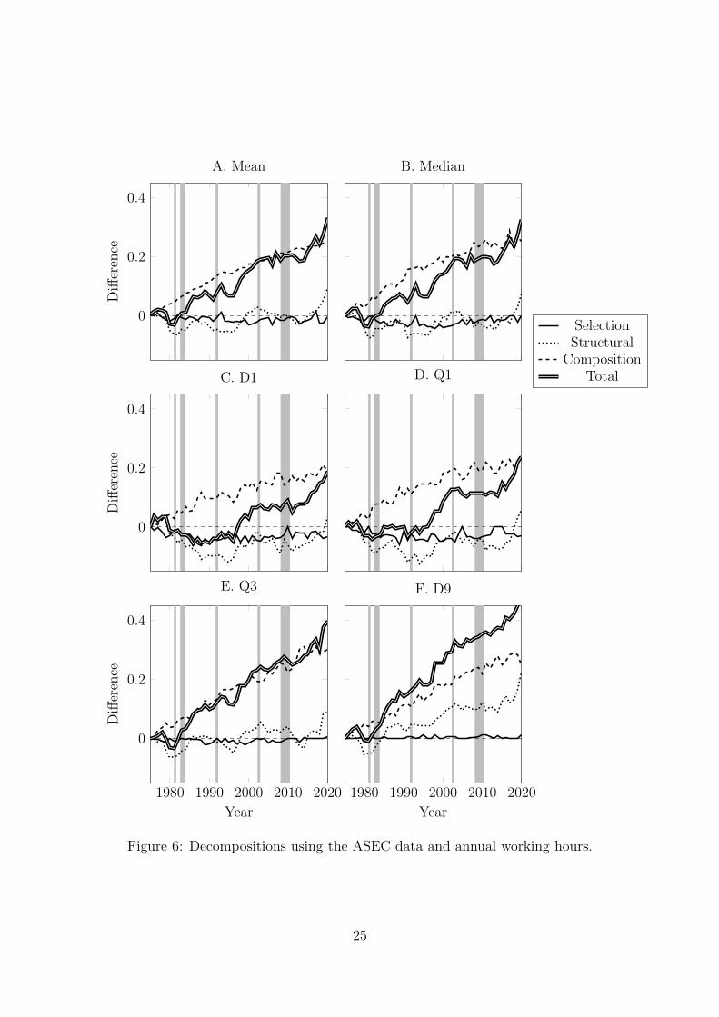
We start with annual hours as the censoring mechanism and Figure 6A presents

the decomposition for the mean, which increases by 25% over our sample period.

The total effect is driven by the composition effect although in several instances

the structural effect is contributing. It is generally negative and small relative to

the composition effect. The contribution of the selection component is negative and

small. A negative selection component implies that females are positively selected

into employment and those who entered employment between 1975 and 2020 were

less productive than those already employed.

Figures 6B– 6F present the decompositions for the 10th, 25th, 50th, 75th and

90th percentiles. A number of important conclusions can be drawn. The large in-

creases at each quantile are driven by the large changes in the composition effects.

This reflects the increasing education levels of the female workforce. The large in-

24

0

0.2

0.4

Difference

A. Mean B. Median

0

0.2

0.4

Difference

C. D1 D. Q1

1980 1990 2000 2010 2020

0

0.2

0.4

Year

Difference

E. Q3

1980 1990 2000 2010 2020

Year

F. D9

SelectionStructural

CompositionTotal

Figure 6: Decompositions using the ASEC data and annual working hours.

25

0

0.2

0.4

Difference

A. Mean B. Median

0

0.2

0.4

Difference

C. D1 D. Q1

1980 1990 2000 2010 2020

0

0.2

0.4

Year

Difference

E. Q3

1980 1990 2000 2010 2020

Year

F. D9

SelectionStructural

CompositionTotal

Figure 7: Decompositions using the ASEC data and annual working weeks.

26

−0.2

0

0.2

0.4

Difference

A. Mean B. Median

−0.2

0

0.2

0.4

Difference

C. D1 D. Q1

1980 1990 2000 2010−0.2

0

0.2

0.4

Year

Difference

E. Q3

1980 1990 2000 2010

Year

F. D9

SelectionStructural

CompositionTotal

Figure 8: Decompositions using the MORG data and annual working hours.

27

1980 1990 2000 2010 2020

0

0.5

1

Year

Average

derivative

A. D1

D1Q1

MedianQ3D9

Mean

Figure 9: Average derivatives at different quantiles

creases from the composition effects at each quantile are somewhat offset by the

structural effects at lower quantiles and there is only clear evidence of an econom-

ically important and positive structural effect at D9. At this quantile almost half

of the 44% increase in real wages experienced over the sample period is due to the

structural effect. At lower quantiles the structural effects are somewhat cyclical

while the sustained increase at D9 reflects the increasing skill premia.

Figures 6B– 6F reveal no indication of changes in the selection effects at Q3 and

D9. Individuals located here are likely to have had a relatively strong commitment

to employment in 1975 and there have been no substantial movements in their

hours distribution. Moreover, these individuals are less likely to incur periods of

unemployment. Lower down the wage distribution there is evidence of small negative

changes in selection during some years in our sample. At D1 and Q1 the selection

effects are negative and economically important. The confidence intervals for these

selection effects are presented in Figure 10. They indicate that for several time

periods selection effects are statistically significantly different from zero. At D1 the

total real wage increase is less than 10% for the majority of the sample period and

the negative selection effect is frequently of the order of around 3%.

We explore the form of sorting implied by these results. Given the non-separable

nature of the model, this is not straightforward although one indication of the sort-

ing pattern is how wages change at each quantile in response to a change in the

28

control function. This corresponds to the local average derivative function of FVV

evaluated at each quantile. This is somewhat comparable to the coefficient on the

selection term in the HSM. A positive average derivative at a specific quantile sug-

gests that the unobservables increasing hours are positively correlated with wages at

that quantile. The results are shown in Figure 9. At D1, Q1 and Q2 these estimated

derivatives are positive and large for the whole sample period. At Q3 the derivative

is positive for the vast majority of the sample period although there are instances

where it is close to zero or very slightly negative. At D9 it is negative but small

in magnitude. The results clearly support the existence of a positive relationship

between V and wages at the bottom of the distribution implying positive selection

which is more important in the lower half of the wage distribution. This is similar

to the findings of AB for female wages in the British labor market for 1978 to 2000.

Annual hours is an economically attractive censoring mechanism as it exploits

the variation in annual hours induced both by hours and by weeks. However, it

is possible that selection operates either through hours or weeks exclusively. We

first address this issue by replacing annual hours with annual weeks as the selection

mechanism. The results from these decompositions using the ASEC are in Figures

7A–7F. Their primary feature is their similarity to those for annual hours. This sug-

gests that the control function from the annual hours censoring mechanism is highly

correlated with that from annual weeks despite the differences in their respective

distributions.

Now consider the decompositions for the MORG recalling that wages are mea-

sured differently than in the ASEC and the hours measure is based on the survey

week. We implement our censored selection estimator using hours in the survey week

as the censoring mechanism noting that only a subset of the exclusion restrictions

used in the ASEC are available in the MORG. The results are shown in Figures

8A-8F. As the MORG covers a different sample period, the figures look slightly

different from those for the ASEC. Nevertheless, the findings regarding the role of

selection are almost identical. The similarity across figures is remarkable given the

differences in measurement, data and exclusion restrictions.

We acknowledge that although also employed by MR and MW, the use of house-

hold composition variables as exclusion restrictions is controversial. Accordingly,

29

−0.1

0

0.1

Selection

compon

ent

10th percentile 25th percentile

1980 1990 2000 2010 2020−0.1

0

0.1

Year

Selection

compon

ent

50th percentile

1980 1990 2000 2010 2020

Year

75th percentile

Figure 10: Selection components and associated 95% confidence intervals for femalesat various percentiles

30

we reproduced the decompositions from the censored selection mechanisms first ex-

cluding the household variables from both the hours and wage equations and then

including them in both equations. The model is now only identified by the varia-

tion in the number of hours worked. We do not find any remarkable changes from

either model, in comparison to the specification employed above, with respect to

the presence or magnitude of selection effects. The only notable difference is the

presence of occasionally larger negative selection effects at the bottom decile for the

specification which excludes the family composition variables from both equations.

4.3 Results of the double selection model

Our results from Section 4.2 seem robust to the use of either hours or weeks as

the selection variable in the censored selection model. Figures 11A–11C report

the decomposition for the double selection mechanism. There continues to be no

evidence of selection above the median so we report the decompositions for D1, Q1

and the median.

While there are some differences in these figures compared to those for selection

using only annual hours or annual weeks they are relatively small. These results

seem to suggest that the unobservables which increase participation on any margin,

such as usual weeks, usual hours, hours in survey week, are all highly correlated. To

pursue this possibility we estimate the average derivative with respect to each of the

control functions evaluated at the mean wage as this provides some insight into the

source of selection. The derivatives, reported in Figure E.1 in the appendix, indicate

that at the mean wage both sources of selection are important. The derivative for the

weeks’ control function is the bigger of the two and the effect is relatively constant

with the exception of a notable decrease at the time of the financial crisis. The

hours’ control function derivative is negative for the earliest years of the sample

before turning and remaining positive for the remaining years. Prior to the financial

crisis it increases in magnitude and for a very short period it is the larger of the

two. The high correlation between the two control functions makes it difficult to

interpret this figure but this evidence suggests that selection operates both through

the weeks and hours decisions and the effect of each is similar.

31

1980 2000 2020

0

0.2

0.4

Year

Difference

A. D1

1980 2000 2020

Year

B. Q1

1980 2000 2020

0

0.2

0.4

Year

Difference

C. Median

SelectionStructural

CompositionTotal

Figure 11: Decompositions using a double selection mechanism based on ASECdata.

32

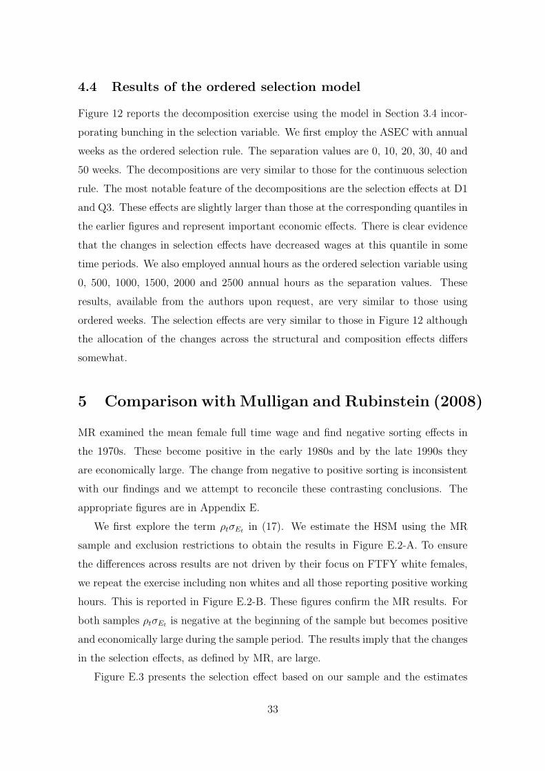
4.4 Results of the ordered selection model

Figure 12 reports the decomposition exercise using the model in Section 3.4 incor-

porating bunching in the selection variable. We first employ the ASEC with annual

weeks as the ordered selection rule. The separation values are 0, 10, 20, 30, 40 and

50 weeks. The decompositions are very similar to those for the continuous selection

rule. The most notable feature of the decompositions are the selection effects at D1

and Q3. These effects are slightly larger than those at the corresponding quantiles in

the earlier figures and represent important economic effects. There is clear evidence

that the changes in selection effects have decreased wages at this quantile in some

time periods. We also employed annual hours as the ordered selection variable using

0, 500, 1000, 1500, 2000 and 2500 annual hours as the separation values. These

results, available from the authors upon request, are very similar to those using

ordered weeks. The selection effects are very similar to those in Figure 12 although

the allocation of the changes across the structural and composition effects differs

somewhat.

5 Comparison with Mulligan and Rubinstein (2008)

MR examined the mean female full time wage and find negative sorting effects in

the 1970s. These become positive in the early 1980s and by the late 1990s they

are economically large. The change from negative to positive sorting is inconsistent

with our findings and we attempt to reconcile these contrasting conclusions. The

appropriate figures are in Appendix E.

We first explore the term ρtσEtin (17). We estimate the HSM using the MR

sample and exclusion restrictions to obtain the results in Figure E.2-A. To ensure

the differences across results are not driven by their focus on FTFY white females,

we repeat the exercise including non whites and all those reporting positive working

hours. This is reported in Figure E.2-B. These figures confirm the MR results. For

both samples ρtσEtis negative at the beginning of the sample but becomes positive

and economically large during the sample period. The results imply that the changes

in the selection effects, as defined by MR, are large.

Figure E.3 presents the selection effect based on our sample and the estimates

33

0

0.2

0.4

Difference

A. Mean B. Median

0

0.2

0.4

Difference

C. D1 D. Q1

1980 1990 2000 2010 2020

0

0.2

0.4

Year

Difference

E. Q3

1980 1990 2000 2010 2020

Year

F. D9

SelectionStructural

CompositionTotal

Figure 12: Decompositions using the ASEC data and annual working weeks usingour alternative model taking account of bunching.

34

from the HSM. The figure decomposes the total selection effect into the four compo-

nents shown in (18). It reveals that the movements in the selection effects are almost

entirely due to the change in ρt. The impact of the unobservables from the selection

equation on wages was initially negative but became positive and subsequently large.

Figure E.4 presents our selection, structural and composition effect based on (19)-

(21). We find that our selection effect is small and the majority of the wage change

reflects composition effects. However, Figure E.4 is similar to Figure 6-A obtained

via our approach. The reason for our smaller selection effect is clear from Figure

E.3. The figure reveals that the second component, which from (18) is included in

our selection effect, is small and similar in size to that of Figure 6-A and Figure

E.4. This suggests that the difference is partially due to the difference in definitions

recalling this reflects the inability to isolate the MR selection effects in nonseparable

models. We now examine whether components of the remaining difference reflect

the specific parametric form or the source of identification employed.

That ρt becomes large is not particularly controversial. However, its change of

sign has implications for the nature of sorting into the labor market. As ρt captures

the mapping from unobservables in the work equation to wages, we explore if our

approach uncovers the same pattern by evaluating once more the average derivative

as presented in Figure 9-A. While the derivative’s value at the mean fluctuates over

the sample period, it does not change sign and is always consistent with positive

sorting.

This contrasts with MR. The three obvious causes are the use of the normality

assumption in the HSM, the identifying power introduced through hours as a cen-

soring variable in the selection equation, and the nonseparable nature of our model.

To address these issues we first estimate the model using a parametric approach

which relies on normality but which exploits the variation in hours for identification

purposes. We employ the Vella (1993) procedure which estimates the hours equation

by Tobit and computes the generalized residual, defined for the H > 0 observations

as H −Z ′γ where γ is estimated by Tobit, to include as the correction for selection

in the wage equation. This assumes hours do not directly effect hourly wage rates.12

To more closely correspond to the HSM we divide the generalized residual by the

12Hirsch (2005) provides empirical evidence supporting this assumption.

35

estimated standard deviation of working hours, σVt. The only difference with the

HSM is the use of the Tobit generalized residual rather than the inverse Mills ratio.

We plot the corresponding coefficient on the Tobit generalized residual in Figure

9-B. The coefficient on the Tobit generalized residual also estimates ρtσEt.

Two striking features are revealed in Figure 9-B. First, under normality the es-

timates of ρtσEtand the coefficient on the generalized residual should be identical.

However, the estimates are very different and most importantly the coefficient es-

timate is always positive. As there is no reason that departures from normality

will bias the estimates of ρtσEtand the coefficient for the Tobit generalized residual

in the same manner one could interpret the difference in the estimates as evidence

of non-normality. However, recall that the Tobit generalized residual also exploits

variation in the hours variable for identification purposes and this could contribute

to the difference in the signs and the behavior of the two coefficients. Second, the

pattern of movement in the coefficient on the generalized residual is almost identi-

cal to the average derivative of our control function despite the drastically different

ways in which each is computed. The two procedures are very different but each

exploits the variation in hours as a means of identification.

While it appears that the use of the variation in hours as the source of identi-

fication is the cause of the differences with MR, it is possible that the departures

from normality may also be responsible. The final approach we explore is the use

of the propensity score as the control function noting we allow it to enter the wage

equation in a nonseparable manner (see, for example, Newey, 2007). The propen-

sity score employs the exclusion restrictions as the sole source of identification. We

estimated the model and computed the average derivative of wages with respect to

the propensity score. The results are presented in Figure 9-C. This derivative also

changes sign as we move through the sample period and shows behavior similar to

ρt. We conclude that the differences in terms of the relationship between Et and

Vt between our results and MR are due to the use of the variation in hours which

appear to identify a different pattern of sorting.

For reconciling the difference in the results associated with the two controls, it

is necessary to examine their sources of variation. For the subsample of workers,

the variation in their values of the inverse Mills ratio is due to the variation in

36

Z. In contrast, an individual’s value of the Tobit generalized residual also exploits

the value of H. Consider a case where ρt is positive and there are two working

individuals with identical Z but one receives a much larger positive value of Vt.

This produces a relatively larger positive value of Et and that individual will have

relatively higher hours and wages. In this setting the value of the inverse Mills ratio

for both individuals will be the same while the Tobit generalized residual of the

individual with the higher value of H will be greater than the other. This suggests

that the Tobit generalized residual is capturing information regarding “sorting” into

hours which is ignored by the inverse Mills ratio. Moreover, the inverse mills ratio,

unlike the Tobit generalized residual, is unable to explain the variation in wages

across these two individuals.

It is important to explore why ρt might change sign for the models identified

solely by exclusion restrictions. A negative ρt implies that the working individuals

with the lowest probabilities of participation should have the lowest observed wages

among individuals with the same observed characteristics relevant for the wages,

X . The reverse is true for a positive ρt. We explore this by estimating a wage

regression identical to the second stage of MR while replacing the inverse Mills ratio

by a dummy variable for a child below the age of 5 years. The impact of having

a “young child” was negative until 1982 at which time it turned, and remained,

positive. This corresponded to a period, also reported by Card and Hyslop (2021),

in which the magnitude of the negative impact of a “young child” on the employment

decision decreased. While we acknowledge the presence of other ongoing factors this

change in the impact of “young child” could generate a change in the sign of ρt. For

example, in the absence of other influences, the large positive influence of “young

child” on the value of the inverse Mills ratio combined with negative correlation

between “young child” and wages would produce a negative value of ρt. In contrast

a decreasing effect of “young child” on participation would produce a smaller value

for the inverse Mills ratio and that, combined with the positive correlation between

“young child” and wages, would produce a positive ρt.

We highlight that we consider the above discussion as suggestive rather than

conclusive. Our objective is to consider the possible causes of the differences in the

results from the use of the two control functions. The evidence suggests that part

37

1980 1990 2000 2010 2020−0.1

0

0.1

0.2

0.3

0.4

Year

Difference

Interquartile ratio

1980 1990 2000 2010 2020

Year

Interdecile ratio

SelectionStructural

CompositionTotal

Figure 13: Decompositions of the interquartile and interdecile ratio using the ASEC.

of the difference is due to the use of variation in hours as a source of identification

for ρt. However, it is clear that the effect of the exclusion variables on the hours and

work decisions is also an important factor in identifying ρt, and this has changed over

time. Related to this last issue is the validity of the exclusion restrictions employed

and how this validity has changed over the sample period. While the use of either of

the control functions should produce consistent estimates of the sorting parameters

when the model is correctly specified, the impact under misspecification is unclear.

6 Wage Inequality

We noted above that despite the large literatures on the impact of selection on

females’ wages and the increase in female wage inequality, there are few papers

which focus on both issues. The important exceptions are AB, MW and Blau et

al. (2021), which evaluate the impact of selection by contrasting changes in the

observed levels of wage inequality with the counterfactual levels associated with the

total population working. The latter corresponds to a participation rate of 100%.

We investigate the impact of selection by evaluating changes in the distributions,

and also inequality, by holding the selection rule constant across time. While both

approaches have merit we prefer ours as participation rates do not approach 100%

38

1980 1990 2000 2010−0.1

0

0.1

0.2

0.3

0.4

Year

Difference

Interquartile ratio

1980 1990 2000 2010

Year

Interdecile ratio

SelectionStructural

CompositionTotal

Figure 14: Decompositions of the interquartile and interdecile ratio using theMORG.

in the sample period.13

We provide the decompositions of changes in inequality using the annual hours

as the censored selection variable for the ASEC data, hours in the survey week for

the MORG and annual weeks as the ordered selection variable for the ASEC. For

each of these models and selection rules we decompose the interquartile and inter-

decile ratios. Those for annual hours using the ASEC are reported in Figure 13 and

those for the MORG in Figure 14. The interquartile ratio is driven by each of the

components. Neither the composition or structural effect dominates throughout the

sample period. The selection effect contributes throughout the period and clearly

increases inequality. The interdecile ratio is driven primarily by the structural ef-

fect especially during the drastic increase at the beginning of the sample period.

The selection effect is clearly important and frequently more important than the

composition effect. For the MORG the conclusions regarding the structural and

composition effects are similar to those for ASEC while the selection effects are

slightly smaller. This reflects the smaller selection effects at lower quantiles in the

wage decompositions (as presented in Figures 6 and 8). The evidence for both data

sets support that selection has a modest but important impact on wage inequality

that varies in magnitude over the sample period. As the wage decompositions based

13Chernozhukov et al. (2019) considered both approaches.

39

on the ordered selection rule suggested selection was more important than in the

censored selection models (see Figure 12) we examine now whether this carries over

to the inequality decompositions. We do not report the result but note that the

evidence is similar to that for the censored selection rule.

Our results indicate that as an increasing number of females have entered the la-

bor market they have reduced wages at the lower parts of the wage distribution while

having no impact on wages above Q2. This increases measures of inequality based

on ratios involving lower and upper quantiles. Potentially, there are two reasons why

selection increases inequality based on whether either the observed or unobserved

characteristics of those participating has changed over time. However, an exami-

nation of education levels, for example, suggests that observed characteristics have

played a minor role. In particular, we find that those with education higher than

high school degrees were more likely to participate over the whole sample period and

that this did not change over time. This suggests that our results reflect changing

unobserved characteristics. The selection effect captures the difference between the

observed wage distribution and the counterfactual in which women participated as

in 1975. Our decomposition method presented in (5) imposes that this difference

captures the exit of females with lower levels of the control function. Figure E.5,

reveals a strong and positive relationship between wages and the control function

suggesting that selection effects reflect that women entering the labor market were

less productive than observationally identical women participating in 1975.

Our evidence of positive sample selection over the whole period implies that the

decision to work is largely based on economic motivations. However, as employment

rates have increased this has seen a reduction in sorting on economic grounds. This

is consistent with the explanation provided by AB for the U.K. labor market. This

is also consistent with the results above that the conventional household background

family characteristics have become less important in explaining participation and

hours worked. The reduction in positive sorting describes the changes in the hours

distribution from the mid 1980s to the end of the 1990s. Blau et al. (2021) argue

that the booming economy and welfare reform may have played an important role

in the 1990s. Our collective evidence suggests that post 2000 there was an increase

in positive selection. This supports the evidence in Blau et al. (2021). Towards the

40

end of the sample period it appears that the impact of selection on inequality and,

more generally, wages has returned to 1975 levels.

7 Conclusions

This paper documents the changes in female real wages over the period 1975 to 2020.

We decompose these changes into structural, composition and selection components

by estimating a nonseparable model with selection. Female wage growth at lower

quantiles is modest although the median wage has grown steadily. The increases at

the upper quantiles for females are substantial and reflect increasing skill premia.

These changes have resulted in a substantial increase in female wage inequality. As

our sample period is associated with large changes in the participation rates and

the hours of work of females we explore the role of changes in “selection” in wage

movements. We find that the impact of these changes is to decrease the wage growth

of those at the lower quantiles with very little evidence of selection effects at other

locations in the female wage distribution. The selection effects appear to increase

wage inequality for the period 1975 to 2000 and this reflects a reduction in the level

of positive sorting. However, post 2000 there appears to be an increase in positive

sorting and the selection effects on wages and inequality appear to return to their

1975 levels by the end of our sample.

References

Acemoglu D., and D. Autor (2011), “Skills, tasks and technology: Implica-

tions for employment and earnings.” In D. Card and O. Ashenfelter (eds.),

Handbook of Labor Economics, Vol. 4B: 1043–1171. Amsterdam: Elsevier Sci-

ence, North-Holland.

Angrist J., Chernozhukov V., and I. Fernandez-Val (2006), “Quantile

regression under misspecification, with an application to the U.S. wage struc-

ture.” Econometrica, 74: 539–563.

Arellano M., and S. Bonhomme S. (2017), “Quantile selection models with

an application to understanding changes in wage inequality.” Econometrica,

41

85: 1–28.

Autor D. H., Katz L. F., and M. Kearney (2008), “Trends in U.S. wage

inequality: Revising the revisionists.” Review of Economics and Statistics, 90:

300–323.

Autor D. H., Manning A., and C. Smith (2016), “The contribution of the

minimum wage to US wage inequality over three decades: A reassessment.”

American Economic Journal: Applied Economics, 8: 58–99.

Blau, F.D., L.M. Kahn, N. Boboshko and M.L. Comey (2021), “The im-

pact of selection into the labor force on the gender wage gap.”, working paper,

Cornell University.

Beaudry P., Sand B. M., and D. Green (2016). “The great reversal in

the demand for skill and cognitive tasks.” Journal of Labor Economics, 34:

S199–247.

Bollinger C. R., Hirsch B. T., Hokayem C. M., and J. Ziliak (2019),

“Trouble in the tails? What we know about earnings nonresponse thirty years

after Lillard, Smith, and Welch.” Journal of Political Economy, 127: 2143–

2185.

Borjas G. (1980), “The relationship between wages and weekly hours of work:

The role of division bias.” Journal of Human Resources, 15: 409–423.

Buchinsky, M. and J. Hahn (1995), “Quantile regression model with unknown

censoring point.”working paper, Yale University, New Haven.

Buchinsky, M. and J. Hahn (1998), “An alternative estimator for the censored

quantile regression model.” Econometrica, 66: 653–71.

Burdett, K. and D.T. Mortensen (1998), “Wage differentials, employer size

and unemployment”, International Economic Review, 39: 257–73.

Card D., and D. Hyslop (2021), “Female earnings inequality: the changing

role of family characteristics on the extensive and intensive margins.”Journal

of Labor Economics, 39: S59–106.

42

Chernozhukov, V., Fernandez-Val I., and S. Luo (2019), ”Distribution

regression with sample selection, with an application to wage decompositions

in the UK”

Chernozhukov, V., Fernandez-Val I., and B. Melly (2013), “Inference on

counterfactual distributions.” Econometrica, 81: 2205–68.

Chernozhukov V., Fernandez-Val I., Newey W.K., Stouli S., and F.

Vella (2020), “Semiparametric estimation of structural functions in nonsep-

arable triangular models.”Quantitative Economics, 11: 503–33.

Chernozhukov V., and H. Hong (2002), “Three-step censored quantile regres-

sion and extramarital affairs. ”, Journal of the American Statistical Associa-

tion, 97, 872–82.

Cogan, J. (1981), “Fixed costs and labor supply.”Econometrica, 49:945–63.

DiNardo J., Fortin N. M., and T. Lemieux (1996), “Labor market institu-

tions and the distribution of wages, 1973–1992: A semiparametric approach.”

Econometrica, 64: 1001–44.

Fernandez-Val I., van Vuuren A., and F.Vella (2021), “Nonseparable

sample selection models with censored selection rules.” Journal of Economet-

rics, forthcoming.

Fernandez-Val I., van Vuuren A., Vella F. and F.Peracchi (2022),

”Hours worked and the U.S distribution of real annual earnings 1976–2019.”

Journal of Applied Econometrics, forthcoming.

Flood S., King M., Ruggles S., and J. Warren (2015), “Integrated pub-

lic use microdata series, Current Population Survey: Version 4.0 [Machine-

readable database].” Working paper, University of Minnesota.

Fortin N. M., Lemieux T., and S. Firpo (2011), “Decomposition methods

in economics.” In D. Card and O. Ashenfelter (eds.), Handbook of Labor Eco-

nomics, Vol. 4A: 1–102. Amsterdam: Elsevier Science, North-Holland.

43

Heckman J. J. (1974), “Shadow prices, market wages and labor supply.” Econo-

metrica, 42: 679–94.

Heckman J. J. (1979), “Sample selection bias as a specification error.” Econo-

metrica, 47: 153–61.

Heckman J. J., Stixrud J., and S. Urzua (2006), “The effects of cognitive and

noncognitive abilities on labor market outcomes and social behavior.” Journal

of Labor Economics, 24: 411–482.

Heckman J. J., and E. Vytlacil (2007), “Econometric evaluation of social

programs, part II”, in J.J. Heckman and E.E. Leamer (eds.), Handbook of

Econometrics, 6A, North-Holland: 4878–5143.

Hirsch B. (2005), ”Why do part-time workers earn less? The role of worker and

job skills.” Industrial and Labor Relations Review, 58: 525-551.

Imbens G. W., and W. Newey (2009), “Identification and estimation of trian-

gular simultaneous equations models without additivity.” Econometrica, 77:

1481–1512.

Katz L. F., and D. .Autor (1999), “Changes in the wage structure and earn-

ings inequality.” in O. Ashenfelter and D. Card (eds.), Handbook of Labor Eco-

nomics, Vol. 3A: 1463–1555. Amsterdam: Elsevier Science, North-Holland.

Katz L. F., and K. Murphy (1992), “Changes in relative wages, 1963–1987:

Supply and demand factors.” Quarterly Journal of Economics, 107: 35–78.

Killingsworth, M.R. (1983), “Labor Supply.” Cambridge University Press.

Krueger A., and E. Posner (2018), “A proposal for protecting low-income

workers from monopsony and corruption.” in J. Shambaugh and R. Nunn

(eds.), Revitalizing Wage Growth. Policies to Get American Workers a Raise,

139–156. Washington, DC: Brookings.

Lee D. S. (1999), “Wage inequality in the United States during the 1980s: Rising

dispersion or falling minimum wage?.” Quarterly Journal of Economics, 114:

977–1023.

44

Lemieux T. (2006), “Increasing residual wage inequality: Composition effects,

noisy data, or rising demand for skill?” American Economic Review, 96: 461–

98.

Maasoumi E., and L. Wang (2019), “The gender gap between earnings distri-

butions.” Journal of Political Economy, 127: 2438–2504.

Meyer B. D., Mok W. K. C., and J. Sullivan (2015), “Household surveys

in crisis.” Journal of Economic Perspectives, 29: 199–226.

Mulligan C., and Y. Rubinstein (2008), “Selection, investment, and women’s

relative wages over time.” Quarterly Journal of Economics, 123: 1061–1110.

Murphy K. M., and R. Topel (2016), “Human capital investment, inequality,

and economic growth.” Journal of Labor Economics, 34: S99–S127.

Newey, W.K., (2007), “Nonparametric continuous/discrete choice models.” In-

ternational Economic Review, 48:1429–39.

Nopo, H. (2008), “Matching as a tool to decompose wage gaps.” Review of Eco-

nomics and Statistics, 90: 290–99.

Olivetti, C. and B. Petrongolo (2008), “Unequal pay or unequal employ-

ment? A cross country analysis of gender gaps.”Journal of Labor Economics,

26: 621–54.

Praestgaard J., and Wellner J. (1993), ”Exchangeably weighted bootstraps

of the general empirical process”, Annals of Probability, 21: 2053–2086.

Vella F. (1993), “A simple estimator for models with censored endogenous re-

gressors.” International Economic Review, 34: 441–57.

Welch F. (2000), “Growth in women’s relative wages and inequality among men:

One phenomenon or two?” American Economic Review Papers & Proceedings,

90: 444–49.

45

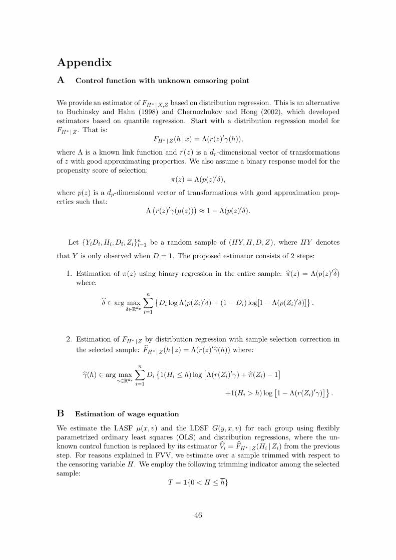
Appendix

A Control function with unknown censoring point

We provide an estimator of FH∗ |X,Z based on distribution regression. This is an alternativeto Buchinsky and Hahn (1998) and Chernozhukov and Hong (2002), which developedestimators based on quantile regression. Start with a distribution regression model forFH∗ |Z . That is:

FH∗ |Z(h |x) = Λ(r(z)′γ(h)),

where Λ is a known link function and r(z) is a dr-dimensional vector of transformationsof z with good approximating properties. We also assume a binary response model for thepropensity score of selection:

π(z) = Λ(p(z)′δ),

where p(z) is a dp-dimensional vector of transformations with good approximation prop-erties such that:

Λ(r(z)′γ(µ(z))

)≈ 1− Λ(p(z)′δ).

Let {YiDi,Hi,Di, Zi}ni=1 be a random sample of (HY,H,D,Z), where HY denotes

that Y is only observed when D = 1. The proposed estimator consists of 2 steps:

1. Estimation of π(z) using binary regression in the entire sample: π(z) = Λ(p(z)′δ)where:

δ ∈ arg maxδ∈Rdp

n∑

i=1

{Di log Λ(p(Zi)

′δ) + (1−Di) log[1− Λ(p(Zi)′δ)]

}.

2. Estimation of FH∗ |Z by distribution regression with sample selection correction in

the selected sample: FH∗ |Z(h | z) = Λ(r(z)′γ(h)) where:

γ(h) ∈ arg maxγ∈Rdr

n∑

i=1

Di

{1(Hi ≤ h) log

[Λ(r(Zi)

′γ) + π(Zi)− 1]

+1(Hi > h) log[1− Λ(r(Zi)

′γ)]}

.

B Estimation of wage equation

We estimate the LASF µ(x, v) and the LDSF G(y, x, v) for each group using flexiblyparametrized ordinary least squares (OLS) and distribution regressions, where the un-known control function is replaced by its estimator Vi = FH∗ |Z(Hi |Zi) from the previousstep. For reasons explained in FVV, we estimate over a sample trimmed with respect tothe censoring variable H. We employ the following trimming indicator among the selectedsample:

T = 1{0 < H ≤ h}

46

for some h ∈ (0,∞) such that P(T = 1) > 0. The estimator of the LASF is µ(x, v) =w(x, v)′β, where w(x, v) is a dw-dimensional vector of transformations of (x, v) with goodapproximating properties, and β is the OLS estimator:

β =

[n∑

i=1

Ti WiW′i

]−1 n∑

i=1

Ti WiYi,

where Wi = w(Xi, Vi). The estimator of the LDSF is G(y, x, v) = Λ(w(x, v)′β(y)), wherey ∈ R and β(y) is the logistic distribution regression estimator:

β(y) = arg maxb∈Rdw

n∑

i=1

Ti

[1{Yi ≤ y} log Λ(W ′

i b)) + 1{Yi > y} log Λ(−W ′i b))

].

Finally, in the third step we use (6) to estimate the counterfactual CDF (5) by:

GsY〈t,k,r〉

(y) =1

nskr

n∑

i=1

Λ(W ′i βt(y))1{Vi > 1− πr(Zi)},

where the average is taken over the sample values of Vi and Zi in group k, nskr =∑n

i=1 1{Vi > 1− πr(Zi)}, βt(y) is the logistic distribution regression estimator for group t

from the second step, and πr(z) is the estimator of the propensity score of selection forgroup r from the first step. Given Gs

Y〈t,k,r〉, we estimate the counterfactual QF (7) by:

qsY〈t,k,r〉(τ) =

∫ ∞

01{Gs

Y〈t,k,r〉(y) ≤ τ}dy −

∫ 0

−∞1{Gs

Y〈t,k,r〉(y) > τ}dy.

Following FVV, inference is based on the weighted bootstrap (Praestgaard and Wellner

1993). This method obtains the bootstrap version of the estimator of interest by repeating

all the estimation steps including sampling weights drawn from a nonnegative distribution

with mean and variance equal to one (e.g., standard exponential).

C Proof of Lemma 2

1

1− p

∫ 1

p

G(y, x, v)dv =1

1− p

∫ 1

p

P(g(x,E) ≤ y |V = v)dv

=

∫ 1

p

P(g(x,E) ≤ y |V = v)dFV |V >p(v)

= P(g(x,E) ≤ y |V > µh(z), Z = z, µh(Z) = p)

= P(Y ≤ y |H > h,X = x, µh(Z) = p),

The first equality is definition. The second equality uses V ∼ U(0, 1) and the third equality

uses independence of (E,V ) and Z. The final equality uses the definitions of Y and H

and is identified because (x, p) ∈ XPK .

47

D Derivations of equation (12)

Adapting the representation of the distribution of the observed Y in Section 3.2 to

the ordered selection rules yields

GsY (y) =

∫Zk

∫G(y, x, v)1{v > µ0(z)}dvdFZ(z)∫Zk

∫1{v > µ0(z)} dvdFZ(z)

=

∑Kh=1

∫Zk

∫G(y, x, v)1{µh−1(z) < v ≤ µh(z)}dvdFZ(z)∫

Zk

∫1{v > µ0(z)} dvdFZ(z)

,

where the second equality uses that the interval (µ0(z), 1] is the union of the disjoint

intervals (µh−1(z), µh(z)], h = 1, . . . , K.

48

E Figures

1980 1990 2000 2010 2020−0.2

0

0.2

0.4

Year

Average

derivative

Hours Weeks

Figure E.1: Average derivative

1980 1990 2000 2010 2020−0.2

0

0.2

0.4

Year

ρtσ

Et

A. Only white FTFY females

1980 1990 2000 2010 2020−0.2

0

0.2

0.4

Year

B. All females

Figure E.2: Estimation of ρtσEtover time.

49

1980 1990 2000 2010

0

0.2

0.4

Year

Differen

ce

Total selection Term 1 Term 2 Term 3 Term 4

Figure E.3: Selection effect using the Heckman-selection model and the 4 parts ofthe selection effect are represented by (18); total sample is full population between24 and 65 and selected population is all workers working a positive number of hours.

1980 1990 2000 2010 2020−0.1

0

0.1

0.2

0.3

Year

Differen

ce

Selection Structural Composition Total

Figure E.4: Computation of the selection, composition and structural effect basedon equation (19)-(21); total sample is full population between 24 and 65 and selectedpopulation is all workers working a positive number of hours.

50

0.1

0.2

0.3

0.4

0.5

Average

Derivative

A. Our method

0

5 · 10−2

0.1

0.15

0.2B. Tobit

1980 1990 2000 2010 2020

−0.4

−0.2

0

0.2

Year

Average

Derivative

C. Propensity score

Figure E.5: Average derivative of the wage. A. is the derivative of our controlfunction, B. is the average derivative using derivatives of a Tobit, C. uses a non-separable sample selection model.

51