deep learning: approximation of functions by...
TRANSCRIPT

Deep Learning: Approximation of Functionsby Composition
Zuowei Shen
Department of MathematicsNational University of Singapore

Outline
1 A brief introduction of approximation theory
2 Deep learning: approximation of functions by composition
3 Approximation of CNNs and sparse coding
4 Approximation in feature space

Outline
1 A brief introduction of approximation theory
2 Deep learning: approximation of functions by composition
3 Approximation of CNNs and sparse coding
4 Approximation in feature space
A brief introduction of approximation theory
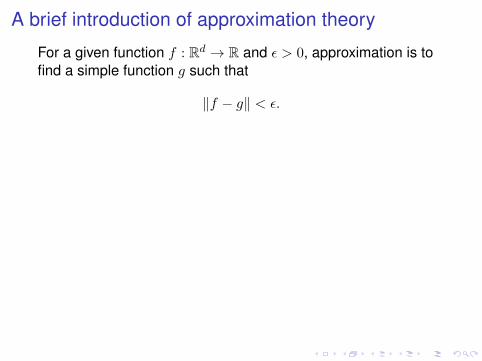
For a given function f : Rd → R and ε > 0, approximation is tofind a simple function g such that
‖f − g‖ < ε.
Function g : Rn → R can be as simple as g(x) = a · x. To makesense of this approximation, we need to find a mapT : Rd 7→ Rn, such that
‖f − g T‖ < ε.
1 Classical approximation: T is independent of data and ndepends on ε.
2 Deep learning: T depends on the data and n can beindependent of ε (T is learned from data).

A brief introduction of approximation theory
For a given function f : Rd → R and ε > 0, approximation is tofind a simple function g such that
‖f − g‖ < ε.
Function g : Rn → R can be as simple as g(x) = a · x. To makesense of this approximation, we need to find a mapT : Rd 7→ Rn, such that
‖f − g T‖ < ε.
1 Classical approximation: T is independent of data and ndepends on ε.
2 Deep learning: T depends on the data and n can beindependent of ε (T is learned from data).

Classical approximationLinear approximation: Given a finite set of generatorsφ1, . . . , φn, e.g. splines, wavelet frames, finite elements orgenerators in reproducing kernel Hilbert spaces. Define
T = [φ1, φ2, . . . , φn]> : Rd 7→ Rn and g(x) = a · x.
The linear approximation is to find a ∈ Rn such that
g T =
n∑i=1
aiφi ∼ f
It is linear because f1 ∼ g1, f2 ∼ g2 ⇒ f1 + f2 ∼ g1 + g2.
Nonlinear approximation: Given infinite generators Φ = φi∞i=1
and define
T = [φ1, φ2, . . . , ]> : Rd 7→∈ R∞ and g(x) = a · x
The nonlinear approximation of f is to find a finitely supported asuch that g T ∼ f .It is nonlinear because f1 ∼ g1, f2 ∼ g2 ; f1 + f2 ∼ g1 + g2 asthe support of the approximator g of f depends on f .

Classical approximationLinear approximation: Given a finite set of generatorsφ1, . . . , φn, e.g. splines, wavelet frames, finite elements orgenerators in reproducing kernel Hilbert spaces. Define
T = [φ1, φ2, . . . , φn]> : Rd 7→ Rn and g(x) = a · x.
The linear approximation is to find a ∈ Rn such that
g T =
n∑i=1
aiφi ∼ f
It is linear because f1 ∼ g1, f2 ∼ g2 ⇒ f1 + f2 ∼ g1 + g2.Nonlinear approximation: Given infinite generators Φ = φi∞i=1
and define
T = [φ1, φ2, . . . , ]> : Rd 7→∈ R∞ and g(x) = a · x
The nonlinear approximation of f is to find a finitely supported asuch that g T ∼ f .It is nonlinear because f1 ∼ g1, f2 ∼ g2 ; f1 + f2 ∼ g1 + g2 asthe support of the approximator g of f depends on f .

ExamplesConsider a function space L2(Rd), let φi∞i=1 be an orthonormalbasis of L2(Rd).
Linear approximationFor a given n, T = [φ1, . . . , φn]
> and g = a · x where aj = 〈f, φj〉. DenoteH = spanφ1, . . . , φn ⊆ L2(Rd).Then,
g T =
n∑i=1
〈f, φi〉φi
is the orthogonal projection onto the space H and is the best approximationof f from the space H.g T provides a good approximation of f when the sequence 〈f, φj〉∞j=1
decays fast as j → +∞.Therefore,
1 Linear approximation provides a good approximation for smoothfunctions.
2 When n =∞, it reproduces any function in L2(Rd).3 Advantage: It is a good approximation scheme for d is small, domain is
simple, function form is complicated but smooth.4 Disadvantage: if d is big and ε is small, n is huge.

ExamplesConsider a function space L2(Rd), let φi∞i=1 be an orthonormalbasis of L2(Rd).Linear approximationFor a given n, T = [φ1, . . . , φn]
> and g = a · x where aj = 〈f, φj〉. DenoteH = spanφ1, . . . , φn ⊆ L2(Rd).Then,
g T =n∑i=1
〈f, φi〉φi
is the orthogonal projection onto the space H and is the best approximationof f from the space H.
g T provides a good approximation of f when the sequence 〈f, φj〉∞j=1
decays fast as j → +∞.Therefore,
1 Linear approximation provides a good approximation for smoothfunctions.
2 When n =∞, it reproduces any function in L2(Rd).3 Advantage: It is a good approximation scheme for d is small, domain is
simple, function form is complicated but smooth.4 Disadvantage: if d is big and ε is small, n is huge.

ExamplesConsider a function space L2(Rd), let φi∞i=1 be an orthonormalbasis of L2(Rd).Linear approximationFor a given n, T = [φ1, . . . , φn]
> and g = a · x where aj = 〈f, φj〉. DenoteH = spanφ1, . . . , φn ⊆ L2(Rd).Then,
g T =n∑i=1
〈f, φi〉φi
is the orthogonal projection onto the space H and is the best approximationof f from the space H.g T provides a good approximation of f when the sequence 〈f, φj〉∞j=1
decays fast as j → +∞.
Therefore,1 Linear approximation provides a good approximation for smooth
functions.2 When n =∞, it reproduces any function in L2(Rd).3 Advantage: It is a good approximation scheme for d is small, domain is
simple, function form is complicated but smooth.4 Disadvantage: if d is big and ε is small, n is huge.

ExamplesConsider a function space L2(Rd), let φi∞i=1 be an orthonormalbasis of L2(Rd).Linear approximationFor a given n, T = [φ1, . . . , φn]
> and g = a · x where aj = 〈f, φj〉. DenoteH = spanφ1, . . . , φn ⊆ L2(Rd).Then,
g T =n∑i=1
〈f, φi〉φi
is the orthogonal projection onto the space H and is the best approximationof f from the space H.g T provides a good approximation of f when the sequence 〈f, φj〉∞j=1
decays fast as j → +∞.Therefore,
1 Linear approximation provides a good approximation for smoothfunctions.
2 When n =∞, it reproduces any function in L2(Rd).3 Advantage: It is a good approximation scheme for d is small, domain is
simple, function form is complicated but smooth.4 Disadvantage: if d is big and ε is small, n is huge.

Examples
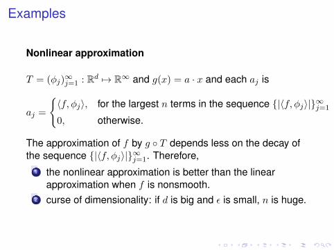
Nonlinear approximation
T = (φj)∞j=1 : Rd 7→ R∞ and g(x) = a · x and each aj is
aj =
〈f, φj〉, for the largest n terms in the sequence |〈f, φj〉|∞j=1
0, otherwise.
The approximation of f by g T depends less on the decay ofthe sequence |〈f, φj〉|∞j=1. Therefore,
1 the nonlinear approximation is better than the linearapproximation when f is nonsmooth.
2 curse of dimensionality: if d is big and ε is small, n is huge.
Examples
Nonlinear approximation
T = (φj)∞j=1 : Rd 7→ R∞ and g(x) = a · x and each aj is
aj =
〈f, φj〉, for the largest n terms in the sequence |〈f, φj〉|∞j=1
0, otherwise.
The approximation of f by g T depends less on the decay ofthe sequence |〈f, φj〉|∞j=1. Therefore,
1 the nonlinear approximation is better than the linearapproximation when f is nonsmooth.
2 curse of dimensionality: if d is big and ε is small, n is huge.

Both linear and nonlinear approximations are schemes toapproximate a class of function where T is fixed and itessentially changes a basis in order to represent orapproximate a certain class of functions.
Both linear and nonlinear approximations do not suit forapproximating f when f is defined on a complex domain, e.gmanifold in a very high dimensional space.
However, in deep learning, T is constructed by given data thatis adaptive to the underlying function to be approximated. Tchanges variables and maps domain of f to a feature domainwhere approximation become simpler, robust, and efficient.
Deep learning approximation is to find map T that maps thedomain of f to a “simple/ better domain” so that simpleclassical approximation can be applied.

Outline
1 A brief introduction of approximation theory
2 Deep learning: approximation of functions by composition
3 Approximation of CNNs and sparse coding
4 Approximation in feature space

Approximation for deep learning
Given data (xi, f(xi))mi=1.1 The key of deep learning is to construct a T by the given
data.2 T can simplify the domain of f through the change of
variables.3 T maps the key features of the domain of f and f , so that4 It is easy to find g s.t. g T gives a good approximation off .
What is the mathematics behind this?
Settings: construct a map T : Rd 7→ Rn and a simple function g(e.g. g = a · x ) from data such that g T provides a goodapproximation of f .

Approximation by compositions
Question 1: For arbitrarily given ε > 0, is there T : Rd 7→ Rsuch that ‖f − g T‖ ≤ ε?
Answer: Yes!
TheoremLet f : Rd → R and g : Rn → R and assume Im(f) ⊆ Im(g). Foran arbitrarily given ε > 0, there exists T : Rd 7→ Rn such that
‖f − g T‖ ≤ ε
T can be explicitly written out in terms of f and g.
T can be complex. This leads to

Approximation by compositions
Question 2: can T be a composition of simple maps? That is,can we write T = T1 · · · TJ and each Ti, i = 1, 2, . . . , J issimple, e.g. perturbation of identity.
Answer: Yes!
TheoremDenote f : Rd → R and g : Rn → R. For an arbitrarily givenε > 0, if Im(f) ⊆ Im(g), then there exists J simple mapsTi, i = 1, 2, . . . , J such that T = T1 T2 . . . TJ : Rd 7→ Rn and
‖f − g T1 · · · TJ‖ ≤ ε
Ti, i = 1, 2, . . . , J can be written out explicitly in terms of T .

Approximation by compositionsQuestion 3: Can Ti, i = 1, 2, . . . , J be mathematically constructed bysome scheme?Answer: Yes! Ti, i = 1, . . . , J can be constructed by solving theminimization problem:
minT1,T2,...,TJ
‖f − g T1 · · · TJ‖
A constructive proof is given in paper.
Question 4: Given training data xi, f(xi)mi=1, can we designnumerical scheme to find Ti, i = 1, 2 . . . , J and g such that
‖f − g T1 · · · TJ‖ ≤ ε, with high probability
by minimizing
1
m
m∑i=1
(f(xi)− g T1 · · · TJ(xi))2?
Answer: Yes! We do have designed deep neural networks for that.Numerical simulations show it performs well.

Approximation by compositionsQuestion 3: Can Ti, i = 1, 2, . . . , J be mathematically constructed bysome scheme?Answer: Yes! Ti, i = 1, . . . , J can be constructed by solving theminimization problem:
minT1,T2,...,TJ
‖f − g T1 · · · TJ‖
A constructive proof is given in paper.Question 4: Given training data xi, f(xi)mi=1, can we designnumerical scheme to find Ti, i = 1, 2 . . . , J and g such that
‖f − g T1 · · · TJ‖ ≤ ε, with high probability
by minimizing
1
m
m∑i=1
(f(xi)− g T1 · · · TJ(xi))2?
Answer: Yes! We do have designed deep neural networks for that.Numerical simulations show it performs well.

Ideas
One of the simplest ideas is
‖f − g T1 · · · TJ‖≤‖f − g T1 · · · TJ‖+ ‖g T1 · · · TJ − g T1 · · · TJ‖
=: Bias + Variance
Li, Shen and Tai, Deep learning: approximation of functions by composition, 2018.

This theory is complete, but does not answer all questions!For example, we do not have approximation order in terms ofthe number of nodes yet.
There are many different machine learning architectures, e.g.convolutional neural networks (CNNs) and sparse coding basedclassifiers, are different from the architecture we designed here.
Next, we will present approximation theory of CNNs and sparsecoding based classifiers for image classification.

Outline
1 A brief introduction of approximation theory
2 Deep learning: approximation of functions by composition
3 Approximation of CNNs and sparse coding
4 Approximation in feature space

Approximation for image classificationBinary classification
Ω = Ω0 ∪ Ω1 and Ω0 ∩ Ω1 = ∅.Let f to be the oracle classifier, i.e. f : Ω ⊂ Rd → 0, 1 and
f(x) =
0, if x ∈ Ω0,1, if x ∈ Ω1.
Construct feature map T and the classifier g such that
f − g T
is small.

Approximation for image classification
g is normally a fully connected layer followed by softmaxdefined on feature space.Construct a feature map T , so that g T approximates fwell, when constructing a fully connected layer toapproximate f from the data in image space is hard.
g T gives a good approximation of f if T satisfies
‖T (x)− T (y)‖ ≤ C‖x− y‖, ∀x, y ∈ Ω, (3.1)‖T (x)− T (y)‖ > c‖x− y‖, ∀x ∈ Ω0, y ∈ Ω1. (3.2)
for some C, c > 0.
The above inequalities are not easy to prove for both CNNs andsparse coding based classifiers especially when n ≤ d.

Accuracy of image classification of CNNsThe CNNs achieve desired classification accuracy with highprobability!All the numerical results confirmed it.
Settings:Given J sets of convolution kernels wiJi=1 and bias biJi=1.A J layer convolutional neural network is a nonlinear function
g T
whereT (x) = σ(wJ ~ σ(wJ−1 ~ · · · (σ(w1 ~ x+ b1)) · · ·+ bJ−1) + bJ)
g(x) =
n∑i=1
aiσ(w>i x+ bi), and σ(x) = max(0, x).
Normally, the convolutional kernels wiJi=1 have small size.Given m training samples (xi, yi)mi=1, T and a g are learned from
ming,T
1
m
m∑i=1
(yi − g T (xi))2.

Accuracy of image classification of CNNsThe CNNs achieve desired classification accuracy with highprobability!All the numerical results confirmed it.
Settings:Given J sets of convolution kernels wiJi=1 and bias biJi=1.A J layer convolutional neural network is a nonlinear function
g T
whereT (x) = σ(wJ ~ σ(wJ−1 ~ · · · (σ(w1 ~ x+ b1)) · · ·+ bJ−1) + bJ)
g(x) =
n∑i=1
aiσ(w>i x+ bi), and σ(x) = max(0, x).
Normally, the convolutional kernels wiJi=1 have small size.
Given m training samples (xi, yi)mi=1, T and a g are learned from
ming,T
1
m
m∑i=1
(yi − g T (xi))2.

Accuracy of image classification of CNNsThe CNNs achieve desired classification accuracy with highprobability!All the numerical results confirmed it.
Settings:Given J sets of convolution kernels wiJi=1 and bias biJi=1.A J layer convolutional neural network is a nonlinear function
g T
whereT (x) = σ(wJ ~ σ(wJ−1 ~ · · · (σ(w1 ~ x+ b1)) · · ·+ bJ−1) + bJ)
g(x) =
n∑i=1
aiσ(w>i x+ bi), and σ(x) = max(0, x).
Normally, the convolutional kernels wiJi=1 have small size.Given m training samples (xi, yi)mi=1, T and a g are learned from
ming,T
1
m
m∑i=1
(yi − g T (xi))2.

Accuracy of image classification of CNNs
Question: Whether can we have a rigorous proof for thisstatement?
Answer: Yes!
TheoremFor any given ε > 0 and sample data Z with sample size m, thereexists a CNN classifier whose filter size can be as small as 3, suchthat the classifier accuracy A satisfies
P(A ≥ 1− ε) ≥ 1− η(ε,m),
η(ε,m)→ 0 as m→ +∞.
The difficult part is to prove the inequalities (3.1) and (3.2) for T .
Bao, Shen, Tai, Wu and Xiang, Approximation and scaling analysis of convolutionalneural networks, 2017.

Accuracy of image classification of sparse codingGiven m training samples (xi, yi)mi=1, the sparse coding basedclassifier learn D and W via solving the problem
min‖dk‖=1,cimi=1,W
1
m
m∑i=1
‖xi −Dci‖2 + λ‖ci‖0 + γ‖yi −Wci‖2
There are numerical algorithms with global convergence property tosolve the above minimization.
The sparse coding based classifier is g T , where
g(x) = Wx and T (x) ∈ arg minc‖x− Dc‖2 + λ‖c‖0.
There is no mathematical analysis of classification accuracy of g T ,i.e. ‖f − g T‖.Bao, Ji, Quan, Shen, Dictionary learning for sparse coding: Algorithms and convergence analysis, IEEETransactions on Pattern Analysis and Machine Intelligence, 38(7), (2016), 1356-1369.Bao, Ji, Quan, Shen, L0 norm based dictionary learning by proximal methods with global convergence, IEEEConference Computer Vision and Pattern Recognition (CVPR), Columbus, (2014).

Accuracy of image classification of sparse coding
Consider an orthogonal dictionary learning (ODL) scheme
minD>D=I,cimi=1,g
1
m
m∑i=1
‖xi −Dci‖2 + λ‖ci‖1 + γ‖yi − g(ci)‖2
(3.3)
where g is a fully connected layer.The numerical algorithm to solve the above problem has globalconvergence property.
The classification accuracy is similar to the previous models.
Classification accuracies (%)Dataset K-SVD D-KSVD IDL ODL
Face: Extended Yale B 93.10 94.10 95.72 96.12Face: AR face 86.50 88.80 96.18 96.37
Object: Caltech101 68.70 68.60 72.29 72.54
For this model, we have mathematical analysis of accuracy.

Sparse coding approximation of image classification
Let g to be the fully connected layer and D is the dictionary fromsolving (3.3). Define
T (x) = arg minc‖x− Dc‖2 + λ‖c‖1.
The sparse coding based classifier from ODL model is g T .
TheoremConsider the ODL model. For any given ε > 0 and sample data Zwith sample size m, there exists a sparse coding based classifier,such that the classifier accuracy A satisfies
P(A ≥ 1− ε) ≥ 1− η(ε,m),
η(ε,m)→ 0 as m→ +∞.
To prove the two inequalities (3.1) and (3.2) of T is not easy.Bao, Ji and Shen, Classification accuracy of sparse coding based classifier, 2018.
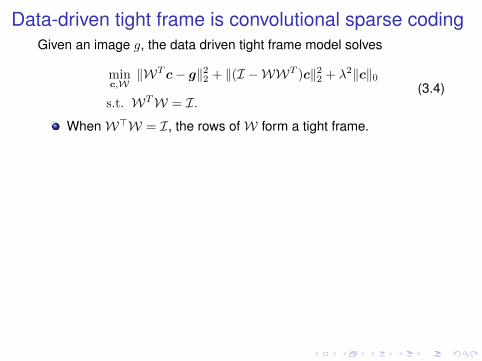
Data-driven tight frame is convolutional sparse codingGiven an image g, the data driven tight frame model solves
minc,W
‖WT c− g‖22 + ‖(I −WWT )c‖22 + λ2‖c‖0
s.t. WTW = I.(3.4)
WhenW>W = I, the rows ofW form a tight frame.
The minimization model (3.4) is equivalent to
minc,W
‖Wg − c‖22 + λ2‖c‖0, s.t. W>W = I. (3.5)
By the structure ofW, each channel ofW corresponds to aconvolutional kernel.
To solve (3.5), we use ADM. For fixedW, c can be solved byhard thresholding; For fixed c,W has an analytical solution andeasy to compute. Thanks the convolution structure ofW and thetight frame property.
The iteration algorithm converges.

Data-driven tight frame for image denoising
[1] Cai, Huang, Ji, Shen and Ye, Data-driven tight frame construction and image denois-ing, Applied and Computational Harmonic Analysis, 37(1), (2014), 89-105.[2] Bao, Ji and Shen, Convergence analysis for iterative data-driven tight frame construc-tion scheme, Applied and Computational Harmonic Analysis, 38(3), (2015), 510-523.

Outline
1 A brief introduction of approximation theory
2 Deep learning: approximation of functions by composition
3 Approximation of CNNs and sparse coding
4 Approximation in feature space

Back to classical approximation on feature domainClassical approximation is still useful for approximation infeature space.
Given noisy data xi, yimi=1 with
yi = (Sf)(xi) + ni,
where yimi=1 are samples of f with noise ni.
By applying some data fitting scheme, e.g., the waveletframe scheme, one obtains the denoised result
y∗i mi=1.
Let g be the function reconstructed by y∗i through someapproximation scheme.Question:1. What’s the error between g and f?2. Can we have g −→ f when the sampling data issufficiently dense?

Back to classical approximation on feature domainClassical approximation is still useful for approximation infeature space.
Given noisy data xi, yimi=1 with
yi = (Sf)(xi) + ni,
where yimi=1 are samples of f with noise ni.By applying some data fitting scheme, e.g., the waveletframe scheme, one obtains the denoised result
y∗i mi=1.
Let g be the function reconstructed by y∗i through someapproximation scheme.
Question:1. What’s the error between g and f?2. Can we have g −→ f when the sampling data issufficiently dense?

Back to classical approximation on feature domainClassical approximation is still useful for approximation infeature space.
Given noisy data xi, yimi=1 with
yi = (Sf)(xi) + ni,
where yimi=1 are samples of f with noise ni.By applying some data fitting scheme, e.g., the waveletframe scheme, one obtains the denoised result
y∗i mi=1.
Let g be the function reconstructed by y∗i through someapproximation scheme.Question:1. What’s the error between g and f?2. Can we have g −→ f when the sampling data issufficiently dense?

Data fitting
Let Ω := [0, 1]× [0, 1] and f ∈ L2(Ω). Let φ be the tensorproduct of B-spline functions and denote the scaled functionsby φn,α := 2nφ(2n · −α). Let (Sf)[α] = 2n〈f, φn,α〉.
Given noisy observations
y[α] = (Sf)[α] + nα, α = (α1, α2), 0 ≤ α1, α2 ≤ 2n − 1.
The data fitting problem is to recover f on Ω from y.

Wavelet frameLet φ be a refinable function and Ψ := ψi, i = 1, . . . , r bethe wavelet functions associated with φ in L2(R2).
Denote the scaled functions by
φn,α := 2nφ(2n · −α) and ψi,n,α := 2nψi(2n · −α).
X(Ψ) := ψi,n,α is a tight frame if
‖f‖22 =∑i,n,α
|〈f, ψi,n,α〉|2, ∀f ∈ L2(R).
Unitary extension principle (UEP): Assume the masks hisatisfy the following equalities
2r∑i=0
∑k∈Z
hi(m+ 2k + `)hi(2k + `) = δm, for any m, ` ∈ Z,
X(Ψ) := ψi,n,α is a tight frame.Ron and Shen, Affine systems in L2(Rd): the analysis of the analysis operator, Journalof Functional Analysis, 148(2), (1997), 408-447.Daubechies, Han, Ron and Shen, Framelets: MRA-based constructions of waveletframes, Applied and Computational Harmonic Analysis, 14(1), (2003), 1-46.

Wavelet frameLet φ be a refinable function and Ψ := ψi, i = 1, . . . , r bethe wavelet functions associated with φ in L2(R2).Denote the scaled functions by
φn,α := 2nφ(2n · −α) and ψi,n,α := 2nψi(2n · −α).
X(Ψ) := ψi,n,α is a tight frame if
‖f‖22 =∑i,n,α
|〈f, ψi,n,α〉|2, ∀f ∈ L2(R).
Unitary extension principle (UEP): Assume the masks hisatisfy the following equalities
2
r∑i=0
∑k∈Z
hi(m+ 2k + `)hi(2k + `) = δm, for any m, ` ∈ Z,
X(Ψ) := ψi,n,α is a tight frame.
Ron and Shen, Affine systems in L2(Rd): the analysis of the analysis operator, Journalof Functional Analysis, 148(2), (1997), 408-447.Daubechies, Han, Ron and Shen, Framelets: MRA-based constructions of waveletframes, Applied and Computational Harmonic Analysis, 14(1), (2003), 1-46.

Wavelet frameLet φ be a refinable function and Ψ := ψi, i = 1, . . . , r bethe wavelet functions associated with φ in L2(R2).Denote the scaled functions by
φn,α := 2nφ(2n · −α) and ψi,n,α := 2nψi(2n · −α).
X(Ψ) := ψi,n,α is a tight frame if
‖f‖22 =∑i,n,α
|〈f, ψi,n,α〉|2, ∀f ∈ L2(R).
Unitary extension principle (UEP): Assume the masks hisatisfy the following equalities
2
r∑i=0
∑k∈Z
hi(m+ 2k + `)hi(2k + `) = δm, for any m, ` ∈ Z,
X(Ψ) := ψi,n,α is a tight frame.Ron and Shen, Affine systems in L2(Rd): the analysis of the analysis operator, Journalof Functional Analysis, 148(2), (1997), 408-447.Daubechies, Han, Ron and Shen, Framelets: MRA-based constructions of waveletframes, Applied and Computational Harmonic Analysis, 14(1), (2003), 1-46.

Examples of spline wavelets from UEP
Piecewise linear refinable B-spline and the corresponding framelets.
Refinement mask h0 = [ 14, 12, 14]. High pass filters h1 = [− 1
4, 12,− 1
4] and h2 = [
√2
4, 0,−
√2
4].
Piecewise cubic refinable B-spline and the corresponding framelets.
Refinement mask h0 = [ 116, 14, 38, 14, 116
]. High pass filters h1 = [ 116,− 1
4, 38,− 1
4, 116
],
h2 = [− 18, 14, 0,− 1
4, 18], h3 = [
√6
16, 0,−
√6
8, 0,
√6
16] and h4 = [− 1
8,− 1
4, 0, 1
4, 18].
Discrete wavelet transformW:
an,α := 〈f, φn,α〉W−→ 〈f, ψi,n,α〉ri=0 = hi ∗ an,αri=0,
where hi are the wavelet frame filters.

Wavelet frame based data fitting scheme
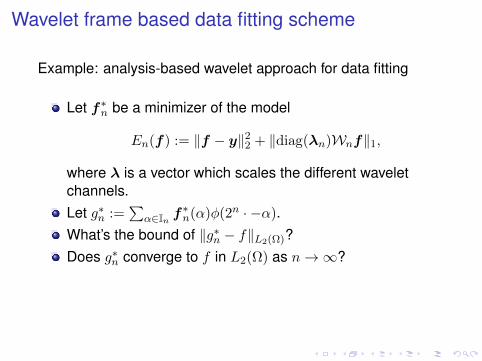
Example: analysis-based wavelet approach for data fitting
Let f∗n be a minimizer of the model
En(f) := ‖f − y‖22 + ‖diag(λn)Wnf‖1,
where λ is a vector which scales the different waveletchannels.
Let g∗n :=∑
α∈In f∗n(α)φ(2n · −α).
What’s the bound of ‖g∗n − f‖L2(Ω)?Does g∗n converge to f in L2(Ω) as n→∞?

Wavelet frame based data fitting scheme
Example: analysis-based wavelet approach for data fitting
Let f∗n be a minimizer of the model
En(f) := ‖f − y‖22 + ‖diag(λn)Wnf‖1,
where λ is a vector which scales the different waveletchannels.Let g∗n :=
∑α∈In f
∗n(α)φ(2n · −α).
What’s the bound of ‖g∗n − f‖L2(Ω)?
Does g∗n converge to f in L2(Ω) as n→∞?
Wavelet frame based data fitting scheme
Example: analysis-based wavelet approach for data fitting
Let f∗n be a minimizer of the model
En(f) := ‖f − y‖22 + ‖diag(λn)Wnf‖1,
where λ is a vector which scales the different waveletchannels.Let g∗n :=
∑α∈In f
∗n(α)φ(2n · −α).
What’s the bound of ‖g∗n − f‖L2(Ω)?Does g∗n converge to f in L2(Ω) as n→∞?

Regularity assumption of f : There exits β > −1 such that∑α
|〈f, φ0,α〉|+∑n≥0
2βn∑i,α
|〈f, ψi,n,α〉| <∞.
Then for an arbitrary given 0 < δ < 1, the followinginequality
‖g∗n − f‖L2(Ω) ≤ C12−nmin 1+β2, 12 log
1
δ+ C2σ
2
holds with confidence 1− δ.When n→∞, one can design a data fitting scheme suchthat
limn→∞
E(‖g∗n − f‖L2(Ω)
)= 0.
In this case, data is given on uniform grids.

Regularity assumption of f : There exits β > −1 such that∑α
|〈f, φ0,α〉|+∑n≥0
2βn∑i,α
|〈f, ψi,n,α〉| <∞.
Then for an arbitrary given 0 < δ < 1, the followinginequality
‖g∗n − f‖L2(Ω) ≤ C12−nmin 1+β2, 12 log
1
δ+ C2σ
2
holds with confidence 1− δ.
When n→∞, one can design a data fitting scheme suchthat
limn→∞
E(‖g∗n − f‖L2(Ω)
)= 0.
In this case, data is given on uniform grids.

Regularity assumption of f : There exits β > −1 such that∑α
|〈f, φ0,α〉|+∑n≥0
2βn∑i,α
|〈f, ψi,n,α〉| <∞.
Then for an arbitrary given 0 < δ < 1, the followinginequality
‖g∗n − f‖L2(Ω) ≤ C12−nmin 1+β2, 12 log
1
δ+ C2σ
2
holds with confidence 1− δ.When n→∞, one can design a data fitting scheme suchthat
limn→∞
E(‖g∗n − f‖L2(Ω)
)= 0.
In this case, data is given on uniform grids.

Regularity assumption of f : There exits β > −1 such that∑α
|〈f, φ0,α〉|+∑n≥0
2βn∑i,α
|〈f, ψi,n,α〉| <∞.
Then for an arbitrary given 0 < δ < 1, the followinginequality
‖g∗n − f‖L2(Ω) ≤ C12−nmin 1+β2, 12 log
1
δ+ C2σ
2
holds with confidence 1− δ.When n→∞, one can design a data fitting scheme suchthat
limn→∞
E(‖g∗n − f‖L2(Ω)
)= 0.
In this case, data is given on uniform grids.

When the noisy data are obtained from nonuniform grids orobtained by random sampling, can we have a similarresult?
Yes. It is technical but it has been carefully studied.
Cai, Shen and Ye, Approximation of frame based missing data recovery, Applied and Computational Harmonic
Analysis, 31(2), (2011), 185-204.
Yang, Stahl and Shen, An analysis of wavelet frame based scattered data reconstruction, Applied and
Computational Harmonic Analysis, 42(3), (2017), 480-507.
Yang, Dong and Shen, Approximation of analog signals from noisy data, manuscript, 2018.

When the noisy data are obtained from nonuniform grids orobtained by random sampling, can we have a similarresult?Yes. It is technical but it has been carefully studied.
Cai, Shen and Ye, Approximation of frame based missing data recovery, Applied and Computational Harmonic
Analysis, 31(2), (2011), 185-204.
Yang, Stahl and Shen, An analysis of wavelet frame based scattered data reconstruction, Applied and
Computational Harmonic Analysis, 42(3), (2017), 480-507.
Yang, Dong and Shen, Approximation of analog signals from noisy data, manuscript, 2018.

Thank you!
http://www.math.nus.edu.sg/∼matzuows/