deep learning with azure - programmer books...pooling layer activation functions 136 ... he holds a...
TRANSCRIPT

Deep Learning with Azure
Building and Deploying Artificial Intelligence Solutions on the Microsoft AI Platform—Mathew SalvarisDanielle DeanWee Hyong Tok
www.allitebooks.com
Deep Learning with Azure
Building and Deploying Artificial Intelligence Solutions
on the Microsoft AI Platform
Mathew SalvarisDanielle DeanWee Hyong Tok
www.allitebooks.com
Deep Learning with Azure
ISBN-13 (pbk): 978-1-4842-3678-9 ISBN-13 (electronic): 978-1-4842-3679-6 https://doi.org/10.1007/978-1-4842-3679-6
Library of Congress Control Number: 2018953705
Copyright © 2018 by Mathew Salvaris, Danielle Dean, Wee Hyong Tok
This work is subject to copyright. All rights are reserved by the Publisher, whether the whole or part of the material is concerned, specifically the rights of translation, reprinting, reuse of illustrations, recitation, broadcasting, reproduction on microfilms or in any other physical way, and transmission or information storage and retrieval, electronic adaptation, computer software, or by similar or dissimilar methodology now known or hereafter developed.
Trademarked names, logos, and images may appear in this book. Rather than use a trademark symbol with every occurrence of a trademarked name, logo, or image we use the names, logos, and images only in an editorial fashion and to the benefit of the trademark owner, with no intention of infringement of the trademark.
The use in this publication of trade names, trademarks, service marks, and similar terms, even if they are not identified as such, is not to be taken as an expression of opinion as to whether or not they are subject to proprietary rights.
While the advice and information in this book are believed to be true and accurate at the date of publication, neither the authors nor the editors nor the publisher can accept any legal responsibility for any errors or omissions that may be made. The publisher makes no warranty, express or implied, with respect to the material contained herein.
Managing Director, Apress Media LLC: Welmoed SpahrAcquisitions Editor: Joan MurrayDevelopment Editor: Laura BerendsonCoordinating Editor: Jill Balzano
Cover designed by eStudioCalamar
Cover image designed by Freepik (www.freepik.com)
Distributed to the book trade worldwide by Springer Science+Business Media New York, 233 Spring Street, 6th Floor, New York, NY 10013. Phone 1-800-SPRINGER, fax (201) 348-4505, e-mail [email protected], or visit www.springeronline.com. Apress Media, LLC is a California LLC and the sole member (owner) is Springer Science + Business Media Finance Inc (SSBM Finance Inc). SSBM Finance Inc is a Delaware corporation.
For information on translations, please e-mail [email protected], or visit http://www.apress.com/rights-permissions.
Apress titles may be purchased in bulk for academic, corporate, or promotional use. eBook versions and licenses are also available for most titles. For more information, reference our Print and eBook Bulk Sales web page at http://www.apress.com/bulk-sales.
Any source code or other supplementary material referenced by the author in this book is available to readers on GitHub via the book's product page, located at www.apress.com/9781484236789. For more detailed information, please visit http://www.apress.com/source-code.
Printed on acid-free paper
Mathew SalvarisLondon, United Kingdom
Danielle DeanWestford, Massachusetts, USA
Wee Hyong TokRedmond, Washington, USA
www.allitebooks.com

Dedicated to our families and friends who supported us as we took away from our personal time
to learn, develop, and write materials for this book.
Special dedication to Juliet, Nathaniel, Jayden, and Adrian
www.allitebooks.com
v
Table of Contents
Part I: Getting Started with AI ����������������������������������������������1
Chapter 1: Introduction to Artificial Intelligence ����������������������������������3
Microsoft and AI ����������������������������������������������������������������������������������������������������6
Machine Learning �������������������������������������������������������������������������������������������������9
Deep Learning �����������������������������������������������������������������������������������������������������14
Rise of Deep Learning �����������������������������������������������������������������������������������16
Applications of Deep Learning �����������������������������������������������������������������������21
Summary�������������������������������������������������������������������������������������������������������������25
Chapter 2: Overview of Deep Learning �����������������������������������������������27
Common Network Structures ������������������������������������������������������������������������������28
Convolutional Neural Networks ���������������������������������������������������������������������29
Recurrent Neural Networks ���������������������������������������������������������������������������33
Generative Adversarial Networks ������������������������������������������������������������������35
Autoencoders ������������������������������������������������������������������������������������������������36
About the Authors ������������������������������������������������������������������������������xiii
About the Guest Authors of Chapter 7 ������������������������������������������������xv
About the Technical Reviewers ��������������������������������������������������������xvii
Acknowledgments �����������������������������������������������������������������������������xix
Foreword �������������������������������������������������������������������������������������������xxi
Introduction ��������������������������������������������������������������������������������������xxv
www.allitebooks.com
vi
Deep Learning Workflow �������������������������������������������������������������������������������������37
Finding Relevant Data Set(s) �������������������������������������������������������������������������38
Data Set Preprocessing ���������������������������������������������������������������������������������39
Training the Model �����������������������������������������������������������������������������������������40
Validating and Tuning the Model �������������������������������������������������������������������40
Deploy the Model �������������������������������������������������������������������������������������������42
Deep Learning Frameworks & Compute ��������������������������������������������������������43
Jump Start Deep Learning: Transfer Learning and Domain Adaptation ���������47
Models Library �����������������������������������������������������������������������������������������������50
Summary�������������������������������������������������������������������������������������������������������������51
Chapter 3: Trends in Deep Learning ����������������������������������������������������53
Variations on Network Architectures �������������������������������������������������������������������53
Residual Networks and Variants �������������������������������������������������������������������54
DenseNet ������������������������������������������������������������������������������������������������������54
Small Models, Fewer Parameters �����������������������������������������������������������������55
Capsule Networks �����������������������������������������������������������������������������������������56
Object Detection �������������������������������������������������������������������������������������������58
Object Segmentation �������������������������������������������������������������������������������������60
More Sophisticated Networks ����������������������������������������������������������������������60
Automated Machine Learning ����������������������������������������������������������������������61
Hardware �����������������������������������������������������������������������������������������������������������63
More Specialized Hardware���������������������������������������������������������������������������64
Hardware on Azure ����������������������������������������������������������������������������������������65
Quantum Computing �������������������������������������������������������������������������������������65
Limitations of Deep Learning ������������������������������������������������������������������������������67
Be Wary of Hype ��������������������������������������������������������������������������������������������67
Limits on Ability to Generalize �����������������������������������������������������������������������68
Table of ConTenTsTable of ConTenTs

vii
Data Hungry Models, Especially Labels ���������������������������������������������������������70
Reproducible Research and Underlying Theory ��������������������������������������������70
Looking Ahead: What Can We Expect from Deep Learning? �������������������������������72
Ethics and Regulations ���������������������������������������������������������������������������������73
Summary�������������������������������������������������������������������������������������������������������������75
Part II: Azure AI Platform and Experimentation Tools ��������77
Chapter 4: Microsoft AI Platform ��������������������������������������������������������79
Services ��������������������������������������������������������������������������������������������������������������81
Prebuilt AI: Cognitive Services �����������������������������������������������������������������������82
Conversational AI: Bot Framework ����������������������������������������������������������������84
Custom AI: Azure Machine Learning Services �����������������������������������������������84
Custom AI: Batch AI ���������������������������������������������������������������������������������������85
Infrastructure ������������������������������������������������������������������������������������������������������86
Data Science Virtual Machine ������������������������������������������������������������������������87
Spark �������������������������������������������������������������������������������������������������������������88
Container Hosting ������������������������������������������������������������������������������������������89
Data Storage ��������������������������������������������������������������������������������������������������91
Tools ��������������������������������������������������������������������������������������������������������������������92
Azure Machine Learning Studio ���������������������������������������������������������������������92
Integrated Development Environments ���������������������������������������������������������93
Deep Learning Frameworks ��������������������������������������������������������������������������93
Broader Azure Platform ���������������������������������������������������������������������������������������94
Getting Started with the Deep Learning Virtual Machine ������������������������������������95
Running the Notebook Server �����������������������������������������������������������������������97
Summary�������������������������������������������������������������������������������������������������������������98
Table of ConTenTsTable of ConTenTs
viii
Chapter 5: Cognitive Services and Custom Vision ������������������������������99
Prebuilt AI: Why and How? ����������������������������������������������������������������������������������99
Cognitive Services ��������������������������������������������������������������������������������������������101
What Types of Cognitive Services Are Available? ����������������������������������������������104
Computer Vision APIs �����������������������������������������������������������������������������������106
How Do I Get Started with Cognitive Services? ������������������������������������������������113
Custom Vision ���������������������������������������������������������������������������������������������������119
Hello World! for Custom Vision ��������������������������������������������������������������������120
Exporting Custom Vision Models �����������������������������������������������������������������127
Summary�����������������������������������������������������������������������������������������������������������128
Part III: AI Networks in Practice ���������������������������������������129
Chapter 6: Convolutional Neural Networks ���������������������������������������131
The Convolution in Convolution Neural Networks ���������������������������������������������132
Convolution Layer ����������������������������������������������������������������������������������������134
Pooling Layer �����������������������������������������������������������������������������������������������135
Activation Functions ������������������������������������������������������������������������������������136
CNN Architecture �����������������������������������������������������������������������������������������������139
Training Classification CNN �������������������������������������������������������������������������������140
Why CNNs ���������������������������������������������������������������������������������������������������������142
Training CNN on CIFAR10 ����������������������������������������������������������������������������������143
Training a Deep CNN on GPU �����������������������������������������������������������������������������150
Model 1 ��������������������������������������������������������������������������������������������������������151
Model 2 ��������������������������������������������������������������������������������������������������������152
Model 3 ��������������������������������������������������������������������������������������������������������154
Model 4 ��������������������������������������������������������������������������������������������������������156
Transfer Learning ����������������������������������������������������������������������������������������������159
Summary�����������������������������������������������������������������������������������������������������������160
Table of ConTenTsTable of ConTenTs
ix
Chapter 7: Recurrent Neural Networks ���������������������������������������������161
RNN Architectures ���������������������������������������������������������������������������������������������164
Training RNNs ���������������������������������������������������������������������������������������������������169
Gated RNNs �������������������������������������������������������������������������������������������������������170
Sequence-to-Sequence Models and Attention Mechanism ������������������������������172
RNN Examples ��������������������������������������������������������������������������������������������������176
Example 1: Sentiment Analysis �������������������������������������������������������������������176
Example 2: Image Classification ������������������������������������������������������������������176
Example 3: Time Series �������������������������������������������������������������������������������180
Summary�����������������������������������������������������������������������������������������������������������186
Chapter 8: Generative Adversarial Networks �����������������������������������187
What Are Generative Adversarial Networks? ����������������������������������������������������188
Cycle-Consistent Adversarial Networks ������������������������������������������������������������194
The CycleGAN Code �������������������������������������������������������������������������������������196
Network Architecture for the Generator and Discriminator �������������������������200
Defining the CycleGAN Class �����������������������������������������������������������������������204
Adversarial and Cyclic Loss �������������������������������������������������������������������������206
Results ��������������������������������������������������������������������������������������������������������������207
Summary�����������������������������������������������������������������������������������������������������������208
Part IV: AI Architectures and Best Practices ��������������������209
Chapter 9: Training AI Models ����������������������������������������������������������211
Training Options ������������������������������������������������������������������������������������������������211
Distributed Training �������������������������������������������������������������������������������������212
Deep Learning Virtual Machine��������������������������������������������������������������������213
Table of ConTenTsTable of ConTenTs
x
Batch Shipyard ��������������������������������������������������������������������������������������������215
Batch AI �������������������������������������������������������������������������������������������������������216
Deep Learning Workspace ���������������������������������������������������������������������������217
Examples to Follow Along ���������������������������������������������������������������������������������218
Training DNN on Batch Shipyard �����������������������������������������������������������������218
Azure Machine Learning Services ���������������������������������������������������������������239
Other Options for AI Training on Azure ���������������������������������������������������������240
Summary�����������������������������������������������������������������������������������������������������������241
Chapter 10: Operationalizing AI Models �������������������������������������������243
Operationalization Platforms �����������������������������������������������������������������������������243
DLVM �����������������������������������������������������������������������������������������������������������������245
Azure Container Instances ���������������������������������������������������������������������������245
Azure Web Apps �������������������������������������������������������������������������������������������247
Azure Kubernetes Services �������������������������������������������������������������������������247
Azure Service Fabric �����������������������������������������������������������������������������������250
Batch AI �������������������������������������������������������������������������������������������������������251
AZTK ������������������������������������������������������������������������������������������������������������252
HDInsight and Databricks ����������������������������������������������������������������������������254
SQL Server ���������������������������������������������������������������������������������������������������255
Operationalization Overview �����������������������������������������������������������������������������255
Azure Machine Learning Services���������������������������������������������������������������������258
Summary�����������������������������������������������������������������������������������������������������������259
Table of ConTenTsTable of ConTenTs
xi
Appendix: Notes ��������������������������������������������������������������������������������261
Chapter 1 ����������������������������������������������������������������������������������������������������������261
Chapter 2 ����������������������������������������������������������������������������������������������������������264
Chapter 3 ����������������������������������������������������������������������������������������������������������265
Chapter 4 ����������������������������������������������������������������������������������������������������������270
Chapter 5 ����������������������������������������������������������������������������������������������������������270
Chapter 6 ����������������������������������������������������������������������������������������������������������270
Chapter 7 ����������������������������������������������������������������������������������������������������������272
Chapter 8 ����������������������������������������������������������������������������������������������������������274
Chapter 9 ����������������������������������������������������������������������������������������������������������275
Chapter 10 ��������������������������������������������������������������������������������������������������������276
Index �������������������������������������������������������������������������������������������������277
Table of ConTenTsTable of ConTenTs
xiii
About the Authors
Mathew Salvaris, PhD is a senior data scientist
at Microsoft in Azure CAT, where he works
with a team of data scientists and engineers
building machine learning and AI solutions for
external companies utilizing Microsoft’s Cloud
AI platform. He enlists the latest innovations
in machine learning and deep learning to
deliver novel solutions for real-world business
problems, and to leverage learning from
these engagements to help improve Microsoft’s Cloud AI products. Prior
to joining Microsoft, he worked as a data scientist for a fintech startup,
where he specialized in providing machine learning solutions. Previously,
he held a postdoctoral research position at University College London in
the Institute of Cognitive Neuroscience, where he used machine learning
methods and electroencephalography to investigate volition. Prior to
that position, he worked as a postdoctoral researcher in brain–computer
interfaces at the University of Essex. Mathew holds a PhD and MSc in
computer science.
Danielle Dean, PhD is a principal data science
lead at Microsoft in Azure CAT, where she
leads a team of data scientists and engineers
building artificial intelligence solutions with
external companies utilizing Microsoft’s Cloud
AI platform. Previously, she was a data scientist
at Nokia, where she produced business value
and insights from big data through data mining

xiv
and statistical modeling on data-driven projects that affected a range
of businesses, products, and initiatives. She has a PhD in quantitative
psychology from the University of North Carolina at Chapel Hill, where she
studied the application of multilevel event history models to understand
the timing and processes leading to events between dyads within social
networks.
Wee Hyong Tok, PhD is a principal data science manager at Microsoft in
the Cloud and AI division. He leads the AI for Earth Engineering and Data
Science team, a team of data scientists and engineers who are working
to advance the boundaries of state-of-the-art deep learning algorithms
and systems. His team works extensively with deep learning frameworks,
ranging from TensorFlow to CNTK, Keras, and PyTorch. He has worn
many hats in his career as developer, program and product manager,
data scientist, researcher, and strategist. Throughout his career, he has
been a trusted advisor to the C-suite, from Fortune 500 companies to
startups. He coauthored one of the first books on Azure machine learning,
Predictive Analytics Using Azure Machine Learning, and authored another
demonstrating how database professionals can do AI with databases,
Doing Data Science with SQL Server. He has a PhD in computer science
from the National University of Singapore, where he studied progressive
join algorithms for data streaming systems.
abouT The auThorsabouT The auThors
xv
About the Guest Authors of Chapter 7
Ilia Karmanov writes code and does
data science for Microsoft. He also models
part-time for indoor bouldering.
Miguel González-Fierro, PhD is a data
scientist in AzureCAT at Microsoft UK, where
his job consists of helping customers leverage
their processes using big data and machine
learning. Previously, he was CEO and founder
of Samsamia Technologies, a company that
created a visual search engine for fashion items
allowing users to find products using images
instead of words, and founder of the Robotics
Society of Universidad Carlos III, which developed different projects
related to UAVs, mobile robots, small humanoids competitions, and 3D
printers. Miguel also worked as a robotics scientist at Universidad Carlos
III of Madrid and King’s College London, where his research focused on
learning from demonstration, reinforcement learning, computer vision,
and dynamic control of humanoid robots. He holds a BSc and MSc in
electrical engineering and an MSc and PhD in robotics.

xvii
Mary Wahl, PhD is a data scientist at Microsoft
within AzureCAT in the Cloud and AI division.
She currently works on helping conservation
science nongovernmental organizations
apply machine learning to geospatial data and
imagery through the AI for Earth initiative. She
previously worked in the Algorithms and Data
Science Solutions Team within Microsoft’s AI
and Research Group, where she developed
custom machine learning pipelines for enterprise customers. Mary holds
her PhD in molecular and cellular biology from Harvard University.
Thomas Delteil is an applied scientist
currently employed at Amazon in the AWS
Deep Learning team. He has a background in
machine learning and software engineering
and previously worked for the Microsoft
Cloud AI team as an applied scientist. He
holds an MSc from Imperial College London
in advanced computing and another MSc
from ISAE-Supaero, Toulouse, in aerospace
engineering.
About the Technical Reviewers
xix
Acknowledgments
Thank you to Ilia Karmanov and Miguel González-Fierro for writing
Chapter 7, “Recurrent Neural Networks,” and for many suggestions for
improvement across the rest of the book. Thanks also to Mary Wahl and
Thomas Delteil for their technical review of the book; the book wouldn’t
be the same without them. Finally, thank you to our many colleagues who
developed, shaped, and used the products and techniques mentioned in
this book that influenced our presentation of them.
xxi
Foreword
Artificial intelligence (AI) at its core is about empowering people and
organizations to reason and interact with the increasingly digital world
all around us. Whether it be in health care or in financial services or in
government, AI is helping transform customer experiences, business
models, and operational efficiencies in a dramatic way. In this book,
Mathew, Danielle, and Wee Hyong present a practical overview of why the
impact of AI and deep learning has accelerated recently and illustrate how
to build these solutions on the Microsoft Cloud AI platform. They build on
their experiences as leading data scientists at Microsoft working both with
the product group as well as with external customers. In this book you will
see a fresh perspective on how to approach building AI solutions: from the
common types of models to training and deployment considerations for
end-to-end systems.
This topic is very near to my heart. As a Corporate Vice President
and CTO of Artifical Intelligence at Microsoft, I have had the privilege of
leading the development of many of our AI products mentioned in this
book. Take Unilever, for example: They have built a collection of chat bots
with a master bot to help their employees interact with human resources
services and all services inside the enterprise. Jabil uses AI for quality
control in the circuit board manufacturing process. Cochrane uses AI
to classify medical documents and organize information for systematic
reviews. Publicis used AI to build an app for makeup recommendations.
eSmart Systems has a connected drone with deep learning-based defect
detection for inspecting power lines in the energy sector. AI is even being
used to identify and conserve snow leopards in the Himalayas. AI is
becoming the new normal.

xxii
Contrast these examples to enterprise IT systems of the past. We first
developed systems of record for enterprises to operate. We had enterprise
resource planning (ERP) systems. We had customer resource management
(CRM) systems. Most of these were rather siloed and served specific
individual functions, with highly structured and curated data. Then the
Web came along, and the Internet came along, and we built systems to
interact with our customers over the Web. We started building Software as
a Service (SaaS) applications hosted in the cloud.
Now what we have at our disposal thanks to the type of technologies
and techniques mentioned in this book are systems of intelligence in the cloud. A system of intelligence integrates data across all those systems
of record, connects you to the systems of engagement, and creates a
connected enterprise that understands, reasons, and interacts in a very
natural way. Built as a collection of interoperating SaaS applications, these
systems collect and organize all relevant data and interactions in the cloud.
They constantly learn using AI and deliver new experiences. Live online
experiments constantly explore a space of possibilities to teach and derive
new AI capabilities. All this is done with the power of the cloud.
When you are building powerful systems like this, you need a very
comprehensive platform. It’s not just one or two components, or a
few components from open source integrated with existing enterprise
applications. You can’t just take a deep learning tool, learn with a little
bit of data, put the model in a virtual machine on the cloud, and build a
system of intelligence. You need a comprehensive collection of platform
services that only a cloud platform can bring, including systems for identity
and security. This is the differentiation of the Microsoft AI platform. It is
cloud-powered AI for next-generation systems of intelligence.
I am a big believer in democratizing AI for developers. A lot of AI
itself should be almost as simple as calling a sort function. You just call a
sort function, and you get an output. The Microsoft AI platform provides
a wealth of prebuilt AI like speech recognition, translation, image
understanding, optical character recognition (OCR), and handwriting
forewordforeword
xxiii
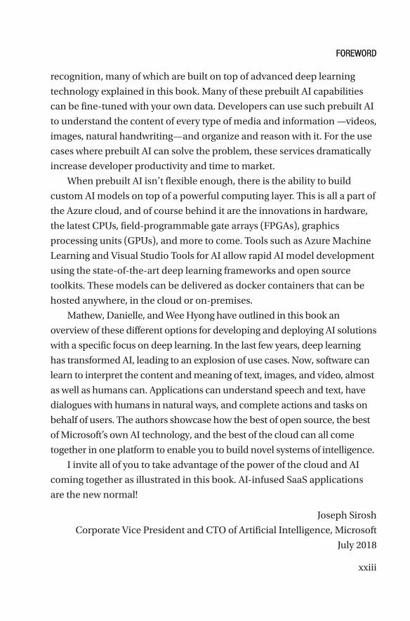
recognition, many of which are built on top of advanced deep learning
technology explained in this book. Many of these prebuilt AI capabilities
can be fine-tuned with your own data. Developers can use such prebuilt AI
to understand the content of every type of media and information —videos,
images, natural handwriting—and organize and reason with it. For the use
cases where prebuilt AI can solve the problem, these services dramatically
increase developer productivity and time to market.
When prebuilt AI isn’t flexible enough, there is the ability to build
custom AI models on top of a powerful computing layer. This is all a part of
the Azure cloud, and of course behind it are the innovations in hardware,
the latest CPUs, field-programmable gate arrays (FPGAs), graphics
processing units (GPUs), and more to come. Tools such as Azure Machine
Learning and Visual Studio Tools for AI allow rapid AI model development
using the state-of-the-art deep learning frameworks and open source
toolkits. These models can be delivered as docker containers that can be
hosted anywhere, in the cloud or on-premises.
Mathew, Danielle, and Wee Hyong have outlined in this book an
overview of these different options for developing and deploying AI solutions
with a specific focus on deep learning. In the last few years, deep learning
has transformed AI, leading to an explosion of use cases. Now, software can
learn to interpret the content and meaning of text, images, and video, almost
as well as humans can. Applications can understand speech and text, have
dialogues with humans in natural ways, and complete actions and tasks on
behalf of users. The authors showcase how the best of open source, the best
of Microsoft’s own AI technology, and the best of the cloud can all come
together in one platform to enable you to build novel systems of intelligence.
I invite all of you to take advantage of the power of the cloud and AI
coming together as illustrated in this book. AI-infused SaaS applications
are the new normal!
Joseph Sirosh
Corporate Vice President and CTO of Artificial Intelligence, Microsoft
July 2018
forewordforeword
xxv
Introduction
This book spans topics such as general techniques and frameworks for
deep learning, starter guides for several approaches in deep learning,
and tools, services, and infrastructure for developing and deploying AI
solutions using the Microsoft AI platform. This book is primarily targeted
to data scientists who are familiar with basic machine learning techniques
but have not used deep learning techniques or who are not familiar with
the Microsoft AI platform. A secondary audience is developers who aim for
an introduction to AI and getting started with the Microsoft AI platform.
It is recommended that you have a basic understanding of Python and
machine learning before reading this book. It is also useful to have access to
an Azure subscription to follow along with the code examples and get the
most benefit from the material, although it is not required to read the book.
How This Book Is OrganizedIn Part I of the book, we introduce the basic concepts of AI and the role
Microsoft has related to AI solutions. Building on decades of research
and technological innovations, Microsoft now provides services and
infrastructure to enable others who want to build intelligent applications
with the Microsoft AI platform built on top of the Azure cloud computing
platform.
We introduce machine learning and deep learning in the context of AI
and explain why these have become especially popular in the last few years
for many different business applications. We outline example use cases
utilizing AI, especially employing deep learning techniques, which span
from several verticals such as manufacturing, health care, and utilities.

xxvi
In the first part of the book, we also give an overview of deep learning,
including common types of networks and trends in the field. We also
discuss limitations of deep learning and go over how to get started.
In Part II, we give a more in-depth overview of the Microsoft AI
platform. For data scientists and developers getting started using AI in
their applications, there are a range of solutions that are useful in different
situations. The specific services and solutions will continue to evolve over
time, but two main categories of solutions are available.
The first category is custom solutions built on the Microsoft Azure AI
platform. Chapter 4, “Microsoft AI Platform,” discusses the services and
infrastructure on the Microsoft AI platform that allow one to build custom
solutions, especially Azure Machine Learning services for accelerating
the life cycle of developing machine learning applications as well as
surrounding services such as Batch AI training and infrastructure such as
the Deep Learning Virtual Machine.
The second category is Microsoft’s Cognitive Services, which are
pretrained models that are available as a REST application programming
interface (API). In other words, the models are already built on a set of data
and users can use the pretrained model. Some of these are ready to use
without any customization. For example, there is a text analytics service
that allows one to submit text and get a sentiment score for how positive
or negative the text is. This type of service could be useful in analyzing
product feedback, for example. Other Cognitive Services are customizable,
where you can bring your own data to customize the model. These services
are covered in more detail in Chapter 5, “Cognitive Services and Custom
Vision.”
In Part III, we cover three common types of deep learning
models—convolutional neural networks, recurrent neural networks, and
generative adversarial networks—that are useful to understand in building
out custom AI solutions. Each chapter includes links to code samples for
understanding the type of network and how one can build such a network
using the Microsoft AI platform.
InTroduCTIonInTroduCTIon
xxvii
In the final part of the book, Part IV, we consider architecture choices
for building AI solutions using the Microsoft AI platform along with
sample code. Specifically, Chapter 9, “Training AI Models,” covers options
for training neural networks such as Batch AI service and DL workspace.
Chapter 10, “Operationalizing AI Models,” covers deployment options
for scoring neural networks such as Azure Kubernetes Service for serving
real-time models as well as Spark using the open source library MMLSpark
from Microsoft.
Note bibliographic information for each chapter is provided in the notes section in the appendix of the book.
InTroduCTIonInTroduCTIon
PART I
Getting Started with AI
3© Mathew Salvaris, Danielle Dean, Wee Hyong Tok 2018 M. Salvaris et al., Deep Learning with Azure, https://doi.org/10.1007/978-1-4842-3679-6_1
CHAPTER 1
Introduction to Artificial IntelligenceIntelligence can be defined in many ways, from the ability to learn to deal
with new situations to the ability to make the right decisions according to
some criterion, for example (Bengio, 2010). Standard computers and even
basic calculators can be thought to be intelligent in some ways, as they can
compute an outcome based on human-programed rules. Computers are
extremely useful for mundane operations such as arithmetic calculations,
and the speed and scale at which they can tackle these problems has
greatly increased over time.
However, many tasks that come naturally to humans —such as
perception and control tasks—are extremely difficult to write formal rules
or programs for a machine to execute. Often it is hard to codify all the
knowledge and thought processes behind information processing and
decision making into a formal program on which a machine can then act.
Humans, on the other hand, over their lifetime can gather vast amounts of
data through observation and experience that enables this human level of
intelligence, abstract thinking, and decision making.
Artificial intelligence (AI) is a broad field of study encompassing this
complex problem solving and the human-like ability to sense, act, and
reason. One goal of AI can be to create smart machines that think and
act like humans, with the ability to simulate intelligence and produce

4
decisions through processes in a similar manner to human reasoning.
This field encompasses approaches ranging from prescriptive, immutable
algorithms for tasks previously performed only by intelligent beings (e.g.,
arithmetic calculators) to attempts to enable machines to learn, respond to
feedback, and engage in abstract thought.
AI is transforming the world around us at an ever-increasing pace,
including personalized experiences, smart personal assistants in devices
like our phones, speech-to-speech translation, automated support agents,
precision medicine, and autonomous driving cars that can recognize
objects and respond appropriately, to name just a few. Even through
products such as search or Microsoft Office 365, AI is having a useful
impact on most people’s day-to-day lives. Technology has come a long
way from the early days of the Internet in terms of how humans interact
with computers. There is an increasing expectation that humans should be
getting information in intelligent ways, and be able to interact with devices
that hold access to information in natural ways. Creating these types of
experiences often requires some type of AI.
AI is going to disrupt every single business app—whether an industry vertical like banking, retail and health care, or a horizontal business process like sales, marketing and customer support.
—Harry Shum, Microsoft Executive VP, AI and Research
Of course, with the rise of AI and intelligent systems comes potential
drawbacks and concerns. Despite potential transformative experiences
and solutions based on AI, there are ethical issues that are important for
both the creators and users of AI to recognize. Technology will continue to
shape the workforce and economy as it has in the past as AI automates some
tasks and augments human capabilities in others (Brynjolfsson & Mitchell,
2017). Media portrayals often pit the human versus the machine, and this is
exacerbated through stories of computers playing games, especially against
Chapter 1 IntroduCtIon to artIfICIal IntellIgenCe

5
humans. Computers have been able to beat humans in games such as
chess for decades, but with recent AI advances, computers can also surpass
human abilities in more sophisticated games where brute force computing
power isn’t practical, such as the abstract board game Go or the video arcade
game Ms. Pac-Man (Silver et al., 2016; van Seijen, 2017).
However, we believe that the discussion should not be framed in
a binary of human versus machine. It is important to develop AI that
augments human capabilities, as humans hold “creativity, empathy,
emotion, physicality, and insight” that can be combined with AI and the
power of machines to quickly reason over large data to solve some of
society’s biggest problems (Nadella, 2016). After all, there is an abundance
of information in the world today from which we can learn, but we are
constrained by our human capability to absorb this information in the
constraints of time. AI can help us achieve more in the time that we have.
Of course, safeguards will need to be put in place as algorithms will
not always get the answer right. Then there is debate over what “right”
even means. Although computers are thought to be neutral and thus
embody the value of being inclusive and respectful to everyone, there
can be hidden biases in data and the code programmed into AI systems,
potentially leading to unfair and inaccurate inferences. Data and privacy
concerns also need to be addressed during the development and
improvement of AI systems. The platforms used for AI development thus
need to have protections for privacy, transparency, and security built into
them. Although we are far from artificial general intelligence and from the
many portrayals of a loss of control of AI systems due to computers with
superintelligence from popular culture and science fiction works, these
types of legal and ethical implications of AI are crucial to consider.
We are still in the early days of the infusion of AI in our lives, but a
large transformation is already underway. Especially due to advances in
the last few years and the availability of platforms such as the Microsoft
AI Platform, upon which one can easily build AI applications, we will see
Chapter 1 IntroduCtIon to artIfICIal IntellIgenCe

6
many innovations and much change to come. Ultimately, that change will
mean more situations where humans and machines are working together
in a more seamless way. Just imagine what’s possible when we put our
efforts toward using AI to solve some of the world’s greatest challenges
such as disease, poverty, and climate change (Nadella, 2017).
Microsoft and AIAI is central to Microsoft’s strategy “to build best-in-class platforms and
productivity services for an intelligent cloud and an intelligent edge
infused with artificial intelligence (“AI”)” (Microsoft Form 10-K, 2017).
Although this statement is new, AI is not new to Microsoft. Founder Bill
Gates believed that computers would one day be able to see, hear, and
understand humans and their environment. Microsoft Research was
formed in 1991 to tackle some of the foundational AI challenges; many
of the original solutions are now embedded within Office 365, Skype,
Cortana, Bing, and Xbox. These are just some of the Microsoft products
that are infused with many different applications of AI. Even in 1997,
Hotmail with automated junk mail filtering was built on a type of AI system
with classifications that improve with data over time.
Let’s look at just a few specific examples today. A plug-in available for
PowerPoint called Presentation Translator displays subtitles directly on
a PowerPoint presentation as you talk in any of more than 60 supported
languages; you can also directly translate the text on the slides to save
a version of your presentation in another language, thanks to speech
recognition and natural language processing technologies (Microsoft
Translator, 2017). SwiftKey is a smart keyboard used by more than
300 million Android and iOS devices that has learned from 10 trillion
keystrokes on the next word you want to type and saved 100,000 years of
time (Microsoft News, 2017).
Chapter 1 IntroduCtIon to artIfICIal IntellIgenCe
7
Bing—powered by AI with both intelligent search and intelligent
answers—powers more than one third of all PC search volume in the
United States. Continuing developments, such as Visual Image Search and
a new partnership to bring Reddit conversations to Bing answers, continue
to infuse intelligence into search (Bing, 2017b). The personal AI assistant
Cortana helped answer more than 18 billion questions with more than
148 million active users across 13 countries (Linn, 2017). Seeing AI was
launched to assist the blind and low-vision community by automatically
describing the nearby visual field of people, objects, and text.
Although these technologies are infused within many products
and applications, Microsoft also aims to democratize AI technology so
that others can build intelligent solutions on top of their services and
platforms. Microsoft’s Research and AI group was founded in 2016 to bring
together engineers and researchers to advance the state-of-the-art of AI
and bring AI applications and services to market. Microsoft is taking a
four- pronged approach as visualized in Figure 1-1:
1. Agents that allow us to interact with AI such as
Cortana and bots enabled through the Microsoft Bot
Framework.
2. Applications infused with AI such as PowerPoint
Translator.
3. Services that allow developers to leverage this AI such
as the Cognitive Services handwriting recognition
application programming interface (API).
4. Infrastructure that allows data scientists and
developers to build custom AI solutions including
specialized tools and software for speeding up the
development process.
Chapter 1 IntroduCtIon to artIfICIal IntellIgenCe

8
Thus, the vast infrastructure of the Azure cloud and AI technology
used within Microsoft and the larger open-source community are
now being made available to organizations wanting to build their own
intelligent applications. The Microsoft AI Platform on Azure is an open,
flexible, enterprise-grade cloud computing platform that is discussed in
more detail in Chapter 4. As a simple example of the power of Microsoft’s
cloud platform, just one node of Microsoft’s FPGA fabric was able to
translate all 1,440 pages of the novel War and Peace from Russian to
English in 2.5 seconds in 2016. Then using the entire capability rather
than just a single node, all of Wikipedia can be translated in less than
one tenth of a second (Microsoft News, 2017). Microsoft is focused on
creating agents and applications infused with AI, and then making this
same technology available through services and infrastructure. We
are at the tip of the iceberg of what is possible with AI and through the
democratization of these AI technologies, many challenges will be solved
across the world.
Bots Applications Services Infrastructure
Harness AI to
change how we
interact with
ambient
computing
Infuse AI into
every
application that
we interact with,
on any device
AI capabilities
that are infused
in our own apps
available to
developers
around the
world
Building and
making available
the world’s most
powerful AI
supercomputer
via the cloud to
tackle all types
of AI challenges
Figure 1-1. Microsoft’s four-prong approach to democratizing AI
Chapter 1 IntroduCtIon to artIfICIal IntellIgenCe
9
We are pursuing AI so that we can empower every person and every institution that people build with tools of AI so that they can go on to solve the most pressing problems of our society and our economy.
—Satya Nadella, Microsoft CEO
Machine LearningAlthough there are many subfields and applications within AI, machine
learning (ML) has become extremely popular as a practical tool for many
AI-infused applications available today and is the focus of this book. ML
is a branch of computer science where computers are taught to process
information and make decisions through giving access to data from which
computers learn. There are many excellent reference materials on this
subject that are outside the scope of this book. Typical ML tasks include
classification, regression, recommendations, ranking, and clustering, for
example. AI is thus a broader concept than ML, in that ML is one research
area within AI around the idea machines can learn for themselves once
given access to the right type of data (Marr, 2016).
With classical ML approaches, there are well-established
methodologies for utilizing data points that are already useful features or
representations themselves, such as data points that capture age, gender,
number of clicks online, or a temperature sensor reading as examples.
Computers learn how to model the relationship between these sets of
input features and the outcome they are trying to predict; the algorithm
chosen by the human constrains the type of model the computer is able
to learn. Humans also hand-craft the representations of the data, a step
often called feature engineering, and feed these representations into the
ML model to learn. The most common type of ML is supervised machine
learning, where the model has labels that are supposed to represent the
ground truth against which to learn. The process of the computer learning
the parameters within the model is often called training.
Chapter 1 IntroduCtIon to artIfICIal IntellIgenCe

10
For example, suppose a telco is aiming to address issues with customer
churn. The process with which they could approach this problem using
traditional supervised ML techniques is described here. They would like
to identify customers who are likely to churn so they can proactively reach
out and give them incentives to stay. To build this model, they would
first gather relevant raw input data such as the usage patterns of their
customers and demographic data such as those pictured in Table 1-1.
Table 1-1. Example Raw Tables Capturing Information from
Customers at a Telco That Needs to Be Processed Before It Can Be Fed
into a Machine Learning Model
Customer Information Phone Records
Name Gender Sign-Up Date Name Call Length Date
Mary f 29.01.2011 Mary 12 30.01.2011
thomas M 20.06.2013 Mary 1 01.02.2011
danielle f 05.05.2014 Mary 3 01.02.2011
Wee hyong M 01.09.2012 … … …
Mathew M 15.11.2012 thomas 22 21.06.2012
Ilia M 19.02.2013 … … …
… … …
Some preprocessing, such as structuring the data by some measure
of time, aggregating data points as needed, and joining different tables
together that are relevant to whether a customer churns or not, is
completed on the raw input data. This is followed by feature engineering to
create representations of these customer data to feed into the model, such
as creating a feature that represents the length of time with the telco, which
Chapter 1 IntroduCtIon to artIfICIal IntellIgenCe
11
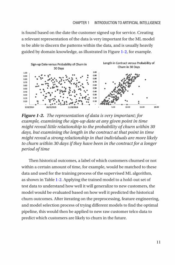
is found based on the date the customer signed up for service. Creating
a relevant representation of the data is very important for the ML model
to be able to discern the patterns within the data, and is usually heavily
guided by domain knowledge, as illustrated in Figure 1-2, for example.
Figure 1-2. The representation of data is very important; for example, examining the sign-up date at any given point in time might reveal little relationship to the probability of churn within 30 days, but examining the length in the contract at that point in time might reveal a strong relationship in that individuals are more likely to churn within 30 days if they have been in the contract for a longer period of time
Then historical outcomes, a label of which customers churned or not
within a certain amount of time, for example, would be matched to these
data and used for the training process of the supervised ML algorithm,
as shown in Table 1-2. Applying the trained model to a hold-out set of
test data to understand how well it will generalize to new customers, the
model would be evaluated based on how well it predicted the historical
churn outcomes. After iterating on the preprocessing, feature engineering,
and model selection process of trying different models to find the optimal
pipeline, this would then be applied to new raw customer telco data to
predict which customers are likely to churn in the future.
Chapter 1 IntroduCtIon to artIfICIal IntellIgenCe

12
This traditional, supervised ML approach as summarized in Figure 1- 3
works for many problems and has been used extensively across many
industries. In operations and workforce management, ML has been used
for predictive maintenance solutions and smart building management, as
well as enhanced supply chain management. For example, Rockwell is able
to save up to $300,000 a day through predictive maintenance solutions that
monitor the health of pumps in offshore rigs (Microsoft, 2015). In marketing
and customer relationship scenarios, ML is used to create personalized
experiences, make product recommendations, and better predict customer
acquisition and churn. In finance, fraud detection solutions and financial
forecasting are often aided by ML-backed solutions.
Table 1-2. Example Output of Simple Feature Engineering and
Matching to the Label of Churn in the Next 30 days
Name Month Total Phone Min Months with Telco Churn Next 30 Days
Mary 2.2011 44 0 0
Mary 3.2011 51 1 0
… … … … …
thomas 6.2013 152 0 0
thomas 7.2013 201 1 0
thomas 8.2013 120 2 1
Note In this case, 0 represents that the individual did not churn, and 1 represents that the individual did churn.
Chapter 1 IntroduCtIon to artIfICIal IntellIgenCe

13
Figure 1-3. Approach for classical, supervised machine learning solutions
Chapter 1 IntroduCtIon to artIfICIal IntellIgenCe
14
Deep LearningAlthough traditional ML approaches work well for many scenarios as
discussed earlier, much of the world is quantized in a representation that
has no easily extractable semantics, such as audio snippets or pixels in
an image.
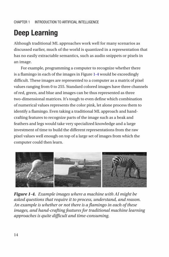
For example, programming a computer to recognize whether there
is a flamingo in each of the images in Figure 1-4 would be exceedingly
difficult. These images are represented to a computer as a matrix of pixel
values ranging from 0 to 255. Standard colored images have three channels
of red, green, and blue and images can be thus represented as three
two-dimensional matrices. It’s tough to even define which combination
of numerical values represents the color pink, let alone process them to
identify a flamingo. Even taking a traditional ML approach and hand-
crafting features to recognize parts of the image such as a beak and
feathers and legs would take very specialized knowledge and a large
investment of time to build the different representations from the raw
pixel values well enough on top of a large set of images from which the
computer could then learn.
Figure 1-4. Example images where a machine with AI might be asked questions that require it to process, understand, and reason. An example is whether or not there is a flamingo in each of these images, and hand-crafting features for traditional machine learning approaches is quite difficult and time-consuming.
Chapter 1 IntroduCtIon to artIfICIal IntellIgenCe
15
Similarly, traditional natural language processing requires complex
and time-consuming task-specific feature engineering. For processing
speech, different languages, intonations, environments, and noise create
subtle differences that make crafting relevant features extremely difficult.
Deep learning, which is the focus of this book, is a further subfield of
AI and ML that has especially shown promise on these types of problems
without easily extractable semantics such as images, audio, and text data
(Goodfellow, Bengio, & Courville, 2016). With deep learning approaches,
a multilayer deep neural network (DNN) model is applied to vast amounts
of data. Deep learning models often have millions of parameters; therefore
they require extremely large training sets to avoid overfitting. The goal of
the model is to map from an input to an output (e.g., pixels in an image to
classification of image as flamingo; audio clip to transcript). The raw input
is processed through a series of functions. The basic idea is that supervised
deep learning models learn the optimal weights of the functions
mapping this input data to the output classification through examining
vast amounts of data and gradually correcting itself as it compares the
predicted result with the ground truth labeled data.
The early variants of these models and concepts dating back to the
1950s were based loosely on ideas on how the human brain might process
information and were called artificial neural networks. The model learns
to process data through learning patterns. First are simple patterns such
as edges and simple shapes, which are then combined to form more
complicated patterns through the many layers of the model. Current
models often include many layers—some variants even boast over a
hundred layers—and hence the terminology deep. The model thus learns
high-level abstractions automatically through the hierarchical nature of
processing information.
Although data still need to be processed and shaped to fit into a deep
learning model, there is no longer a need to hand-craft features, as the
raw input (e.g., pixel values in an image) is fed directly into the model.
The model learns the features (attributes) of the input data automatically.
Chapter 1 IntroduCtIon to artIfICIal IntellIgenCe
16
There is thus no need for features that represent subparts of the pictures,
such as the beak and leg in the flamingo example earlier. Deep learning
approaches show promise for learning patterns in the input data to be
able to classify directly based on the raw input rather than constructing
features manually. Instead, often more time is spent selecting the structure
of the network, also called the network architecture, and tuning the
hyperparameters, the parameters within the model that are set before the
learning process even begins. This has given rise to the idea that network
architecture engineering is the new feature engineering (Merity, 2016).
Deep learning has also shown promise in several areas of ML where
traditional methods also work well, such as forecasting for predicting
future values in a time series and recommendation systems that aim to
predict the preference a user would have for a given item. More details
on specific types of deep learning models as well as recent trends in deep
learning are covered in Chapters 2 and 3, respectively.
Rise of Deep LearningThe basic ideas and algorithms behind deep learning have been around
for decades, but the massive use of deep learning in consumer and
industrial applications has only occurred in the last few years. Two factors
have especially driven the recent growth in AI applications, and especially
deep learning solutions: increased computation power accelerated by
cloud computing and growth in digital data.
Deep learning models require lots of experimentation and often run on
large training data, thus requiring a large amount of computing resources,
especially hardware such as GPUs and FPGAs that are magnitudes more
efficient than traditional CPUs for the computations in a DNN. Cloud
computing—running workloads remotely through the Internet in a data
center with shared resources—opens access to cheaper hardware and
computing power. Resources can be spun up on demand and suspended
Chapter 1 IntroduCtIon to artIfICIal IntellIgenCe
17
when no longer in use to save on cost, without investments in new
hardware.
With the Internet and connected devices, there is an increasing
digitization of our world and massive amounts of data are being collected.
Of course, understanding how to organize and harness this information
is critical to advancing AI applications. One data collection project that
changed AI research was the ImageNet data set, originally published in
2009, which evolved into a yearly competition for AI algorithms, such as
which algorithm could classify the images by objects with the lowest error
rate (Russakovsky et al., 2015). Deep learning has emerged recently as a
powerful technique thanks in large part to the collection of this ImageNet
data set. “Indeed, if the artificial intelligence boom we see today could
be attributed to a single event, it would be the announcement of the 2012
ImageNet challenge results” (Gershgorn, 2017).
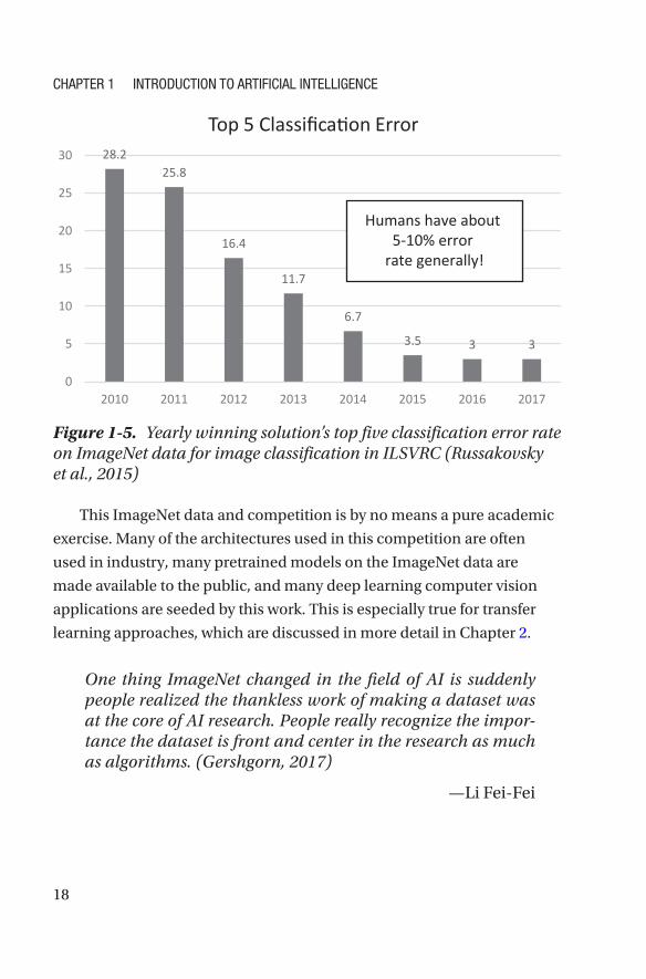
Specifically, in 2012, a deep learning solution drastically improved
over the previous year’s results for classifying objects, as shown in
Figure 1- 5. This solution changed the direction of computer vision
research, and accelerated the research of deep learning in other fields
such as natural language processing and speech recognition. Continuing
more advanced deep learning research, in 2015, Microsoft Research
submitted an entry with an architecture called ResNet with 152 layers
that was the first time an algorithm surpassed human classification
(He, Zhang, Ren, & Sun, 2015).
Chapter 1 IntroduCtIon to artIfICIal IntellIgenCe
18
This ImageNet data and competition is by no means a pure academic
exercise. Many of the architectures used in this competition are often
used in industry, many pretrained models on the ImageNet data are
made available to the public, and many deep learning computer vision
applications are seeded by this work. This is especially true for transfer
learning approaches, which are discussed in more detail in Chapter 2.
One thing ImageNet changed in the field of AI is suddenly people realized the thankless work of making a dataset was at the core of AI research. People really recognize the impor-tance the dataset is front and center in the research as much as algorithms. (Gershgorn, 2017)
—Li Fei-Fei
Figure 1-5. Yearly winning solution’s top five classification error rate on ImageNet data for image classification in ILSVRC (Russakovsky et al., 2015)
Chapter 1 IntroduCtIon to artIfICIal IntellIgenCe

19
Of course, as one might infer from the drastic improvement in the
ImageNet results over the last few years and discussion of the ResNet-152
architecture from Microsoft, there have also been recent advances in
algorithms supporting deep learning solutions and tools available to
create such solutions. Thus, computational power accelerated by cloud
computing, growth in data (especially open labeled data sets), and
advanced algorithms and network architectures have together drastically
changed what is possible with AI in just the last few years.
Not only can deep learning techniques surpass humans in image
recognition, but they are also pushing other areas, such as approaching
human level in speech recognition. In fact, some of the first breakthroughs
in deep learning happened in speech recognition (Dahl, Yu, Deng, &
Acero, 2011). Then in October 2016, Microsoft reached human parity in
the word error rate on the Switchboard data set, a corpus of recorded
telephone conversations used for more than 25 years to benchmark AI
systems (Xiong et al., 2016). These type of innovations are why speech
recognition systems on personal devices and computers have improved so
drastically in the last few years.
Similarly for natural language processing, on January 3, 2018, Microsoft
reached a score of 82.6% on the SQuAD machine reading comprehension
data set comprised of Wikipedia articles. Using these data, the computer
reads a document and answers a question, and was found to outperform
humans on the answers (human performance is at about 82.3%; Linn,
2017; Rajpurkar, Zhang, Lopyrev, & Liang, 2016).
However, it is important to note that these achievements are for a
specific problem or application, and do not represent an AI system that
can generalize to new tasks. It can also be relatively straightforward to
create examples that the computer fails on, so-called adversarial examples
(Jia & Liang, 2017). Additionally, the performance of the system could drop
dramatically even if the original task is modified only slightly. For example,
although computers might now classify general images better than
Chapter 1 IntroduCtIon to artIfICIal IntellIgenCe

20
humans, as shown on ImageNet data discussed earlier, giving open-ended
answers to questions about images is still far from human performance;
there was over 10% difference in accuracy as of June 2017 on the VQA 1.0
data set for visual question answering (AI Index, 2017).
Additionally, deep learning as a general approach still has many
limitations such as the inability to reason and lack of understanding. In
some cases it can also be more difficult to tune deep learning systems
than traditional systems, such as when there is a certain aspect on which
it is not doing well, which in some cases could be easier to account for in
a traditional ML model with fewer parameters. Other ML and AI fields
of research exist and solve other types of problems more accurately than
deep-learning-based approaches. There is also much potential around
the combination of deep learning with other AI research areas such as
reinforcement learning. More details around recent advances, trends, and
limitations are discussed in Chapter 3.
In this book, we focus mainly on deep learning approaches within AI
and applications where intelligent technology can use deep learning to
create solutions that empower people and businesses. These solutions
include enabling better engagement with customers, transformation
of products, and better optimization of operations, for example. Deep
learning applications can often be developed in such a way that they
learn and improve over time as more data are collected and often create
experiences that connect people and technology in more seamless
ways. This book is meant to serve as an introduction to how to develop
deep learning solutions with the Microsoft AI Platform. For a more
comprehensive overview of deep learning in general including more about
the theory and advanced topics, the book by Bengio, Goodfellow, and
Courville (2016) is highly recommended.
Chapter 1 IntroduCtIon to artIfICIal IntellIgenCe

21
Applications of Deep LearningSome classic computer vision problems that can be tackled using deep
learning are shown in Figure 1-6, such as being able to classify images
and find objects within the images. These common technical problems
underlie many different end user applications. For example, photo search
applications such as Microsoft’s Photo App that allow users to type in
descriptions of objects (e.g., “car”) or concepts (e.g., “hug”) and return
relevant results provide a useful capability built through using DNNs.
Figure 1-6. Example computer vision problems
Many deep learning applications for computer vision surround health
care and the medical realm, in subfields where doctors commonly inspect
patients or test results visually, such as in dermatology, radiology, and
ophthalmology. Imagine the possibilities in that a radiologist can inspect
thousands of scans, but a computer can be shown and learn from millions.
Humans globally will benefit from the democratization of these services,
which will over time become even more accurate and efficient. Project
InnerEye is one example, a research project from Microsoft for building
innovative tools for automatic, quantitative analysis of three-dimensional
radiological images to assist expert medical practitioners.
Chapter 1 IntroduCtIon to artIfICIal IntellIgenCe

22
Examples also abound in manufacturing and utilities. Take eSmarts, a
power and utility company based in Norway that provides an automated
energy management system, for example. They use drones to collect
images of power lines and then analyze them using DNNs to automatically
detect faults (Nehme, 2016). Specifically, eSmarts does object detection on
the images to detect discs and then predict whether they are faulty. They
mix real images with synthetic images they have created to create a large
enough data set to be able to predict. Similarly, Jabil, one of the leading
design and manufacturing solution providers, is optimizing manufacturing
operations by analyzing images of their circuit board assembly line to
automatically detect defects (Bunting, 2017). Doing this reduces the
number of boards that have to be manually inspected by the operators
watching the line and increases their throughput.
Analyzing natural language data is another common use of deep
learning. The goal of these applications broadly is for computers to process
natural language, classify text, answer questions, summarize documents,
and translate between languages, for example. Natural language
processing often requires several layers of processing, from the linguistic
level of words and semantics to parts of speech and entities, to the type of
end user applications shown in Figure 1-7 (Goldberg, 2016).
Chapter 1 IntroduCtIon to artIfICIal IntellIgenCe

23
Translating audio data to text is another common application of
deep learning. An example application using deep learning for speech
recognition, Starship Commander is a new virtual reality (VR) game from
Human Interact, where players are active agents in the sci-fi universe
(Microsoft Customer Stories, 2017). Human Interact is building the
lifelike experiences in the game around human speech, allowing users
to influence the storyline and direction of the game through their voice.
To enable this, the game needs to recognize speech and understand the
meaning of that speech based on the users’ underlying intent. Microsoft’s
Custom Speech Service allows developers to build on top of a speech
recognition system that, using deep learning, can overcome obstacles such
as speaking style and background noise. Developers can even train with
a custom script to recognize the key words and phrases from the game to
build a truly custom speech recognition system more quickly and easily
than building from scratch.
Figure 1-7. Example applications of natural language processing from text
Chapter 1 IntroduCtIon to artIfICIal IntellIgenCe

24
This is just the first step of recognizing what words were uttered—the
game then needs to understand what the user means. Imagine the user
is giving a command to start the engine of a ship. There are many ways
someone could give that command. Microsoft’s Language Understanding
Service infers the users’ underlying intent, translating between the speech
recognized by the game and what the user actually means.
The only reason we can build a product like this is because we are building on the deep learning and speech recognition expertise at Microsoft to deliver an entertainment experience that will be revolutionary.
—Alexander Mejia, Owner and Creative Director, Human Interact
Of course, these are just some simple examples that showcase how
deep learning can bring value to business and consumer applications.
Deep learning has shown tremendous potential for applications around
speech, text, vision, forecasting, and recommenders, for example (see
Figure 1-8), and we expect to see tremendous use of deep learning in many
industries and more applications in the future.
Figure 1-8. Example areas where deep learning solutions have demonstrated great performance
Chapter 1 IntroduCtIon to artIfICIal IntellIgenCe

25
Interacting with more applications through speech and text rather than
menus, chatting with bots on a company’s web site or human resources
page to solve routine problems quickly, innovative photo applications that
allow natural search and manipulation, and finding relevant information
quickly from documents are just some example scenarios where deep
learning will drive forward value to businesses and consumers.
SummaryThis chapter introduced the concepts of AI, ML, and deep learning
as summarized in Figure 1-9. Buildingon decades of research and
technological innovations as mentioned briefly in this chapter, Microsoft
now provides services and infrastructure to enable others who want
to build intelligent applications—including powerful deep learning
applications as discussed in this book—through the Microsoft AI Platform
built on the cloud computing platform Azure.
Figure 1-9. Visualization of relationship between artificial intelligence, machine learning, and deep learning
Chapter 1 IntroduCtIon to artIfICIal IntellIgenCe
26
This chapter also discussed reasons behind the recent rise of deep
learning such as increased computational power and increased data set
sizes, especially for labeled data such as ImageNet, which has been made
available publicly. These have propelled forward research in areas such
as computer vision, natural language processing, speech recognition, and
time series analysis. We are also seeing many valuable applications built
on deep learning in areas such as health care, manufacturing, and utilities.
We believe this trend will continue, but that other areas of AI research will
also be useful in the future.
In the next chapter, we introduce common deep learning models and
aspects needed to get started with deep learning. In Chapter 3, we then
discuss some of the emerging trends in deep learning and AI as well as
some of the legal and ethical implications mentioned briefly in this chapter
in more detail.
Chapter 1 IntroduCtIon to artIfICIal IntellIgenCe
27© Mathew Salvaris, Danielle Dean, Wee Hyong Tok 2018 M. Salvaris et al., Deep Learning with Azure, https://doi.org/10.1007/978-1-4842-3679-6_2
CHAPTER 2
Overview of Deep LearningIn Chapter 1, we gave an overview of AI and the basic idea behind deep
learning. We discussed how deep learning—applying artificial neural
network models with a large number of layers—has yielded state-of-the
art results for several research areas, such as image classification, object
detection, speech recognition, and natural language processing.
Deep learning has also shown promise in many applications across
areas such as health care, manufacturing, and retail. In 2017, for example,
an AI system did as well as dermatologists in identifying skin cancer
and a model could diagnose irregular heart rhythms from single-lead
electrocardiogram (ECG) signals better than a cardiologist (Esteva et al.,
2017; Rajpurkar, Hannun, Haghpanahi, Bourn, & Ng, 2017). We believe
this trend will continue: Deep learning will bring value to more scenarios
across many industries and progress toward improved AI experiences will
continue to accelerate.
In this chapter we briefly go over the basics of several types of
networks that are now commonly used. We also describe the data science
workflow for deep learning projects including a description of some of
the popular tools and technologies that data scientists and developers
need to get started when working on a deep learning project. This chapter
also provides practical techniques for getting started with deep learning
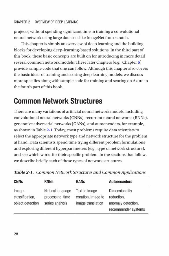
28
projects, without spending significant time in training a convolutional
neural network using large data sets like ImageNet from scratch.
This chapter is simply an overview of deep learning and the building
blocks for developing deep-learning-based solutions. In the third part of
this book, these basic concepts are built on for introducing in more detail
several common network models. These later chapters (e.g., Chapter 6)
provide sample code that one can follow. Although this chapter also covers
the basic ideas of training and scoring deep learning models, we discuss
more specifics along with sample code for training and scoring on Azure in
the fourth part of this book.
Common Network StructuresThere are many variations of artificial neural network models, including
convolutional neural networks (CNNs), recurrent neural networks (RNNs),
generative adversarial networks (GANs), and autoencoders, for example,
as shown in Table 2-1. Today, most problems require data scientists to
select the appropriate network type and network structure for the problem
at hand. Data scientists spend time trying different problem formulations
and exploring different hyperparameters (e.g., type of network structure),
and see which works for their specific problem. In the sections that follow,
we describe briefly each of these types of network structures.
Table 2-1. Common Network Structures and Common Applications
CNNs RNNs GANs Autoencoders
Image
classification,
object detection
Natural language
processing, time
series analysis
Text to image
creation, image to
image translation
Dimensionality
reduction,
anomaly detection,
recommender systems
ChapTer 2 OvervIew Of Deep LearNINg
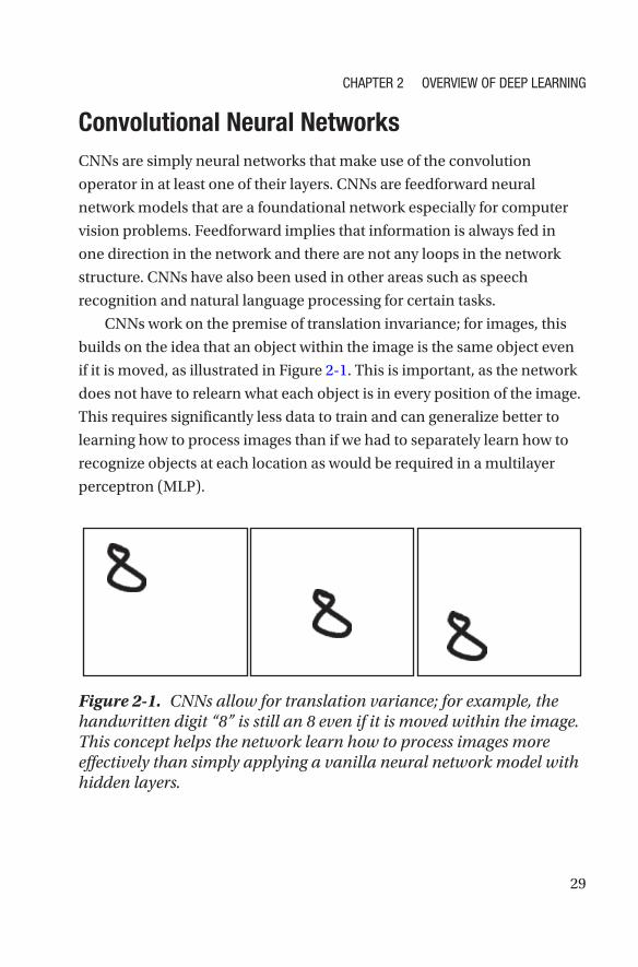
29
Convolutional Neural NetworksCNNs are simply neural networks that make use of the convolution
operator in at least one of their layers. CNNs are feedforward neural
network models that are a foundational network especially for computer
vision problems. Feedforward implies that information is always fed in
one direction in the network and there are not any loops in the network
structure. CNNs have also been used in other areas such as speech
recognition and natural language processing for certain tasks.
CNNs work on the premise of translation invariance; for images, this
builds on the idea that an object within the image is the same object even
if it is moved, as illustrated in Figure 2-1. This is important, as the network
does not have to relearn what each object is in every position of the image.
This requires significantly less data to train and can generalize better to
learning how to process images than if we had to separately learn how to
recognize objects at each location as would be required in a multilayer
perceptron (MLP).
Figure 2-1. CNNs allow for translation variance; for example, the handwritten digit “8” is still an 8 even if it is moved within the image. This concept helps the network learn how to process images more effectively than simply applying a vanilla neural network model with hidden layers.
ChapTer 2 OvervIew Of Deep LearNINg

30
For example, if we want the model to be able to learn to identify what
is a cat, no matter where the cat is located in the image it shares the same
characteristics from which the model should learn: how to identify fur, cat
ears, tail, and so on.
In CNNs, the input image is fed through what is often called a filter or
kernel, which acts as a feature detector in the network. You can think of
these feature detectors as trying to learn aspects such as edges, shapes, or
patterns within the image. This is done by applying the feature detector
on one patch of the image at a time through sliding windows, with the
results of this convolution operation saved into what is called a convolved
image or feature map. CNNs hold the property of translation invariance as
mentioned earlier, as the filters share the same weights as applied to each
image patch that after applying form the convolved image. The depth of
a convolutional layer in a neural network corresponds to the number of
filters used in that layer.
A form of down-sampling through the use of pooling layers is used
to reduce the size of the data going through and remove the potentially
redundant aspects that the network at that stage has learned to react to.
A “max pooling” layer for example simply takes the maximum value from
the output of the convolved image for each window of the image as shown
in Figure 2-2, where the stride represents the number of pixels by which
the window jumps. Convolution and pooling layers are used in many
combinations, transforming an input image into an array that is then input
into at least one fully connected layer that feeds out to the predicted output
classes as visualized in Figure 2-3. The fully connected layers simply act as
a classifier to predict the output class.
ChapTer 2 OvervIew Of Deep LearNINg

31
In other words, CNNs can be conceptually split into two main pieces,
both of which are optimized together:
1. The automatic feature extractor creates the hidden
feature state—features that represent aspects of
image that are relevant for classification—and is
made up of layers such as convolutional and pooling
layers.
2. The classifier is a fully connected neural network
made up of at least one layer that classifies the
hidden feature state.
The automatic feature extractor part of CNN enables the network to
learn aspects such as edges and shapes of the image without having to
explicitly program the network to compute these features as was done with
the use of algorithms such as scale-invariant feature transform (SIFT).
Figure 2-2. Max pooling operation with 2 by 2 filters with stride of two
ChapTer 2 OvervIew Of Deep LearNINg
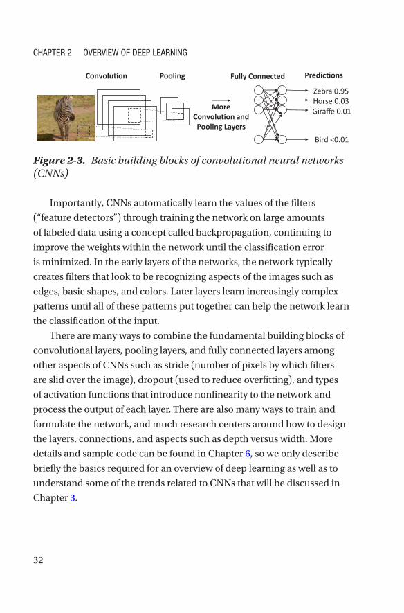
32
Importantly, CNNs automatically learn the values of the filters
(“feature detectors”) through training the network on large amounts
of labeled data using a concept called backpropagation, continuing to
improve the weights within the network until the classification error
is minimized. In the early layers of the networks, the network typically
creates filters that look to be recognizing aspects of the images such as
edges, basic shapes, and colors. Later layers learn increasingly complex
patterns until all of these patterns put together can help the network learn
the classification of the input.
There are many ways to combine the fundamental building blocks of
convolutional layers, pooling layers, and fully connected layers among
other aspects of CNNs such as stride (number of pixels by which filters
are slid over the image), dropout (used to reduce overfitting), and types
of activation functions that introduce nonlinearity to the network and
process the output of each layer. There are also many ways to train and
formulate the network, and much research centers around how to design
the layers, connections, and aspects such as depth versus width. More
details and sample code can be found in Chapter 6, so we only describe
briefly the basics required for an overview of deep learning as well as to
understand some of the trends related to CNNs that will be discussed in
Chapter 3.
Figure 2-3. Basic building blocks of convolutional neural networks (CNNs)
ChapTer 2 OvervIew Of Deep LearNINg

33
Recurrent Neural NetworksRNNs directly make use of sequential information. Sequences passed
to the network could be in the input, output, or even both. The RNN
processes sequences of data through what is sometimes called a “state” or
“memory.” Unlike CNNs, which are feedforward networks, RNNs contain
loops in the network structure, as illustrated in Figure 2-4 and Figure 2-5.
However, note that CNNs have increasingly been shown to be useful for
analyzing sequential information as well, as is mentioned in more detail
in Chapter 7.
Figure 2-4. Recurrent neural networks have a loop in the network structure and process data over sequences
Figure 2-5. RNNs process information over sequences. Often this sequence represents information over time, such that a loop in the RNN can be “unrolled” to see that the output at a given point in time is a function of the inputs at previous points in time.
ChapTer 2 OvervIew Of Deep LearNINg
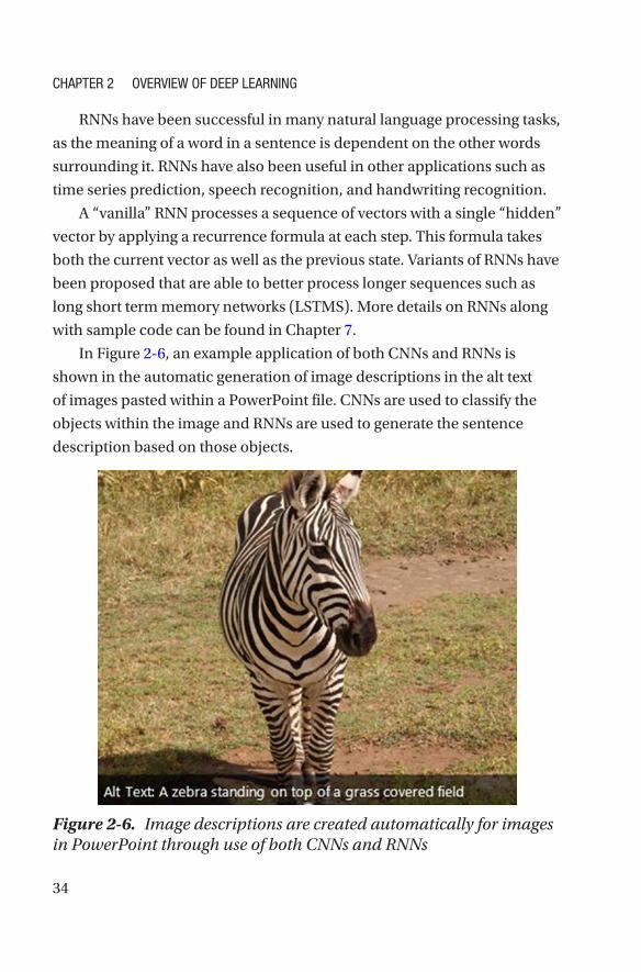
34
RNNs have been successful in many natural language processing tasks,
as the meaning of a word in a sentence is dependent on the other words
surrounding it. RNNs have also been useful in other applications such as
time series prediction, speech recognition, and handwriting recognition.
A “vanilla” RNN processes a sequence of vectors with a single “hidden”
vector by applying a recurrence formula at each step. This formula takes
both the current vector as well as the previous state. Variants of RNNs have
been proposed that are able to better process longer sequences such as
long short term memory networks (LSTMS). More details on RNNs along
with sample code can be found in Chapter 7.
In Figure 2-6, an example application of both CNNs and RNNs is
shown in the automatic generation of image descriptions in the alt text
of images pasted within a PowerPoint file. CNNs are used to classify the
objects within the image and RNNs are used to generate the sentence
description based on those objects.
Figure 2-6. Image descriptions are created automatically for images in PowerPoint through use of both CNNs and RNNs
ChapTer 2 OvervIew Of Deep LearNINg
35
Generative Adversarial NetworksGANs are a more recent development in deep learning that actually
solves a given problem through training two separate network models
in competition with each other (Goodfellow et al., 2014). In recent years,
GANs have shown tremendous potential and have been applied in
various scenarios, ranging from image synthesis, enhancing the quality
of images (superresolution), image-to-image translations, to text-to-
image generation, and more. In addition, GANs are the building blocks
for advancements in the use of AI for art, music, and creativity (e.g., music
generation, music accompaniment, poetry generation, etc.).
GANs are emerging as powerful techniques for both unsupervised and
semisupervised learning. A basic GAN consists of the following:
• A generative model (i.e., generator) generates an
object. The generator does not know anything about
the real objects and learns by interacting with the
discriminator. For example, a generator can generate
an image.
• A discriminative model (i.e., discriminator)
determines whether an object is real (usually
represented by a value close to 1) or fake (represented
by a value close to 0).
• An adversarial loss (or error signal) is provided by
the discriminator to the generator such that it enables
the generator to generate objects that are as close as
possible to the real objects.
More details about GANs are included along with sample code
Chapter 8.
ChapTer 2 OvervIew Of Deep LearNINg
36
We expect that GANs will become more popular in the coming years,
even outside of the use of creative applications, as they have potential to
address how to create unsupervised learning methods that would greatly
expand the reach of ML applications. Today, these types of models take
a long time to train and are notoriously difficult to tune, and we expect
that research will continue to advance the practicality of these networks
for real applications. As this type of technology sees more real-world
applications, improves on quality, and expands to more mediums such as
videos, we believe more debate will surface over their use. For example,
the implications of not being able to discern true content from fake are
quite far-reaching, with examples already highlighted in the media such
as near-realistic fake words inserted into videos of politicians speaking
(Metz & Collins, 2018).
AutoencodersAutoencoders are another type of a feedforward network and have
been used for applications such as dimensionality reduction, anomaly
detection, and learning generative models. These neural network models
have an input layer, an output layer, and at least one hidden layer in
between. Importantly, autoencoders have the same number of units in
the input layer as the output layer, and their purpose is thus to reconstruct
the original values in the input layer. Of course, these are designed in
such a way that they do not copy the input data exactly but are restricted
so that they can only learn approximately, such as having a smaller
dimension than the input data, as one example. Autoencoders thus learn
most relevant properties to reconstruct the input data. As such, they
can be useful for unsupervised learning applications where there is no
target value for prediction or for learning features for input into another
algorithm. They have shown promise for many applications such as
recommender systems (Kuchaiev & Ginsburg, 2017).
ChapTer 2 OvervIew Of Deep LearNINg
37
Deep Learning WorkflowFor many AI projects, deep learning techniques are often used as the
building block for building innovative solutions ranging from image
classification and object detection to image segmentation, image
similarity, and text analytics (e.g., sentiment analysis, key phrase
extraction). Often, people will ask, “How do I get started with using deep
learning in my team?” To get started with deep learning, it is important
to understand the tools and technologies that are used in deep learning
projects and the workflow for building a solution.
Given the business requirements for an innovative solution, a data
scientist will need to map it to one or more deep learning tasks. For
example, let’s say a retail business wants to create an end-to-end customer
shopping experience for mobile devices, where customers can take a
photo of a shirt or a dress, and an application running on the mobile
device can then match it to the shirts and dresses in the shopping catalog.
To achieve this, the data scientist maps this to an image similarity problem:
Take a new input image, and match it against all the shirts and dresses in
the catalog. The top N images will be returned to the mobile application.
While working with the application developers, other requirements need
to be addressed as well, like identifying and cropping the image to just the
person wearing the shirt or dress, for example. This will require the use of
both object detection and image classification.
Once the deep learning task is identified, a typical deep learning
workflow will include the following:
1. Identify relevant data set(s).
2. Preprocess the data set.
3. Train the model.
4. Check the performance of the model.
ChapTer 2 OvervIew Of Deep LearNINg

38
5. Tune the model.
6. Deploy the model.
7. Iterate and collect more data to enable retraining.
Finding Relevant Data Set(s)Most companies wanting to get started with deep learning projects often
face difficultly when trying to find relevant data set(s) that they can use
for training their deep learning models for a specific business scenario.
In addition, the data set needs to be labeled. For example, to train a CNN
to identify the type of clothing (e.g., polo shirt, t-shirt, dress, jeans), a data
set consisting of images of clothing, with labels denoting whether the
image is a shirt, dress, t-shirt, or jeans is required. These images can come
from the existing product catalogs, public image data sets (e.g., diverse set
of images from ImageNet, CIFAR-10, Deep Fashion), and scraped from
various web sites.
To seed the initial training and validation data set if data are not
already available, data scientists often use a search engine (Figure 2-7)
for performing an image search on a specific class (e.g., jeans), where the
image owner has labeled the image as free to use for commercial use.
ChapTer 2 OvervIew Of Deep LearNINg
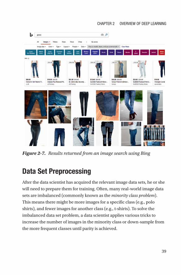
39
Data Set PreprocessingAfter the data scientist has acquired the relevant image data sets, he or she
will need to prepare them for training. Often, many real-world image data
sets are imbalanced (commonly known as the minority class problem).
This means there might be more images for a specific class (e.g., polo
shirts), and fewer images for another class (e.g., t-shirts). To solve the
imbalanced data set problem, a data scientist applies various tricks to
increase the number of images in the minority class or down-sample from
the more frequent classes until parity is achieved.
Figure 2-7. Results returned from an image search using Bing
ChapTer 2 OvervIew Of Deep LearNINg
40
Another commonly used preprocessing technique is data augmentation
to help the model generalize over multiple conditions, to improve its
invariance to aspects such as rotation, translation, and scaling. This
includes applying various transformation to the image, such as scaling,
rotating, random cropping of the image, flipping the image, adjusting the
brightness and contrast, and more. Various data augmentation capabilities
are supported in the different deep learning frameworks.
Training the ModelAfter the data set has been preprocessed and prepared, the data scientist is
ready to start designing the deep learning model architecture and training
the model. The key ingredients that enable effective modeling and training
of deep learning models are (1) choosing a deep learning toolkit, and (2)
training using hardware such as GPUs. This is discussed in more detail in
the next section in this chapter.
Depending on the size of the data set, the model can be trained on a
local machine (e.g., laptop, PC, Mac) or using infrastructure available in
the public cloud, such as Microsoft Azure. Azure provides both NC-series
virtual machines (VM) with Nvidia GPUs, as well as a managed service,
called Azure Batch AI, which enable you to easily scale up and down GPUs
that you need for your deep learning jobs. This will be covered in more
detail in Chapters 4 and 9.
Validating and Tuning the ModelDuring training of the deep neural network, there are several key metrics
that will provide insights on the learning efficiency and the quality of the
models at each epoch. An epoch refers to a full pass of the training data set.
Two metrics are commonly tracked: (1) loss function, and (2) training and
validation accuracy.
ChapTer 2 OvervIew Of Deep LearNINg
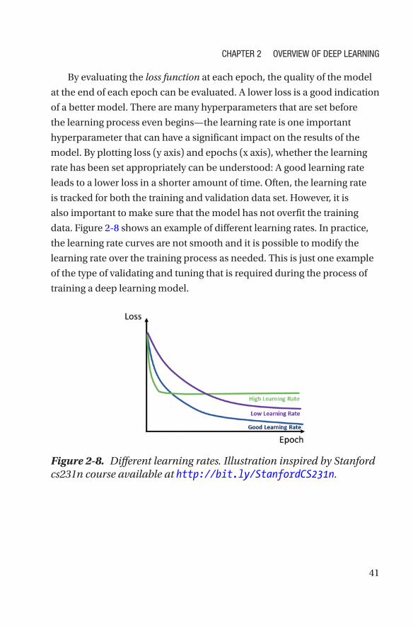
41
By evaluating the loss function at each epoch, the quality of the model
at the end of each epoch can be evaluated. A lower loss is a good indication
of a better model. There are many hyperparameters that are set before
the learning process even begins—the learning rate is one important
hyperparameter that can have a significant impact on the results of the
model. By plotting loss (y axis) and epochs (x axis), whether the learning
rate has been set appropriately can be understood: A good learning rate
leads to a lower loss in a shorter amount of time. Often, the learning rate
is tracked for both the training and validation data set. However, it is
also important to make sure that the model has not overfit the training
data. Figure 2-8 shows an example of different learning rates. In practice,
the learning rate curves are not smooth and it is possible to modify the
learning rate over the training process as needed. This is just one example
of the type of validating and tuning that is required during the process of
training a deep learning model.
Figure 2-8. Different learning rates. Illustration inspired by Stanford cs231n course available at http://bit.ly/StanfordCS231n.
ChapTer 2 OvervIew Of Deep LearNINg
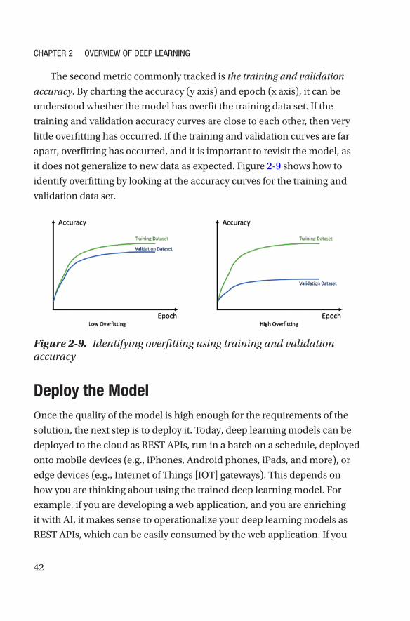
42
The second metric commonly tracked is the training and validation
accuracy. By charting the accuracy (y axis) and epoch (x axis), it can be
understood whether the model has overfit the training data set. If the
training and validation accuracy curves are close to each other, then very
little overfitting has occurred. If the training and validation curves are far
apart, overfitting has occurred, and it is important to revisit the model, as
it does not generalize to new data as expected. Figure 2-9 shows how to
identify overfitting by looking at the accuracy curves for the training and
validation data set.
Figure 2-9. Identifying overfitting using training and validation accuracy
Deploy the ModelOnce the quality of the model is high enough for the requirements of the
solution, the next step is to deploy it. Today, deep learning models can be
deployed to the cloud as REST APIs, run in a batch on a schedule, deployed
onto mobile devices (e.g., iPhones, Android phones, iPads, and more), or
edge devices (e.g., Internet of Things [IOT] gateways). This depends on
how you are thinking about using the trained deep learning model. For
example, if you are developing a web application, and you are enriching
it with AI, it makes sense to operationalize your deep learning models as
REST APIs, which can be easily consumed by the web application. If you
ChapTer 2 OvervIew Of Deep LearNINg

43
are developing a mobile application, you should consider both connected
and disconnected scenarios, as well as latency requirements. You will
either have the models running offline on the mobile device, or a hybrid
model where you have both combinations of models that run on device
and REST APIs that provide more powerful functionality in the cloud.
To deploy the deep learning models as REST APIs, several options
exist. You can leverage Azure Machine Learning Operationalization
services (more details will be covered in subsequent chapters in the book)
to host the model in a docker container, and expose one or more REST
endpoints, or you can build your own hosting stack (e.g., use of Flask,
CherryPy backed by high-performing web server like NGINX). You can
easily deploy this hosting stack on Microsoft Azure, as well. Depending on
the scenario, you might want to run the model in batch mode on a large set
of data on a schedule. The type of hardware such as GPUs is also a relevant
factor to consider. More details are discussed in Chapter 10.
For more consideration around approaching data science workflows
in general, including deep learning projects, we suggest the Microsoft
Team Data Science Process available at http://bit.ly/MSFT_TDSP.
This includes an overview of the data science life cycle, a suggested
standardized project structure and infrastructure, and resources for data
science projects.
Deep Learning Frameworks & ComputeAs mentioned earlier, two key ingredients you need for performing
deep learning training are (1) use of a deep learning framework, and
(2) performing training using a GPU. General-purpose computing on
GPUs especially through efficient use of matrix multiplication has been
accelerated through frameworks such as CUDA and OpenCL. These have
enabled higher level libraries such as cuDNN on top of CUDA for building
deep neural nets; cuDNN underpins popular deep learning libraries.
ChapTer 2 OvervIew Of Deep LearNINg
44
There are now many popular deep learning frameworks such as
Tensorflow, PyTorch, CNTK, MXNet, and Caffe2, as well as popular higher
level APIs such as Keras and Gluon. The choice of a deep learning toolkit
depends on many factors, including the availability of good tutorials
and existing implementations of model architectures and pretrained
models, skill sets of the AI talents in the company, flexibility of the toolkit
in expressing complex deep neural networks, availability of built-in
helper functionalities (e.g., rich set of APIs for data augmentation and
transformation), ability to effectively leverage both CPUs and GPUs, and
ability to perform distributed training.
We recommend the deep learning comparison repo available at
http://bit.ly/DLComparisons for understanding differences between
different deep learning frameworks on a few common scenarios, with
example frameworks considered as illustrated in Figure 2-10. This repo has
several stated goals:
1. A “Rosetta Stone” of deep learning frameworks to
allow data scientists to easily leverage their expertise
from one framework to another.
2. Optimized GPU code using the most up-to-date
highest level APIs.
3. A common setup for comparisons across GPUs
(potentially CUDA versions and precision).
4. A common setup for comparisons across languages
(Python, Julia, R).
5. The possibility to verify expected performance of
own installation.
6. Collaboration between different open source
communities.
ChapTer 2 OvervIew Of Deep LearNINg
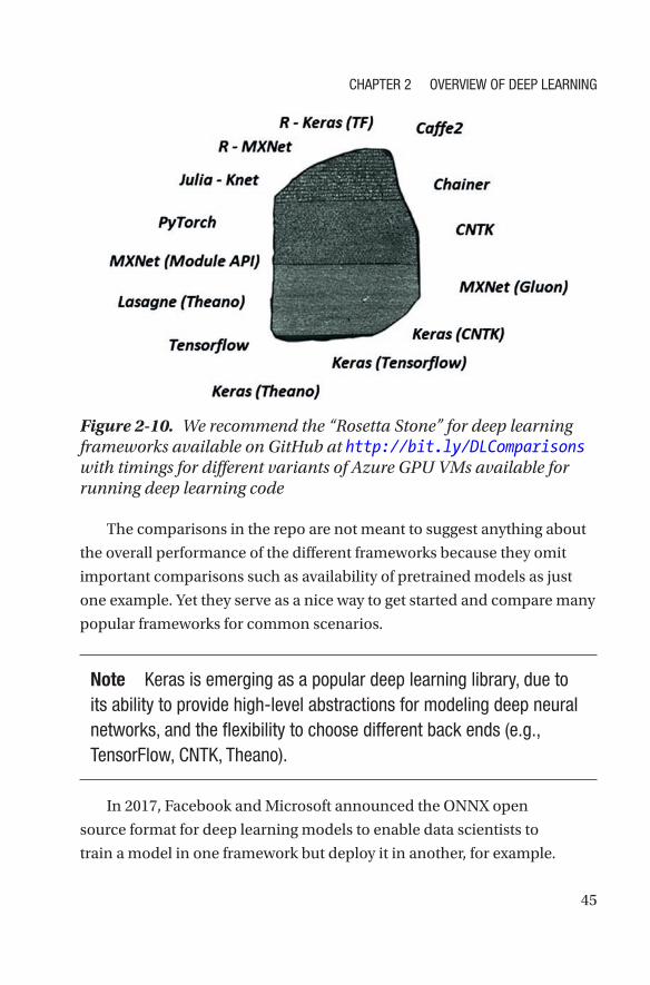
45
The comparisons in the repo are not meant to suggest anything about
the overall performance of the different frameworks because they omit
important comparisons such as availability of pretrained models as just
one example. Yet they serve as a nice way to get started and compare many
popular frameworks for common scenarios.
Note Keras is emerging as a popular deep learning library, due to its ability to provide high-level abstractions for modeling deep neural networks, and the flexibility to choose different back ends (e.g., Tensorflow, CNTK, Theano).
In 2017, Facebook and Microsoft announced the ONNX open
source format for deep learning models to enable data scientists to
train a model in one framework but deploy it in another, for example.
Figure 2-10. We recommend the “Rosetta Stone” for deep learning frameworks available on GitHub at http://bit.ly/DLComparisons with timings for different variants of Azure GPU VMs available for running deep learning code
ChapTer 2 OvervIew Of Deep LearNINg
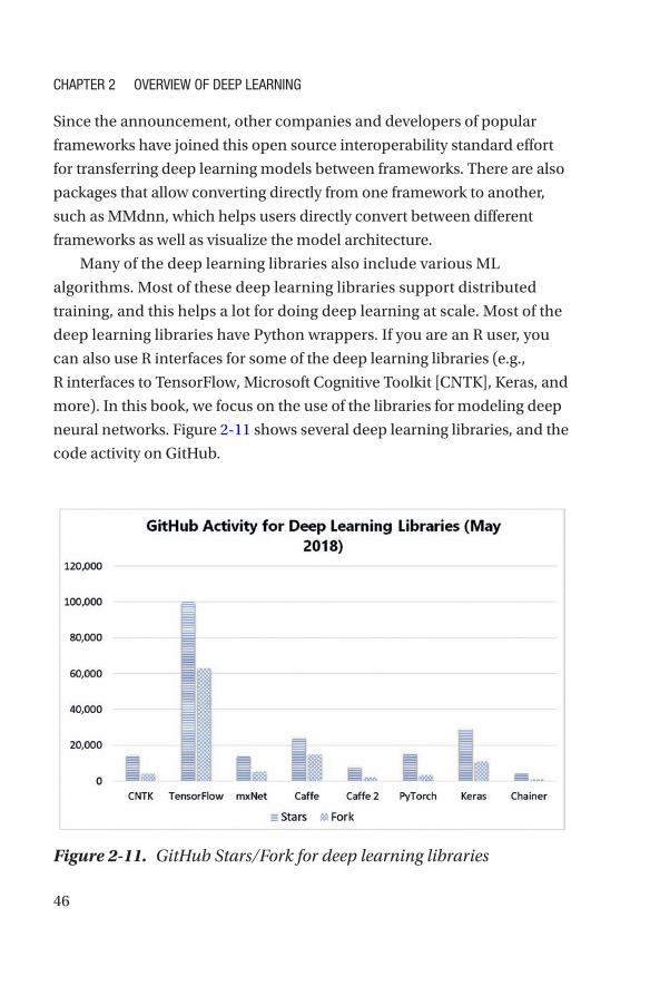
46
Since the announcement, other companies and developers of popular
frameworks have joined this open source interoperability standard effort
for transferring deep learning models between frameworks. There are also
packages that allow converting directly from one framework to another,
such as MMdnn, which helps users directly convert between different
frameworks as well as visualize the model architecture.
Many of the deep learning libraries also include various ML
algorithms. Most of these deep learning libraries support distributed
training, and this helps a lot for doing deep learning at scale. Most of the
deep learning libraries have Python wrappers. If you are an R user, you
can also use R interfaces for some of the deep learning libraries (e.g.,
R interfaces to TensorFlow, Microsoft Cognitive Toolkit [CNTK], Keras, and
more). In this book, we focus on the use of the libraries for modeling deep
neural networks. Figure 2-11 shows several deep learning libraries, and the
code activity on GitHub.
Figure 2-11. GitHub Stars/Fork for deep learning libraries
ChapTer 2 OvervIew Of Deep LearNINg
47
Although most of the examples in this book use Tensorflow, the
Microsoft AI Platform supports any open source framework. In addition,
we include a few examples of using other frameworks, such as a
pedagogical example showing how one can train a CNN model using
many different deep learning frameworks using the Microsoft Batch AI
service in Chapter 9.
GPUs make the training of deep learning models possible within a
reasonable time frame. In recent years, innovations in both algorithms and
availability of faster GPUs have enabled the training of deep learning models
to be completed quickly. For example, the training of CNNs like ResNet-50
using the publicly available ImageNet data set used to take 14 days or more
before 2017. Within months in 2017, the time taken to train ResNet-50
decreased significantly, from an hour to approximately 15 minutes. Preferred
Network was able to train ResNet-50 CNN model with ChainerMN with
1,024 P100 GPUs in 15 minutes in November 2017, for example.
Jump Start Deep Learning: Transfer Learning and Domain AdaptationA major trend to jump starting deep learning solutions has been to build
prior knowledge into the development of the model so it does not learn
solely from the data of the problem at hand. Two common ways this is
done is through a concept called transfer learning in computer vision and
domain adaptation mainly through the use of word embeddings in natural
language processing.
Transfer learning is especially useful in computer vision tasks such as
image classification and object detection. The basic idea is that we want to
be able to transfer our learning from one application to another. Transfer
learning enables data scientists to quickly adapt existing pretrained
models (e.g., AlexNet, ResNet-50, InceptionV3, etc.) to new domains.
For example, a CNN can be trained on the large ImageNet data with
ChapTer 2 OvervIew Of Deep LearNINg
48
millions of examples. This CNN then internally holds the representation
of how to process images well, such as how to detect edges, shapes, and
patterns to distinguish between objects. We thus want to be able to use
this knowledge, captured within the weights of the network to use in a
classification scenario with significantly less data, such as distinguishing
between types of shirts on a retail web site or distinguishing between
defects and nondefects through images taken on a manufacturing
assembly line, for example.
Thus to jump start deep learning projects in computer vision, for
example, we recommend data scientists leverage pretrained models that
are trained using publicly available data sets such as ImageNet, CIFAR-10,
and COCO. These data sets contain millions of images (from diverse
domains) and have been carefully curated by the respective research labs
(often through crowd-sourcing efforts) and annotated with class labels.
The pretrained models are used to jump start image classification,
object detection, and image segmentation problems. These pretrained
models, trained on large image data sets, are used either as featurizers for
new images, or to further fine-tune to adapt to domain-specific images
(e.g., medical x-ray images, PCB circuit board images, etc.) to improve
on the quality of the predictions. Table 2-2 shows the different types of
transfer learning. Table 2-3 shows the input and output initialization
required for each type of transfer learning.
ChapTer 2 OvervIew Of Deep LearNINg
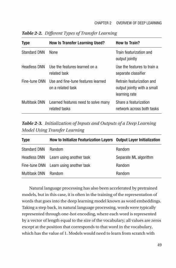
49
Table 2-3. Initialization of Inputs and Outputs of a Deep Learning
Model Using Transfer Learning
Type How to Initialize Featurization Layers Output Layer Initialization
Standard DNN random random
headless DNN Learn using another task Separate ML algorithm
fine-tune DNN Learn using another task random
Multitask DNN random random
Table 2-2. Different Types of Transfer Learning
Type How Is Transfer Learning Used? How to Train?
Standard DNN None Train featurization and
output jointly
headless DNN Use the features learned on a
related task
Use the features to train a
separate classifier
fine-tune DNN Use and fine-tune features learned
on a related task
retrain featurization and
output jointly with a small
learning rate
Multitask DNN Learned features need to solve many
related tasks
Share a featurization
network across both tasks
Natural language processing has also been accelerated by pretrained
models, but in this case, it is often in the training of the representation of
words that goes into the deep learning model known as word embeddings.
Taking a step back, in natural language processing, words were typically
represented through one-hot encoding, where each word is represented
by a vector of length equal to the size of the vocabulary; all values are zeros
except at the position that corresponds to that word in the vocabulary,
which has the value of 1. Models would need to learn from scratch with
ChapTer 2 OvervIew Of Deep LearNINg
50
just the data of the problem at hand every time to understand how to
process the words and what their meaning was in the context of the
specific natural language processing task. In contrast, word embeddings
are low-dimensional vectors that encode semantic meaning of words,
encoding semantically related words close to each other in the embedding
vector space.
Importantly, word embeddings can be trained on large, unlabeled data
and many pretrained word embeddings are made available for use in other
natural language processing tasks. By using a pretrained word embedding
such as one trained on Google News, knowledge about how words are
related to each other is embedded into the model built with them.
Word embedding vectors are learned using so-called word2vec
algorithms such as Skip-Gram and CBOW. These are simple neural
network models that aim to predict words in a window around each
word. The concept is that semantically related words will appear in
similar context and thus obtain similar vector representations. Of course,
domain-specific word embeddings might be beneficial to better represent
words within the model, and recent research has also focused on how
to allow better domain adaptation between natural language processing
applications.
Models LibraryMany pretrained deep neural networks are available for each of the deep
learning libraries. For example, Microsoft CNTK and TensorFlow provide
pretrained models for several state-of-the-art CNNs (AlexNet, GoogLeNet,
ResNet, and VGG). Caffe’s Model Zoo provides a rich set of 40 and more
pretrained models for state-of-the-art CNN (ResNet, Inception, VGG,
etc.), and supporting various scenarios (e.g., car model identification,
recognizing different landmarks and places, scene recognition, etc.).
Google Word2Vec is a popular pretrained word-embedding model with
many available tutorials.
ChapTer 2 OvervIew Of Deep LearNINg

51
You can use these pretrained models to jump start your deep learning
projects, or further fine-tune the network for your business scenarios. This
will often save significant amounts of time training the base models on a
diverse data set.
More Info find out more about example pretrained models:
CNTK pretrained Image Model: http://bit.ly/CNTKModelsTensorflow Official Model: http://bit.ly/TensorflowModelsCaffe Model Zoo: http://bit.ly/CaffeModelsTensorflow word2vec: http://bit.ly/TensorflowWord2Vec
SummaryThis chapter briefly introduced several common types of neural networks
including CNNs, RNNs, and GANs, which are discussed in more detail
along with sample code in later chapters. We also discussed the deep
learning workflow, the nuts and bolts of starting a deep learning project
and some of the libraries that can be used to develop and train deep
neural networks. To help jump start deep learning projects, data scientists
and developers can leverage pretrained models as the foundations for
featurizing images or use them to further customize and fine-tune to adapt
for your business domains. In the next chapter, we discuss some of the
trends in the deep learning field as well as some of the limitations of this
type of modeling approach.
ChapTer 2 OvervIew Of Deep LearNINg

53© Mathew Salvaris, Danielle Dean, Wee Hyong Tok 2018 M. Salvaris et al., Deep Learning with Azure, https://doi.org/10.1007/978-1-4842-3679-6_3
CHAPTER 3
Trends in Deep LearningThis chapter discusses some of the trends in deep learning and related
fields. We cover specifically which trends might be useful for what tasks as
well as discuss some of the methods and ideas that could have far-reaching
implications but have yet to be applied to many real-world problems. We
finish by covering briefly some of the current limitations of deep learning
as well as some other areas of AI that seem to hold promise for future AI
applications, and discuss briefly some of the ethical and legal implications
of deep learning applications.
Variations on Network ArchitecturesOne of the first trends in the field of deep learning was to build deeper
networks with more layers to solve problems with increasing complexity.
However, training such deep networks is difficult, as they are harder to
optimize, and accuracy can degrade rather than improve. As mentioned
in Chapter 1, Microsoft released a network structure in 2015 that builds on
the concept of residual learning with their architecture called ResNet (He,
Zhang, Ren, & Sun, 2015). Instead of trying to learn a direct mapping of the
underlying relationship between an input and output within the network,
the difference or residual between the two is learned. With this concept,
54
training of networks substantially deeper than previously used before
became possible, with a network of 152 layers winning the 2015 ILSVRC
competition on the ImageNet data. A class of networks called Inception
networks alternatively focus on wide architectures where not all layers are
simply stacked sequentially, aiming to increase both performance as well as
computational efficiency of neural network models (Szegedy, Liu, et al., 2014).
Note To accelerate development, practitioners should leverage network architectures from the research community such as Resnet-152 rather than trying to build and train CNNs from scratch.
Residual Networks and Variants There have been many suggested network architectures in recent years,
and this trend continues to result in more network architecture choices.
Many architectures rely on modifications to ResNets, such as ResNeXt,
MultiResNet, and PolyNet (Abdi & Nahavandi, 2017; Xie, Girshick, Dollár,
Zhuowen, & He, 2017; Zhang, Li, Loy, & Lin, 2017). Combining different
types of approaches has also been considered such as Inception-ResNet
(Szegedy, Ioffe, & Vanhoucke, 2016). In contrast, FractalNet is an extremely
deep architecture that does not rely on residuals (Larsson, Maire, &
Shakhnarovi, 2017).
DenseNet DenseNet is another popular network structure where each layer
is connected to all other layers; its popularity lies in that it allows a
substantial reduction in the number of parameters through feature reuse
while alleviating a problem related to training of the networks called
vanishing gradients (G. Huang, Liu, van der Maaten, & Weinberger, 2018).
ChapTeR 3 TReNds iN deep LeaRNiNg
55
Small Models, Fewer Parameters Related to the reduction of the number of parameters with DenseNet,
another trend in CNNs is for the creation of more efficient networks that
are built on fewer parameters and have a smaller model size. In general,
larger networks enable more accurate predictions, but there are clever
ways of creating architectures and conducting model compression
to achieve performance close to or at par with larger networks. These
networks can thus be run faster and with less processing power, which can
be especially useful, for example, on embedded and mobile devices where
the computational power and storage are limited.
SqueezeNet, introduced by Iandola et al. (2016), is described as
having accuracy similar to AlexNet with 50 times fewer parameters and
model size less than 0.5 MB, using depth-wise separable convolutions
to reduce the number of parameters. MobileNet is another example
that was designed specifically for mobile and embedded vision
applications (Howard et al., 2017), which has recently been extended
with MobileNetV2. Besides designing efficient smaller networks,
alternatives include pruning weights from existing deep networks,
pruning filters, and quantizing weights within the network (Mittal,
Bhardwaj, Khapra, & Ravindran, 2018). As one example, by pruning
certain connections in the VGG16 architecture, the size can be reduced
by a factor of 49 without modifying the predictions from the model
(Han, Mao, & Dally, 2016).
In practice, we recommend data scientists try many network
structures based on the current research that are often made available
through model zoos and different deep learning frameworks as was
described Chapter 2. Data scientists must try the different options and
consider the trade-offs between aspects such as ease of training and
speed of scoring the models as required for the specific data set and
problem at hand.
ChapTeR 3 TReNds iN deep LeaRNiNg
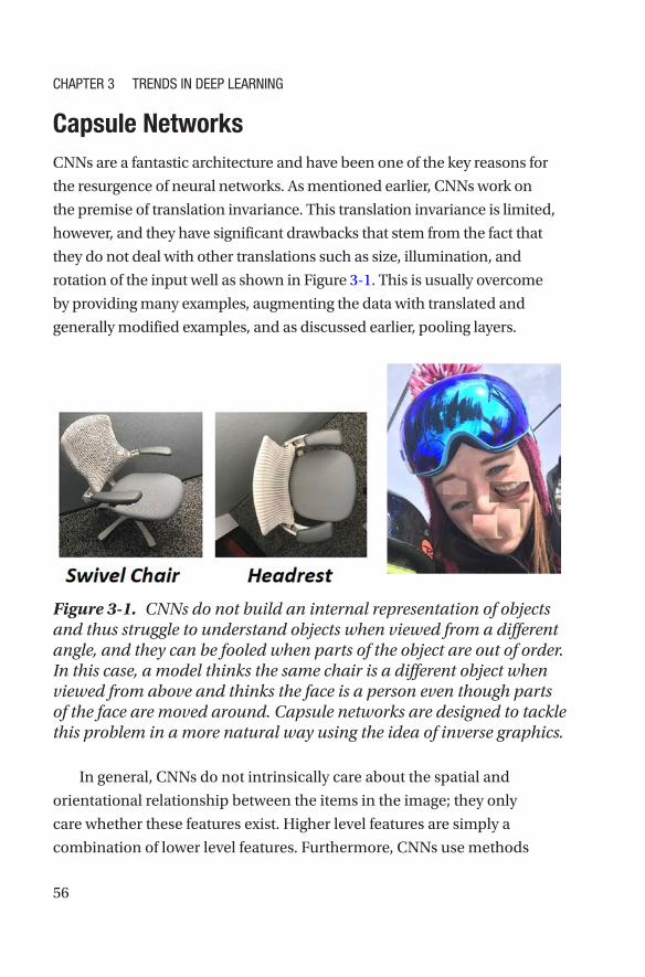
56
Capsule NetworksCNNs are a fantastic architecture and have been one of the key reasons for
the resurgence of neural networks. As mentioned earlier, CNNs work on
the premise of translation invariance. This translation invariance is limited,
however, and they have significant drawbacks that stem from the fact that
they do not deal with other translations such as size, illumination, and
rotation of the input well as shown in Figure 3-1. This is usually overcome
by providing many examples, augmenting the data with translated and
generally modified examples, and as discussed earlier, pooling layers.
Figure 3-1. CNNs do not build an internal representation of objects and thus struggle to understand objects when viewed from a different angle, and they can be fooled when parts of the object are out of order. In this case, a model thinks the same chair is a different object when viewed from above and thinks the face is a person even though parts of the face are moved around. Capsule networks are designed to tackle this problem in a more natural way using the idea of inverse graphics.
In general, CNNs do not intrinsically care about the spatial and
orientational relationship between the items in the image; they only
care whether these features exist. Higher level features are simply a
combination of lower level features. Furthermore, CNNs use methods
ChapTeR 3 TReNds iN deep LeaRNiNg

57
that reduce the spatial dimensions of the data and in effect increase the
receptive field, the field of view of the higher level nodes. This allows the
nodes to detect higher level features in larger regions of the input image.
One of the methods of doing this is max pooling, which we explained in
Chapter 2. By using max pooling, though, the CNNs lose spatially acuity.
For this reason, max pooling is viewed as a bit of an anathema by Hinton
and therefore he sought to devise a new architecture, capsule networks
(Sabour, Frosst, & Hinton, 2017).
Capsule networks are inspired by the idea of inverse graphics. In
traditional graphics we describe an object and its pose parameters and
through the process of rendering, the object is displayed on a screen. In
inverse graphics we want to observe a scene and from it infer the objects
and their poses.
A capsule in a capsule network tries to predict the presence and
properties of a particular object at a given location in the scene. Capsules
output vectors rather than scalars and the length of the vector encodes the
estimated probability of the object being present at that particular location
and the orientation encodes the pose parameters of the object.
Capsule networks also use a novel way of passing information between
layers called dynamic routing. This means that the routing is not fixed
beforehand, but determined dynamically during its execution. The
method to achieve this proposed by Sabour, Frosst, and Hinton (2017) is
called routing by agreement. The architecture of capsule networks is very
similar to that of CNNs: Layers of capsules succeed each other with lower
level features detected by the lower capsule and the higher level capsules
composing these features to create higher level features. In routing by
agreement, the lower level capsule outputs n-dimensional vectors whose
length encodes the probability and its orientation in the n-dimensional
space for the pose of the object detected. The subsequent capsule layer
takes the input of all these capsules and then through an iterative process
determines the weights of the inputs. In essence each layer’s estimation
of the pose parameters is matched against the pose parameters of the
ChapTeR 3 TReNds iN deep LeaRNiNg

58
subsequent layer. The closer the match, the higher the weights between
the subsequent capsules. The scalar product of the vectors is used as the
measure of similarity. This means that the weights between capsules are
not static but change depending on the capsule vectors present.
Capsule networks have demonstrated state-of-the-art results and
require fewer training examples than CNNs due to their pose invariance.
Training them is still slow, though, due to the iterative nature of dynamic
routing, and they still remain to prove themselves across all the computer
vision domains currently dominated by CNNs.
Object Detection Another trend in deep learning is the use of meta-architectures, building out
on top of previous solutions to solve other types of problems. In analyzing
images, for example, the ideas and pieces of CNNs are used as a backbone
beyond image classification problems to solve problems such as object
detection and image segmentation. One foundational model in object
detection, for example, was the R-CNN model, which simply proposed
cropping each image externally to the model using a region proposal
method such as selective search, extracting features from each cropped
image based on a CNN model, and then classifying each cropped image
with support vector machine models (SVMs; Girshick, Donahue, Darrell, &
Malik, 2013). In object detection, the trend has been to use the latest network
architecture as feature extractors, but also emerging, improved meta-
architectures as well as improved approaches for performance. For example,
faster R-CNN and R-FCN are alternative meta- architectures that also build
on standard CNNs but also predict bounding boxes using “anchors” during
training, which are boxes overlaid on the image at different locations, scales,
and aspect ratios (Ren, He, Girshick, & Sun, 2015; Dai, He, & Sun, 2016).
The YOLO approach (You only look once: unified real-time object
detection; see Figure 3-2) uses a simple CNN applied to the entire image
(Redmon, Divvala, Girshick, & Farhadi, 2015). YOLO was the first approach
ChapTeR 3 TReNds iN deep LeaRNiNg
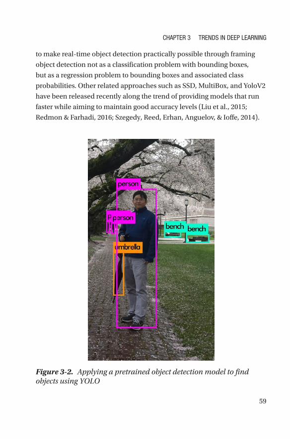
59
to make real-time object detection practically possible through framing
object detection not as a classification problem with bounding boxes,
but as a regression problem to bounding boxes and associated class
probabilities. Other related approaches such as SSD, MultiBox, and YoloV2
have been released recently along the trend of providing models that run
faster while aiming to maintain good accuracy levels (Liu et al., 2015;
Redmon & Farhadi, 2016; Szegedy, Reed, Erhan, Anguelov, & Ioffe, 2014).
Figure 3-2. Applying a pretrained object detection model to find objects using YOLO
ChapTeR 3 TReNds iN deep LeaRNiNg

60
In practice, trade-offs might need to be made between setting up the
solution for accuracy of results versus speed of inference depending on
whether the application has requirements such as real-time performance.
Different meta-architectures, choices made during training such as
the CNN architecture used as the feature extractor, image resolution,
hardware, and software make broad generalizations about the ideal
approach hard to make (J. Huang et al., 2017).
Object SegmentationMany recent proposals explored how to reduce the need for the bounding
box for object detection and explored segmentation neural network
models such as LinkNet, as well as to use more specialized networks for
other vision tasks, such as CortexNet for identifying actions on images
rather than categorizing single frames (Culurciello, 2017). Mask R-CNN
and focal loss for dense object detection are other recent trends in object
detection that have been open sourced by Facebook AI Research within
a software system called Detectron and are thus available to run on the
Microsoft AI Platform (He, Gkioxari, Dollar, & Girshick, 2017; Lin, Goyal,
Girshick, He, & Dollar, 2017). This marks truly exciting progress in object
segmentation!
More Sophisticated Networks The types of networks discussed in this chapter are just some examples
within the broad space of deep learning. There are many ways to formulate
deep neural networks as well as combine with other methodologies within
a broader solution. As an example within the field of speech translation,
Microsoft Research recently found state-of-the-art results on a large
benchmark data set, the English–French translation campaign from 2014
at http://bit.ly/2EzMeRY using what was coined a deliberation network
(Tian, 2017). This network builds on top of a simple LSTM architecture,
ChapTeR 3 TReNds iN deep LeaRNiNg
61
combined with dual learning that is inspired by how humans deliberate.
The premise is simple: A first-pass decoder goes over the sentence similar
to creating a rough draft, whereas the second-pass decoder takes both the
original input as well as the rough draft as input to get to the final solution.
This is just one example, and there are numerous others of combining
deep learning technologies together or with other methodologies as part of
a larger solution as well.
Similar to CNNs and RNNs, there has been large growth in the variety
of proposed types and uses of GANs. There have also already been
many commercial applications of GANs. For example, Microsoft worked
with Getty Images, which provides stock photos, to explore image-to-
image translation, such as turning a sunny beach photo into an overcast
beach photo to provide more options to their customers (Liakhovich,
Barraza, & Lanzetta, 2017). Microsoft Research also developed a “drawing
bot” based on GANs that is able to create images based on only a text
description, images that are based only on the computer’s “imagination”
(Roach, 2018). The AttnGAN model proposed for this purpose was able
to outperform previous state-of-the-art models in early 2018, producing a
nearly threefold boost in image quality for text-to-image generation on an
industry standard test (Xu et al., 2017).
Automated Machine Learning Another area of ML that has been garnering interest the last few years
is that of automatic ML and smart hyperparameter tuning (Bergstra,
Yamins, & Cox, 2013; Domhan, Springenberg, & Hutter, 2015; Fusi &
Elibol, 2017; Golovin et al., 2017; Li, Jamieson, DeSalvo, Rostamizadeh, &
Talwalkar, 2016). Both these areas of research try to make use of historical
information, optimization, and metalearning to be able to automatically
or semiautomatically arrive at optimal ML pipelines, neural network
topologies, and so on.
ChapTeR 3 TReNds iN deep LeaRNiNg
62
Another such piece of work centered around using reinforcement
learning and LSTMs to create new neural network architectures (Zoph &
Le, 2016). Reinforcement learning (RL) is a subfield of AI that is designed
to have software agents automatically determine the optimal behavior to
maximize performance, through a reward feedback process. It is a type of
automated learning mechanism. The resulting CNN architecture called
NASNet achieved state-of-the-art results on the CIFAR10 data set at the
end of 2017 and is 1.05 times faster than the previous state-of-the-art
model. Others have recently focused on more efficient search mechanisms
such as leveraging current networks and reusing trained network weights
(Cai, Chen, Zhang, Yu, & Wang, 2017). In the future we will probably see
further endeavors in this area as computation becomes even quicker and
the scale up and out of cloud infrastructure is fully realized.
Related to architecture search, the field of neuroevolution has recently
received more visibility in the research and industrial community. This is a
subfield of AI that aims to understand and invoke an evolutionary process
similar to the one that produced the form of intelligence in human brains
within a computer. Whereas NASNet and related areas of research focus
on trying to automate the creation of networks, most applications of deep
learning today require a human to specify the architecture of the neural
network. Rather than having a fixed network architecture that we aim to
optimize, researchers in the field of neuroevolution study the process of
learning itself.
Neuroevolution researchers have found interesting results that we
believe will influence more strongly applications of AI in the future. One
example from neuroevolution is the concept of novelty search, the idea
that optimizing for novelty might provide better results than optimizing
for the direct outcome. Stanley (2017) illustrated the concept through the
problem of trying to find a model for a robot to learn how to walk. One
might guess that the best way to get an amazing walking robot would be
to artificially combine together the models of the best walkers from the
previous generation. However, the robots who are good at walking in the
ChapTeR 3 TReNds iN deep LeaRNiNg

63
first generations might just be lurching forward unreliably. In contrast,
robots that try oscillating their legs in a regular pattern fall down right away
but could lead to more robust walking in the future, so simply breeding
based on the best in the past might not be beneficial for the future. This
field has also benefited tremendously by the increased computation power
available today and we expect to see more advances and direct impact on
the deep learning field.
Recently algorithms and processes for deriving AI from the field of
neuroevolution have been applied to the deep learning architecture
search problem and compared against reinforcement learning type
approaches that resulted in NASNet. Real, Aggarwal, Huang, and Le
(2018) found that regularized evolution approaches performed better than
reinforcement learning at early search stages and generally found that
they produced similar or higher accuracy results without having to retune
parameters. The new architecture from this evolutionary search process
called AmoebaNets resulted in state-of-the-art results for several image
classification tasks at the beginning of 2018.
Hardware Deep neural networks involve a vast amount of computation, often
using very large data sets to calculate the composition of an extremely
parameter-heavy model. GPUs, which were originally designed for
computations around rendering graphics on the computer, have
accelerated the use of deep learning because they enable a high
degree of parallelism within the GPU card. GPUs can provide higher
throughput and efficiency for certain categories of applications
compared with CPUs, including the types of computations required
for deep learning training and inference. GPUs have a well-defined
instruction set and fixed data width (specific precision integer and
floating-point values).
ChapTeR 3 TReNds iN deep LeaRNiNg

64
GPUs have become increasingly more powerful over time, as
mentioned in Chapter 2. For example, the release of the NVIDIA Tesla
V100 in May 2017 touted 2.4 times faster training of ResNet-50 DNN than
the P100 released a year earlier (Durant, Giroux, Harris, & Stam, 2017).
In addition, there has been recent research on mixed precision training,
allowing for a reduction in the memory consumption and thus shortening
the training or inference time (Micikevicius, 2017).
More Specialized HardwareHardware has continued to specialize with the specialization of field
programmable gate arrays (FPGAs) and application-specific integrated
circuits (ASICs) for neural network modeling, moving toward more
specialized hardware that is more efficient, as pictured in Figure 3-3.
FPGAs are integrated circuits that do not have a predefined instruction
set or fixed data width like GPUs. FPGA acceleration works by having
the FPGA handle the extremely computing-intensive tasks that have
been designed to be accelerated by the hardware, while the CPU handles
other operations. They provide potential for ultralow latency calculations
through optimizing numerical precision for inference, as well as potential
to evolve to new ML application areas. They can run low-precision
workloads for optimal efficiency using much less power and thus run
much cheaper than GPUs.
Increasing use of FPGA technology is an especially promising trend in
the AI space because of FPGA’s reconfigurability and its access to both the
hardware and software level. This is especially promising for its potential
for compromise between flexibility and specialization. ASICs are more
performant for the application for which they are designed, but they are
not useful for general-purpose computing, as they cannot be reconfigured
after manufacturing.
ChapTeR 3 TReNds iN deep LeaRNiNg

65
In other words, FPGAs are more flexible than ASICs as they can be
used and then repurposed for workloads beyond just deep learning and
AI applications, including graph analytics, database acceleration, and
data encryption, for example. Programming FPGAs requires support from
specialized compilers, and it is relatively much harder than compilers used
for traditionasl processors.
Hardware on AzureMicrosoft has been investing in specialized hardware for use both in
their own products as well as for others to use through their Azure cloud
computing platform. To accelerate Bing’s search ranking algorithm, for
example, FPGAs were programmed for that sole purpose and resulted in
double the throughput at just 10 percent more power (Feldman, 2016).
In 2016, Altera FPGAs were installed across every Azure cloud server
datacenter at the time as Microsoft prepared to release capabilities as
third-party offering. The ability to use FPGAs for deep learning inference that
was announced in early 2018 is mentioned in more detail in Chapter 10.
Quantum Computing As hardware such as more advanced GPUs and FPGAs continues to advance
and specialize to enable deep learning, the future of how computing is
conducted might also change dramatically in the longer term thanks
Figure 3-3. Alternatives for processing computations such as those in deep learning models
ChapTeR 3 TReNds iN deep LeaRNiNg
66
to ongoing research in areas such as quantum computing. Quantum
computing is a fundamentally different way of computing compared to
today’s computers. Rather than the foundational building block of a bit in
today’s computers, quantum computing builds on quantum bits called
qubits that exist as a mixture of states at a given point in time and that can
be manipulated all at once. It’s not clear yet what types of problems are
most applicable to quantum computing, although there are some clear
applications such as cryptography. Unfortunately, building quantum
computers is extremely difficult and they are extremely hard to use as well as
scale. So far, they can only be used for a limited set of computing tasks. Qubits
are extremely sensitive to the surrounding environment and interference
results in calculation errors. Microsoft is working on developing more general-
purpose quantum computers to help solve today’s intractable problems
through research on “topological qubits” that has the potential to completely
revolutionize AI by opening up completely new computing potential.
The problems we’re looking at solving with a quantum com-puter are the problems that, today, require age-of-the-universe time scales. … Some of these problems literally require billions and billions and billions of years to solve. And on a quantum computer, what we’ve shown in some recent research, is that you can solve some of these problems in a matter of say, weeks, days, hours, seconds.
—Krysta Svore, Microsoft Research
Although this is an area of active research, Microsoft has released
quantum computing development tools and programming language
for quantum algorithm development. Other areas of research include
approximate computing, using less precision as well as allowing random
small mistakes that can cancel out over time, to save energy and increase
efficiency of computations. Many believe quantum computing has much
potential to accelerate the development and application of AI, but the full
power and potential is yet to be seen.
ChapTeR 3 TReNds iN deep LeaRNiNg

67
Limitations of Deep LearningDeep learning has led to many incredible advances in the application of AI.
Deep neural networks work by transforming an input vector to a target
output vector, a complicated transformation created simply through a
series of simple transformations. With massive data and computing power,
the relatively simple concept of neural network models can be used to
effectively map between many inputs and outputs such as recognizing
speech from audio snippets. We believe deep learning will continue to
play a large role in the advancement of AI applications, but that we need to
understand the limits and capabilities to apply the technology in the right
scenarios and in appropriate ways.
Be Wary of HypeIn fact, we should be careful not to overestimate the abilities of deep
learning models. They do not learn abstract concepts or “understand” in
a way that is relatable to humans. From an early age, humans are able to
reason and maintain abstract models of the world, consider hypothetical
situations, and make decisions through critical thinking. These neural
networks importantly cannot reason or do long-term planning in this way
and by themselves do not represent any type of general intelligence. After
all, even if an algorithm can predict what an object is, that does not imply
the algorithm actually understands the properties of the object, how it
would interact with its environment, what it is used for, or where it came
from. So, although computers can learn from massive data to distinguish
between different types of birds better than humans, for example, humans
are still far superior at extrapolation, interpretation, and inference, such as
understanding a complex scene.
Similarly, in natural language processing, humans are able to understand
nuances in aspects such as word ordering and context, whereas neural
network models struggle to understand broader abstract concepts and
ChapTeR 3 TReNds iN deep LeaRNiNg
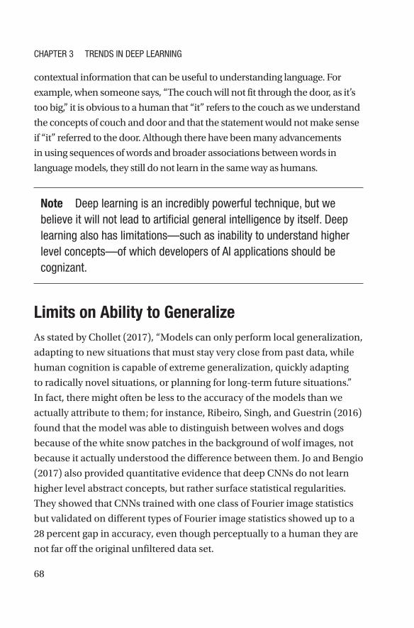
68
contextual information that can be useful to understanding language. For
example, when someone says, “The couch will not fit through the door, as it’s
too big,” it is obvious to a human that “it” refers to the couch as we understand
the concepts of couch and door and that the statement would not make sense
if “it” referred to the door. Although there have been many advancements
in using sequences of words and broader associations between words in
language models, they still do not learn in the same way as humans.
Note deep learning is an incredibly powerful technique, but we believe it will not lead to artificial general intelligence by itself. deep learning also has limitations—such as inability to understand higher level concepts—of which developers of ai applications should be cognizant.
Limits on Ability to GeneralizeAs stated by Chollet (2017), “Models can only perform local generalization,
adapting to new situations that must stay very close from past data, while
human cognition is capable of extreme generalization, quickly adapting
to radically novel situations, or planning for long-term future situations.”
In fact, there might often be less to the accuracy of the models than we
actually attribute to them; for instance, Ribeiro, Singh, and Guestrin (2016)
found that the model was able to distinguish between wolves and dogs
because of the white snow patches in the background of wolf images, not
because it actually understood the difference between them. Jo and Bengio
(2017) also provided quantitative evidence that deep CNNs do not learn
higher level abstract concepts, but rather surface statistical regularities.
They showed that CNNs trained with one class of Fourier image statistics
but validated on different types of Fourier image statistics showed up to a
28 percent gap in accuracy, even though perceptually to a human they are
not far off the original unfiltered data set.
ChapTeR 3 TReNds iN deep LeaRNiNg
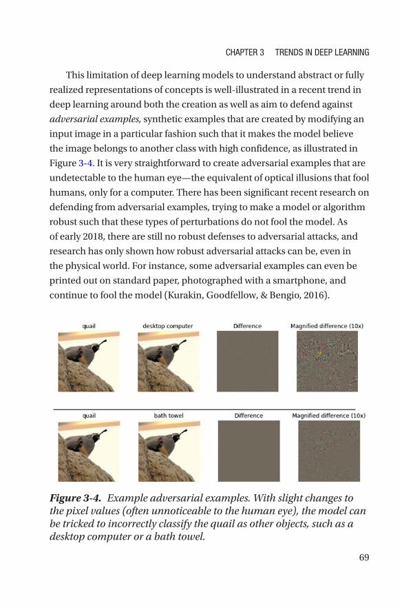
69
This limitation of deep learning models to understand abstract or fully
realized representations of concepts is well-illustrated in a recent trend in
deep learning around both the creation as well as aim to defend against
adversarial examples, synthetic examples that are created by modifying an
input image in a particular fashion such that it makes the model believe
the image belongs to another class with high confidence, as illustrated in
Figure 3-4. It is very straightforward to create adversarial examples that are
undetectable to the human eye—the equivalent of optical illusions that fool
humans, only for a computer. There has been significant recent research on
defending from adversarial examples, trying to make a model or algorithm
robust such that these types of perturbations do not fool the model. As
of early 2018, there are still no robust defenses to adversarial attacks, and
research has only shown how robust adversarial attacks can be, even in
the physical world. For instance, some adversarial examples can even be
printed out on standard paper, photographed with a smartphone, and
continue to fool the model (Kurakin, Goodfellow, & Bengio, 2016).
Figure 3-4. Example adversarial examples. With slight changes to the pixel values (often unnoticeable to the human eye), the model can be tricked to incorrectly classify the quail as other objects, such as a desktop computer or a bath towel.
ChapTeR 3 TReNds iN deep LeaRNiNg
70
Data Hungry Models, Especially LabelsDeep learning models also are limited by the vast amount of data that
is required to train the network. This is especially made difficult by the
requirement for high-quality, curated labels from which the model
can learn. Although techniques such as transfer learning and word
embeddings as mentioned earlier are able to somewhat alleviate this
problem in some contexts, deep learning is not able to learn from explicit
definitions or complete many types of tasks that are not simple input
to output pairings. Although incredibly powerful, it is clear that deep
learning alone is not a solution for artificial general intelligence. As
another example, deep learning even struggles to represent a basic sorting
algorithm.
Many of these limitations of deep learning are actually limitations of
ML algorithms in general, such as the inability to inherently distinguish
correlation from causation. After all, deep learning is simply a statistical
technique that excels at optimizing a mapping from an input to an output.
However, unlike some simpler methodologies, explaining the solutions of
deep neural networks can be extremely difficult. Engineering the network
as needed can also be quite hard, such as trying to debug when something
goes wrong or when one wants to tune a specific aspect of the modeling
results. Although deep learning has many limits and is just one tool that
can be used among many, we believe that deep learning will serve as a
stepping stone to many future advances in AI, as we discuss later.
Reproducible Research and Underlying Theory With the rise in popularity of deep learning, the number of research
papers has increased dramatically every year. Recently, researchers
have begun raising more concerns about the reproducibility of these
papers, for example, when code is not released or specific details
that are important to reproduce the result are not included. This is
ChapTeR 3 TReNds iN deep LeaRNiNg

71
exacerbated by the lack of theoretical understanding about how to best
develop these type of networks as well as optimize them, in addition to
how many of the papers in the field require vast computing resources to
reproduce. In practice, overfitting is common and very different results
can be obtained depending on the type of evaluation method and split
of the data.
Rahimi recently brought this issue of lack of theoretical underpinning
to light in his December 2017 NIPS talk “Machine Learning Has Become
Alchemy.” His point was that we lack clear theoretical explanations
of why deep learning works and how to understand when it does not,
often called the black box problem. An example exception is the idea
of information bottleneck, which posits a network gets rid of the noisy
extraneous details like squeezing the information through a bottleneck,
and only the features that are relevant to general concepts are retained
(Tishby & Zaslavsky, 2015). Others have also cautioned that theory in
general often lags behind empirical results and that being too cautious
has the risk of leading to another “AI Winter,”1 when instead continued
research into how models can be used to solve real problems can propel
us forward.
Nonetheless, it is clear that deep learning works for many
applications in practice and is a useful tool for practitioners, and we
need to understand both its usefulness and its weaknesses so that AI
can continue bringing more value to society in the future. We believe
the more open the community can be, in terms of publishing code
associated with research as well as data when possible, the more it will
help the field progress forward.
1 Lighthill released a report in 1973 that suggested AI was a failure and too superficial to be used in practice, leading to a massive reduced interest in the field.
ChapTeR 3 TReNds iN deep LeaRNiNg

72
Looking Ahead: What Can We Expect from Deep Learning?Although acknowledging deep neural networks are a statistical
methodology with many limits, we are optimistic that deep neural
networks will be used as a foundational building block within an
increasing number of more sophisticated methodologies that will emerge
over time. The use of dynamic networks, for example, which uses deep
neural networks but allows the networks to change dynamically as a
function of the data fed into the model over time, has risen recently.2 The
combination of deep neural networks embedded within reinforcement
learning systems has also solved increasingly complex problems. LeCun
(2018) suggested that “differentiable programming” should be the
rebranding of deep learning to mark the transformation toward a new
type of software that is differentiable and optimizable. Karpathy (2017)
suggested that “[n]eural networks are not just another classifier, they
represent the beginning of a fundamental shift in how we write software …
they are Software 2.0.”.
We expect research will continue to propel the practicality of deep
learning forward, such as potential breakthroughs in optimizing neural
network architectures as discussed earlier. Some areas of research are
also still largely unsolved, such as the ability to learn from unlabeled
data, also known as unsupervised learning, where there is much room
for innovation. Additionally, we expect more work to focus on program
synthesis and graph networks, as well as more applications of adversarial
networks.
2 Frameworks such as MXNet/Gluon, PyTorch, and Chainer support these types of networks, and we expect this trend to continue.
ChapTeR 3 TReNds iN deep LeaRNiNg
73
Ethics and Regulations Finally, it is clear that there are ethical concerns, around aspects such
as bias, security, privacy, and appropriate use of deep learning and AI
technologies. These ethical considerations will start to increasingly affect
the development of AI systems as laws and regulations are enacted to
constrain the impact of these systems. As mentioned earlier, for example,
deep learning systems today are vulnerable to adversarial examples,
even in the physical world, which poses a security risk. Then besides the
security implications, there are ethical considerations around bias as well.
Bias in AI and ML algorithms is typically described and studied
in terms of statistical bias, a mathematical construct to describe the
difference between an expected value and the true value of the parameter
being estimated. Depending on the type of model, bias can be introduced
in different ways. But even when a system is not mathematically biased, it
can be biased in the popular culture’s interpretation of the word.
The popular culture definition of bias is normally associated with some
form of prejudice or preferential treatment toward a particular group. This is
usually felt to be unfair. It should be noted that fairness is culturally defined
and varies throughout history. Therefore, unfairness is really in the application
of bias. The tricky part about this is that people normally assume that
computers will be unbiased, and that the outcomes made from mathematical
models will be fairer than those made by humans. By their very nature,
though, deep learning models will display some bias in this sense of the
word, because the driving force in them is the real-world data on which these
models are built. Unfortunately, these true historical data are rooted with bias.
For some applications of deep learning where there are high-stakes
outcomes such as hiring or loan applications, it is clear that this can have
very detrimental effects. Take, for example, the use of word embeddings
that represent words in a lower dimensional space. It is clear that word
embeddings are biased, an example being word embeddings trained on
Google News articles. These word embeddings have biased embedded
ChapTeR 3 TReNds iN deep LeaRNiNg

74
relationships between words that can be extracted very easily such as
“man is to computer programmer as women is to homemaker” (Bolukbasi,
Chang, Zou, Saligrama, & Kalai, 2016). This can have detrimental effects on
applications of deep learning with word embeddings when applied without
consideration of these type of issues. For example, recruiters are increasingly
using algorithms to automatically match resumes to job openings. If word
embeddings are applied blindly within this process, however, and historical
data favors that “successful” people in the role were mostly men, the
outcomes of this process can be argued to be detrimental. O’Neil (2016),
in her book Weapons of Math Destruction, outlined many ways in which
algorithms can be used to a detrimental effect in the era of big data, and it is
important to be cognizant of the potential for harm.
Unfortunately, bias can be difficult to detect and remove. In 2015 as
another example, a photo application improperly labeled a dark-skinned
person as a “gorilla,” which prompted a quick and immediate apology. Had
the company been aware of this, they surely would not have deployed this
technology. AI and ML predictive modeling is inherently more difficult to
test than traditional software applications, however. After all, in a classical
software system, an input will generate a known output, but this is not
true for AI-based systems. AI-based systems are evaluated based on their
statistical results and these results can often change from one run of the
data to the next. Unless adequate testing methodologies for AI-based
systems are developed, deploying AI-based systems could encounter
major roadblocks to deployment.
Not only are there ethical and cultural issues, but there are a host of
legal implications as well. Fortunately, bias in ML applications has become
increasingly discussed in both the research and industry communities.
However, it is important to recognize that technological advances alone
will not solve the problem; there is no one-size-fits-all solution to this.
Testing of AI models and development of fair systems will undoubtedly
require an interdisciplinary approach to achieve the goal of building safe,
widely distributed AI.
ChapTeR 3 TReNds iN deep LeaRNiNg

75
SummaryThis chapter discussed some of the trends in the deep learning space,
such as the search for optimal network architectures both for accuracy as
well as speed. We also went through two recent exciting developments in
neural networks for computer vision, the first tackling the limitations of
CNNs through capsule networks and the other using neural networks to try
and define optimal architectures with minimal human intervention with
automated ML techniques.
We discussed several other trends in deep learning, including more
specialized hardware as well as the use of pretrained models to seed
solutions with fewer data than required to build a deep learning solution
from scratch. We finally discussed some limitations of deep learning
of which developers should be cognizant, such as the inability of these
models to understand abstract concepts, as well as some of the legal and
ethical concerns, including adversarial examples and bias in models from
the underlying data on which they are built.
Next Chapter 4 describes how you can use the tools, infrastructure,
and services on the Microsoft AI Platform to manage the development life
cycle of your deep learning projects and models, to train at scale, and to
operationalize it quickly as web APIs.
ChapTeR 3 TReNds iN deep LeaRNiNg
PART II
Azure AI Platform and Experimentation Tools

79© Mathew Salvaris, Danielle Dean, Wee Hyong Tok 2018 M. Salvaris et al., Deep Learning with Azure, https://doi.org/10.1007/978-1-4842-3679-6_4
CHAPTER 4
Microsoft AI PlatformThis chapter introduces the Microsoft AI Platform, which is a set of
services, infrastructure, and tools for building intelligent applications
powered by AI. The Microsoft AI Platform runs on the Microsoft Azure
cloud computing environment, which provides computing as a utility
where you pay for what you use rather than what you own. For more
details on the broader Azure Platform, please see the e-book Developer’s
Guide to Microsoft Azure (Crump & Luijbregts, 2017). The Microsoft AI
Platform enables data scientists and developers to create AI solutions in an
efficient and cost-effective manner.
Although Microsoft has other offerings for developing AI solutions
such as Machine Learning Server, which can be deployed on-premises
in addition to the cloud as well as hybrid offerings, this chapter focuses
primarily on the cloud computing platform that for reasons described later
is most applicable to developing deep learning solutions. In practice, the
models developed with the Microsoft AI Platform can then be deployed
in many locations such as on the cloud for real-time highly scalable
applications, on the edge through Azure IOT, or within a database such as
a stored procedure hosted within SQL Server, for example. The Microsoft
AI Platform is a flexible, open, enterprise-grade set of services, tools, and
infrastructure that allow developers and data scientists to maximize their
productivity in developing AI solutions.
80
Developing a deep learning solution requires lots of experimentation,
lots of computing power—often using advanced hardware such as GPUs and
FPGAs as discussed in Chapter 3, and often lots of training data. There is a
need to be able to run training at scale. Cloud computing, with the ability
to scale up and down easily with various levels of management—from raw
infrastructure to managed services—makes doing data science including
training and scoring deep learning models a more practical reality.
In fact, developing a deep learning solution requires carefully setting
up many aspects, such as data storage, development environment,
scheduling for training and scoring, cluster management, and managing
costs, among other aspects. Deep learning solutions are notorious for
their difficult configurations, such as ensuring drivers and software
compatibility. It is important to store data in a location that can scale with
increasing volume and enable collecting more data to improve solutions
over time. These data must also be stored in a location that is secure and
compliant with local regulations. Development environments must fit
the needs of the developer or data scientist creating the code and allow
workflows such as moving from a laptop to the cloud. Deep learning
training workflows must be scheduled and monitored. The Azure cloud
computing environment enables scaling up and down for cost control,
has various levels of product offerings to address these aspects, from
raw infrastructure with VMs already configured for deep learning to fully
managed services with pretrained models ready to consume.
Of course, not all these services are necessary for a single given
solution, but rather taken together provide a platform on which any type
of intelligent application can be built leveraging the best of open-source
technology as well as decades of research within Microsoft on both AI
algorithms as well as tooling for development. By building on top of the
Azure platform, developers and data scientists can leverage infrastructure
that scales virtually infinitely, with enterprise-grade security, availability,
compliance, and manageability. In the sections that follow, the main
Chapter 4 MiCrosoft ai platforM
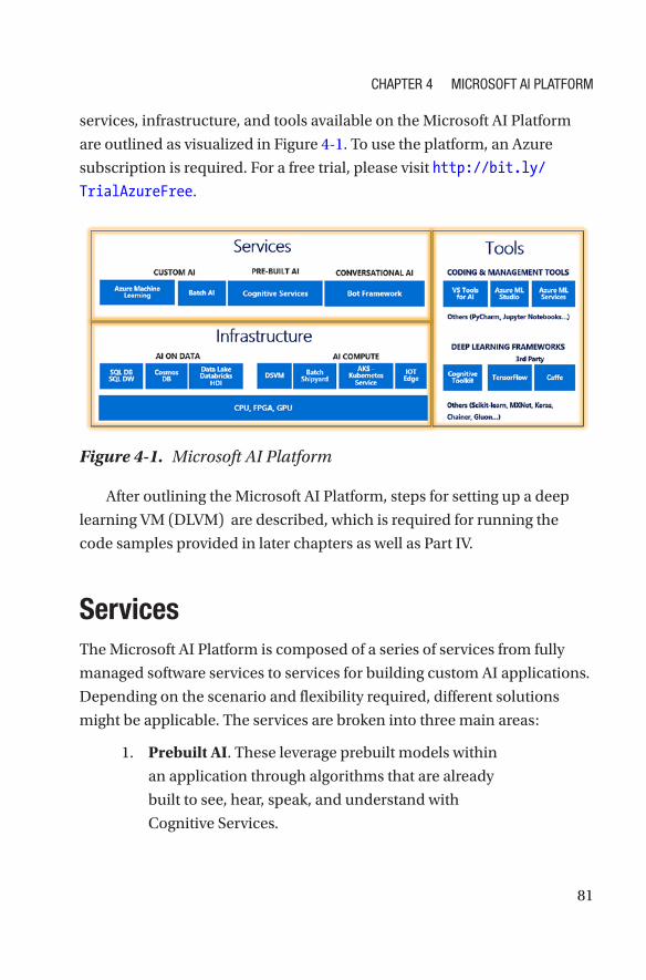
81
services, infrastructure, and tools available on the Microsoft AI Platform
are outlined as visualized in Figure 4-1. To use the platform, an Azure
subscription is required. For a free trial, please visit http://bit.ly/
TrialAzureFree.
Figure 4-1. Microsoft AI Platform
After outlining the Microsoft AI Platform, steps for setting up a deep
learning VM (DLVM) are described, which is required for running the
code samples provided in later chapters as well as Part IV.
ServicesThe Microsoft AI Platform is composed of a series of services from fully
managed software services to services for building custom AI applications.
Depending on the scenario and flexibility required, different solutions
might be applicable. The services are broken into three main areas:
1. Prebuilt AI. These leverage prebuilt models within
an application through algorithms that are already
built to see, hear, speak, and understand with
Cognitive Services.
Chapter 4 MiCrosoft ai platforM

82
2. Conversational AI. These build natural interaction
into an application through the Bot Framework,
which has connectors to common channels such as
Facebook Messenger, Slack, Skype, and Bing.
3. Custom AI Services. These adapt to a scenario with
the flexibility of Azure Machine Learning services,
Batch AI service or both.
Prebuilt AI: Cognitive ServicesCognitive Services are a set of services available to developers and data
scientists to build AI solutions, with capabilities around vision, speech,
language, knowledge, and search (see Table 4-1). The Cognitive Services
are of two main types:
1. Pretrained models available as REST APIs, ready
to consume in end user applications without any
customization required.
2. Bring-your-own-data services, such as Custom
Vision Service, which allows a developer to create
a custom image classification model without any
background in computer vision or deep learning by
simply uploading images of different classes and
clicking a button to train the model.
Chapter 4 MiCrosoft ai platforM
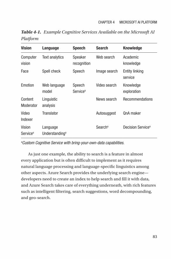
83
As just one example, the ability to search is a feature in almost
every application but is often difficult to implement as it requires
natural language processing and language-specific linguistics among
other aspects. Azure Search provides the underlying search engine—
developers need to create an index to help search and fill it with data,
and Azure Search takes care of everything underneath, with rich features
such as intelligent filtering, search suggestions, word decompounding,
and geo- search.
Table 4-1. Example Cognitive Services Available on the Microsoft AI
Platform
Vision Language Speech Search Knowledge
Computer
vision
text analytics speaker
recognition
Web search academic
knowledge
face spell check speech image search entity linking
service
emotion Web language
model
speech
servicea
Video search Knowledge
exploration
Content
Moderator
linguistic
analysis
News search recommendations
Video
indexer
translator autosuggest Qna maker
Vision
servicea
language
Understandinga
searcha Decision servicea
aCustom Cognitive Service with bring-your-own-data capabilities.
Chapter 4 MiCrosoft ai platforM
84
These services are popular, as they are simple to add into applications.
Just a few lines of code are required to integrate a model such as an emotion
detection model into a customer service experience application. Given the
breadth of Cognitive Services and Custom Cognitive Services available for
use today, these services are described in more depth in the Chapter 5.
Conversational AI: Bot FrameworkThe Bot Framework includes tools and services to enable developers to
build bots that converse with users. For example, a developer can easily
develop a bot that interacts with users on a web site to guide them through
purchasing a product or service rather than having to navigate through
the web page. Through this framework, one can develop once and then
expose the bot through many channels that are included within the Bot
Framework, such as Skype, Facebook, and the Web. Bots can be built with
the Bot Builder Software Development Kit (SDK) using C# or Node.js or
with the Azure Bot Service.
Bots can be built to converse naturally, especially using advanced
capabilities with integration of Cognitive Services such as the Language
Understanding Intelligence Service (LUIS) and integrations with other
cognitive services. As a managed service in Azure, it is scalable, and costs
are only occurred for the resources that are used.
Custom AI: Azure Machine Learning ServicesAzure Machine Learning services were released in public preview in late
2017. These services are useful for building custom AI solutions and helping
to accelerate the end-to-end development of intelligent applications.
• Develop, deploy, and manage models at scale.
• Develop with the tools and frameworks popular in the
open source community.
Chapter 4 MiCrosoft ai platforM
85
Azure Machine Learning services provide a framework to manage a
data science project. With these services, one can bring the computing
environment most applicable for training their AI models, for example:
1. Data Science Virtual Machine.
2. Spark on Databricks or HDInsight.
3. Azure Batch AI.
These computing environments are described later in this chapter.
The experimentation service helps to manage project dependencies,
scale out training jobs, and enable sharing of data science projects. Model
management service uses docker container-based deployment to help
data scientists and developers deploy solutions on a single node (on the
cloud or on-premises) as well as scale out cluster deployments such as
Azure Container Services, as well as edge deployment via Azure IOT Edge.
As of this writing, Azure Machine Learning services works with
Python and is available in several Azure regions. In addition, there are
AI extensions for Visual Studio and Visual Studio Code discussed in the
“Tools” section later in this chapter that allow interacting with the Azure
Machine Learning platform (http://bit.ly/aivisstdio). As the service
is updating frequently, we focused on the core computing environments
in this book and suggest reading the current documentation on Azure
Machine Learning services available at http://bit.ly/AMLservices.
Custom AI: Batch AIBatch AI is a managed service that enables data scientists and developers
to easily train deep learning and other AI models at scale with clusters
of GPUs. With Batch AI, one can create a clusters of nodes including
GPUs when required, and then turn the cluster off when the job is
complete and thus stop the bill. It allows one to construct a framework-
specific configuration using either containers or VMs. This is ideal for
Chapter 4 MiCrosoft ai platforM
86
experimentation, such as doing parameter sweeps or experiments,
testing different network architectures, or doing hyperparameter tuning
in general. It also enables multi-GPU training for frameworks that allow
training across nodes when training data are very large. An example
with associated code for training deep learning models with Batch AI
is included in Chapter 9. Batch AI can also be used for embarrassingly
parallel batch scoring scenarios.
Batch AI is built on top of Azure Batch, which is a cloud-scale
resource management and task execution tool. With Batch AI, you only
pay for the computing that you use, with both standard and low-priority
VMs available. There is no added charge for job scheduling or cluster
management in general. Low-priority VMs provide a cost-efficient solution
for jobs that are lower priority, such as learning and experimentation.
Related to Batch AI, Batch Shipyard is an open source tool that is a
precursor to the managed Batch AI service that also runs on top of the
Azure Batch infrastructure. Batch Shipyard supports both Docker and
Singularity containers and scenarios important to developing deep
learning solutions such as hyperparameter tuning. Batch Shipyard can also
be utilized for batch scoring of deep learning models. More details about
Batch AI and Batch Shipyard can be found in Part IV of the book.
InfrastructureIn this section, we outline infrastructure available for AI computing,
such as the Data Science Virtual Machine (DSVM), Spark clusters,
and infrastructure for managing deployment of containers as well as
infrastructure for storing data on which AI can be built such as SQL DB,
SQL Datawarehouse, Cosmos DB, and Data Lake.
Chapter 4 MiCrosoft ai platforM
87
Data Science Virtual MachineThe DSVM is a preconfigured environment in the cloud for data science
and AI modeling, development, and deployment. It comes in a Windows
Server version as well as Linux, and a specialized version for deep learning
known as DLVM, which runs on a GPU. As can be seen in Figure 4-2,
popular languages for data science development such as Python, R, and
Julia are ready to use immediately, and data connected from many data
stores such as SQL Data Warehouse, Azure Data Lake, Azure Storage, and
Azure Cosmos DB are available. Many ML and AI tools come preinstalled,
such as many of the popular deep learning frameworks. Data scientists
and developers can then customize the VM as needed for their use. There
is also a variant specialized for geospatial analysis, the Geo AI DSVM:
http://aka.ms/dsvm/geoai/docs.
DSVMs are extremely popular with data scientists for the following
reasons:
• They provide an analytics desktop in the cloud with
easy setup, and the ability to transfer projects more
easily between colleagues.
• They have on-demand elastic capacity, ability to turn
off and on (e.g., stopping the VM at night if no jobs are
running).
• There are examples and templates built in to get started
with data science and deep learning.
• There is an ability to connect into other services such as
using DSVM as the computing target within a project
managed through Azure Machine Learning services or
as compute for Batch AI service.
• They are easy to use for data science training and
education due to ease of setup and cost savings versus
purchasing hardware and managing the software oneself.
Chapter 4 MiCrosoft ai platforM
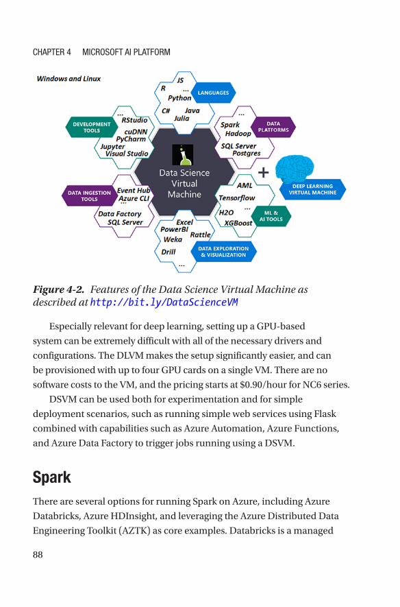
88
Especially relevant for deep learning, setting up a GPU-based
system can be extremely difficult with all of the necessary drivers and
configurations. The DLVM makes the setup significantly easier, and can
be provisioned with up to four GPU cards on a single VM. There are no
software costs to the VM, and the pricing starts at $0.90/hour for NC6 series.
DSVM can be used both for experimentation and for simple
deployment scenarios, such as running simple web services using Flask
combined with capabilities such as Azure Automation, Azure Functions,
and Azure Data Factory to trigger jobs running using a DSVM.
SparkThere are several options for running Spark on Azure, including Azure
Databricks, Azure HDInsight, and leveraging the Azure Distributed Data
Engineering Toolkit (AZTK) as core examples. Databricks is a managed
Figure 4-2. Features of the Data Science Virtual Machine as described at http://bit.ly/DataScienceVM
Chapter 4 MiCrosoft ai platforM
89
platform for Spark with a rich experience for both data scientists and
developers, such as a team collaboration experience and version control
capabilities. The service handles much of the tuning of the cluster for
developers, so is thus ideal for users who might not know or want to
configure Spark, but it is not as flexible in terms of how the cluster can be
configured. HDInsight is a fully managed cloud service for open source
analytics such as HBase, Hive, Storm, and others in addition to Spark.
The AZTK is an open source Python Command-Line Interface (CLI)
application for provisioning on-demand Spark clusters in Azure. The Spark
clusters run in Docker containers with bring-your-own Docker image
flexibility and are provisioned within 5 minutes on average, with low-priority
VMs available for an 80 percent discount. This toolkit is useful for running
a distributed Spark workload on demand such as batch workloads and
can be scheduled to spin up and down such as through the use of Azure
Functions. It has a rich Python SDK for programmatic control of clusters and
jobs. AZTK is the most flexible option in terms of supporting all VM types
including GPUs, which is especially helpful for deep learning scenarios.
For all of these Spark infrastructure options, Microsoft Machine
Learning for Apache Spark (MMLSpark) provides a number of deep
learning and data science tools for Apache Spark including integration
with the deep learning framework CVTK. Spark has also seen recent
improvements in support for deep learning applications through
collaborations aimed toward improving support for aspects such as image
data support as discussed at http://bit.ly/SparkImage.
Container HostingAzure Kubernetes Service (AKS) is a fully managed Kubernetes container
orchestration service. Users might also choose other orchestrators through
the original version, known as ACS. With the fully managed version of
AKS, the only cost is for the VMs that are used for the tasks at hand; in
other words, the management infrastructure is completely free. AKS is
Chapter 4 MiCrosoft ai platforM
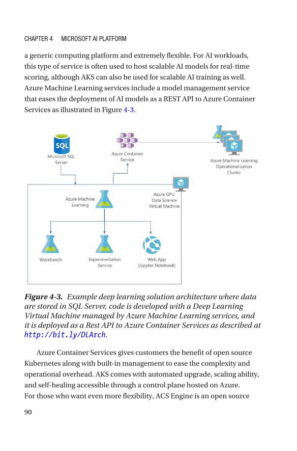
90
a generic computing platform and extremely flexible. For AI workloads,
this type of service is often used to host scalable AI models for real-time
scoring, although AKS can also be used for scalable AI training as well.
Azure Machine Learning services include a model management service
that eases the deployment of AI models as a REST API to Azure Container
Services as illustrated in Figure 4-3.
Figure 4-3. Example deep learning solution architecture where data are stored in SQL Server, code is developed with a Deep Learning Virtual Machine managed by Azure Machine Learning services, and it is deployed as a Rest API to Azure Container Services as described at http://bit.ly/DLArch.
Azure Container Services gives customers the benefit of open source
Kubernetes along with built-in management to ease the complexity and
operational overhead. AKS comes with automated upgrade, scaling ability,
and self-healing accessible through a control plane hosted on Azure.
For those who want even more flexibility, ACS Engine is an open source
Chapter 4 MiCrosoft ai platforM

91
project that allows developers to build and use custom Docker-enabled
container clusters.
Developers can also host containers using Azure Container Instances,
where a container can be hosted without a container orchestrator, which
is especially useful for testing or hosting a simple application that does
not require scaling. Azure App Service is a collection of hosting and
orchestration services comprised of Web App, Web App for Containers,
and Mobile App. Web App, for example, enables developers to host web
applications or APIs whereas Web App for Containers enables one to
deploy and run containerized web apps with images from Docker Hub or a
private Azure Container Registry.
Data StorageAzure SQL Database is a relational cloud database as a service, with built-
in intelligence, specially built for applications with individual updates,
inserts, and deletes (OLTP). Azure SQL Data Warehouse is a warehouse not
strictly for OLTP workloads in that it is desired to be more straightforward
to use for larger databases, with additional feature ability to pause to save
on costs. SQL Database supports more active connections and concurrent
queries than SQL Data Warehouse, whereas SQL Data Warehouse supports
Polybase, which is a technology that accesses data outside of the database
via the T-SQL language. Often these services are used in conjunction with
a larger data architecture.
Azure Cosmos DB is a globally distributed, multimodel database
service that enables extremely low latency and massively scalable
applications. It has native support for NoSQL and can support key-value,
graph, column, and document data all in one service. Several different
APIs including SQL, Apache Cassandra, and MongoDB can be used to
access data, and multiple consistency choices are offered for low-latency
and high-availability options such as strong, bounded staleness, and
eventual. This offering is extremely useful for disparate types of data.
Chapter 4 MiCrosoft ai platforM
92
Azure Data Lake Store is a no-limits data lake that stores unstructured,
semistructured, and structured data, which are optimized for big data
analytics workloads. It is massively scalable and built to the open Hadoop
Distributed File System (HDFS) standard, thus integrating into many tools
easily and allowing a straightforward migration of existing Hadoop and
Spark data to the cloud. Data Lake Store can store trillions of files and a
single file can be larger than one petabyte in size. Azure Blob Storage is
a separate storage option that is a more general-purpose object store,
including for big data analytics workloads, and comparison between them
can be found at http://bit.ly/LakeVBlob.
ToolsSeveral tools and toolkits for developing and deploying AI solutions were
mentioned within the previous sections as they related to services and
infrastructure for AI, such as AZTK for deploying a Spark infrastructure and
Batch Shipyard for executing batch and High Performance Computing (HPC)
container workloads. In this section, we include a nonexhaustive summary of
several other tools that are available on the Microsoft AI Platform.
Azure Machine Learning StudioAzure Machine Learning Studio is a serverless environment for training
and deploying ML models. Studio provides a graphical user interface
(GUI) with the ability to drag and drop easily configured modules for data
preparation, training, scoring, and evaluation. Many prebuilt algorithms
are included for common scenarios such as regression and classification,
and extensibility is enabled through R and Python scripting modules
where custom code can be inserted and connected to other modules.
Although it is extremely useful for quickly developing custom ML solutions
on smaller data set sizes, we do not recommend Azure Machine Learning
Chapter 4 MiCrosoft ai platforM
93
Studio for developing deep learning solutions, as the size of input data is
limited, as well as the hardware it is run on. Today, there is no ability to
bring your own computing environment or manage scale-out computing
across nodes with Azure Machine Learning Studio. Because of these
factors, we recommend Azure Machine Learning services for developing
deep learning solutions instead.
Integrated Development EnvironmentsWith Microsoft Azure, any integrated development environment (IDE) or
editor can be used to create AI applications. In several of the popular IDEs,
there are plug-ins or extensions available that make it even simpler, such
as publishing directly to Azure. For example, Visual Studio Code Tools
for AI is an extension for Visual Studio Code that is a cross-platform open
source IDE. Visual Studio Tools for AI is an extension for Visual Studio
for developing AI applications with an ability to set remote computing
contexts. At the time of this writing, we recommend using Visual Studio
Tools for AI and include an example using this later in this chapter.
These IDEs have nice features to accelerate development, but, of
course, other popular IDEs such as PyCharm and RStudio can be used
to develop the code that will run on the Microsoft AI Platform and
more extensions will become available over time. In addition, Jupyter
notebooks can be leveraged and is already set up for development on the
DSVM. Azure Notebooks are another option for running code with hosted
Jupyter notebooks; Azure Notebooks is completely free, but these do not
run on GPUs so are not as practical for deep learning solutions.
Deep Learning FrameworksThe Microsoft AI Platform is an open platform that builds on the best
of open source technology. Deep learning frameworks such as the
Microsoft Cognitive Toolkit (CNTK), Tensorflow, Caffe, and PyTorch,
Chapter 4 MiCrosoft ai platforM
94
which are all open source projects, are supported throughout many of
the tools, services, and infrastructure already mentioned. The DLVM
comes preconfigured with many of the popular frameworks, and these
frameworks can be used to develop AI solutions and be deployed on
Azure, on Azure IOT Edge, or Windows Machine Learning, for example.
These frameworks were discussed in more detail in Chapter 2.
Broader Azure PlatformIn practice, there are many other components of Azure that are often used
to build AI solutions, to complement the AI-specific services with other
requirements such as dealing with ingestion and processing of streaming
data flows, authentication, and dashboarding. For example, Azure IOT
Hub allows developers to securely connect IOT assets to the cloud, Azure
Stream Analytics enables SQL-like processing of real-time data, and Power
BI builds on top of many different data sources to enable rich, interactive
visualizations surfaced in dashboards.
A couple of other commonly used services are Azure Functions and
Azure Logic Apps, illustrated in an architecture in Figure 4-4. Azure
Functions is a serverless service that enables developers to simply write
the code they would like to execute without worrying about the underlying
infrastructure on which to run the code, paying only when the code is
run. The function that is written—in languages such as C#, Node.js, and
Java—can be run on a schedule or triggered by an event such as an HTTP
request or event in another Azure service. For example, a function can
be triggered every time a new image is uploaded into Azure Blob Storage,
which resizes the image and calls out to an AI model hosted through one of
the example. Azure Logic Apps are also serverless and paid only when run,
and can automate a business process. As a simple example, Azure Logic
Apps can be activated when an e-mail arrives in Office 365, which then
triggers a process to check on data in SQL Server and send a text message
Chapter 4 MiCrosoft ai platforM
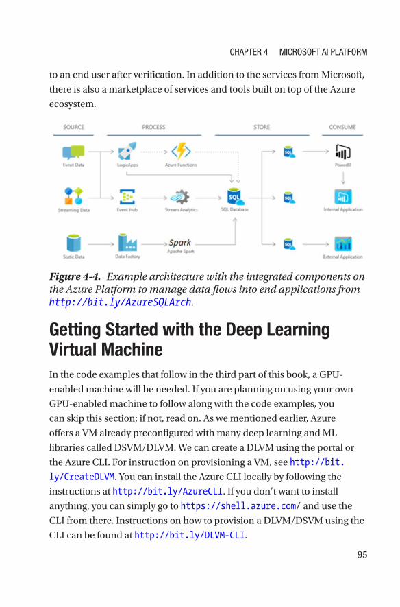
95
to an end user after verification. In addition to the services from Microsoft,
there is also a marketplace of services and tools built on top of the Azure
ecosystem.
Figure 4-4. Example architecture with the integrated components on the Azure Platform to manage data flows into end applications from http://bit.ly/AzureSQLArch.
Getting Started with the Deep Learning Virtual MachineIn the code examples that follow in the third part of this book, a GPU-
enabled machine will be needed. If you are planning on using your own
GPU-enabled machine to follow along with the code examples, you
can skip this section; if not, read on. As we mentioned earlier, Azure
offers a VM already preconfigured with many deep learning and ML
libraries called DSVM/DLVM. We can create a DLVM using the portal or
the Azure CLI. For instruction on provisioning a VM, see http://bit.
ly/CreateDLVM. You can install the Azure CLI locally by following the
instructions at http://bit.ly/AzureCLI. If you don’t want to install
anything, you can simply go to https://shell.azure.com/ and use the
CLI from there. Instructions on how to provision a DLVM/DSVM using the
CLI can be found at http://bit.ly/DLVM-CLI.
Chapter 4 MiCrosoft ai platforM
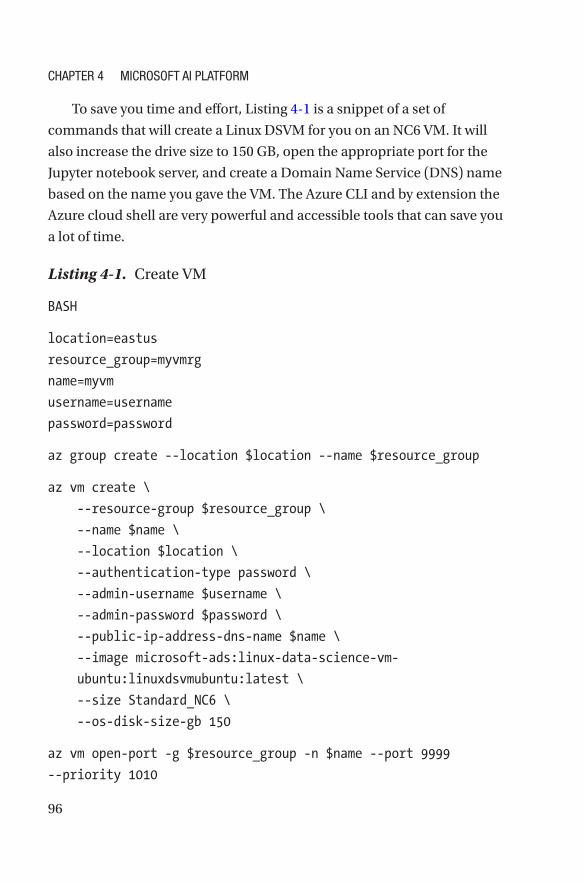
96
To save you time and effort, Listing 4-1 is a snippet of a set of
commands that will create a Linux DSVM for you on an NC6 VM. It will
also increase the drive size to 150 GB, open the appropriate port for the
Jupyter notebook server, and create a Domain Name Service (DNS) name
based on the name you gave the VM. The Azure CLI and by extension the
Azure cloud shell are very powerful and accessible tools that can save you
a lot of time.
Listing 4-1. Create VM
BASH
location=eastus
resource_group=myvmrg
name=myvm
username=username
password=password
az group create --location $location --name $resource_group
az vm create \
--resource-group $resource_group \
--name $name \
--location $location \
--authentication-type password \
--admin-username $username \
--admin-password $password \
--public-ip-address-dns-name $name \
--image microsoft-ads:linux-data-science-vm-
ubuntu:linuxdsvmubuntu:latest \
--size Standard_NC6 \
--os-disk-size-gb 150
az vm open-port -g $resource_group -n $name --port 9999
--priority 1010
Chapter 4 MiCrosoft ai platforM
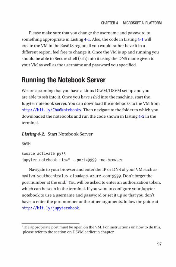
97
Please make sure that you change the username and password to
something appropriate in Listing 4-1. Also, the code in Listing 4-1 will
create the VM in the EastUS region; if you would rather have it in a
different region, feel free to change it. Once the VM is up and running you
should be able to Secure shell (ssh) into it using the DNS name given to
your VM as well as the username and password you specified.
Running the Notebook ServerWe are assuming that you have a Linux DLVM/DSVM set up and you
are able to ssh into it. Once you have ssh’d into the machine, start the
Jupyter notebook server. You can download the notebooks to the VM from
http://bit.ly/Ch06Notebooks. Then navigate to the folder to which you
downloaded the notebooks and run the code shown in Listing 4-2 in the
terminal.
Listing 4-2. Start Notebook Server
BASH
source activate py35
jupyter notebook –ip=* --port=9999 –no-browser
Navigate to your browser and enter the IP or DNS of your VM such as
mydlvm.southcentralus.cloudapp.azure.com:9999. Don’t forget the
port number at the end.1 You will be asked to enter an authorization token,
which can be seen in the terminal. If you want to configure your Jupyter
notebook to use a username and password or set it up so that you don’t
have to enter the port number or the other arguments, follow the guide at
http://bit.ly/jupyternbook.
1 The appropriate port must be open on the VM. For instructions on how to do this, please refer to the section on DSVM earlier in chapter.
Chapter 4 MiCrosoft ai platforM
98
SummaryThis chapter outlined the Microsoft AI Platform set of services, tools, and
infrastructure for building AI solutions. Building AI solutions requires
lots of experimentation and specialized hardware for deep learning, and
leveraging cloud computing combined with service and tools accelerates
the development process of intelligence applications.
Additionally, AI is being infused in other ways across Microsoft’s
products as well, such as on-premises solutions for AI such as SQL Server
2017 and Microsoft Machine Learning Server. SQL Server 2017 runs on
Windows Server, Linux, and Docker and enables advanced in-database
ML with scalable Python and R-based analytics. With SQL Server, models
can be trained within the database without having to move data and
predictions can be made naturally through stored procedures and native
ML functions within the database engine. This capability is included
within Azure SQL DB as well.
In the next chapter, a more detailed overview is available on the
prebuilt AI that is available to infuse directly into applications.
Chapter 4 MiCrosoft ai platforM
99© Mathew Salvaris, Danielle Dean, Wee Hyong Tok 2018 M. Salvaris et al., Deep Learning with Azure, https://doi.org/10.1007/978-1-4842-3679-6_5
CHAPTER 5
Cognitive Services and Custom VisionChapter 4 introduced the tools, infrastructure, and services that are
available to build the next generation of intelligent applications. These
together form a platform that empowers data scientists and developers to
build, train, and deploy ML and deep learning models on the intelligent
cloud and intelligent edge.
As one option within the Microsoft AI Platform, organizations getting
started on AI have the flexibility to use prebuilt AI capabilities using
Cognitive Services. This enables organizations to jump start their AI efforts
quickly and use Cognitive Services as the basis for developing intelligent,
innovative applications. In this chapter, we describe how to use Cognitive
Services. We also illustrate how to customize deep neural network models
for computer vision tasks using the Custom Vision service as one example
of a customizable cognitive service.
Prebuilt AI: Why and How?For years, researchers in the deep learning communities have been making
tremendous progress on algorithms and leveraging state-of-art hardware
to train deep learning models using publicly available large data sets (e.g.,
ImageNet, CIFAR-10, CIFAR-100, Places2, COCO, MegaFace, Switchboard,
and many more). These public data sets are often used in competitions,

100
and as a method for benchmarking for deep learning algorithms. In
addition, many commercial and research organizations leverage private
data sets to further improve the quality of their models.
To train a high-performing deep learning model often requires a
significant amount of computing resources. Chapter 2 described the
amount of computing resources required to train a classifier on ImageNet
(ranging from 256 to 1,024 Nvidia P100 GPUs). Even though training time
has been decreasing significantly over time (from days to minutes), not
every organization has at their disposal a large amount of GPU resources,
nor the means to keep these GPU resources updated with both the latest
hardware and software over time.
Researchers spend a significant amount of time fine-tuning their
models. For example, the accuracy of classifying objects in the ImageNet
data set has improved significantly from 71.8 percent to 97.3 percent
(Russakovsky et al., 2015). Another example is the significant improvement
made by researchers working on speech recognition using the Switchboard
data set. Using a combination of neural-network-driven acoustic and
language models, CNNs, and bidirectional long- and short- term memory
models, Microsoft researchers reduce the error rate for speech recognition to
5.1 percent (Xiong et al., 2016). The deep-learning- based speech recognition
models surpass the performance of professional human transcribers.
Pretrained deep learning models enable organizations to leverage
the significant innovations made by researchers over the years and use
the models immediately to solve common AI problems. For example, we
can leverage speech-to-text APIs that are backed by high-quality speech
models, or computer vision APIs that are trained on large data sets of
faces, scenes, celebrities, and more. These enable organizations to quickly
develop intelligent applications without spending a significant amount of
time training the models.
Chapter 5 Cognitive ServiCeS and CuStom viSion

101
In Chapter 2, we introduce how transfer learning can be applied for
computer vision tasks, where you can leverage pretrained models as
base models and adapt them to new domains by providing new labeled
images. To make it easier for organizations to use custom deep learning
models, Custom Vision (one of the Cognitive Services) enables you to
upload your images and train a custom image classifier quickly with the
press of a few buttons. Similarly, you can customize acoustic models using
Custom Speech (another cognitive service) through uploading domain-
specific data (.wav files, text files, or both) to improve accuracy in various
environments.
More Info Find out more about creating custom acoustic and language model using Custom Speech Service at http://bit.ly/CustomSpeech/.
In this chapter, we focus on computer vision services. We walk through
different types of prebuilt computer vision services that you can use out of
the box. We then describe how to use the Custom Vision Service to train
custom image classifiers.
Cognitive ServicesCognitive Services enables developers to get started quickly by leveraging
prebuilt AI models. To develop an AI application that uses one or more
of the Cognitive Services, developers leverage the APIs provided by each
of the Cognitive Services. This enables developers to develop intelligent
applications using various programming languages (e.g., C#, Java,
JavaScript, PHP, Python, Ruby, etc.).
Figure 5-1 shows how an application interacts with Cognitive Services.
The application issues a request to a Cognitive Services URL. For example,
a Request URL for using Cognitive Services to tag an image (identify what
Chapter 5 Cognitive ServiCeS and CuStom viSion
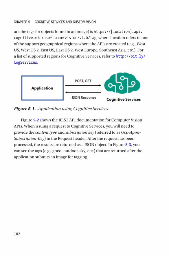
102
are the tags for objects found in an image) is https://[location].api.
cognitive.microsoft.com/vision/v1.0/tag, where location refers to one
of the support geographical regions where the APIs are created (e.g., West
US, West US 2, East US, East US 2, West Europe, Southeast Asia, etc.). For
a list of supported regions for Cognitive Services, refer to http://bit.ly/
CogServices.
Figure 5-1. Application using Cognitive Services
Figure 5-2 shows the REST API documentation for Computer Vision
APIs. When issuing a request to Cognitive Services, you will need to
provide the content type and subscription key (referred to as Ocp-Apim-
Subscription-Key) in the Request header. After the request has been
processed, the results are returned as a JSON object. In Figure 5-3, you
can see the tags (e.g., grass, outdoor, sky, etc.) that are returned after the
application submits an image for tagging.
Chapter 5 Cognitive ServiCeS and CuStom viSion
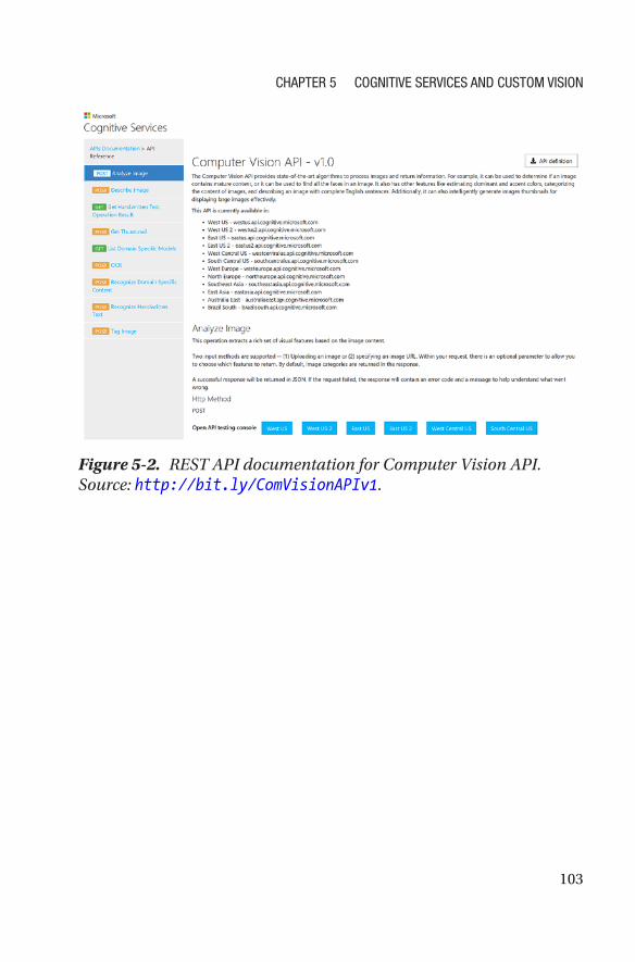
103
Figure 5-2. REST API documentation for Computer Vision API. Source: http://bit.ly/ComVisionAPIv1.
Chapter 5 Cognitive ServiCeS and CuStom viSion
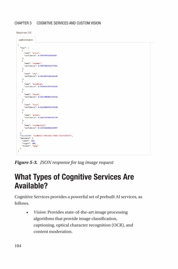
104
What Types of Cognitive Services Are Available?Cognitive Services provides a powerful set of prebuilt AI services, as
follows.
• Vision: Provides state-of-the-art image processing
algorithms that provide image classification,
captioning, optical character recognition (OCR), and
content moderation.
Figure 5-3. JSON response for tag image request
Chapter 5 Cognitive ServiCeS and CuStom viSion

105
• Knowledge: Provides APIs to enable you to quickly
extract question–answer pairs from user-provided
frequently answered questions (FAQs), documents,
and content. Other Knowledge APIs include custom
decision service, knowledge exploration, and named
entity recognition and disambiguation.
• Language: Language Understanding (LUIS) enables
developers to integrate powerful natural language
understanding capabilities into various applications.
Other Language services include Bing Spell Check, Text
Analytics, Translations, and more.
• Speech: Provides APIs for real-time speech translation,
converting speech to text, speaker recognition, and
customizing speech models.
• Search: Provides APIs that provide developers with
instant access to various Bing capabilities. These
include the ability to perform autosuggestion, news
search, web search, image search, video search, and
custom search.
In this chapter, we describe how to use the Computer Vision APIs
that are available as part of Cognitive Services. We refer the interested
reader to continue exploring other Cognitive Services by visiting
http://bit.ly/MSFTCogServices. All Cognitive Services follow a
similar request–response pattern, and you will be able to apply and
adapt what you have learned from using the Computer Vision APIs to
the other Cognitive Services.
Chapter 5 Cognitive ServiCeS and CuStom viSion
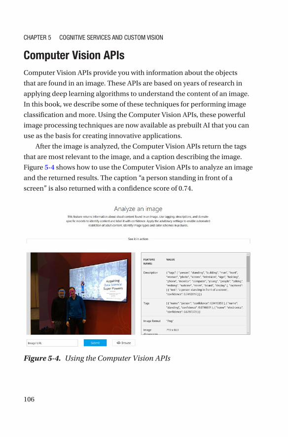
106
Computer Vision APIsComputer Vision APIs provide you with information about the objects
that are found in an image. These APIs are based on years of research in
applying deep learning algorithms to understand the content of an image.
In this book, we describe some of these techniques for performing image
classification and more. Using the Computer Vision APIs, these powerful
image processing techniques are now available as prebuilt AI that you can
use as the basis for creating innovative applications.
After the image is analyzed, the Computer Vision APIs return the tags
that are most relevant to the image, and a caption describing the image.
Figure 5-4 shows how to use the Computer Vision APIs to analyze an image
and the returned results. The caption “a person standing in front of a
screen” is also returned with a confidence score of 0.74.
Figure 5-4. Using the Computer Vision APIs
Chapter 5 Cognitive ServiCeS and CuStom viSion
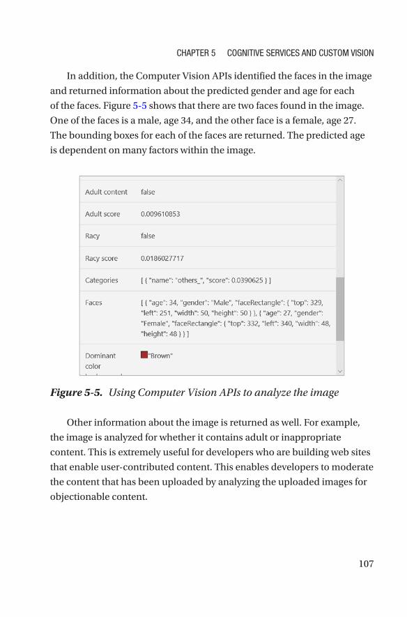
107
In addition, the Computer Vision APIs identified the faces in the image
and returned information about the predicted gender and age for each
of the faces. Figure 5-5 shows that there are two faces found in the image.
One of the faces is a male, age 34, and the other face is a female, age 27.
The bounding boxes for each of the faces are returned. The predicted age
is dependent on many factors within the image.
Figure 5-5. Using Computer Vision APIs to analyze the image
Other information about the image is returned as well. For example,
the image is analyzed for whether it contains adult or inappropriate
content. This is extremely useful for developers who are building web sites
that enable user-contributed content. This enables developers to moderate
the content that has been uploaded by analyzing the uploaded images for
objectionable content.
Chapter 5 Cognitive ServiCeS and CuStom viSion
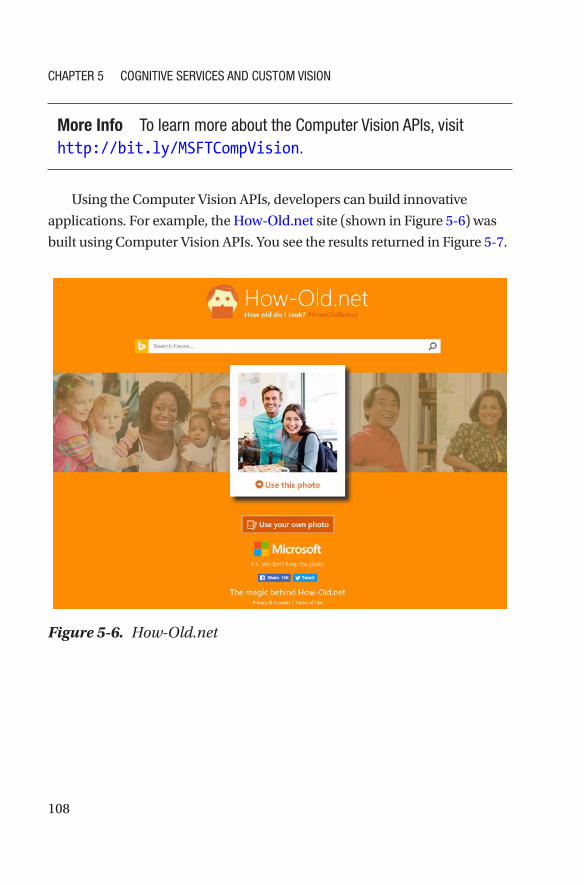
108
More Info to learn more about the Computer vision apis, visit http://bit.ly/MSFTCompVision.
Using the Computer Vision APIs, developers can build innovative
applications. For example, the How-Old.net site (shown in Figure 5-6) was
built using Computer Vision APIs. You see the results returned in Figure 5- 7.
Figure 5-6. How-Old.net
Chapter 5 Cognitive ServiCeS and CuStom viSion
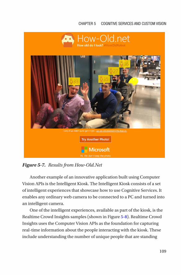
109
Another example of an innovative application built using Computer
Vision APIs is the Intelligent Kiosk. The Intelligent Kiosk consists of a set
of intelligent experiences that showcase how to use Cognitive Services. It
enables any ordinary web camera to be connected to a PC and turned into
an intelligent camera.
One of the intelligent experiences, available as part of the kiosk, is the
Realtime Crowd Insights samples (shown in Figure 5-8). Realtime Crowd
Insights uses the Computer Vision APIs as the foundation for capturing
real-time information about the people interacting with the kiosk. These
include understanding the number of unique people that are standing
Figure 5-7. Results from How-Old.Net
Chapter 5 Cognitive ServiCeS and CuStom viSion

110
in front of the kiosk, counting of unique faces, and looking at the overall
emotions. This sample provides the basis for developing interactive
and intelligent experiences for kiosks that are deployed in retail malls
and more.
Figure 5-8. Intelligent Kiosk Realtime Crowd Insights
More Info the code for intelligent Kiosk is open source and is available at http://bit.ly/IntelligentKiosk.
How to Use Optical Character Recognition–
The Computer Vision APIs enable you to perform OCR for printed and
handwritten text. To do this, you can upload an image or provide the
URL where the image is stored. The APIs will detect the text in the image
and return in a JSON payload the characters that are recognized. Various
Chapter 5 Cognitive ServiCeS and CuStom viSion
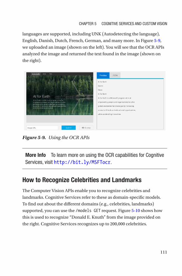
111
languages are supported, including UNK (Autodetecting the language),
English, Danish, Dutch, French, German, and many more. In Figure 5-9,
we uploaded an image (shown on the left). You will see that the OCR APIs
analyzed the image and returned the text found in the image (shown on
the right).
Figure 5-9. Using the OCR APIs
More Info to learn more on using the oCr capabilities for Cognitive Services, visit http://bit.ly/MSFTocr.
How to Recognize Celebrities and Landmarks
The Computer Vision APIs enable you to recognize celebrities and
landmarks. Cognitive Services refer to these as domain-specific models.
To find out about the different domains (e.g., celebrities, landmarks)
supported, you can use the /models GET request. Figure 5-10 shows how
this is used to recognize “Donald E. Knuth” from the image provided on
the right. Cognitive Services recognizes up to 200,000 celebrities.
Chapter 5 Cognitive ServiCeS and CuStom viSion
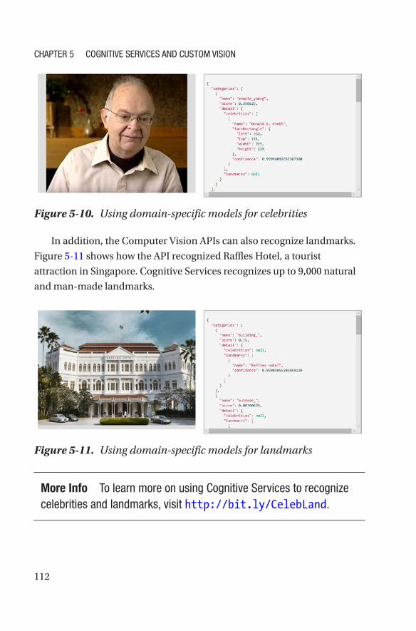
112
In addition, the Computer Vision APIs can also recognize landmarks.
Figure 5-11 shows how the API recognized Raffles Hotel, a tourist
attraction in Singapore. Cognitive Services recognizes up to 9,000 natural
and man-made landmarks.
Figure 5-10. Using domain-specific models for celebrities
Figure 5-11. Using domain-specific models for landmarks
More Info to learn more on using Cognitive Services to recognize celebrities and landmarks, visit http://bit.ly/CelebLand.
Chapter 5 Cognitive ServiCeS and CuStom viSion
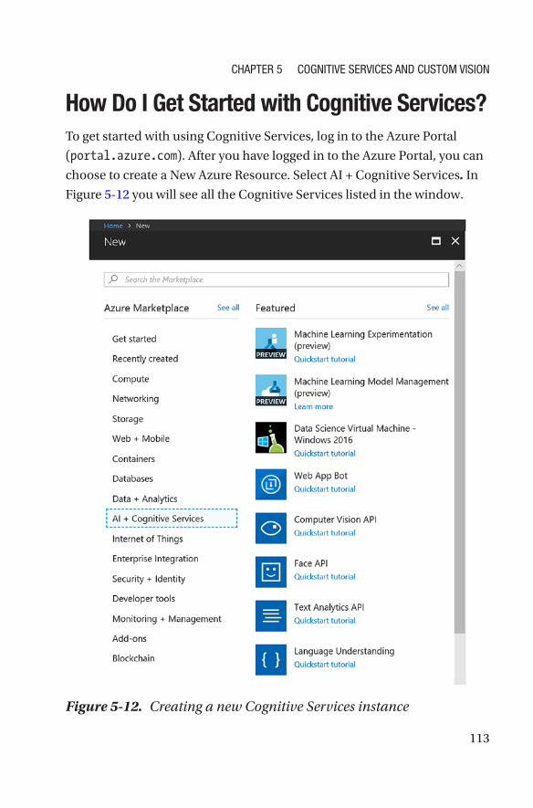
113
How Do I Get Started with Cognitive Services?To get started with using Cognitive Services, log in to the Azure Portal
(portal.azure.com). After you have logged in to the Azure Portal, you can
choose to create a New Azure Resource. Select AI + Cognitive Services. In
Figure 5-12 you will see all the Cognitive Services listed in the window.
Figure 5-12. Creating a new Cognitive Services instance
Chapter 5 Cognitive ServiCeS and CuStom viSion
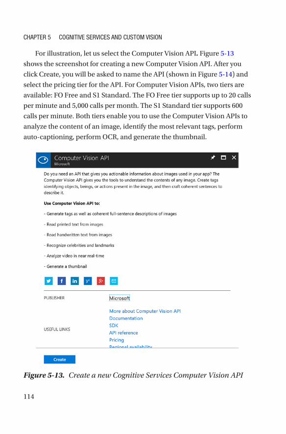
114
For illustration, let us select the Computer Vision API. Figure 5-13
shows the screenshot for creating a new Computer Vision API. After you
click Create, you will be asked to name the API (shown in Figure 5-14) and
select the pricing tier for the API. For Computer Vision APIs, two tiers are
available: FO Free and S1 Standard. The FO Free tier supports up to 20 calls
per minute and 5,000 calls per month. The S1 Standard tier supports 600
calls per minute. Both tiers enable you to use the Computer Vision APIs to
analyze the content of an image, identify the most relevant tags, perform
auto-captioning, perform OCR, and generate the thumbnail.
Figure 5-13. Create a new Cognitive Services Computer Vision API
Chapter 5 Cognitive ServiCeS and CuStom viSion
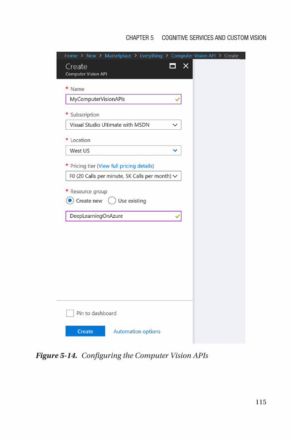
115
Figure 5-14. Configuring the Computer Vision APIs
Chapter 5 Cognitive ServiCeS and CuStom viSion

116
After the Computer Vision API has been created, you can manage it
using the Azure Portal. Figure 5-15 shows how you can manage the newly
created Computer Vision API. To use the API in your application, you
will need to specify the API key. You can click Keys in the management
window, which will show you the keys that are available. Figure 5-16
shows the two keys that are available. You can make use of the Primary
and Secondary key during key rotation. You can use either of the keys in
your application. This is specified as part of the Request header. If you
are developing a .NET application to use Cognitive Services, the key is
specified as part of the API call. Listing 5-1 shows the sample code for
accessing the Computer Vision APIs. For example, you should replace the
"{subscription key}" placeholder in the code with the subscription key
that you obtained from the Azure Portal.
Figure 5-15. Managing Cognitive Services
Chapter 5 Cognitive ServiCeS and CuStom viSion
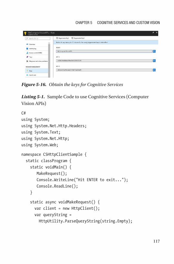
117
Listing 5-1. Sample Code to use Cognitive Services (Computer
Vision APIs)
C#
using System;
using System.Net.Http.Headers;
using System.Text;
using System.Net.Http;
using System.Web;
namespace CSHttpClientSample {
static classProgram {
static voidMain() {
MakeRequest();
Console.WriteLine("Hit ENTER to exit...");
Console.ReadLine();
}
static async voidMakeRequest() {
var client = new HttpClient();
var queryString =
HttpUtility.ParseQueryString(string.Empty);
Figure 5-16. Obtain the keys for Cognitive Services
Chapter 5 Cognitive ServiCeS and CuStom viSion
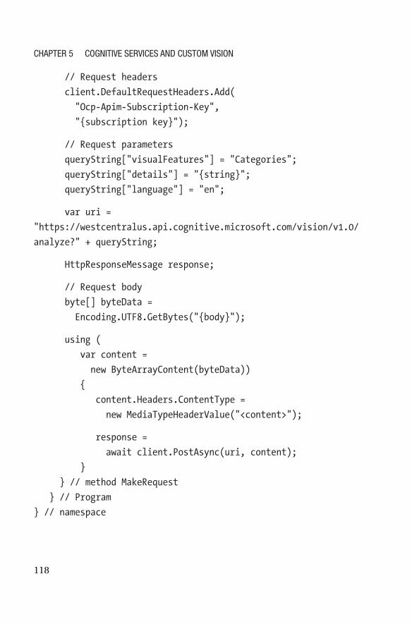
118
// Request headers
client.DefaultRequestHeaders.Add(
"Ocp-Apim-Subscription-Key",
"{subscription key}");
// Request parameters
queryString["visualFeatures"] = "Categories";
queryString["details"] = "{string}";
queryString["language"] = "en";
var uri =
"https://westcentralus.api.cognitive.microsoft.com/vision/v1.0/
analyze?" + queryString;
HttpResponseMessage response;
// Request body
byte[] byteData =
Encoding.UTF8.GetBytes("{body}");
using (
var content =
new ByteArrayContent(byteData))
{
content.Headers.ContentType =
new MediaTypeHeaderValue("<content>");
response =
await client.PostAsync(uri, content);
}
} // method MakeRequest
} // Program
} // namespace
Chapter 5 Cognitive ServiCeS and CuStom viSion
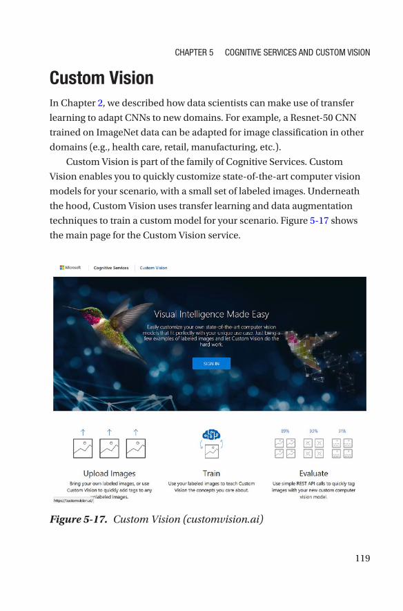
119
Figure 5-17. Custom Vision (customvision.ai)
Custom VisionIn Chapter 2, we described how data scientists can make use of transfer
learning to adapt CNNs to new domains. For example, a Resnet-50 CNN
trained on ImageNet data can be adapted for image classification in other
domains (e.g., health care, retail, manufacturing, etc.).
Custom Vision is part of the family of Cognitive Services. Custom
Vision enables you to quickly customize state-of-the-art computer vision
models for your scenario, with a small set of labeled images. Underneath
the hood, Custom Vision uses transfer learning and data augmentation
techniques to train a custom model for your scenario. Figure 5-17 shows
the main page for the Custom Vision service.
Chapter 5 Cognitive ServiCeS and CuStom viSion

120
More Info did you know that you can use Custom vision programmatically? using C# or python, you can programmatically create a Custom vision project, add tags, upload images, and train the project. after the custom vision models are trained, you can retrieve the prediction urL and test the custom image classifier. to find out more, visit http://bit.ly/CustomVisionProg.
Hello World! for Custom VisionIn this section, we will learn how to get started with Custom Vision. On
the customvision.ai page, click Sign In. During the first sign in to Custom
Vision, you will need to accept the terms of use. You will be prompted to
indicate whether you want to use an Azure account, which will enable you
to work with more Custom Vision projects. If you do not sign in to Azure,
you will have access to fewer quotas. Figure 5-18 shows the initial page
after you sign in. If you do not have an Azure subscription, you can click I’ll
Do It Later.
Chapter 5 Cognitive ServiCeS and CuStom viSion

121
After you sign in, you can create your first Custom Vision project by
clicking New Project. As shown in Figure 5-19, we create our first Hello
World Custom Vision project. Several domains are provided that will
enable you to customize the base model that is most relevant to your
scenario. In this example, we selected General (Compact). Compact
domains enable you to export the trained models, which we cover in a
later section.
Figure 5-18. Custom Vision first sign in
Chapter 5 Cognitive ServiCeS and CuStom viSion
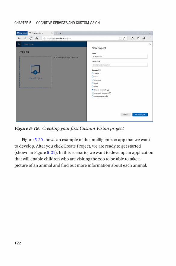
122
Figure 5-20 shows an example of the intelligent zoo app that we want
to develop. After you click Create Project, we are ready to get started
(shown in Figure 5-21). In this scenario, we want to develop an application
that will enable children who are visiting the zoo to be able to take a
picture of an animal and find out more information about each animal.
Figure 5-19. Creating your first Custom Vision project
Chapter 5 Cognitive ServiCeS and CuStom viSion
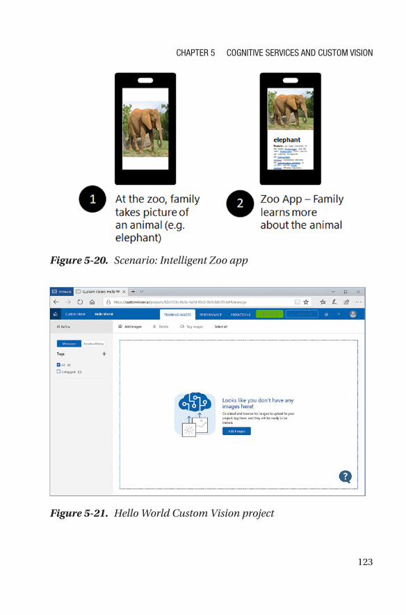
123
Figure 5-20. Scenario: Intelligent Zoo app
Figure 5-21. Hello World Custom Vision project
Chapter 5 Cognitive ServiCeS and CuStom viSion
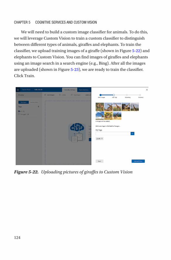
124
Figure 5-22. Uploading pictures of giraffes to Custom Vision
We will need to build a custom image classifier for animals. To do this,
we will leverage Custom Vision to train a custom classifier to distinguish
between different types of animals, giraffes and elephants. To train the
classifier, we upload training images of a giraffe (shown in Figure 5-22) and
elephants to Custom Vision. You can find images of giraffes and elephants
using an image search in a search engine (e.g., Bing). After all the images
are uploaded (shown in Figure 5-23), we are ready to train the classifier.
Click Train.
Chapter 5 Cognitive ServiCeS and CuStom viSion
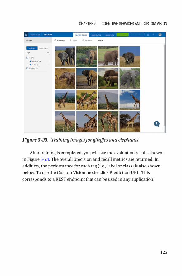
125
Figure 5-23. Training images for giraffes and elephants
After training is completed, you will see the evaluation results shown
in Figure 5-24. The overall precision and recall metrics are returned. In
addition, the performance for each tag (i.e., label or class) is also shown
below. To use the Custom Vision mode, click Prediction URL. This
corresponds to a REST endpoint that can be used in any application.
Chapter 5 Cognitive ServiCeS and CuStom viSion
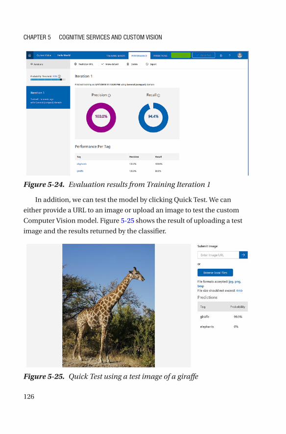
126
In addition, we can test the model by clicking Quick Test. We can
either provide a URL to an image or upload an image to test the custom
Computer Vision model. Figure 5-25 shows the result of uploading a test
image and the results returned by the classifier.
Figure 5-24. Evaluation results from Training Iteration 1
Figure 5-25. Quick Test using a test image of a giraffe
Chapter 5 Cognitive ServiCeS and CuStom viSion
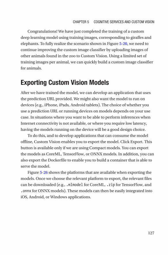
127
Congratulations! We have just completed the training of a custom
deep learning model using training images, corresponding to giraffes and
elephants. To fully realize the scenario shown in Figure 5-20, we need to
continue improving the custom image classifier by uploading images of
other animals found in the zoo to Custom Vision. Using a limited set of
training images per animal, we can quickly build a custom image classifier
for animals.
Exporting Custom Vision ModelsAfter we have trained the model, we can develop an application that uses
the prediction URL provided. We might also want the model to run on
devices (e.g., iPhone, iPads, Android tablets). The choice of whether you
use a prediction URL or running devices on models depends on your use
case. In situations where you want to be able to perform inferences when
Internet connectivity is not available, or where you require low latency,
having the models running on the device will be a good design choice.
To do this, and to develop applications that can consume the model
offline, Custom Vision enables you to export the model. Click Export. This
button is available only if we are using Compact models. You can export
the models as CoreML, TensorFlow, or ONNX models. In addition, you can
also export the Dockerfile to enable you to build a container that is able to
serve the model.
Figure 5-26 shows the platforms that are available when exporting the
models. Once we choose the relevant platform to export, the relevant files
can be downloaded (e.g., .mlmodel for CoreML, .zip for TensorFlow, and
.onnx for ONNX models). These models can then be easily integrated into
iOS, Android, or Windows applications.
Chapter 5 Cognitive ServiCeS and CuStom viSion

128
SummaryThis chapter discussed the different types of Cognitive Services that are
available as part of the Microsoft AI Platform. These prebuilt AI capabilities
enable developers in your organization to get started immediately with
realizing the value of AI to develop innovative applications. In addition, we
also illustrated how to adapt pretrained deep learning models for computer
vision to new data using Custom Vision. This enables you to quickly train
an image classification model by bringing your own data. To enable you to
do AI on the intelligent edge (IoT edge device, iOS and Android devices),
Custom Vision enables you to explore CoreML and TensorFlow models. This
chapter only touched the surface of the different Cognitive Services available
on the Microsoft AI Platform. We encourage you to explore others in more
depth as well, such the Language Understanding service, Azure Search, and
Custom Speech service, depending on your use case and needs.
In the next set of chapters, rather than focus on using prebuilt AI
capabilities as discussed here, we instead focus on an overview of how to
build custom deep learning models, starting with an overview of common
models such as CNNs in the next chapter.
Figure 5-26. Exporting Custom Vision models to CoreML or TensorFlow
Chapter 5 Cognitive ServiCeS and CuStom viSion

PART III
AI Networks in Practice

131© Mathew Salvaris, Danielle Dean, Wee Hyong Tok 2018 M. Salvaris et al., Deep Learning with Azure, https://doi.org/10.1007/978-1-4842-3679-6_6
CHAPTER 6
Convolutional Neural NetworksCNNs are a prime example of neuroscience influencing deep learning
(LeCun, Bottou, Bengio, & Haffner, 1998). These neural networks are based
on the seminal work done by Hubel and Wiesel (1962). They discovered
that individual neuronal cells in the visual cortex responded only to the
presence of visual features such as edges of certain orientations. From their
experiments they deduced that the visual cortex contains a hierarchical
arrangement of neuronal cells. These neurons are sensitive to specific
subregions in the visual field, with these subregions being tiled to cover
the entire visual field. They in fact act as localized filters over the input
space, making them well suited to exploiting the strong spatial correlation
found in natural images. CNNs have been immensely successful in many
computer vision tasks not just because of the inspiration drawn from
neuroscience, but also due to the clever engineering principles employed.
Although they have traditionally been used for applications in the field of
computer vision such as face recognition and image classification, CNNs
have also been used in other areas such as speech recognition and natural
language processing for certain tasks.
This chapter briefly describes what convolution is and how it relates
to neural networks. It then explains the various elements that make up
the CNN architecture and what effects they have, and why CNNs do so
well. Finally, it covers the usual steps to training CNNs before diving into a
132
number of practical examples, using the CIFAR10 data set to train a CNN
using Jupyter notebooks.
One of the first successful applications of CNNs was in the 1990s,
reading zip codes using the LeNet architecture from Yann LeCun and
colleagues (LeCun, Boser, et al., 1989). However, CNNs were widely
popularized in 2012 with the AlexNet (Krizhevsky, Sutskever, & Hinton,
2012) architecture, which won the ImageNet Large Scale Visual
Recognition Competition (ILSVRC) as mentioned in Chapter 1 and led
to a breakthrough in the computer vision field. Since then, there have
been many useful developments and recommended architectures from
researchers such as VGGNet (Simonyan & Zisserman, 2014) and ResNet
(He, Zhang, Ren, & Sun, 2016). We do not recommend a specific neural
network architecture because this is still a fast-moving field with new
breakthroughs happening frequently. Instead, we recommend that
practitioners pick out an architecture already available that has been
developed and tested by researchers, and if necessary tweak it.
The Convolution in Convolution Neural NetworksTo keep things simple when talking about convolution we will be
talking about discrete convolution. Mathematically, convolution is the
simple summation of the pointwise multiplication of two functions. The
summations can take place in one or more dimensions, so for grayscale
images the summation would take place over two dimensions and over
three dimensions in color images.
Convolution is similar to cross-correlation and in many deep learning
libraries the implementation is actually cross-correlation even though it
is referred to as convolution. For all practical purposes in the CNNs this
is just an implementation detail and does not really affect the resulting
behavior of the model. To get an intuitive feeling of how convolution
behaves, there is a simple example illustrated in Figure 6-1.
Chapter 6 Convolutional neural networks

133
In this example the image is represented by a 5 × 5 matrix and each
pixel can only take on two values, 1 or 0. We have a convolution kernel
that detects diagonal lines. Convolution kernels are sometimes referred
to as filters or feature detectors. By convolving our kernel with the image
we get our feature and activation map. The top left value of our feature
map is created by multiplying all the values in the overlapping matrices
and then summing the result. In the bottom row of the image we can see
that applying the kernel to our image we get a value of three. The kernel
is applied to the nine pixels in the top left area of our image. If we were to
flatten out the values row wise we would have the vector [1,1,1,0,1,1,0,1,1].
The kernel would correspond to the vector [1,0,0,0,1,0,0,0,1]. If we multiply
the two vectors element wise as so [ 1*1, 1*0, 1*0, 0*0 …] we will end up
with the vector [1,0,0,0,1,0,0,0,1], which we sum to get the value 3. In
essence we are computing the dot product of the two vectors to end up
with a scalar value.
Figure 6-1. Convolution in CNNs
Chapter 6 Convolutional neural networks

134
We then shift the kernel right by one—this is often referred to as the
stride—and do the same thing again. Notice that the feature map is smaller
than the original image. To mitigate this, CNNs often employ padding
of the input image so that the resulting feature map does not reduce in
size, as this constant reduction would limit the number of successive
convolutions that could be applied. This is just a simple example, as real
color images have three color channels—red, green, and blue—and the
pixel value of each channel is represented by an integer between 0 and
255. For a single image, our input would be a three-dimensional matrix
with the width, height, and number of channels. Depending on the deep
learning framework you use, some expect the channels to be first CHW or
channels to be last HWC.
Convolution LayerCNNs employ convolution in what are referred to as convolution layers,
which are simply a number of convolution kernels represented by the
weights of each convolution layer. The dimensions and stride of the
convolution are usually predefined, but the weights are learned as the
network is trained. A CNN will typically have many convolution layers and
each convolution layer will have its own set of learned kernels or filters.
Figure 6-2 is a selection of convolution filters taken from a pretrained
CNN. The top row is of six filters from the first convolution layer. The
bottom row is from the last convolution layer in the CNN. Going from the
top to the bottom, it looks like the convolution layers are looking at ever
more complex patterns. The first layer is encoding direction and color.
The second layer seems to be more interested in spot and grid textures.
The final layer looks like a complex combination of various textures. From
this we can see that as we go through the network the patterns become
more intricate, so the deeper the network the more complex patterns the
convolution layers will learn to extract.
Chapter 6 Convolutional neural networks

135
Another interesting thing to note is that if we look at the first and
last filter on the middle row it seems like they could be slightly rotated
variations of the same filter. This highlights one of the deficiencies of
CNNs: They are not rotation invariant. This is something Hinton has tried
to overcome with capsule networks, as discussed in Chapter 3.
Pooling LayerConvolution is not equivariant, meaning that on their own they do not deal
well with scaling and rotation of the input (Sabour, Frosst, & Hinton, 2017).
A common type of layer in modern CNNs to help deal with this is a pooling
layer, with the most popular pooling layer being the max pooling layer.
Max pooling replaces the output of spatially adjacent outputs with the max
of those values. Generally pooling layers replace the outputs with some
form of summary statistic based on those outputs.
Figure 6-2. Visualization of convolution layers. For more detailed visualizations take a look at Zeiler and Fergus (2013).
Chapter 6 Convolutional neural networks

136
Generally, the pooling layer’s purpose is to make neural networks
locally invariant to small translations of the input, and its essence to care
more about whether a feature is detected rather than where exactly it is in
the input. This does, in turn, reduce the spatial acuity of the model and is
considered a limitation of CNNs; however, pooling layers have proven to
be extremely useful.
Activation FunctionsActivation functions are very important in CNNs and artificial neural networks
in general. Without them CNNs would simply be a series of linear operations
and would not be able to do the amazing things they do today. Activation
functions are simply nonlinear transformations of the output of a neuron in
a layer. They are referred to as activation functions because they draw their
inspiration from the threshold and fire activation of biological neurons.
There are a number of different activation functions with different properties
and specialization, but we go over only the most common types here.
Sigmoid
Sigmoid or logistic is a nonlinear function, which squashes the input
between the values of 0 and 1 (Figure 6-3).
f xe x( ) =
+ -
1
1
Chapter 6 Convolutional neural networks
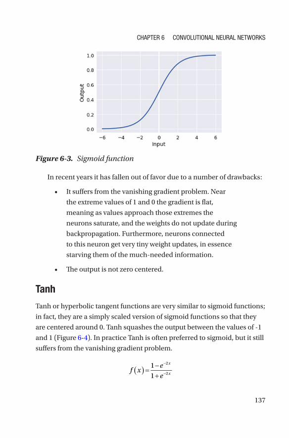
137
In recent years it has fallen out of favor due to a number of drawbacks:
• It suffers from the vanishing gradient problem. Near
the extreme values of 1 and 0 the gradient is flat,
meaning as values approach those extremes the
neurons saturate, and the weights do not update during
backpropagation. Furthermore, neurons connected
to this neuron get very tiny weight updates, in essence
starving them of the much-needed information.
• The output is not zero centered.
Tanh
Tanh or hyperbolic tangent functions are very similar to sigmoid functions;
in fact, they are a simply scaled version of sigmoid functions so that they
are centered around 0. Tanh squashes the output between the values of -1
and 1 (Figure 6-4). In practice Tanh is often preferred to sigmoid, but it still
suffers from the vanishing gradient problem.
f xx
x( ) = -+
-
-
1
1
2
2
e
e
Figure 6-3. Sigmoid function
Chapter 6 Convolutional neural networks

138
Rectified Linear Unit
The rectified linear unit (ReLU; see Figure 6-5) is probably the most used
activation function nowadays (LeCun, Bengio, & Hinton, 2015).
f x x( ) = ( )max 0,
Figure 6-4. Tanh
Figure 6-5. Rectified linear unit (ReLU)
Chapter 6 Convolutional neural networks
139
With the ReLU activation function, when the input is greater than zero,
then output is the same as the input; when it is less than zero, the output
is zero. Its popularity is mainly due to a couple of facts. First, it does not
saturate or suffer from the vanishing gradient problem in the positive
region. Second, it is a computationally efficient function and it also leads
to sparse activations that also confer computational benefits. It does still
suffer from a couple of drawbacks though:
• If the output of the function is less than zero during
the forward pass, no gradient is propagated backward
during the backward pass. This means that weights
do not get updated. If neurons in the CNN exhibit this
behavior consistently, the neurons are said to be dead,
which means they no longer contribute to the network
and are in essence useless. If this happens to a significant
portion of your CNN, it will stall and fail to learn.
• For classification tasks, it cannot be used in the output
layer because its output isn’t constrained between well-
defined boundaries.
CNN ArchitectureCNNs are typically constructed by stacking multiple layers on top of each
other (Figure 6-6). A common configuration is the following: First, there
is a convolution layer where multiple kernels convolve the input and
produce a number of feature maps. These then pass through a nonlinear
activation function such as ReLU, which is then followed by a pooling
layer. These three stages are often combined in various ways to create the
first few layers of a CNN. The output of the final layer is flattened and then
fed through one or more fully connected layers. The activation function
of the final layer is usually a softmax or sigmoid that squashes the output
between 0 and 1.
Chapter 6 Convolutional neural networks
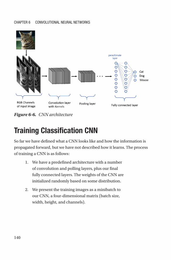
140
Training Classification CNNSo far we have defined what a CNN looks like and how the information is
propagated forward, but we have not described how it learns. The process
of training a CNN is as follows:
1. We have a predefined architecture with a number
of convolution and polling layers, plus our final
fully connected layers. The weights of the CNN are
initialized randomly based on some distribution.
2. We present the training images as a minibatch to
our CNN, a four- dimensional matrix (batch size,
width, height, and channels).
Figure 6-6. CNN architecture
Chapter 6 Convolutional neural networks
141
3. We complete a forward pass through the
networks with the images being passed through
the convolution, pooling layers, and activation
functions, and finally we get the output probabilities
for each class for each image in the minibatch.
4. We compare the probabilities to the true labels and
calculate the error.
5. We use backpropagation to calculate the gradients
of the error with respect to the weights of the CNN
and we use gradient descent to update the weights.
6. This process is repeated either for a set of epochs1 or
until other conditions are met.
This is a simplified view of what happens, but it captures the core of
what it takes to train a CNN, an objective function, a method to calculate
the gradients, and an optimization method.
The objective or loss function determines how we will calculate the
difference between what we expected the network to do and what it did.
In essence it will calculate the error for our model. Common loss functions
are mean squared error (MSE) and cross-entropy. Now once we have the
error, we need to update the weights of the network in the right direction
so that our predictions become a little better next time. This is done by a
method called backpropagation.
The optimization method most commonly used by CNNs is minibatch
gradient descent, often referred to as stochastic gradient descent (SGD),
even though SGD is slightly different from minibatch gradient descent.
Minibatch gradient descent seeks to optimize the objective function by
iteratively updating the weights of the CNN based on the gradients in
each minibatch. Due to the nonlinearities in CNNs, the solution space is
1 Epoch refers to the CNN having seen the whole training set.
Chapter 6 Convolutional neural networks
142
often nonconvex and therefore there are no guarantees of convergence.
For practitioners this can be quite frustrating, but CNNs work surprisingly
well even without this guarantee. The main parameter in all variants of
gradient descent is the learning rate, which determines the magnitude of
the updates applied to the weight of the network. A variant of SGD also
includes a momentum term that tries to accelerate learning by preserving
the direction of travel through the parameter space. It does this by adding a
fraction of the weight update of the previous time step to the current update.
Other optimization algorithms include Adam, RMSProp, and so on.
Why CNNsAs mentioned earlier, CNNs were inspired by neuroscience but they also
make use of sound engineering principles that also confer advantages.
These are sparse connectivity and parameter sharing. Current research
indicates neurons also share these features. A typical human neuron has
7,000 connections (cf. 1011 neurons in the brain). Similarly, each neuronal
cell type shares specific functional parameters. A great example of the latter
are retinal ganglion cells, which all implement effectively the same type
of convolutional kernel (opposing center-surround). The weights of these
kernels were “learned” through evolution of gene expression patterns.
In traditional neural networks such as multilayer perceptrons (MLPs),
every layer is fully connected to every single node of the next layer. As you
increase the number of layers and the number of nodes, the number of
parameters explodes. In CNNs the connections are usually much smaller
than the input because the kernel is convolved over the input, which is
represented by the previous layer. Therefore in an image that is made of
thousands of pixels, the convolution kernel can be just a few tens of pixels.
This reduction in parameters improves the efficiency of the model both in
terms of memory and also in terms of computation due to the reduction in
the amount of computation required.
Chapter 6 Convolutional neural networks

143
The second benefit is parameter sharing. In standard neural networks,
the input weights for each node in the next layer are only used for that
node, whereas in CNNs the same kernel is used many times. Therefore,
instead of learning different parameters for each node, we learn a set of
kernels for all the nodes.
Training CNN on CIFAR10In this next section, we go step by step in training a CNN on the CIFAR10
data set (Krizhevsky 2009; Krizhevsky, Nair, & Hinton, n.d.). We use
TensorFlow as the deep learning library to build our CNN with. The CIFAR102
data set is an often used data set that in total contains 60,000 32 × 32
color images across 10 classes (see Figure 6-7). These are split into 50,000
training and 10,000 test. The code for this section can also be found in the
notebook Chapter_06_01.ipynb (http://bit.ly/Nbook_ch06_01).
More Info we recommend provisioning an azure DlvM to run the code examples in this chapter. please see the Chapter 4 for more information.
2 CIFAR stands for the Canadian Institute for Advanced Research. They are partly responsible for funding Hinton and LeCun during the neural network winter, leading to the eventual resurgence of neural networks as deep learning.
Chapter 6 Convolutional neural networks
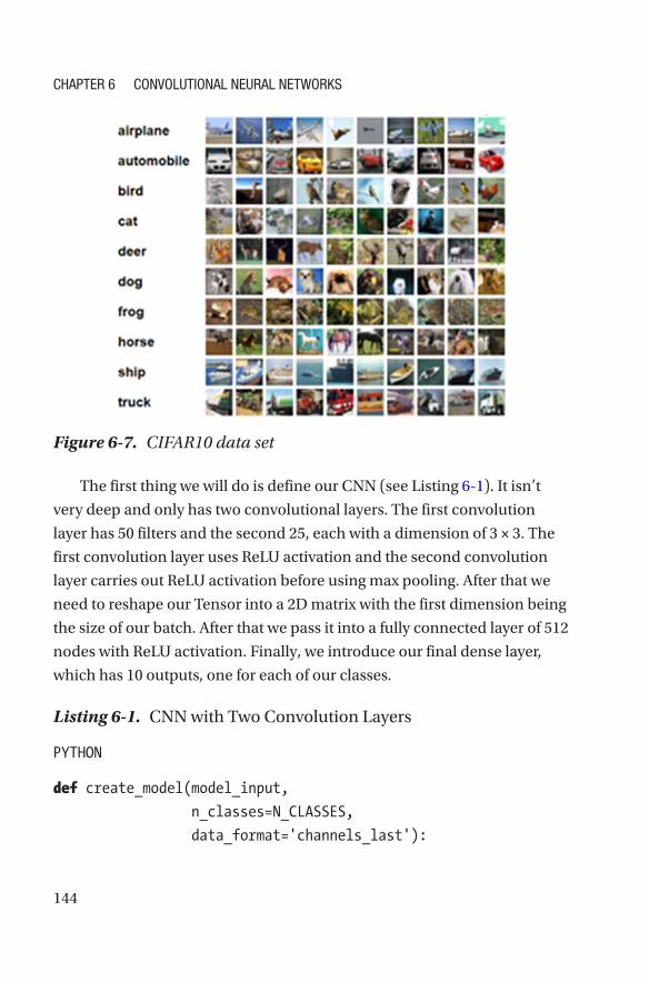
144
The first thing we will do is define our CNN (see Listing 6-1). It isn’t
very deep and only has two convolutional layers. The first convolution
layer has 50 filters and the second 25, each with a dimension of 3 × 3. The
first convolution layer uses ReLU activation and the second convolution
layer carries out ReLU activation before using max pooling. After that we
need to reshape our Tensor into a 2D matrix with the first dimension being
the size of our batch. After that we pass it into a fully connected layer of 512
nodes with ReLU activation. Finally, we introduce our final dense layer,
which has 10 outputs, one for each of our classes.
Listing 6-1. CNN with Two Convolution Layers
PYTHON
def create_model(model_input,
n_classes=N_CLASSES,
data_format='channels_last'):
Figure 6-7. CIFAR10 data set
Chapter 6 Convolutional neural networks
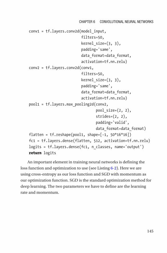
145
conv1 = tf.layers.conv2d(model_input,
filters=50,
kernel_size=(3, 3),
padding='same',
data_format=data_format,
activation=tf.nn.relu)
conv2 = tf.layers.conv2d(conv1,
filters=50,
kernel_size=(3, 3),
padding='same',
data_format=data_format,
activation=tf.nn.relu)
pool1 = tf.layers.max_pooling2d(conv2,
pool_size=(2, 2),
strides=(2, 2),
padding='valid',
data_format=data_format)
flatten = tf.reshape(pool1, shape=[-1, 50*16*16])
fc1 = tf.layers.dense(flatten, 512, activation=tf.nn.relu)
logits = tf.layers.dense(fc1, n_classes, name='output')
return logits
An important element in training neural networks is defining the
loss function and optimization to use (see Listing 6-2). Here we are
using cross-entropy as our loss function and SGD with momentum as
our optimization function. SGD is the standard optimization method for
deep learning. The two parameters we have to define are the learning
rate and momentum.
Chapter 6 Convolutional neural networks
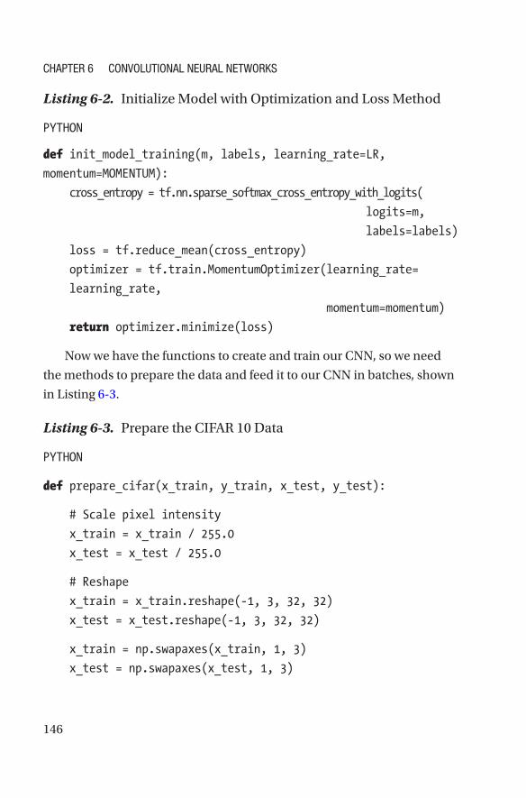
146
Listing 6-2. Initialize Model with Optimization and Loss Method
PYTHON
def init_model_training(m, labels, learning_rate=LR,
momentum=MOMENTUM):
cross_entropy = tf.nn.sparse_softmax_cross_entropy_with_logits(
logits=m,
labels=labels)
loss = tf.reduce_mean(cross_entropy)
optimizer = tf.train.MomentumOptimizer(learning_rate=
learning_rate,
momentum=momentum)
return optimizer.minimize(loss)
Now we have the functions to create and train our CNN, so we need
the methods to prepare the data and feed it to our CNN in batches, shown
in Listing 6-3.
Listing 6-3. Prepare the CIFAR 10 Data
PYTHON
def prepare_cifar(x_train, y_train, x_test, y_test):
# Scale pixel intensity
x_train = x_train / 255.0
x_test = x_test / 255.0
# Reshape
x_train = x_train.reshape(-1, 3, 32, 32)
x_test = x_test.reshape(-1, 3, 32, 32)
x_train = np.swapaxes(x_train, 1, 3)
x_test = np.swapaxes(x_test, 1, 3)
Chapter 6 Convolutional neural networks
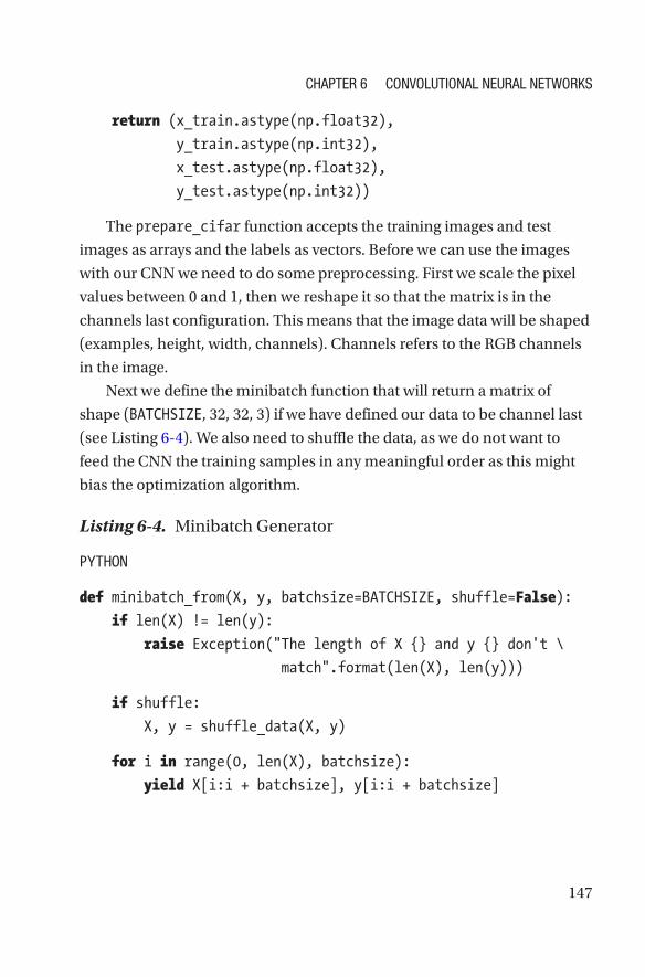
147
return (x_train.astype(np.float32),
y_train.astype(np.int32),
x_test.astype(np.float32),
y_test.astype(np.int32))
The prepare_cifar function accepts the training images and test
images as arrays and the labels as vectors. Before we can use the images
with our CNN we need to do some preprocessing. First we scale the pixel
values between 0 and 1, then we reshape it so that the matrix is in the
channels last configuration. This means that the image data will be shaped
(examples, height, width, channels). Channels refers to the RGB channels
in the image.
Next we define the minibatch function that will return a matrix of
shape (BATCHSIZE, 32, 32, 3) if we have defined our data to be channel last
(see Listing 6-4). We also need to shuffle the data, as we do not want to
feed the CNN the training samples in any meaningful order as this might
bias the optimization algorithm.
Listing 6-4. Minibatch Generator
PYTHON
def minibatch_from(X, y, batchsize=BATCHSIZE, shuffle=False):
if len(X) != len(y):
raise Exception("The length of X {} and y {} don't \
match".format(len(X), len(y)))
if shuffle:
X, y = shuffle_data(X, y)
for i in range(0, len(X), batchsize):
yield X[i:i + batchsize], y[i:i + batchsize]
Chapter 6 Convolutional neural networks
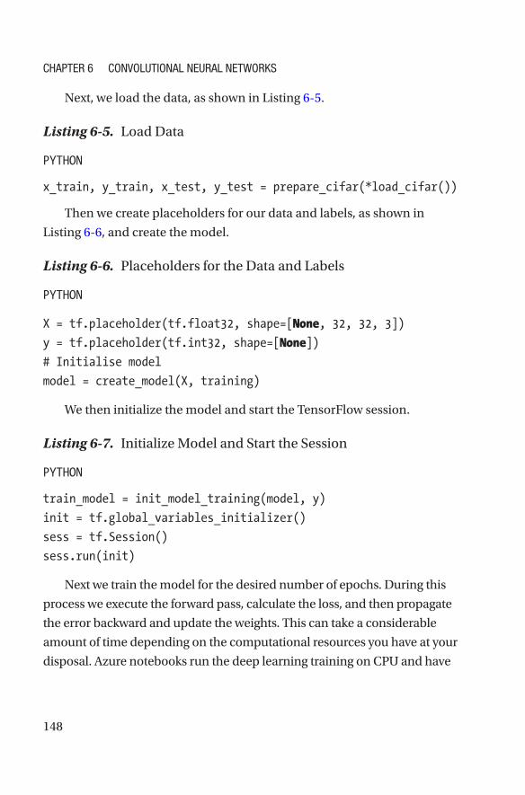
148
Next, we load the data, as shown in Listing 6-5.
Listing 6-5. Load Data
PYTHON
x_train, y_train, x_test, y_test = prepare_cifar(*load_cifar())
Then we create placeholders for our data and labels, as shown in
Listing 6-6, and create the model.
Listing 6-6. Placeholders for the Data and Labels
PYTHON
X = tf.placeholder(tf.float32, shape=[None, 32, 32, 3])
y = tf.placeholder(tf.int32, shape=[None])
# Initialise model
model = create_model(X, training)
We then initialize the model and start the TensorFlow session.
Listing 6-7. Initialize Model and Start the Session
PYTHON
train_model = init_model_training(model, y)
init = tf.global_variables_initializer()
sess = tf.Session()
sess.run(init)
Next we train the model for the desired number of epochs. During this
process we execute the forward pass, calculate the loss, and then propagate
the error backward and update the weights. This can take a considerable
amount of time depending on the computational resources you have at your
disposal. Azure notebooks run the deep learning training on CPU and have
Chapter 6 Convolutional neural networks
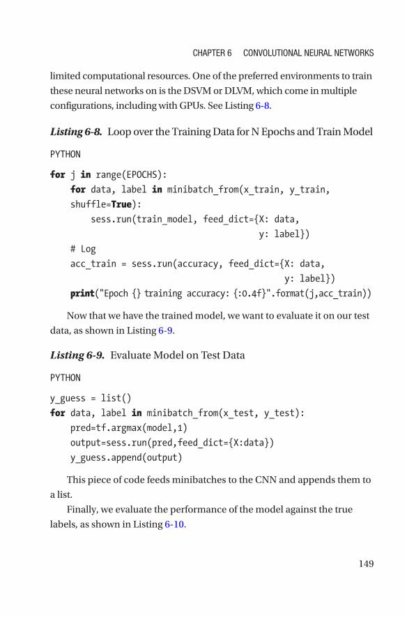
149
limited computational resources. One of the preferred environments to train
these neural networks on is the DSVM or DLVM, which come in multiple
configurations, including with GPUs. See Listing 6-8.
Listing 6-8. Loop over the Training Data for N Epochs and Train Model
PYTHON
for j in range(EPOCHS):
for data, label in minibatch_from(x_train, y_train,
shuffle=True):
sess.run(train_model, feed_dict={X: data,
y: label})
# Log
acc_train = sess.run(accuracy, feed_dict={X: data,
y: label})
print("Epoch {} training accuracy: {:0.4f}".format(j,acc_train))
Now that we have the trained model, we want to evaluate it on our test
data, as shown in Listing 6-9.
Listing 6-9. Evaluate Model on Test Data
PYTHON
y_guess = list()
for data, label in minibatch_from(x_test, y_test):
pred=tf.argmax(model,1)
output=sess.run(pred,feed_dict={X:data})
y_guess.append(output)
This piece of code feeds minibatches to the CNN and appends them to
a list.
Finally, we evaluate the performance of the model against the true
labels, as shown in Listing 6-10.
Chapter 6 Convolutional neural networks
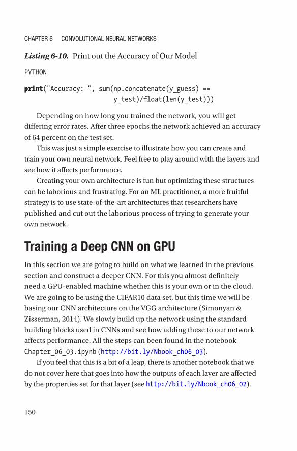
150
Listing 6-10. Print out the Accuracy of Our Model
PYTHON
print("Accuracy: ", sum(np.concatenate(y_guess) ==
y_test)/float(len(y_test)))
Depending on how long you trained the network, you will get
differing error rates. After three epochs the network achieved an accuracy
of 64 percent on the test set.
This was just a simple exercise to illustrate how you can create and
train your own neural network. Feel free to play around with the layers and
see how it affects performance.
Creating your own architecture is fun but optimizing these structures
can be laborious and frustrating. For an ML practitioner, a more fruitful
strategy is to use state-of-the-art architectures that researchers have
published and cut out the laborious process of trying to generate your
own network.
Training a Deep CNN on GPUIn this section we are going to build on what we learned in the previous
section and construct a deeper CNN. For this you almost definitely
need a GPU-enabled machine whether this is your own or in the cloud.
We are going to be using the CIFAR10 data set, but this time we will be
basing our CNN architecture on the VGG architecture (Simonyan &
Zisserman, 2014). We slowly build up the network using the standard
building blocks used in CNNs and see how adding these to our network
affects performance. All the steps can been found in the notebook
Chapter_06_03.ipynb (http://bit.ly/Nbook_ch06_03).
If you feel that this is a bit of a leap, there is another notebook that we
do not cover here that goes into how the outputs of each layer are affected
by the properties set for that layer (see http://bit.ly/Nbook_ch06_02).
Chapter 6 Convolutional neural networks
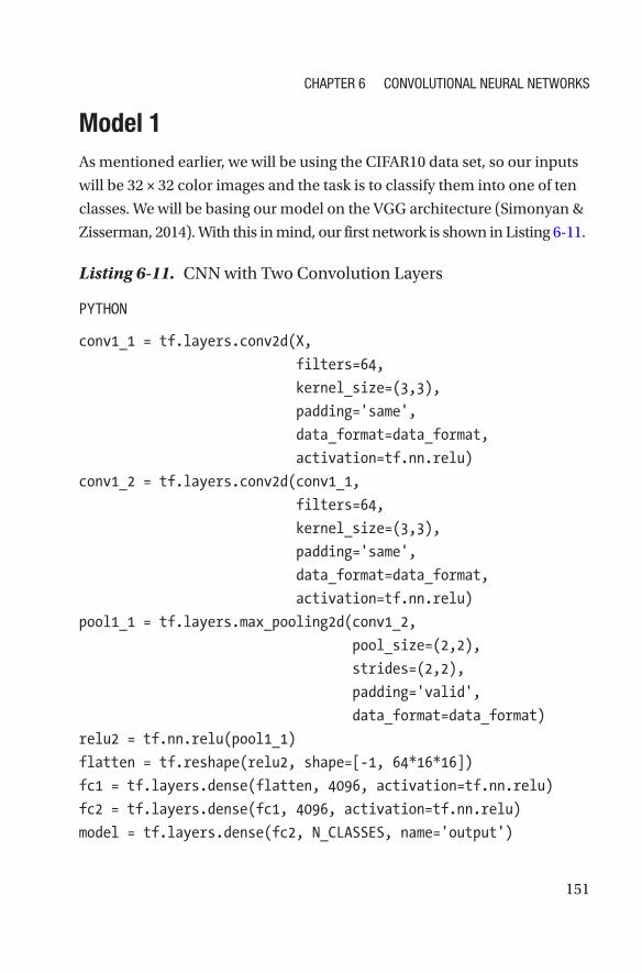
151
Model 1As mentioned earlier, we will be using the CIFAR10 data set, so our inputs
will be 32 × 32 color images and the task is to classify them into one of ten
classes. We will be basing our model on the VGG architecture (Simonyan &
Zisserman, 2014). With this in mind, our first network is shown in Listing 6-11.
Listing 6-11. CNN with Two Convolution Layers
PYTHON
conv1_1 = tf.layers.conv2d(X,
filters=64,
kernel_size=(3,3),
padding='same',
data_format=data_format,
activation=tf.nn.relu)
conv1_2 = tf.layers.conv2d(conv1_1,
filters=64,
kernel_size=(3,3),
padding='same',
data_format=data_format,
activation=tf.nn.relu)
pool1_1 = tf.layers.max_pooling2d(conv1_2,
pool_size=(2,2),
strides=(2,2),
padding='valid',
data_format=data_format)
relu2 = tf.nn.relu(pool1_1)
flatten = tf.reshape(relu2, shape=[-1, 64*16*16])
fc1 = tf.layers.dense(flatten, 4096, activation=tf.nn.relu)
fc2 = tf.layers.dense(fc1, 4096, activation=tf.nn.relu)
model = tf.layers.dense(fc2, N_CLASSES, name='output')
Chapter 6 Convolutional neural networks
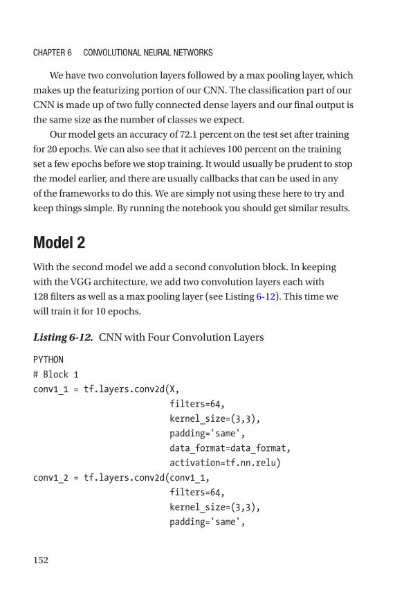
152
We have two convolution layers followed by a max pooling layer, which
makes up the featurizing portion of our CNN. The classification part of our
CNN is made up of two fully connected dense layers and our final output is
the same size as the number of classes we expect.
Our model gets an accuracy of 72.1 percent on the test set after training
for 20 epochs. We can also see that it achieves 100 percent on the training
set a few epochs before we stop training. It would usually be prudent to stop
the model earlier, and there are usually callbacks that can be used in any
of the frameworks to do this. We are simply not using these here to try and
keep things simple. By running the notebook you should get similar results.
Model 2With the second model we add a second convolution block. In keeping
with the VGG architecture, we add two convolution layers each with
128 filters as well as a max pooling layer (see Listing 6-12). This time we
will train it for 10 epochs.
Listing 6-12. CNN with Four Convolution Layers
PYTHON
# Block 1
conv1_1 = tf.layers.conv2d(X,
filters=64,
kernel_size=(3,3),
padding='same',
data_format=data_format,
activation=tf.nn.relu)
conv1_2 = tf.layers.conv2d(conv1_1,
filters=64,
kernel_size=(3,3),
padding='same',
Chapter 6 Convolutional neural networks
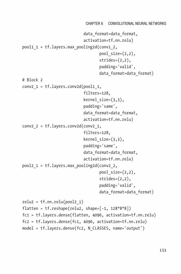
153
data_format=data_format,
activation=tf.nn.relu)
pool1_1 = tf.layers.max_pooling2d(conv1_2,
pool_size=(2,2),
strides=(2,2),
padding='valid',
data_format=data_format)
# Block 2
conv2_1 = tf.layers.conv2d(pool1_1,
filters=128,
kernel_size=(3,3),
padding='same',
data_format=data_format,
activation=tf.nn.relu)
conv2_2 = tf.layers.conv2d(conv2_1,
filters=128,
kernel_size=(3,3),
padding='same',
data_format=data_format,
activation=tf.nn.relu)
pool2_1 = tf.layers.max_pooling2d(conv2_2,
pool_size=(2,2),
strides=(2,2),
padding='valid',
data_format=data_format)
relu2 = tf.nn.relu(pool2_1)
flatten = tf.reshape(relu2, shape=[-1, 128*8*8])
fc1 = tf.layers.dense(flatten, 4096, activation=tf.nn.relu)
fc2 = tf.layers.dense(fc1, 4096, activation=tf.nn.relu)
model = tf.layers.dense(fc2, N_CLASSES, name='output')
Chapter 6 Convolutional neural networks

154
After training it for 10 epochs you should find the performance of your
model has improved slightly.
Model 3Let’s add another convolution block. This time, though, we increase the
number of filters to 256, again in keeping with the VGG architecture.
See Listing 6-13.
Listing 6-13. CNN with Seven Convolution Layers
PYTHON
# Block 1
conv1_1 = tf.layers.conv2d(X,
filters=64,
kernel_size=(3,3),
padding='same',
data_format=data_format,
activation=tf.nn.relu)
conv1_2 = tf.layers.conv2d(conv1_1,
filters=64,
kernel_size=(3,3),
padding='same',
data_format=data_format,
activation=tf.nn.relu)
pool1_1 = tf.layers.max_pooling2d(conv1_2,
pool_size=(2,2),
strides=(2,2),
padding='valid',
data_format=data_format)
Chapter 6 Convolutional neural networks

155
# Block 2
conv2_1 = tf.layers.conv2d(pool1_1,
filters=128,
kernel_size=(3,3),
padding='same',
data_format=data_format,
activation=tf.nn.relu)
conv2_2 = tf.layers.conv2d(conv2_1,
filters=128,
kernel_size=(3,3),
padding='same',
data_format=data_format,
activation=tf.nn.relu)
pool2_1 = tf.layers.max_pooling2d(conv2_2,
pool_size=(2,2),
strides=(2,2),
padding='valid',
data_format=data_format)
# Block 3
conv3_1 = tf.layers.conv2d(pool2_1,
filters=256,
kernel_size=(3,3),
padding='same',
data_format=data_format,
activation=tf.nn.relu)
conv3_2 = tf.layers.conv2d(conv3_1,
filters=256,
kernel_size=(3,3),
padding='same',
data_format=data_format,
activation=tf.nn.relu)
Chapter 6 Convolutional neural networks
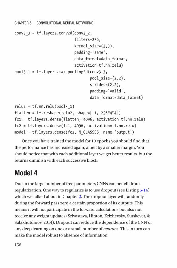
156
conv3_3 = tf.layers.conv2d(conv3_2,
filters=256,
kernel_size=(3,3),
padding='same',
data_format=data_format,
activation=tf.nn.relu)
pool3_1 = tf.layers.max_pooling2d(conv3_3,
pool_size=(2,2),
strides=(2,2),
padding='valid',
data_format=data_format)
relu2 = tf.nn.relu(pool3_1)
flatten = tf.reshape(relu2, shape=[-1, 256*4*4])
fc1 = tf.layers.dense(flatten, 4096, activation=tf.nn.relu)
fc2 = tf.layers.dense(fc1, 4096, activation=tf.nn.relu)
model = tf.layers.dense(fc2, N_CLASSES, name='output')
Once you have trained the model for 10 epochs you should find that
the performance has increased again, albeit by a smaller margin. You
should notice that with each additional layer we get better results, but the
returns diminish with each successive block.
Model 4Due to the large number of free parameters CNNs can benefit from
regularization. One way to regularize is to use dropout (see Listing 6-14),
which we talked about in Chapter 2. The dropout layer will randomly
during the forward pass zero a certain proportion of its outputs. This
means it will not participate in the forward calculations but also not
receive any weight updates (Srivastava, Hinton, Krizhevsky, Sutskever, &
Salakhutdinov, 2014). Dropout can reduce the dependence of the CNN or
any deep learning on one or a small number of neurons. This in turn can
make the model robust to absence of information.
Chapter 6 Convolutional neural networks
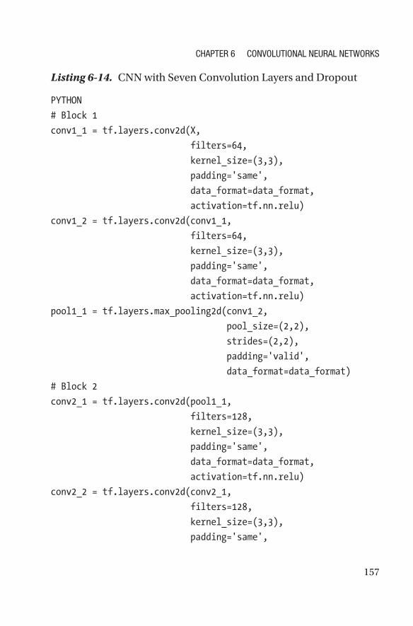
157
Listing 6-14. CNN with Seven Convolution Layers and Dropout
PYTHON
# Block 1
conv1_1 = tf.layers.conv2d(X,
filters=64,
kernel_size=(3,3),
padding='same',
data_format=data_format,
activation=tf.nn.relu)
conv1_2 = tf.layers.conv2d(conv1_1,
filters=64,
kernel_size=(3,3),
padding='same',
data_format=data_format,
activation=tf.nn.relu)
pool1_1 = tf.layers.max_pooling2d(conv1_2,
pool_size=(2,2),
strides=(2,2),
padding='valid',
data_format=data_format)
# Block 2
conv2_1 = tf.layers.conv2d(pool1_1,
filters=128,
kernel_size=(3,3),
padding='same',
data_format=data_format,
activation=tf.nn.relu)
conv2_2 = tf.layers.conv2d(conv2_1,
filters=128,
kernel_size=(3,3),
padding='same',
Chapter 6 Convolutional neural networks
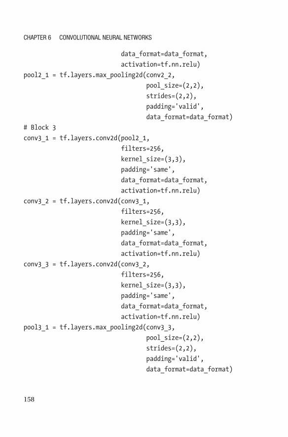
158
data_format=data_format,
activation=tf.nn.relu)
pool2_1 = tf.layers.max_pooling2d(conv2_2,
pool_size=(2,2),
strides=(2,2),
padding='valid',
data_format=data_format)
# Block 3
conv3_1 = tf.layers.conv2d(pool2_1,
filters=256,
kernel_size=(3,3),
padding='same',
data_format=data_format,
activation=tf.nn.relu)
conv3_2 = tf.layers.conv2d(conv3_1,
filters=256,
kernel_size=(3,3),
padding='same',
data_format=data_format,
activation=tf.nn.relu)
conv3_3 = tf.layers.conv2d(conv3_2,
filters=256,
kernel_size=(3,3),
padding='same',
data_format=data_format,
activation=tf.nn.relu)
pool3_1 = tf.layers.max_pooling2d(conv3_3,
pool_size=(2,2),
strides=(2,2),
padding='valid',
data_format=data_format)
Chapter 6 Convolutional neural networks
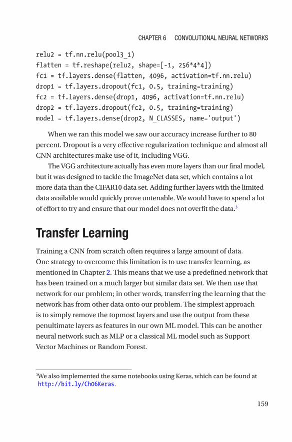
159
relu2 = tf.nn.relu(pool3_1)
flatten = tf.reshape(relu2, shape=[-1, 256*4*4])
fc1 = tf.layers.dense(flatten, 4096, activation=tf.nn.relu)
drop1 = tf.layers.dropout(fc1, 0.5, training=training)
fc2 = tf.layers.dense(drop1, 4096, activation=tf.nn.relu)
drop2 = tf.layers.dropout(fc2, 0.5, training=training)
model = tf.layers.dense(drop2, N_CLASSES, name='output')
When we ran this model we saw our accuracy increase further to 80
percent. Dropout is a very effective regularization technique and almost all
CNN architectures make use of it, including VGG.
The VGG architecture actually has even more layers than our final model,
but it was designed to tackle the ImageNet data set, which contains a lot
more data than the CIFAR10 data set. Adding further layers with the limited
data available would quickly prove untenable. We would have to spend a lot
of effort to try and ensure that our model does not overfit the data.3
Transfer LearningTraining a CNN from scratch often requires a large amount of data.
One strategy to overcome this limitation is to use transfer learning, as
mentioned in Chapter 2. This means that we use a predefined network that
has been trained on a much larger but similar data set. We then use that
network for our problem; in other words, transferring the learning that the
network has from other data onto our problem. The simplest approach
is to simply remove the topmost layers and use the output from these
penultimate layers as features in our own ML model. This can be another
neural network such as MLP or a classical ML model such as Support
Vector Machines or Random Forest.
3 We also implemented the same notebooks using Keras, which can be found at http://bit.ly/Ch06Keras.
Chapter 6 Convolutional neural networks
160
Another approach is to replace the topmost fully connected layers and
then freeze certain layers and retrain it. Freezing layers means that the
weights of these layers are not updated during training. Which layers to
freeze depends on a number of factors, including the similarity between
the data sets used and so on. Retraining more layers can often improve the
accuracy of the model, but also increases the possibility of overfitting.
Almost all network topologies published have pretrained weights for
the ImageNet data set, one of the largest image classification data sets and
more or less the standard for image classification problems. This data set
consists of millions of images spanning multiple classes (ImageNet, n.d.).
Using pretrained CNNs trained on ImageNet is an easy way to get very
good results for image classification tasks.
SummaryThis chapter briefly described what constitutes a CNN. We have explained
why convolution is useful in computer vision tasks, as well as what the
shortcomings of CNNs are. We went through a simple example of creating
a CNN in TensorFlow and then expanded on it through a series of steps
and observed the effect it had on the performance of the model. This
chapter has only scratched the surface of the vast information on CNNs,
with many great books covering the theory behind them. The next chapter
goes over a different deep learning architecture, RNNs, which are well
suited to the tasks of sequence modeling such as language translation.
Chapter 6 Convolutional neural networks

161© Mathew Salvaris, Danielle Dean, Wee Hyong Tok 2018 M. Salvaris et al., Deep Learning with Azure, https://doi.org/10.1007/978-1-4842-3679-6_7
CHAPTER 7
Recurrent Neural NetworksThe previous chapter showed how a deep learning model—specifically
CNNs—could be applied to images. The process could be decoupled into
a feature extractor that figures out the optimal hidden-state representation
of the input (in this case a vector of feature maps) and a classifier
(typically a fully connected layer). This chapter focuses on the hidden-
state representation of other forms of data and explores RNNs. RNNs are
especially useful for analyzing sequences, which is particularly helpful for
natural language processing and time series analysis.
Even images can be thought of as a subset of sequence data; if we
shuffle the rows and columns (or channels) then the image becomes
unrecognizable. This is not the case for spreadsheet data, for example.
However, CNNs have a very weak notion of order and typically the kernel
size for a convolution is in the single digits. As these convolutions are
stacked on top of each other, the receptive field increases, but the signal
also gets dampened. This means that CNNs typically only care about
temporary spatial relationships, such as a nose or eye. In Figure 7-1, we
can imagine that we have shuffled a sequence, preserving order only
within local groups, but most CNNs will still classify it the same, even
though it makes no sense overall.
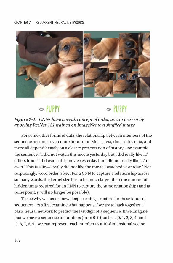
162
For some other forms of data, the relationship between members of the
sequence becomes even more important. Music, text, time series data, and
more all depend heavily on a clear representation of history. For example
the sentence, “I did not watch this movie yesterday but I did really like it,”
differs from “I did watch this movie yesterday but I did not really like it,” or
even “This is a lie—I really did not like the movie I watched yesterday.” Not
surprisingly, word order is key. For a CNN to capture a relationship across
so many words, the kernel size has to be much larger than the number of
hidden units required for an RNN to capture the same relationship (and at
some point, it will no longer be possible).
To see why we need a new deep learning structure for these kinds of
sequences, let’s first examine what happens if we try to hack together a
basic neural network to predict the last digit of a sequence. If we imagine
that we have a sequence of numbers (from 0–9) such as [0, 1, 2, 3, 4] and
[9, 8, 7, 6, 5], we can represent each number as a 10-dimensional vector
Figure 7-1. CNNs have a weak concept of order, as can be seen by applying ResNet-121 trained on ImageNet to a shuffled image
Chapter 7 reCurrent neural networks

163
that is one-hot encoded. For example, the number 2 could be encoded as
[0, 0, 1, 0, 0, 0, 0, 0, 0, 0] and 6 as [0, 0, 0, 0, 0, 0, 1, 0, 0, 0]. To train a network
to predict the last digit of the sequence we can attempt two different
approaches.
First, we can concatenate the four one-hot encoded vectors and thus
create a hidden state that exists in 40-dimensional space. The neural
network then adjusts a weights matrix (size 40 × 10) and a bias matrix
(size 10 × 1) to map this to the label (the last number), which exists in a
10-dimensional space. Second, we can sum the input vectors together
and create a hidden state that exists in 10-dimensional space and train the
network to map this to the label instead.
The issue with the second approach is that by summing the one-hot
encoded vector for 2 and 3, for example, we get [0, 0, 1, 1, 0, 0, 0, 0, 0, 0]
and with this hidden state it is not possible to know whether the input
sequence was [2, 3] or [3, 2] and thus whether the next number should be 4
or 1. The first approach does not have this issue because we can clearly see
that [0, 0, 1, 0, 0, 0, 0, 0, 0, 0, 0, 0, 0, 1, 0, 0, 0, 0, 0, 0] corresponds to [2, 3].
However, another issue arises when we see that we have learned a weights
matrix that is of size (40 × 10). Our neural network can only work with an
input of four numbers.
Hence, by summing inputs we can work with variable-length
sequences, but we cannot preserve order. In contrast, by concatenating
inputs we can preserve order, but we have to work with a sequence of a
fixed size. RNNs solve this by representing history as a fixed-dimension
vector that handles inputs that are variable-length sequences (and as
we will see in the sequences-to-sequence section, also variable-length
outputs).
The operation of an RNN can be represented as the second neural
network in the preceding example: summing input vectors, but with the
modification that after every summation we multiply the hidden state
by some number. This number remains the same for all time steps and
thus RNNs make use of weight sharing, in a similar manner to CNNs.
Chapter 7 reCurrent neural networks
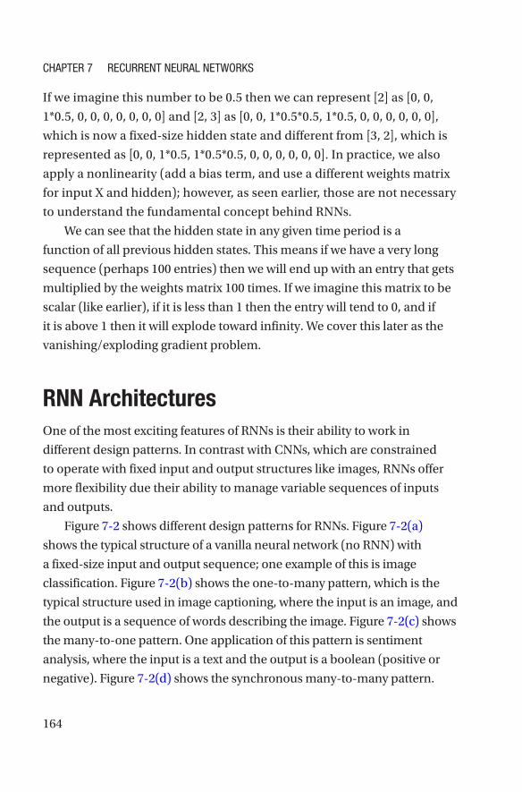
164
If we imagine this number to be 0.5 then we can represent [2] as [0, 0,
1*0.5, 0, 0, 0, 0, 0, 0, 0] and [2, 3] as [0, 0, 1*0.5*0.5, 1*0.5, 0, 0, 0, 0, 0, 0],
which is now a fixed-size hidden state and different from [3, 2], which is
represented as [0, 0, 1*0.5, 1*0.5*0.5, 0, 0, 0, 0, 0, 0]. In practice, we also
apply a nonlinearity (add a bias term, and use a different weights matrix
for input X and hidden); however, as seen earlier, those are not necessary
to understand the fundamental concept behind RNNs.
We can see that the hidden state in any given time period is a
function of all previous hidden states. This means if we have a very long
sequence (perhaps 100 entries) then we will end up with an entry that gets
multiplied by the weights matrix 100 times. If we imagine this matrix to be
scalar (like earlier), if it is less than 1 then the entry will tend to 0, and if
it is above 1 then it will explode toward infinity. We cover this later as the
vanishing/exploding gradient problem.
RNN ArchitecturesOne of the most exciting features of RNNs is their ability to work in
different design patterns. In contrast with CNNs, which are constrained
to operate with fixed input and output structures like images, RNNs offer
more flexibility due their ability to manage variable sequences of inputs
and outputs.
Figure 7-2 shows different design patterns for RNNs. Figure 7-2(a)
shows the typical structure of a vanilla neural network (no RNN) with
a fixed-size input and output sequence; one example of this is image
classification. Figure 7-2(b) shows the one-to-many pattern, which is the
typical structure used in image captioning, where the input is an image, and
the output is a sequence of words describing the image. Figure 7- 2(c) shows
the many-to-one pattern. One application of this pattern is sentiment
analysis, where the input is a text and the output is a boolean (positive or
negative). Figure 7-2(d) shows the synchronous many-to- many pattern.
Chapter 7 reCurrent neural networks

165
An example of this could be video captioning, where we want to set a tag
to each video frame. Finally, Figure 7-2(e) shows the asynchronous many-
to-many representation, which is the typical case of machine translation,
where the input could be text in English and the output text in Spanish.
Figure 7-2. Bottom layer is the inputs, in the middle are the hidden states, and the top layer is the outputs. (a) Vanilla network (no RNN) with single input, hidden state, and single output. (b) One-to-many pattern. (c) Many-to-one pattern. (d) Synchronous many-to-many pattern. (e) Asynchronous many-to-many pattern, also referred as encoder–decoder.
Apart from the previous design patterns, RNNs vary depending on
how the interconnection between the different layers is performed. The
standard case is where the RNN has recurrent connections between
hidden units, as depicted in Figure 7-3. In this case, the RNN is Turing-
complete (Siegelmann, 1995), and therefore can simulate any arbitrary
program. In essence, an RNN repeatedly applies a nonlinear function,
with trainable parameters to a hidden state, which make them suitable for
sequence modeling tasks.
Chapter 7 reCurrent neural networks
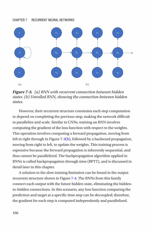
166
However, their recurrent structure constrains each step computation
to depend on completing the previous step, making the network difficult
to parallelize and scale. Similar to CNNs, training an RNN involves
computing the gradient of the loss function with respect to the weights.
This operation involves computing a forward propagation, moving from
left to right through in Figure 7-3(b), followed by a backward propagation,
moving from right to left, to update the weights. This training process is
expensive because the forward propagation is inherently sequential, and
thus cannot be parallelized. The backpropagation algorithm applied in
RNNs is called backpropagation through time (BPTT), and is discussed in
detail later in this chapter.
A solution to the slow training limitation can be found in the output
recurrent structure shown in Figure 7-4. The RNNs from this family
connect each output with the future hidden state, eliminating the hidden-
to- hidden connections. In this scenario, any loss function comparing the
prediction and target at a specific time step can be decoupled; therefore,
the gradient for each step is computed independently and parallelized.
Figure 7-3. (a) RNN with recurrent connection between hidden states. (b) Unrolled RNN, showing the connection between hidden states.
Chapter 7 reCurrent neural networks
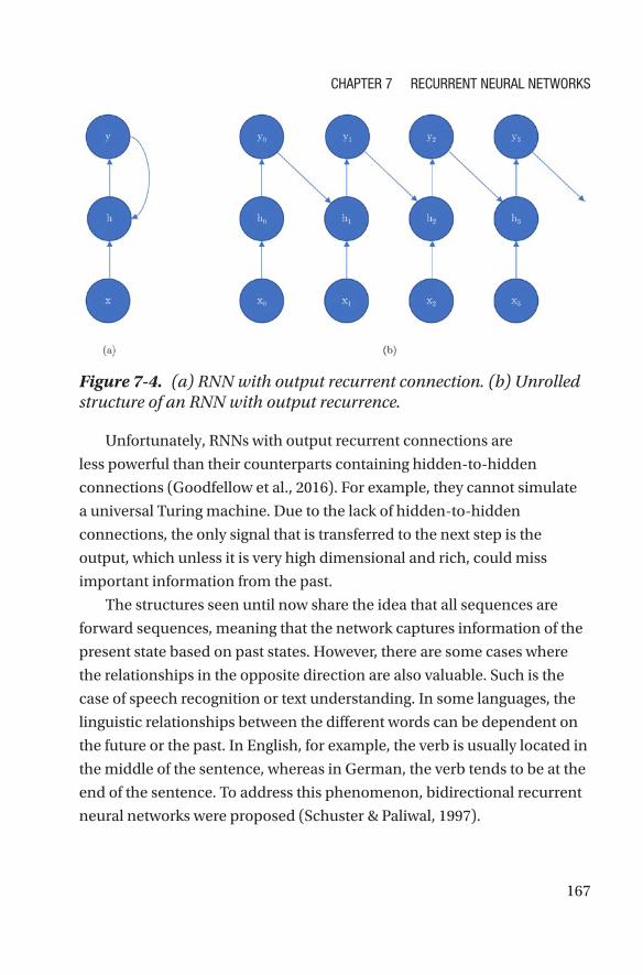
167
Unfortunately, RNNs with output recurrent connections are
less powerful than their counterparts containing hidden-to-hidden
connections (Goodfellow et al., 2016). For example, they cannot simulate
a universal Turing machine. Due to the lack of hidden-to-hidden
connections, the only signal that is transferred to the next step is the
output, which unless it is very high dimensional and rich, could miss
important information from the past.
The structures seen until now share the idea that all sequences are
forward sequences, meaning that the network captures information of the
present state based on past states. However, there are some cases where
the relationships in the opposite direction are also valuable. Such is the
case of speech recognition or text understanding. In some languages, the
linguistic relationships between the different words can be dependent on
the future or the past. In English, for example, the verb is usually located in
the middle of the sentence, whereas in German, the verb tends to be at the
end of the sentence. To address this phenomenon, bidirectional recurrent
neural networks were proposed (Schuster & Paliwal, 1997).
Figure 7-4. (a) RNN with output recurrent connection. (b) Unrolled structure of an RNN with output recurrence.
Chapter 7 reCurrent neural networks
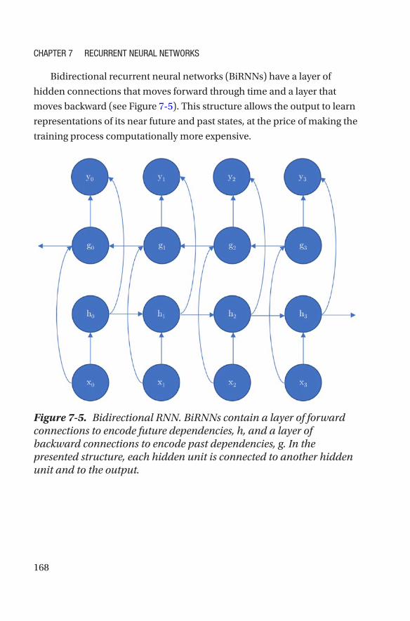
168
Bidirectional recurrent neural networks (BiRNNs) have a layer of
hidden connections that moves forward through time and a layer that
moves backward (see Figure 7-5). This structure allows the output to learn
representations of its near future and past states, at the price of making the
training process computationally more expensive.
Figure 7-5. Bidirectional RNN. BiRNNs contain a layer of forward connections to encode future dependencies, h, and a layer of backward connections to encode past dependencies, g. In the presented structure, each hidden unit is connected to another hidden unit and to the output.
Chapter 7 reCurrent neural networks
169
Training RNNsRNN training shares some similarities with the CNN training method that
we saw in the previous chapter, but in the RNN case, the algorithm used is
called BPTT (Werbos, 1990). The underlying idea behind BPTT is simply
to apply the same generalized backpropagation algorithm to the unrolled
computational graph. The steps of training an RNN are as follows:
1. We have an RNN architecture like the ones shown in
Figure 7-3, Figure 7-4, and Figure 7-5. The weights
are initialized based on some distribution.
2. We input the sequences as minibatches to the RNN
as (batch size, sequence size). The sequence size can
have a variable length depending on the framework
you are using.
3. We compute the forward propagation by unrolling
the graph and obtaining the predicted output at
each time step.
4. We compare the predicted output with the true
labels and accumulate the error (or loss) across each
time step.
5. We apply backpropagation by computing the
gradient of the loss with respect to the weights and
use gradient descent to update the weights.
6. This process is repeated for a number of epochs or
until some exit criteria are met.
For long sequences, there is a high cost of updating the weights.
For instance, the gradient of an RNN with sequences of length 1,000 is
equivalent to a forward and a backward pass in a neural network with
1,000 layers (Sutskever, 2013).
Chapter 7 reCurrent neural networks

170
Therefore, a practical approach for training RNNs is to compute
BPTT in a sliding window of the unrolled graph, which is referred as
truncated BPTT (Williams & Peng, 1990). The idea is simple: Each
complete sequence is sliced into a number of smaller subsequences
and BPTT is applied to each of these parts. This approach works well in
practice, especially in word modeling problems (Mikolov, Karafiát, Burget,
Černocký, & Khudanpur, 2010), but the algorithm is blind to dependencies
between different windows.
Gated RNNsDue to the iterative nature of the propagation error in RNNs, in some cases,
the loss gradients can vanish as they get backpropagated in time. This
is referred to as vanishing gradients (Bengio, Simard, & Frasconi, 1994).
A vanishing gradient means in practice that the loss gradient is a small
quantity, therefore the process of updating the weights can take too long.
More rarely, the gradient can explode, producing gradients exponentially
large, referred to as exploding gradients. This also makes RNNs difficult to
train on sequences with long temporal dependencies.
A solution to the vanishing and exploding gradient problem is
the LSTM RNN (Gers, Schmidhuber, & Cummins, 2000; Hochreiter &
Schmidhuber, 1997), which is a network type specially designed to learn
long-term relationships. For it, they substitute the hidden units of standard
RNNs with a new block called the LSTM cell. The intuition behind these
cells is that they allow control of the amount of information that is going
to be passed to the next state and use a forgetting mechanism to stop the
information that is not useful anymore.
The LSTM block (see Figure 7-6) is composed of a state unit and three
gating units: forget gate, input gate, and output gate. At a high level, the
state unit handles the information transfer between the input and the
output, and contains a self-loop. The gating units, which simply set their
Chapter 7 reCurrent neural networks
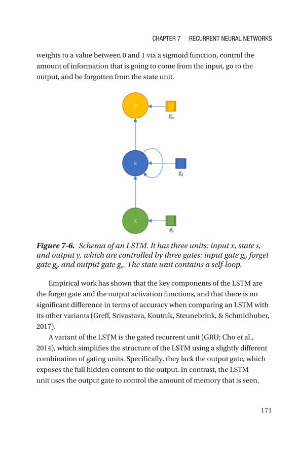
171
weights to a value between 0 and 1 via a sigmoid function, control the
amount of information that is going to come from the input, go to the
output, and be forgotten from the state unit.
Figure 7-6. Schema of an LSTM. It has three units: input x, state s, and output y, which are controlled by three gates: input gate gi, forget gate gf, and output gate go. The state unit contains a self-loop.
Empirical work has shown that the key components of the LSTM are
the forget gate and the output activation functions, and that there is no
significant difference in terms of accuracy when comparing an LSTM with
its other variants (Greff, Srivastava, Koutník, Steunebrink, & Schmidhuber,
2017).
A variant of the LSTM is the gated recurrent unit (GRU; Cho et al.,
2014), which simplifies the structure of the LSTM using a slightly different
combination of gating units. Specifically, they lack the output gate, which
exposes the full hidden content to the output. In contrast, the LSTM
unit uses the output gate to control the amount of memory that is seen.
Chapter 7 reCurrent neural networks

172
This lack of the output gate in GRUs makes them computationally less
expensive, but it could lead to a suboptimal memory representation, which
might be the reason an LSTM tends to remember longer sequences. For
a more detailed comparison between LSTMs and GRUs, please refer to
Chung, Gulcehre, Cho, & Bengio, 2014).
Sequence-to-Sequence Models and Attention MechanismSequence-to-sequence models (Cho et al., 2014; Sutskever, Vinyals, &
Le, 2014) are a relatively recent architecture that have created many
exciting possibilities for machine translation, speech recognition, and text
summarization. The basic principle is to map an input sequence to an
output sequence, which can be of a different length, a variant of Figure 7- 2(e)
This is accomplished by combining an input RNN (or an encoder) that maps
a variable-length sequence to a fixed-length vector with an output RNN (or
a decoder) that maps a fixed-length vector to a variable- length sequence. As
an example, see the blog post with associated tutorial for generating music
using an LSTM sequence-to-sequence model with Azure Machine Learning
from Erika Menezes available at http://bit.ly/MusicGenAzure.
Sequence-to-sequence models in the realm of machine translation
(called neural machine translation [NMT]) have largely replaced phrase-
based machine translation because they do not require lots of manual
tuning for each subcomponent (and for each language). NMT (shown in
Figure 7-7) models might have different RNN structures for the encoder
and the decoder component; the structure of the RNNs can vary in several
ways: cell type such as GRU or LSTM, number of layers, and directionality
(unidirectional or bidirectional).
Chapter 7 reCurrent neural networks
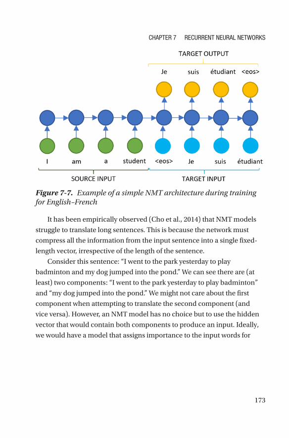
173
It has been empirically observed (Cho et al., 2014) that NMT models
struggle to translate long sentences. This is because the network must
compress all the information from the input sentence into a single fixed-
length vector, irrespective of the length of the sentence.
Consider this sentence: “I went to the park yesterday to play
badminton and my dog jumped into the pond.” We can see there are (at
least) two components: “I went to the park yesterday to play badminton”
and “my dog jumped into the pond.” We might not care about the first
component when attempting to translate the second component (and
vice versa). However, an NMT model has no choice but to use the hidden
vector that would contain both components to produce an input. Ideally,
we would have a model that assigns importance to the input words for
Figure 7-7. Example of a simple NMT architecture during training for English–French
Chapter 7 reCurrent neural networks
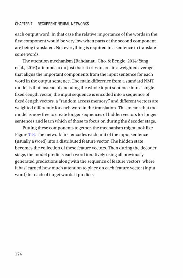
174
each output word. In that case the relative importance of the words in the
first component would be very low when parts of the second component
are being translated. Not everything is required in a sentence to translate
some words.
The attention mechanism (Bahdanau, Cho, & Bengio, 2014; Yang
et al., 2016) attempts to do just that: It tries to create a weighted average
that aligns the important components from the input sentence for each
word in the output sentence. The main difference from a standard NMT
model is that instead of encoding the whole input sentence into a single
fixed-length vector, the input sequence is encoded into a sequence of
fixed-length vectors, a “random access memory,” and different vectors are
weighted differently for each word in the translation. This means that the
model is now free to create longer sequences of hidden vectors for longer
sentences and learn which of those to focus on during the decoder stage.
Putting these components together, the mechanism might look like
Figure 7-8. The network first encodes each unit of the input sentence
(usually a word) into a distributed feature vector. The hidden state
becomes the collection of these feature vectors. Then during the decoder
stage, the model predicts each word iteratively using all previously
generated predictions along with the sequence of feature vectors, where
it has learned how much attention to place on each feature vector (input
word) for each of target words it predicts.
Chapter 7 reCurrent neural networks
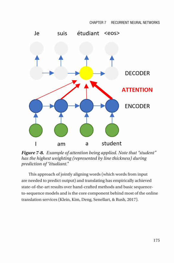
175
This approach of jointly aligning words (which words from input
are needed to predict output) and translating has empirically achieved
state-of-the-art results over hand-crafted methods and basic sequence-
to- sequence models and is the core component behind most of the online
translation services (Klein, Kim, Deng, Senellart, & Rush, 2017).
Figure 7-8. Example of attention being applied. Note that “student” has the highest weighting (represented by line thickness) during prediction of “étudiant.”
Chapter 7 reCurrent neural networks

176
RNN ExamplesIn this section, we are going to study two examples of RNNs implemented
in TensorFlow. The code is available at http://bit.ly/AzureRNNCode.
The first example runs sentiment analysis in TensorFlow as well as
several other frameworks. The second example builds off the example in
Chapter 6 to illustrate the differences between CNNs and RNNs on image
classification. The third example uses RNNs for time series analysis.
More Info we recommend provisioning an azure DlVM to run the code examples in this chapter. please see Chapter 4 for more information.
Example 1: Sentiment AnalysisWe first highly recommend the examples available at http://bit.ly/
DLComparisons, which at the time of this writing include six different
Python deep learning framework implementations for an RNN (GRU)
to predict sentiment on the IMDB movie review data set, as well as an
implementation in R (Keras with TensorFlow back end) as well as Julia
(Knet). These examples include training times for an NC series DLVM
(NVIDIA Tesla K80 GPU) as well as an NC_v2 series DLVM (NDIVIA Tesla
P100 GPU) so one can follow along and also compare timings to make sure
the setup is correct.
Example 2: Image ClassificationIn Chapter 6, we saw how a CNN is typically used to classify an image.
Here, we examine how to do the same but with an RNN. Although this is
not a traditional application of RNNs, it illustrates that it is often possible
Chapter 7 reCurrent neural networks
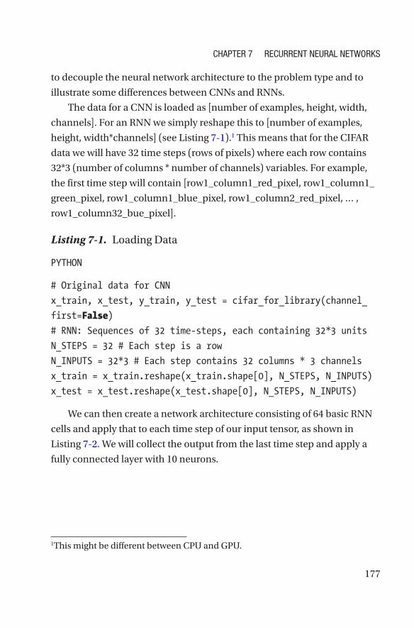
177
to decouple the neural network architecture to the problem type and to
illustrate some differences between CNNs and RNNs.
The data for a CNN is loaded as [number of examples, height, width,
channels]. For an RNN we simply reshape this to [number of examples,
height, width*channels] (see Listing 7-1).1 This means that for the CIFAR
data we will have 32 time steps (rows of pixels) where each row contains
32*3 (number of columns * number of channels) variables. For example,
the first time step will contain [row1_column1_red_pixel, row1_column1_
green_pixel, row1_column1_blue_pixel, row1_column2_red_pixel, … ,
row1_column32_bue_pixel].
Listing 7-1. Loading Data
PYTHON
# Original data for CNN
x_train, x_test, y_train, y_test = cifar_for_library(channel_
first=False)
# RNN: Sequences of 32 time-steps, each containing 32*3 units
N_STEPS = 32 # Each step is a row
N_INPUTS = 32*3 # Each step contains 32 columns * 3 channels
x_train = x_train.reshape(x_train.shape[0], N_STEPS, N_INPUTS)
x_test = x_test.reshape(x_test.shape[0], N_STEPS, N_INPUTS)
We can then create a network architecture consisting of 64 basic RNN
cells and apply that to each time step of our input tensor, as shown in
Listing 7-2. We will collect the output from the last time step and apply a
fully connected layer with 10 neurons.
1 This might be different between CPU and GPU.
Chapter 7 reCurrent neural networks
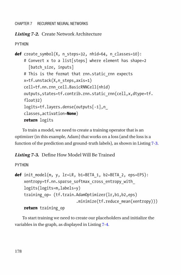
178
Listing 7-2. Create Network Architecture
PYTHON
def create_symbol(X, n_steps=32, nhid=64, n_classes=10):
# Convert x to a list[steps] where element has shape=2
[batch_size, inputs]
# This is the format that rnn.static_rnn expects
x=tf.unstack(X,n_steps,axis=1)
cell=tf.nn.rnn_cell.BasicRNNCell(nhid)
outputs,states=tf.contrib.rnn.static_rnn(cell,x,dtype=tf.
float32)
logits=tf.layers.dense(outputs[-1],n_
classes,activation=None)
return logits
To train a model, we need to create a training operator that is an
optimizer (in this example, Adam) that works on a loss (and the loss is a
function of the prediction and ground-truth labels), as shown in Listing 7-3.
Listing 7-3. Define How Model Will Be Trained
PYTHON
def init_model(m, y, lr=LR, b1=BETA_1, b2=BETA_2, eps=EPS):
xentropy=tf.nn.sparse_softmax_cross_entropy_with_
logits(logits=m,labels=y)
training_op= (tf.train.AdamOptimizer(lr,b1,b2,eps)
.minimize(tf.reduce_mean(xentropy)))
return training_op
To start training we need to create our placeholders and initialize the
variables in the graph, as displayed in Listing 7-4.
Chapter 7 reCurrent neural networks

179
Listing 7-4. Placeholders and Initialization
PYTHON
# Placeholders
X = tf.placeholder(tf.float32, shape=[None, N_STEPS, N_INPUTS])
y=tf.placeholder(tf.int32,shape=[None]) # Sparse
# Initialize model
sym = create_symbol(X)
model = init_model(sym, y)
sess = tf.Session()
sess.run(tf.global_variables_initializer())
We can then train our model as shown in Listing 7-5.
Listing 7-5. Training Model
PYTHON
for j in range(EPOCHS):
for data,label in yield_mb(x_train,y_train,BATCHSIZE,
shuffle=True):
sess.run(model,feed_dict={X:data,y:label})
The generator to supply our data is created as shown in Listing 7-6.
Listing 7-6. Generator to Supply Data to Model
PYTHON
def shuffle_data(X, y):
s=np.arange(len(X))
np.random.shuffle(s)
X=X[s]
y=y[s]
return X,y
Chapter 7 reCurrent neural networks
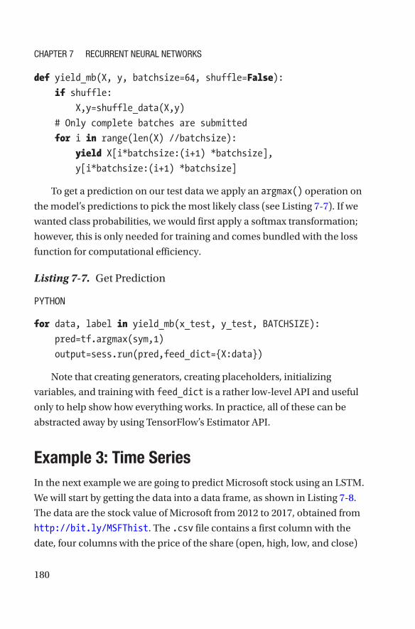
180
def yield_mb(X, y, batchsize=64, shuffle=False):
if shuffle:
X,y=shuffle_data(X,y)
# Only complete batches are submitted
for i in range(len(X) //batchsize):
yield X[i*batchsize:(i+1) *batchsize],
y[i*batchsize:(i+1) *batchsize]
To get a prediction on our test data we apply an argmax() operation on
the model’s predictions to pick the most likely class (see Listing 7-7). If we
wanted class probabilities, we would first apply a softmax transformation;
however, this is only needed for training and comes bundled with the loss
function for computational efficiency.
Listing 7-7. Get Prediction
PYTHON
for data, label in yield_mb(x_test, y_test, BATCHSIZE):
pred=tf.argmax(sym,1)
output=sess.run(pred,feed_dict={X:data})
Note that creating generators, creating placeholders, initializing
variables, and training with feed_dict is a rather low-level API and useful
only to help show how everything works. In practice, all of these can be
abstracted away by using TensorFlow’s Estimator API.
Example 3: Time SeriesIn the next example we are going to predict Microsoft stock using an LSTM.
We will start by getting the data into a data frame, as shown in Listing 7-8.
The data are the stock value of Microsoft from 2012 to 2017, obtained from
http://bit.ly/MSFThist. The .csv file contains a first column with the
date, four columns with the price of the share (open, high, low, and close)
Chapter 7 reCurrent neural networks
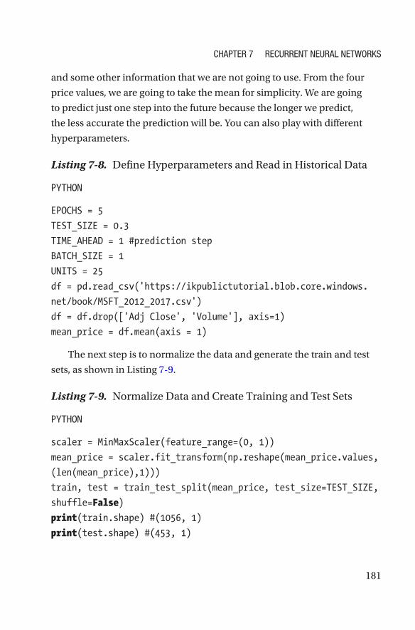
181
and some other information that we are not going to use. From the four
price values, we are going to take the mean for simplicity. We are going
to predict just one step into the future because the longer we predict,
the less accurate the prediction will be. You can also play with different
hyperparameters.
Listing 7-8. Define Hyperparameters and Read in Historical Data
PYTHON
EPOCHS = 5
TEST_SIZE = 0.3
TIME_AHEAD = 1 #prediction step
BATCH_SIZE = 1
UNITS = 25
df = pd.read_csv('https://ikpublictutorial.blob.core.windows.
net/book/MSFT_2012_2017.csv')
df = df.drop(['Adj Close', 'Volume'], axis=1)
mean_price = df.mean(axis = 1)
The next step is to normalize the data and generate the train and test
sets, as shown in Listing 7-9.
Listing 7-9. Normalize Data and Create Training and Test Sets
PYTHON
scaler = MinMaxScaler(feature_range=(0, 1))
mean_price = scaler.fit_transform(np.reshape(mean_price.values,
(len(mean_price),1)))
train, test = train_test_split(mean_price, test_size=TEST_SIZE,
shuffle=False)
print(train.shape) #(1056, 1)
print(test.shape) #(453, 1)
Chapter 7 reCurrent neural networks
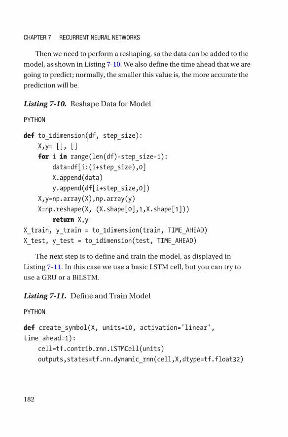
182
Then we need to perform a reshaping, so the data can be added to the
model, as shown in Listing 7-10. We also define the time ahead that we are
going to predict; normally, the smaller this value is, the more accurate the
prediction will be.
Listing 7-10. Reshape Data for Model
PYTHON
def to_1dimension(df, step_size):
X,y= [], []
for i in range(len(df)-step_size-1):
data=df[i:(i+step_size),0]
X.append(data)
y.append(df[i+step_size,0])
X,y=np.array(X),np.array(y)
X=np.reshape(X, (X.shape[0],1,X.shape[1]))
return X,y
X_train, y_train = to_1dimension(train, TIME_AHEAD)
X_test, y_test = to_1dimension(test, TIME_AHEAD)
The next step is to define and train the model, as displayed in
Listing 7-11. In this case we use a basic LSTM cell, but you can try to
use a GRU or a BiLSTM.
Listing 7-11. Define and Train Model
PYTHON
def create_symbol(X, units=10, activation='linear',
time_ahead=1):
cell=tf.contrib.rnn.LSTMCell(units)
outputs,states=tf.nn.dynamic_rnn(cell,X,dtype=tf.float32)
Chapter 7 reCurrent neural networks

183
sym=tf.layers.dense(outputs[-1],1,activation=None,name='out
put')
return sym
X = tf.placeholder(tf.float32, shape=[None, 1, TIME_AHEAD])
y = tf.placeholder(tf.float32, shape=[None])
sym = create_symbol(X, units=UNITS, time_ahead=TIME_AHEAD)
loss = tf.reduce_mean(tf.squared_difference(sym, y)) #mse
optimizer = tf.train.AdamOptimizer()
model = optimizer.minimize(loss)
init = tf.global_variables_initializer()
sess = tf.Session()
sess.run(init)
for i in range(EPOCHS):
ii=0
while(ii+BATCH_SIZE) <=len(X_train):
X_batch=X_train[ii:ii+BATCH_SIZE,:,:]
y_batch=y_train[ii:ii+BATCH_SIZE]
sess.run(model,feed_dict={X:X_batch,y:y_batch})
ii+=BATCH_SIZE
loss_train=sess.run(loss,feed_dict={X:X_batch,y:y_batch})
print('Epoch {}/{}'.format(i+1,EPOCHS),' Current loss: {}'.
format(loss_train))
Finally, we are going to calculate the root mean squared error (RMSE)
of the test set prediction, as shown in Listing 7-12.
Chapter 7 reCurrent neural networks

184
Listing 7-12. Calculate Test Set RMSE
PYTHON
y_guess = np.zeros(y_test.shape[0], dtype=np.float32)
ii = 0
while(ii + BATCH_SIZE) <= len(X_test):
X_batch=X_test[ii:ii+BATCH_SIZE,:,:]
output=sess.run(sym,feed_dict={X:X_batch})
y_guess[ii:ii+BATCH_SIZE] =output
ii+=BATCH_SIZE
y_test_inv = scaler.inverse_transform([y_test])
pred_test = scaler.inverse_transform([y_guess])
score = math.sqrt(mean_squared_error(y_test_inv, pred_test))
print('Test RMSE: %.2f' % (score)) #3.52
Looking at Figure 7-9, it seems that the LSTM is predicting the stocks
well. Now you can play with different time horizons or LSTM parameters.
This was a simple example of using LSTMs for time series analysis to
illustrate the concept of using LSTMs in forecasting.
Chapter 7 reCurrent neural networks
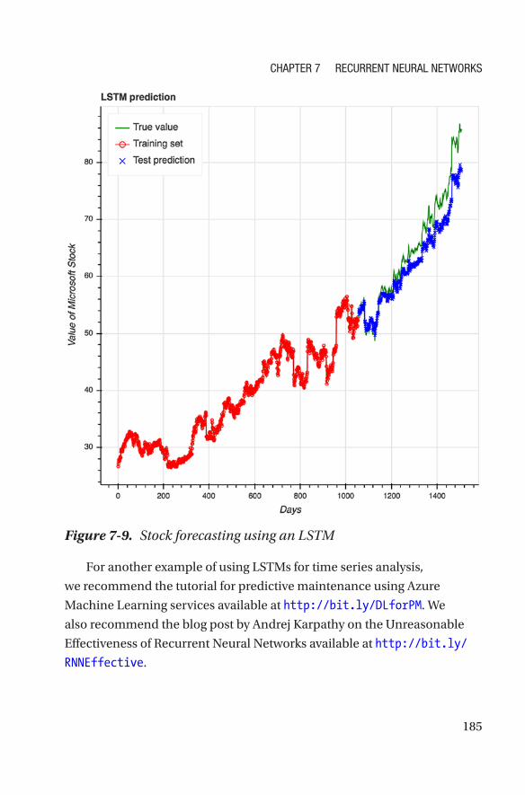
185
For another example of using LSTMs for time series analysis,
we recommend the tutorial for predictive maintenance using Azure
Machine Learning services available at http://bit.ly/DLforPM. We
also recommend the blog post by Andrej Karpathy on the Unreasonable
Effectiveness of Recurrent Neural Networks available at http://bit.ly/
RNNEffective.
Figure 7-9. Stock forecasting using an LSTM
Chapter 7 reCurrent neural networks
186
SummaryThis chapter introduced RNNs and different variants that are useful for
building applications on top of sequence data. These models are especially
useful for natural language processing and time series analysis, although
the application of RNNs can be quite broad. The chapter finished with two
practical “how-to” examples, and a reference to a recommended resource
for trying different deep learning frameworks for an RNN (GRU) example for
sentiment analysis on the Azure DLVM. In the chapter that follows, we next
dive into a completely different type of deep learning network that is a more
recent development and shows promise for many applications as well.
RNNs have become increasingly popular in the last few years, but
recently we have seen a trend back to CNN architectures for sequence
data, perhaps partly owing to CNN being easier to train (both from a bare-
metal and parameter-tuning perspective).
Stacking attention-encoded vectors in a hierarchical tree can also
preserve order within a sequence and capture long-term dependencies.
These types of networks are called hierarchical neural attention and are
similar to WaveNet, which has been used to synthesize speech.
Temporal convolutional networks that (1) have no information
leakage from future to past (i.e., casual), and (2) can take variable-length
sequences just like RNNs, have become increasingly popular for pure-
sequence tasks that have been previously commonly regarded as RNN
territory.
Chapter 7 reCurrent neural networks
187© Mathew Salvaris, Danielle Dean, Wee Hyong Tok 2018 M. Salvaris et al., Deep Learning with Azure, https://doi.org/10.1007/978-1-4842-3679-6_8
CHAPTER 8
Generative Adversarial NetworksFor many AI projects, deep learning techniques are increasingly being
used as the building blocks for innovative solutions ranging from image
classification to object detection, image segmentation, image similarity,
and text analytics (e.g., sentiment analysis, key phrase extraction). GANs,
first introduced by Goodfellow et al. (2014), are emerging as a powerful new
approach toward teaching computers how to do complex tasks through a
generative process. As noted by Yann LeCun (at http://bit.ly/LeCunGANs),
GANs are truly the “coolest idea in machine learning in the last 20 years.”
In recent years, GANs have shown tremendous potential and have
been applied in various scenarios, ranging from image synthesis to
enhancing the quality of images (superresolution), image-to-image
translations, text-to-image generation, and more. In addition, GANs
are the building blocks for advancements in the use of AI for art, music,
and creativity (e.g., music generation, music accompaniment, poetry
generation, etc.).
This chapter describes the secrets behind GANs. We first walk through
how GANs are used in various AI applications and scenarios. We then
step through code samples for one of the novel GANs, called CycleGAN,
to understand how GANs work. For this, we use an Azure DLVM as the
computing environment. For details on setting up the DLVM to run the
code sample, please see Chapter 4.

188
What Are Generative Adversarial Networks?GANs are emerging as powerful techniques for both unsupervised and
semisupervised learning. A basic GAN consists of the following:
• A generative model (i.e., generator) generates an
object. The generator does not know anything about
the real objects and learns by interacting with the
discriminator. For example, a generator can generate
an image.
• A discriminative model (i.e., discriminator) determines
whether an object is real (usually represented by a
value close to 1) or fake (represented by a value
close to 0).
• An adversarial loss (or error signal) is provided by the
discriminator to the generator such that it enables
the generator to generate objects that are as close as
possible to the real objects.
Figure 8-1 shows the interaction between the generator and the
discriminator. The discriminator is a classifier that determines whether
the image given to it is a real or fake image. The generator uses the noise
vector and feedback from the discriminator to try its best to generate
images that are as close to real images as possible. This continues until the
GAN algorithm converges. In many GANs, the generator and discriminator
usually consist of common network architectures modeled after DenseNet,
U-Net, and ResNet. Some example network architectures were discussed
in Chapter 3.
Chapter 8 Generative adversarial networks
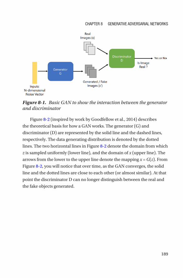
189
Figure 8-2 (inspired by work by Goodfellow et al., 2014) describes
the theoretical basis for how a GAN works. The generator (G) and
discriminator (D) are represented by the solid line and the dashed lines,
respectively. The data generating distribution is denoted by the dotted
lines. The two horizontal lines in Figure 8-2 denote the domain from which
z is sampled uniformly (lower line), and the domain of x (upper line). The
arrows from the lower to the upper line denote the mapping x = G(z). From
Figure 8-2, you will notice that over time, as the GAN converges, the solid
line and the dotted lines are close to each other (or almost similar). At that
point the discriminator D can no longer distinguish between the real and
the fake objects generated.
Figure 8-1. Basic GAN to show the interaction between the generator and discriminator
Chapter 8 Generative adversarial networks

190
In the early version of GANs, the generator and the discriminator
are implemented as fully connected neural networks (Goodfellow et al.,
2014). These GANs are used for generating images from various data sets
commonly used in deep learning: CIFAR10, MNIST (handwritten digits),
and the Toronto Face Dataset, for example. As the architecture of GANs has
evolved, CNNs are increasingly being used. An example of a GAN that uses
deep CNNs is DCGANs (Radford, Metz, & Chintala, 2016). A comprehensive
overview of different types of GANs can be found in Creswell et al. (2017).
Since 2014, very innovative approaches to using GANs have emerged.
GANs have shown promise in the use of AI for creativity, such as art
and music generation and computer-aided design (CAD). One of these
approaches is to automate the generation of images using text descriptions.
InfoGAN (Chen et al., 2016) is an unsupervised approach that can distill
the semantic and hidden representations from several well-known data
sets (e.g., Digits [MNIST], CelebA Faces, and House Numbers [SVHN]). The
secret behind InfoGAN is maximizing the mutual information between
latent variables and the observations. The stacked Generative Adversarial
Networks (StackGAN; Zhang et al., 2016) was proposed to generate
photorealistic images using text descriptions. For example, given the text
Figure 8-2. How GANs work: The generator is generating objects that are so real that the discriminator can no longer tell the difference between real and fake. Source: Goodfellow et al. (2014).
Chapter 8 Generative adversarial networks

191
“This bird has a yellow belly and tarsus, grey back, wings, and brown throat,
nape with a black face,” StackGAN will generate the picture of a bird using
two stages. In Stage 1, a low-resolution image is computed, which consists
of basic shapes and colors. In Stage 2, the results from Stage 1 and the text
descriptions are used to create photorealistic high-resolution images.
Figure 8-3 shows the two stages of the StackGAN.
Figure 8-3. StackGAN: Generation of image from text. Source: Zhang et al. (2016).
Like StackGAN, Attentional Generative Adversarial Network
(AttnGAN) uses a multistage approach. In addition, AttnGan introduced
a novel attention-driven approach that focuses (or pays attention) to the
different words in the text description and uses this to synthesize fine-
grained details for each of the subregions of an image. Figure 8-4 shows
how AttnGAN works, and the different parts of the image that it is focusing
on for the different words. The first row shows the image generated by
different generators, each producing images of different dimension (from
64 × 64, to 128 × 128, to 256 × 256). The second and third row show the top
five most attended words (i.e., words with the highest values as defined by
each attention model).
Chapter 8 Generative adversarial networks
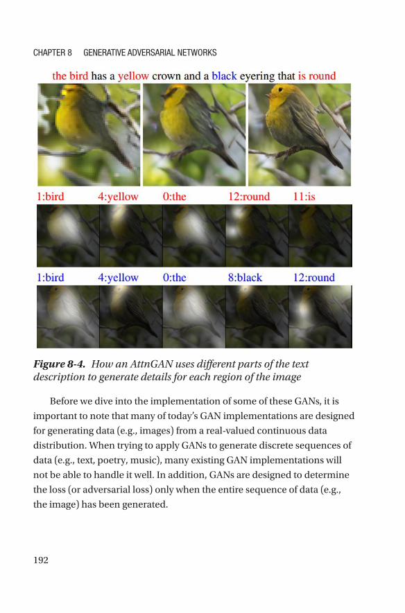
192
Before we dive into the implementation of some of these GANs, it is
important to note that many of today’s GAN implementations are designed
for generating data (e.g., images) from a real-valued continuous data
distribution. When trying to apply GANs to generate discrete sequences of
data (e.g., text, poetry, music), many existing GAN implementations will
not be able to handle it well. In addition, GANs are designed to determine
the loss (or adversarial loss) only when the entire sequence of data (e.g.,
the image) has been generated.
Figure 8-4. How an AttnGAN uses different parts of the text description to generate details for each region of the image
Chapter 8 Generative adversarial networks
193
Another interesting type of GAN is SeqGAN (Yu, Zhang, Wang, &
Yu, n.d.). SeqGAN is a novel approach toward integrating reinforcement
learning concepts into GANs to overcome the various challenges faced
by existing GANs when used to generate discrete sequences of data. In
a SeqGAN, the generator is designed to be an agent of reinforcement
learning, where its current state is the generated discrete tokens so far, and
the action is the next token to be generated. The discriminator evaluates
the generated tokens and provides feedback to help the generator to learn.
SeqGAN is shown to be effective in poetry generation, music generation,
and application to language and speech tasks.
Today, GANs work well for several types of problems, but they are
notoriously difficult to train, as they are not guaranteed to converge on
a solution that is optimal, or even stable. Another common issue with
GANs is known as mode collapse, where the generator creates samples
that have extremely low variety. They require very careful selection of the
hyperparameters and parameter initialization among other factors to work
well. At the 2016 NIPS workshop on adversarial training, for example,
how to explain and fix the issues in training GANs was a main topic (video
recordings can be watched at http://bit.ly/NIPS2016). Fortunately,
though, many tricks have been used to stabilize the training of GANs.
One such trick is to include additional information either in the input
space (e.g., adding continuous noise to the input of the discriminator) or
adding the information to the output space (e.g., different classes of true
examples). Other tricks look at introducing a regularization scheme during
training.
Note learn about the evolution of Gans at http://bit.ly/GANsEvolve.
Chapter 8 Generative adversarial networks
194
This chapter walks through one of the GANs, known as Cycle-
Consistent Adversarial Networks (CycleGANs). We learn how CycleGANs
can be used for image-to-image translation. By walking through the
code, we will jump start our understanding of GANs and the innovative
applications of GANs in your AI projects. You can leverage the Microsoft
AI Platform to train and deploy these GANs to the cloud, mobile, and edge
devices.
Cycle-Consistent Adversarial NetworksCycleGANs are a novel approach for translating an image from a source
domain X to a target domain Y. One of the strengths of CycleGANs is that
the training of the GAN does not require the training data to have matching
image pairs. As noted in Zhu, Park, Isola, and Efros (2017), CycleGANs
have been successfully applied in the following use cases:
• Translating Monet paintings to photos.
• Style transfer for photos using styles from various
famous artists (Monet, Van Gogh, Cezanne, and
Ukiyo-e).
• Object transfiguration, where it is used for changing the
type of objects found in photos. Figure 8-5 shows how
CycleGANs are used in object transfiguration (horse to
zebra, zebra to horse, apple to orange, orange to apple,
etc.).
• Translating a photo from one season (e.g., summer) to
another (e.g., winter).
• Photo enhancement by narrowing the depth of field,
and more.
Chapter 8 Generative adversarial networks

195
The goal of CycleGANs is to learn how to map images from one domain
X to another domain Y. Figure 8-6 shows the use of two mapping functions
G and F, and two discriminators DX and DY. The discriminator DX is used
to verify the images from X and the translated images F(y). Similarly, the
discriminator DY is used to verify the images from Y and the translated
images G(x). The secret behind the effectiveness of using CycleGANs for
image translation is the use of a cycle consistency loss. Intuitively, the cycle
consistency loss is used to determine whether images from the domain X
can be recovered from the translated image.
Figure 8-5. Object transfiguration (horse to zebra, apple to orange). Source: Zhu, Park, Isola, and Efros (2017).
Figure 8-6. CycleGANs model with two mapping functions G and F, and two adversarial discriminators DX and DY
Chapter 8 Generative adversarial networks

196
Note CycleGans were first introduced in Zhu et al. (2017). the original implementation of CycleGans (in pytorch) is available at http://bit.ly/CycleGAN.
The CycleGAN CodeLet us first walk through the overall CycleGAN code that will be used for
training the CycleGANs and then testing it by translating images from a
source domain A to a target domain B. For example, the trained CycleGAN
will perform object transfiguration and translate a photo consisting of
a horse to a zebra (and vice versa). The results are then visualized as an
HTML file.
Let us first import the Python libraries that we will use in this code.
From Listing 8-1, you will see that we are using TensorFlow, and importing
the definition of the CycleGAN from a model.py file. We will dive into the
details of the model.py fie in the later parts of this section.
Note we recommend provisioning an azure dlvM to run the code examples in this chapter. please see Chapter 4 for more information.
Listing 8-1. Importing the Required Python Libraries
PYTHON
import os
import tensorflow as tf
from model import cyclegan
Next, we define the argument that will be used for training and testing
the CycleGAN. From Listing 8-2, you will see that we specified a learning
rate of 0.0002 for 200 epochs (denoted by lr and epoch_step). In addition,
Chapter 8 Generative adversarial networks
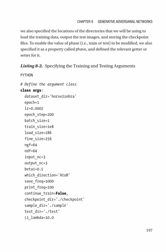
197
we also specified the locations of the directories that we will be using to
load the training data, output the test images, and storing the checkpoint
files. To enable the value of phase (i.e., train or test) to be modified, we also
specified it as a property called phase, and defined the relevant getter or
setter for it.
Listing 8-2. Specifying the Training and Testing Arguments
PYTHON
# Define the argument class
class args:
dataset_dir='horse2zebra'
epoch=1
lr=0.0002
epoch_step=200
batch_size=1
train_size=1e8
load_size=286
fine_size=256
ngf=64
ndf=64
input_nc=3
output_nc=3
beta1=0.5
which_direction='AtoB'
save_freq=1000
print_freq=100
continue_train=False,
checkpoint_dir='./checkpoint'
sample_dir='./sample'
test_dir='./test'
L1_lambda=10.0
Chapter 8 Generative adversarial networks
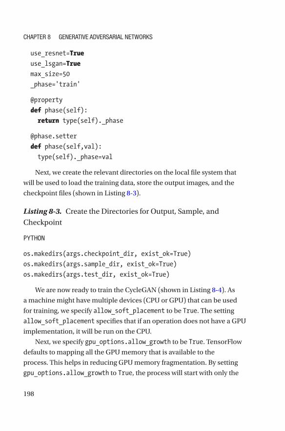
198
use_resnet=True
use_lsgan=True
max_size=50
_phase='train'
@property
def phase(self):
return type(self)._phase
@phase.setter
def phase(self,val):
type(self)._phase=val
Next, we create the relevant directories on the local file system that
will be used to load the training data, store the output images, and the
checkpoint files (shown in Listing 8-3).
Listing 8-3. Create the Directories for Output, Sample, and
Checkpoint
PYTHON
os.makedirs(args.checkpoint_dir, exist_ok=True)
os.makedirs(args.sample_dir, exist_ok=True)
os.makedirs(args.test_dir, exist_ok=True)
We are now ready to train the CycleGAN (shown in Listing 8-4). As
a machine might have multiple devices (CPU or GPU) that can be used
for training, we specify allow_soft_placement to be True. The setting
allow_soft_placement specifies that if an operation does not have a GPU
implementation, it will be run on the CPU.
Next, we specify gpu_options.allow_growth to be True. TensorFlow
defaults to mapping all the GPU memory that is available to the
process. This helps in reducing GPU memory fragmentation. By setting
gpu_options.allow_growth to True, the process will start with only the
Chapter 8 Generative adversarial networks
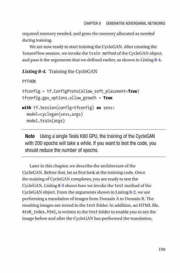
199
required memory needed, and grow the memory allocated as needed
during training.
We are now ready to start training the CycleGAN. After creating the
TensorFlow session, we invoke the train method of the CycleGAN object,
and pass it the arguments that we defined earlier, as shown in Listing 8-4.
Listing 8-4. Training the CycleGAN
PYTHON
tfconfig = tf.ConfigProto(allow_soft_placement=True)
tfconfig.gpu_options.allow_growth = True
with tf.Session(config=tfconfig) as sess:
model=cyclegan(sess,args)
model.train(args)
Note Using a single tesla k80 GpU, the training of the CycleGan with 200 epochs will take a while. if you want to test the code, you should reduce the number of epochs.
Later in this chapter, we describe the architecture of the
CycleGAN. Before that, let us first look at the training code. Once
the training of CycleGAN completes, you are ready to test the
CycleGAN. Listing 8-5 shows how we invoke the test method of the
CycleGAN object. From the arguments shown in Listing 8-2, we are
performing a translation of images from Domain A to Domain B. The
resulting images are stored in the test folder. In addition, an HTML file,
AtoB_index.html, is written to the test folder to enable you to see the
image before and after the CycleGAN has performed the translation.
Chapter 8 Generative adversarial networks
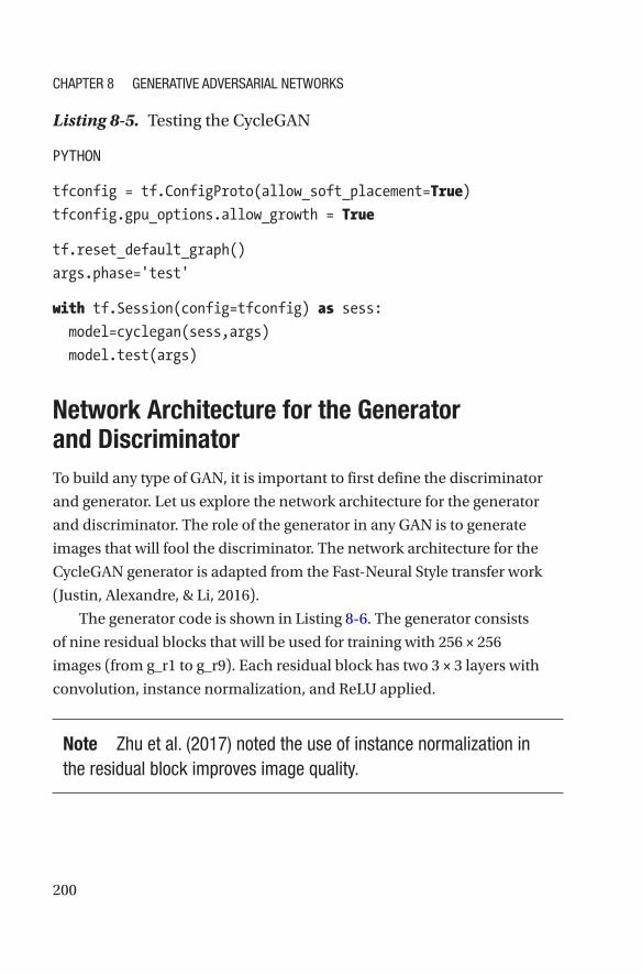
200
Listing 8-5. Testing the CycleGAN
PYTHON
tfconfig = tf.ConfigProto(allow_soft_placement=True)
tfconfig.gpu_options.allow_growth = True
tf.reset_default_graph()
args.phase='test'
with tf.Session(config=tfconfig) as sess:
model=cyclegan(sess,args)
model.test(args)
Network Architecture for the Generator and DiscriminatorTo build any type of GAN, it is important to first define the discriminator
and generator. Let us explore the network architecture for the generator
and discriminator. The role of the generator in any GAN is to generate
images that will fool the discriminator. The network architecture for the
CycleGAN generator is adapted from the Fast-Neural Style transfer work
(Justin, Alexandre, & Li, 2016).
The generator code is shown in Listing 8-6. The generator consists
of nine residual blocks that will be used for training with 256 × 256
images (from g_r1 to g_r9). Each residual block has two 3 × 3 layers with
convolution, instance normalization, and ReLU applied.
Note Zhu et al. (2017) noted the use of instance normalization in the residual block improves image quality.
Chapter 8 Generative adversarial networks
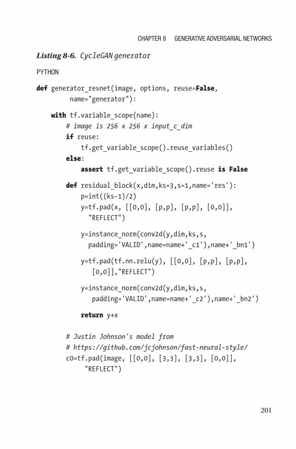
201
Listing 8-6. CycleGAN generator
PYTHON
def generator_resnet(image, options, reuse=False,
name="generator"):
with tf.variable_scope(name):
# image is 256 x 256 x input_c_dim
if reuse:
tf.get_variable_scope().reuse_variables()
else:
assert tf.get_variable_scope().reuse is False
def residual_block(x,dim,ks=3,s=1,name='res'):
p=int((ks-1)/2)
y=tf.pad(x, [[0,0], [p,p], [p,p], [0,0]],
"REFLECT")
y=instance_norm(conv2d(y,dim,ks,s,
padding='VALID',name=name+'_c1'),name+'_bn1')
y=tf.pad(tf.nn.relu(y), [[0,0], [p,p], [p,p],
[0,0]],"REFLECT")
y=instance_norm(conv2d(y,dim,ks,s,
padding='VALID',name=name+'_c2'),name+'_bn2')
return y+x
# Justin Johnson's model from
# https://github.com/jcjohnson/fast-neural-style/
c0=tf.pad(image, [[0,0], [3,3], [3,3], [0,0]],
"REFLECT")
Chapter 8 Generative adversarial networks
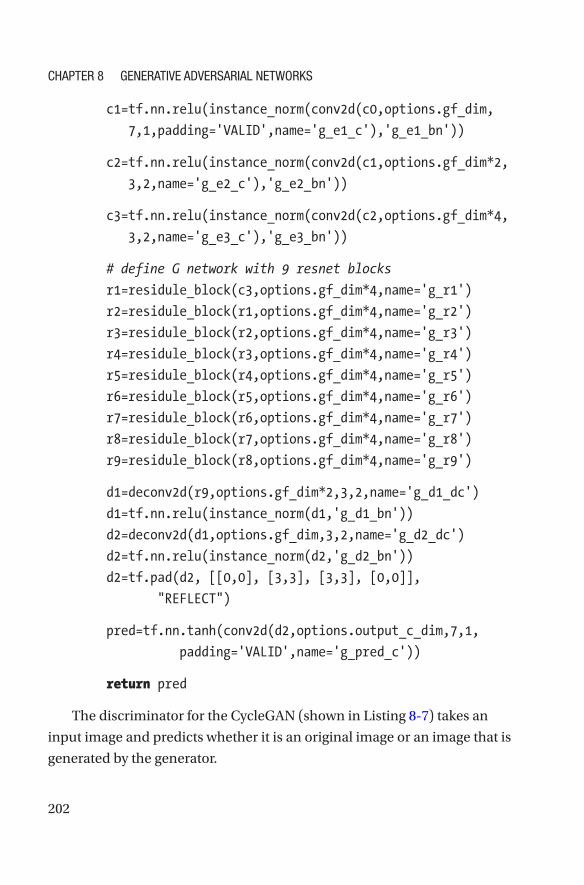
202
c1=tf.nn.relu(instance_norm(conv2d(c0,options.gf_dim,
7,1,padding='VALID',name='g_e1_c'),'g_e1_bn'))
c2=tf.nn.relu(instance_norm(conv2d(c1,options.gf_dim*2,
3,2,name='g_e2_c'),'g_e2_bn'))
c3=tf.nn.relu(instance_norm(conv2d(c2,options.gf_dim*4,
3,2,name='g_e3_c'),'g_e3_bn'))
# define G network with 9 resnet blocks
r1=residule_block(c3,options.gf_dim*4,name='g_r1')
r2=residule_block(r1,options.gf_dim*4,name='g_r2')
r3=residule_block(r2,options.gf_dim*4,name='g_r3')
r4=residule_block(r3,options.gf_dim*4,name='g_r4')
r5=residule_block(r4,options.gf_dim*4,name='g_r5')
r6=residule_block(r5,options.gf_dim*4,name='g_r6')
r7=residule_block(r6,options.gf_dim*4,name='g_r7')
r8=residule_block(r7,options.gf_dim*4,name='g_r8')
r9=residule_block(r8,options.gf_dim*4,name='g_r9')
d1=deconv2d(r9,options.gf_dim*2,3,2,name='g_d1_dc')
d1=tf.nn.relu(instance_norm(d1,'g_d1_bn'))
d2=deconv2d(d1,options.gf_dim,3,2,name='g_d2_dc')
d2=tf.nn.relu(instance_norm(d2,'g_d2_bn'))
d2=tf.pad(d2, [[0,0], [3,3], [3,3], [0,0]],
"REFLECT")
pred=tf.nn.tanh(conv2d(d2,options.output_c_dim,7,1,
padding='VALID',name='g_pred_c'))
return pred
The discriminator for the CycleGAN (shown in Listing 8-7) takes an
input image and predicts whether it is an original image or an image that is
generated by the generator.
Chapter 8 Generative adversarial networks

203
Listing 8-7. CycleGAN Discriminator
PYTHON
def discriminator(image, options, reuse=False,
name="discriminator"):
with tf.variable_scope(name):
# image is 256 x 256 x input_c_dim
if reuse:
tf.get_variable_scope().reuse_variables()
else:
assert tf.get_variable_scope().reuse is False
h0=lrelu(conv2d(image,options.df_dim,
name='d_h0_conv'))
# h0 is (128 x 128 x self.df_dim)
h1=lrelu(instance_norm(conv2d(h0,options.df_dim*2,
name='d_h1_conv'),'d_bn1'))
# h1 is (64 x 64 x self.df_dim*2)
h2=lrelu(instance_norm(conv2d(h1,options.df_dim*4,
name='d_h2_conv'),'d_bn2'))
# h2 is (32x 32 x self.df_dim*4)
h3=lrelu(instance_norm(conv2d(h2,options.df_dim*8,s=1,
name='d_h3_conv'),'d_bn3'))
# h3 is (32 x 32 x self.df_dim*8)
h4=conv2d(h3,1,s=1,name='d_h3_pred')
# h4 is (32 x 32 x 1)
return h4
Chapter 8 Generative adversarial networks
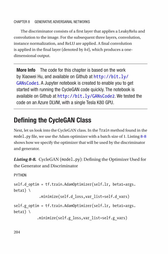
204
The discriminator consists of a first layer that applies a LeakyRelu and
convolution to the image. For the subsequent three layers, convolution,
instance normalization, and ReLU are applied. A final convolution
is applied in the final layer (denoted by h4), which produces a one-
dimensional output.
More Info the code for this chapter is based on the work by Xiaowei hu, and available on Github at http://bit.ly/GANsCode1. a Jupyter notebook is created to enable you to get started with running the CycleGan code quickly. the notebook is available on Github at http://bit.ly/GANsCode2. we tested the code on an azure dlvM, with a single tesla k80 GpU.
Defining the CycleGAN ClassNext, let us look into the CycleGAN class. In the Train method found in the
model.py file, we use the Adam optimizer with a batch size of 1. Listing 8-8
shows how we specify the optimizer that will be used by the discriminator
and generator.
Listing 8-8. CycleGAN (model.py): Defining the Optimizer Used for
the Generator and Discriminator
PYTHON
self.d_optim = tf.train.AdamOptimizer(self.lr, beta1=args.
beta1) \
.minimize(self.d_loss,var_list=self.d_vars)
self.g_optim = tf.train.AdamOptimizer(self.lr, beta1=args.
beta1) \
.minimize(self.g_loss,var_list=self.g_vars)
Chapter 8 Generative adversarial networks
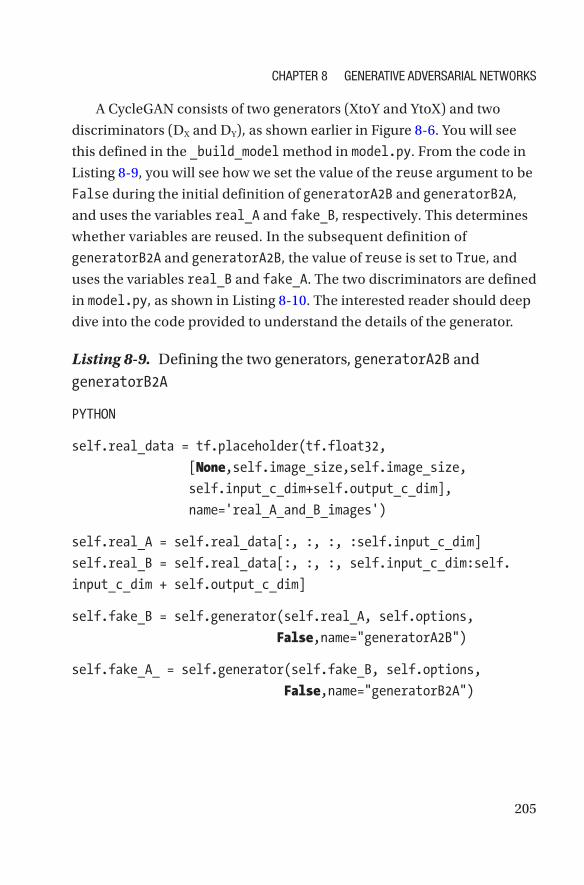
205
A CycleGAN consists of two generators (XtoY and YtoX) and two
discriminators (DX and DY), as shown earlier in Figure 8-6. You will see
this defined in the _build_model method in model.py. From the code in
Listing 8-9, you will see how we set the value of the reuse argument to be
False during the initial definition of generatorA2B and generatorB2A,
and uses the variables real_A and fake_B, respectively. This determines
whether variables are reused. In the subsequent definition of
generatorB2A and generatorA2B, the value of reuse is set to True, and
uses the variables real_B and fake_A. The two discriminators are defined
in model.py, as shown in Listing 8-10. The interested reader should deep
dive into the code provided to understand the details of the generator.
Listing 8-9. Defining the two generators, generatorA2B and
generatorB2A
PYTHON
self.real_data = tf.placeholder(tf.float32,
[None,self.image_size,self.image_size,
self.input_c_dim+self.output_c_dim],
name='real_A_and_B_images')
self.real_A = self.real_data[:, :, :, :self.input_c_dim]
self.real_B = self.real_data[:, :, :, self.input_c_dim:self.
input_c_dim + self.output_c_dim]
self.fake_B = self.generator(self.real_A, self.options,
False,name="generatorA2B")
self.fake_A_ = self.generator(self.fake_B, self.options,
False,name="generatorB2A")
Chapter 8 Generative adversarial networks
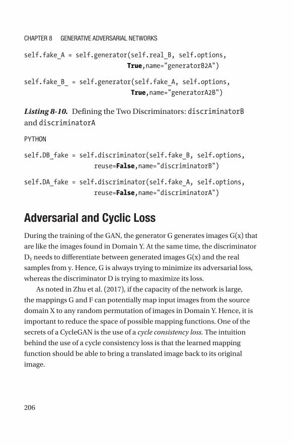
206
self.fake_A = self.generator(self.real_B, self.options,
True,name="generatorB2A")
self.fake_B_ = self.generator(self.fake_A, self.options,
True,name="generatorA2B")
Listing 8-10. Defining the Two Discriminators: discriminatorB
and discriminatorA
PYTHON
self.DB_fake = self.discriminator(self.fake_B, self.options,
reuse=False,name="discriminatorB")
self.DA_fake = self.discriminator(self.fake_A, self.options,
reuse=False,name="discriminatorA")
Adversarial and Cyclic LossDuring the training of the GAN, the generator G generates images G(x) that
are like the images found in Domain Y. At the same time, the discriminator
DY needs to differentiate between generated images G(x) and the real
samples from y. Hence, G is always trying to minimize its adversarial loss,
whereas the discriminator D is trying to maximize its loss.
As noted in Zhu et al. (2017), if the capacity of the network is large,
the mappings G and F can potentially map input images from the source
domain X to any random permutation of images in Domain Y. Hence, it is
important to reduce the space of possible mapping functions. One of the
secrets of a CycleGAN is the use of a cycle consistency loss. The intuition
behind the use of a cycle consistency loss is that the learned mapping
function should be able to bring a translated image back to its original
image.
Chapter 8 Generative adversarial networks

207
ResultsAfter we ran the CycleGAN training for 150 epochs, we ran the testing
code shown in Listing 8-5. This applies the CycleGAN model to the images
found in the dataset directory and output the translated image to the test
directory. An HTML file is also generated. This allows you to visualize the
original and the translated image side by side. In the Jupyter notebook
provided, the code (shown in Listing 8-11) enables the HTML file to be
viewed in a notebook cell.
Listing 8-11. Python Code to Visualize HTML File in the Cell
PYTHON
from IPython.display import HTML
HTML(filename='test/AtoB_index.html')
In Figure 8-7, we show a subset of the images generated.
Figure 8-7. Output from CycleGAN test (after 150 epochs)
Chapter 8 Generative adversarial networks
208
SummaryGANs have tremendous potential to be used in AI for creativity, music,
and the arts. Since it was first proposed in 2014, GANs innovations are
happening at a breathtaking pace. This chapter described how GANs can
be applied to various use cases. We showed the use of the generator and
the discriminator in the GAN architecture, and how they are used.
Next, we discussed how CycleGAN works, and showed how it can be
used for translation of objects from one domain to another. In the code
example given in this chapter, we focus on how to train and test a novel
type of GAN, called CycleGAN.
All the code in this chapter is run on a Linux DLVM, available on Azure.
More details on choices for training AI models (e.g., GANs), such as the
computing environments and how to do training at scale, are discussed in
the next chapter.
Chapter 8 Generative adversarial networks
PART IV
AI Architectures and Best Practices
211© Mathew Salvaris, Danielle Dean, Wee Hyong Tok 2018 M. Salvaris et al., Deep Learning with Azure, https://doi.org/10.1007/978-1-4842-3679-6_9
CHAPTER 9
Training AI ModelsTraining AI models is usually more demanding than training standard
ML models because they are processing intensive and often the data sets
involved are larger. That is why if you are serious about deep learning you
have to have access to GPUs. In Azure there are a number of ways you
can make use of GPUs, on single VMs or in orchestrated clusters of them.
In this chapter, we summarize several of the most common methods
available as well as the pros and cons of each. Then we expand on the code
we wrote in Chapter 6, which used a VGG-like CNN to tackle the CIFAR10
data set using the DLVM as the computing environment. In this chapter,
we extend to other training options such as Batch AI and Batch Shipyard,
which can both be useful for scaling up or scaling out training. We finish
by highlighting briefly some of the other methods of training AI models
on Azure that are not as common but might be useful depending on the
problem at hand.
Training OptionsAzure has a vast number of options for training AI models. We will limit
ourselves here to the select few that we feel fulfill the requirements of most
workload types. The four ways that we discuss to train AI models are DLVM,
Batch AI, Batch Shipyard, and DL Workspace. There is no best way to train
an AI model; each method has its benefits and drawbacks and some will be
more suited to certain solutions than others. The training of a deep learning

212
model can take place on a single GPU machine or distributed across a
number of GPU machines. The most common scenario is to use a single
GPU machine per model, as training the model in a distributed fashion
needs additional considerations that can be quite tricky to get right but
might be necessitated by factors such as the model being too big to fit onto a
single GPU machine or wanting to reduce training time.
In this chapter, we do not mention the data processing that is often
needed before training an AI model. For example, the raw data will often
have to be processed to be readable by a deep learning model, the labels
on which the ML algorithm should learn might be stored in a database, or
the raw data might come from many sources. There are many tools and
options available within the Microsoft AI Platform for this type of work,
such as Azure SQL Data Warehouse and CosmosDB for storing different
types of data, and Azure Data Factory for data movement, which are
outside the scope of this chapter. We assume for purposes here that the
data are available in a format that is ready to be trained by an AI model.
Distributed TrainingDistributed training is used when the whole data set cannot be stored on a
single machine or the model cannot fit on a single GPU, but most often it is
used to achieve faster training. The two main types of distributed training
are data parallelism or model parallelism.
With data parallelism, the same model will be replicated across many
GPUs and will receive different batches of training data. The gradients are
then aggregated and then the updates distributed back to the models. In
this scenario the communication overhead can be quite substantial so
an active area of exploration is how to make this process more efficient
by exploring asynchronous updates (Calauzènes & Roux, 2017; Dean
et al., 2012; Recht, Re, Wright, & Niu, 2011) or reducing the overhead by
compressing or quantizing the weight updates (Lin, Han, Mao, Wang, &
Dally, 2017; Recht et al., 2011).
Chapter 9 training ai Models
213
With model parallelism the model is split over multiple GPUs. An
example of this might be different layers placed on different GPUs
and the forward and backward passes over the model involve network
communication across the nodes. This is a far less common scenario and
is only necessary if the model cannot fit on a single GPU.
In these scenarios it is assumed that there is only one GPU per VM, often
referred to as multinode multi-GPU, but in fact Azure has configurations
where there can be up to four GPUs on a single VM. All of the scenarios just
explained can be executed on a single-node multi-GPU scenario except the
scenario where the data are too large to fit on a single VM. Communication
overhead is usually less of a concern in this scenario because it takes place
on a single node and can perform even better if the deep learning framework
uses Nvidia’s NCCL multi-GPU library (http://bit.ly/nvidianccl).
Deep Learning Virtual MachineThe DLVM is a single VM that comes in a number of different
configurations, some of which have GPUs, and is a specially configured
variant of the DSVM. The VM types that have GPUs at the moment are NC,
NV, ND, NCv2, and NCv3, with the cheapest being the NC series. These
have the corresponding GPUs installed with NVIDIA Tesla K80, M60, P40,
P100, and finally V100. They are loosely ordered from the least powerful to
the most powerful, with a single K80 providing around 4.4 teraflops and a
single V100 offering around 14 teraflops.1
Note even the least powerful gpU (K80) provides significant reductions in training time compared to training ai models on CpUs.
1 Order and numbers are based on single precision FLOPS; cards with two chips are treated as individual GPUs.
Chapter 9 training ai Models
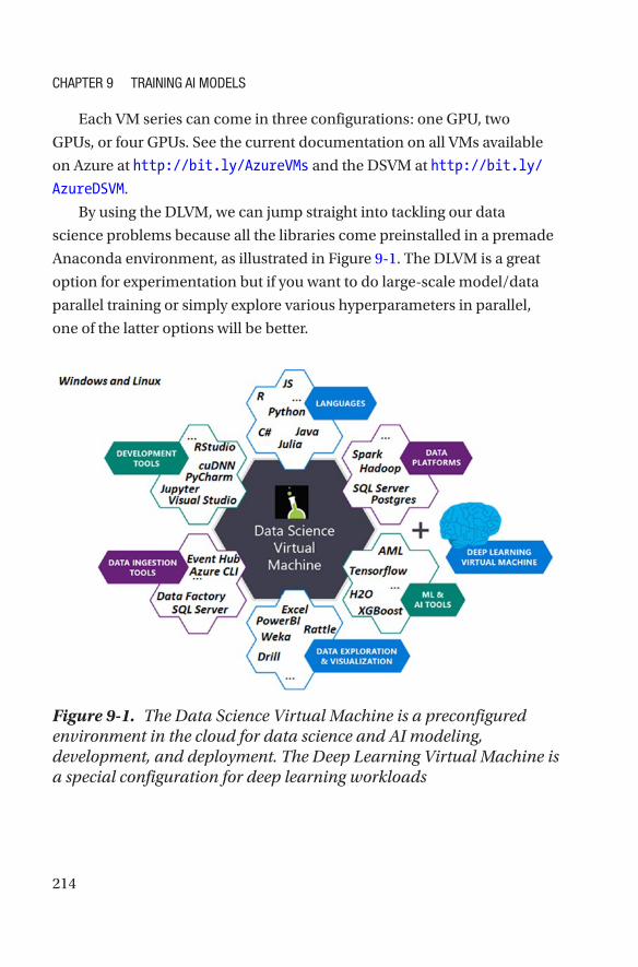
214
Each VM series can come in three configurations: one GPU, two
GPUs, or four GPUs. See the current documentation on all VMs available
on Azure at http://bit.ly/AzureVMs and the DSVM at http://bit.ly/
AzureDSVM.
By using the DLVM, we can jump straight into tackling our data
science problems because all the libraries come preinstalled in a premade
Anaconda environment, as illustrated in Figure 9-1. The DLVM is a great
option for experimentation but if you want to do large-scale model/data
parallel training or simply explore various hyperparameters in parallel,
one of the latter options will be better.
Figure 9-1. The Data Science Virtual Machine is a preconfigured environment in the cloud for data science and AI modeling, development, and deployment. The Deep Learning Virtual Machine is a special configuration for deep learning workloads
Chapter 9 training ai Models

215
Batch ShipyardBatch Shipyard is a general-purpose tool for running container-based
batch processing and High Performance Computing (HPC) workloads.
By building on top of Azure Batch, Batch Shipyard is able to benefit from
its features, such as handling the complexities surrounding large-scale
parallel and HPC applications in the cloud, managing aspects such as
the VM deployment and management, job scheduling, and autoscaling
requirements. There is no extra cost to use Azure Batch when running jobs
on Azure; it is a free, value-added service where costs are only incurred for
the computing resources consumed and related datacenter movement and
storage costs.
Batch Shipyard uses Docker containers, which makes it easy to manage
the complex dependencies that come with AI workloads. Batch Shipyard
is available as a CLI that can be run locally or in the cloud using the Azure
Cloud Shell. The orchestration is managed through easy-to-understand
configuration files, which makes it easy to reuse scripts. It already contains
a large number of examples for some of the most popular deep learning
frameworks (see http://bit.ly/shipyard24c3).
The following are some of the pros of using Batch Shipyard:
• It is tied to Azure Batch infrastructure so it is well
supported.
• It is easy to use from the CLI and also available in the
cloud shell.
• It supports many different types of VMs, including
GPUs.
• It supports low-priority nodes, which makes it very
efficient.
• It has factory methods to support easy hyperparameter
tuning.
Chapter 9 training ai Models
216
Among the disadvantages of using Batch Shipyard are the following:
• It is tied to Batch infrastructure, so there is no support
for its own clusters.
• There is no REST API or web front end, only the CLI.
Batch AIBatch AI is very similar to Batch Shipyard, as it runs on Azure Batch and
allows you to run various AI workloads. The core differences between
Batch Shipyard and Batch AI are the following:
1. It is a managed service. This means that with Batch
Shipyard the CLI is calling out to Azure Batch
and setting everything up. With Batch AI there is
a service in the cloud that we call to use the CLI,
REST API, or SDK, and it orchestrates everything.
In practice, this means is there is a far richer way to
interact with Batch AI and it is easier to orchestrate
as part of a pipeline.
2. Batch AI can execute on a DSVM or DLVM, giving
it the ability to run things without containers. This
makes it very easy to get started if you do not want to
deal with the complexities of containers.
3. Batch AI provides specialized support for running
distributed training on a number of deep learning
frameworks such as PyTorch, TensorFlow, and
so on. In practice, this means that some of the
complexities such as setting up Message Passing
Interface (MPI) are automatically configured by
Batch AI.
Chapter 9 training ai Models
217
These are some of the pros of Batch AI:
• It is a managed service.
• It has multiple ways to interact with the CLI, SDK, and
REST APIs.
• It is tied to Azure Batch infrastructure so it is well supported.
• It supports many different types of VM including GPUs.
• It supports low-priority nodes that are very cost- efficient.
• It can support DSVM and DLVM as computing targets.
The following are some of the disadvantages of using Batch AI:
• It does not have feature parity with Batch Shipyard.
Batch Shipyard offers some nice methods for
hyperparameter search that have not yet made their
way to Batch AI.
• It is still in previews and not available in all regions.
Deep Learning WorkspaceDeep Learning Workspace (DLWorkspace) is an open source project from
Microsoft that allows AI scientists to spin up clusters, either locally or in
the cloud, in a turn-key fashion. DLWorkspace uses Kubernetes to manage
the jobs across the various nodes. Kubernetes is a popular open source
container orchestrator and we will talk more about it in Chapter 10.
DLWorkspace provides a web user interface (UI) and a REST API from
which one can submit, monitor, and manage jobs. This is quite different
from Batch AI and Batch Shipyard, as it does not rely on the Batch
infrastructure to manage things, nor is it tied to the Azure infrastructure.
This does mean it requires more management by the end user than the
other two options, but it offers the greatest amount of flexibility. It is also
less mature than the other two options.
Chapter 9 training ai Models
218
The following are some of the advantages of DLWorkspace:
• It is not tied to a particular infrastructure, so it can run
on local clusters and in the cloud.
• It uses Kubernetes, a well-known container
orchestrator.
Some of the disadvantages of DLWorkspace are as follows:
• It requires more setup than Batch Shipyard or Batch AI.
• It is harder to integrate into a pipeline.
• It is still under heavy development.
Examples to Follow AlongIn many of the previous chapters we have demonstrated how to train a
deep learning model on a GPU-enabled DLVM, so we do not go over that
here. In the sections that immediately follow, we will be making use of
the code we wrote in Chapter 6, which used a VGG-like CNN to tackle the
CIFAR10 data set, to expand to use Batch Shipyard and Batch AI. If you
do not remember what we did there, it would be prudent to go back and
refresh your memory.
Training DNN on Batch ShipyardIn this section we go over general steps of how to train a CNN on Batch
Shipyard. The steps that we follow to execute our AI script are detailed in
the notebook Chapter_09_01.ipynb2 and shown in Figure 9-2.
2 All the steps are detailed in the notebook Chapter_09_01.ipynb which can be found in the Chapter_09 folder http://bit.ly/CH09Notebooks.
Chapter 9 training ai Models
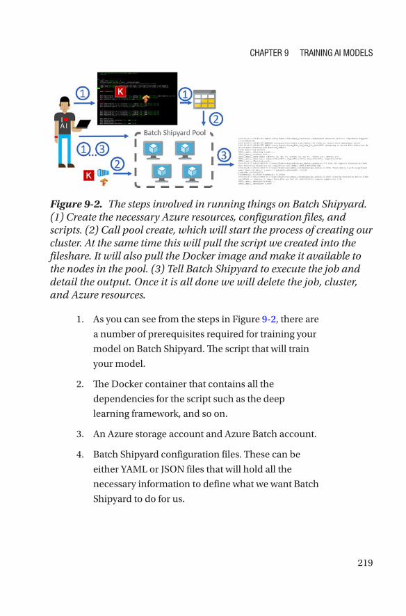
219
1. As you can see from the steps in Figure 9-2, there are
a number of prerequisites required for training your
model on Batch Shipyard. The script that will train
your model.
2. The Docker container that contains all the
dependencies for the script such as the deep
learning framework, and so on.
3. An Azure storage account and Azure Batch account.
4. Batch Shipyard configuration files. These can be
either YAML or JSON files that will hold all the
necessary information to define what we want Batch
Shipyard to do for us.
Figure 9-2. The steps involved in running things on Batch Shipyard. (1) Create the necessary Azure resources, configuration files, and scripts. (2) Call pool create, which will start the process of creating our cluster. At the same time this will pull the script we created into the fileshare. It will also pull the Docker image and make it available to the nodes in the pool. (3) Tell Batch Shipyard to execute the job and detail the output. Once it is all done we will delete the job, cluster, and Azure resources.
Chapter 9 training ai Models

220
Our model script will be very similar to what we wrote in the
Chapter_06_03.ipynb notebook, except it will be a Python file rather than
a Jupyter notebook and we will add the ability to pass arguments to it. The
reason for doing this is to simplify the execution and so that we can see
how the model performs with different hyperparameter configurations.
This is usually referred to as hyperparameter search and it is an important
step in creating AI models. The script will download the CIFAR10 data,
create and train our model, and finally evaluate it on the test data set.
With the script prepared, we need to either create our own Docker
image or reference a prebuilt one. Many of the most popular deep learning
frameworks either provide you with a Docker image or at the very least a
Dockerfile you can use to create your image. For people who have not
used Docker before, this can be quite daunting. Thankfully there are a
number of guides online and the Docker documentation is very good
(see http://bit.ly/dockerstarted). Here we simply use the Docker
image we created for this book.
We will assume that you have created the Azure storage and Batch
account. The steps for doing this are outlined in the “Create Azure
Resources” section of the accompanying notebook. For Batch Shipyard
there are four configuration files:
• credentials.yaml: Here we put the credentials for all
the resources we use. In our case it is simply the storage
account and Batch account.
• config.yaml: Specifies the configuration for Batch
Shipyard. Here we will simply specify which storage
account to use as well as the location of the image we
want to use.
• pool.yaml: This configuration file defines the properties
of our pool, in essence the number of VMs we want to
allocate and the types of VMs we wish to allocate.
Chapter 9 training ai Models

221
• jobs.yaml: In this configuration file we specify the
jobs we wish to execute. We can specify one or more
jobs and each job can have one or more tasks. How
you split things up will be dependent on the tasks you
want to run and how much they share in common. In
this file we generally specify what Docker image to use,
where to ingress the data from, and what commands
to execute. For more details see http://bit.ly/
shipyardjobs.
From here on in we will be assuming you are running things from
a Linux terminal or a Jupyter notebook running on Linux. Now that we
have defined our configuration files and our script, we need to create our
cluster, which we do in Listing 9-1.
Listing 9-1. Command to Create a Batch Cluster
BASH
shipyard pool add --configdir config
This command tells Batch Shipyard to create the pool as specified in
our pool.yaml file located in the config directory. This will start the VMs
and ingress any files we specified in the configuration files, which in our
case is just our model script. Provisioning the pool can take from 5 to 15
minutes depending on the number of VMs specified. The number of VMs
you can create is dependent on the quota on your Batch account. If you
require more VMs for your Batch account, you can simply request a quota
increase through the Azure portal (http://bit.ly/azbatchquota).
After the pool has been created, we simply add the jobs. Here in
Listing 9-2 we submit the job but also interactively tail the output of
the task.
Chapter 9 training ai Models

222
Listing 9-2. Submit Job to Batch Shipyard and Tail Output
BASH
shipyard jobs add --configdir config --tail stdout.txt
If everything goes well you should start seeing the output being
streamed to your notebook or terminal. The script will first download the
CIFAR data, train the model, and evaluate it. You can also view the state
of your cluster and job by visiting the Azure portal, where you should see
something similar to Figure 9-3.
Figure 9-3. Batch dashboard in Azure portal
By running Listing 9-3, we stream the output of stderr.txt. This can
be useful to review errors and debug our scripts.
Listing 9-3. Stream Output to Help Review Errors and Debug Scripts
BASH
shipyard data files stream -v --filespec my_job_id,my_task_
id,stderr.txt
Chapter 9 training ai Models

223
Once you are done with your job, it is best to delete it so it does not
count against your active job quota, as we do in Listing 9-4.
Listing 9-4. Delete Batch Shipyard Jobs
BASH
shipyard jobs del --configdir config -y –wait
Finally, delete your pool with the code shown in Listing 9-5 so you do
not incur charges for the VM while not in use.
Listing 9-5. Delete Batch Shipyard Pool
BASH
shipyard pool del --configdir config -y
This seems like a lot of overhead for executing a single task, but when
you need to execute a large number of tasks the initial overhead is tiny
compared to the time saved.
Hyperparameter Tuning
Training an AI model or even any type of ML model requires tuning
of various hyperparameters that constrain the behavior of our model.
Doing so sequentially is laborious and time consuming. By running
these experiments in parallel we can save a lot of time and find optimal
configurations quicker. One of the key benefits of the cloud and the types
of service such as Batch Shipyard and Batch AI is the ability to scale out
our computing as needed. This means that we can explore large numbers
of configurations and only pay for the computing we need, greatly
accelerating the data science process.
Chapter 9 training ai Models
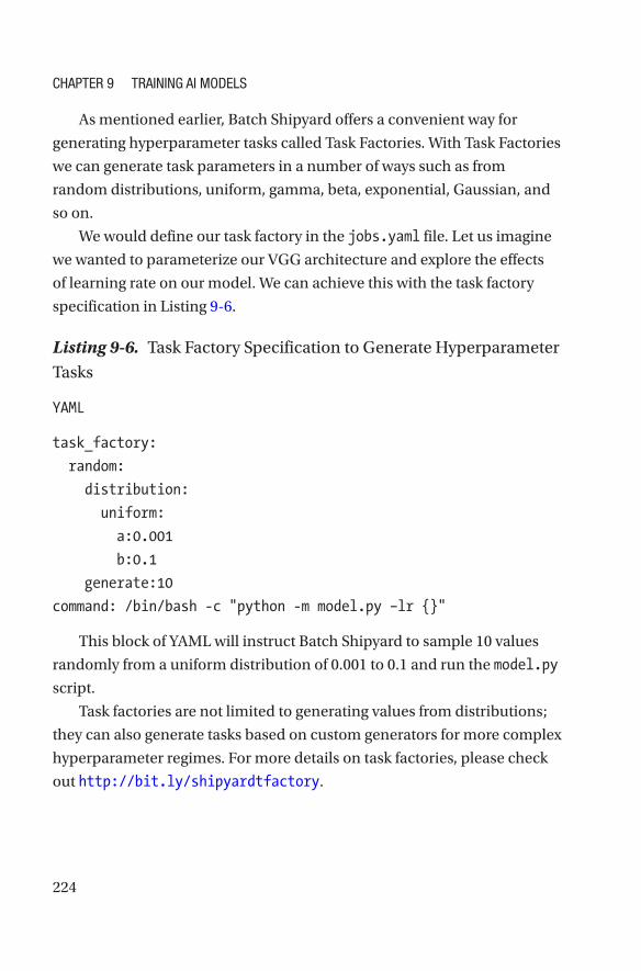
224
As mentioned earlier, Batch Shipyard offers a convenient way for
generating hyperparameter tasks called Task Factories. With Task Factories
we can generate task parameters in a number of ways such as from
random distributions, uniform, gamma, beta, exponential, Gaussian, and
so on.
We would define our task factory in the jobs.yaml file. Let us imagine
we wanted to parameterize our VGG architecture and explore the effects
of learning rate on our model. We can achieve this with the task factory
specification in Listing 9-6.
Listing 9-6. Task Factory Specification to Generate Hyperparameter
Tasks
YAML
task_factory:
random:
distribution:
uniform:
a:0.001
b:0.1
generate:10
command: /bin/bash -c "python -m model.py –lr {}"
This block of YAML will instruct Batch Shipyard to sample 10 values
randomly from a uniform distribution of 0.001 to 0.1 and run the model.py
script.
Task factories are not limited to generating values from distributions;
they can also generate tasks based on custom generators for more complex
hyperparameter regimes. For more details on task factories, please check
out http://bit.ly/shipyardtfactory.
Chapter 9 training ai Models
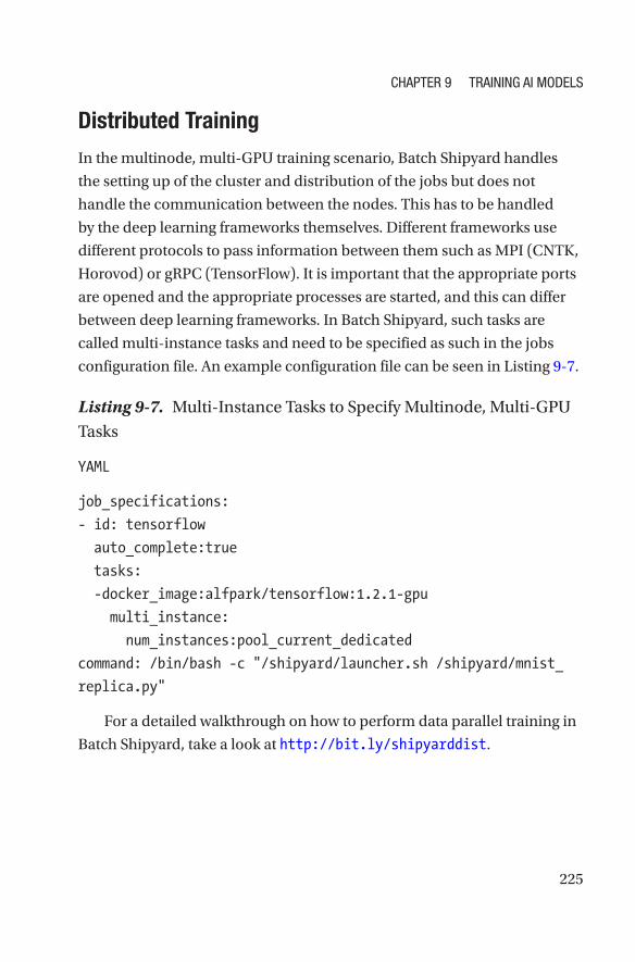
225
Distributed Training
In the multinode, multi-GPU training scenario, Batch Shipyard handles
the setting up of the cluster and distribution of the jobs but does not
handle the communication between the nodes. This has to be handled
by the deep learning frameworks themselves. Different frameworks use
different protocols to pass information between them such as MPI (CNTK,
Horovod) or gRPC (TensorFlow). It is important that the appropriate ports
are opened and the appropriate processes are started, and this can differ
between deep learning frameworks. In Batch Shipyard, such tasks are
called multi-instance tasks and need to be specified as such in the jobs
configuration file. An example configuration file can be seen in Listing 9-7.
Listing 9-7. Multi-Instance Tasks to Specify Multinode, Multi- GPU
Tasks
YAML
job_specifications:
- id: tensorflow
auto_complete:true
tasks:
-docker_image:alfpark/tensorflow:1.2.1-gpu
multi_instance:
num_instances:pool_current_dedicated
command: /bin/bash -c "/shipyard/launcher.sh /shipyard/mnist_
replica.py"
For a detailed walkthrough on how to perform data parallel training in
Batch Shipyard, take a look at http://bit.ly/shipyarddist.
Chapter 9 training ai Models

226
Training CNNs on Batch AI
Batch AI is in many ways very similar to Batch Shipyard (see Figure 9-4).
It offers a Python SDK as well as a CLI. In our example, we outline how
to use the CLI because it is slightly easier than the SDK. All of the steps
mentioned here are in the accompanying notebook, which you can use to
run the example for yourself (Chapter_09_02.ipynb).
Figure 9-4. Batch AI training steps: (1) Create the necessary Zzure resources, job configuration files, and scripts, and upload scripts to fileshare. (2) Call cluster create, which will start the process of creating our cluster. It will also pull the Docker image and make it available to the nodes in the pool and mount the fileshare. (3) Run the command specified in the job configuration. Call job stream-file to tail the output from the job. Once training is done delete the job, cluster, and Azure resources.
Batch AI uses the Azure CLI, which we installed earlier. To register for
Batch AI run the code shown in Listing 9-8.
Chapter 9 training ai Models

227
Listing 9-8. Register for Batch AI Service
BASH
az provider register -n Microsoft.BatchAI
az provider register -n Microsoft.Batch
At the time of writing, Batch AI was only available in the East US
region, so that is where we will be creating all our resources. We are
going to assume that you have already created a storage account and a
fileshare, and have uploaded the script to the fileshare. These steps are in
the accompanying notebook (Chapter_09_02.ipynb) under the sections
“Create Azure Resources” and “Define Our Model.” To create our cluster,
we run the code in Listing 9-9.
Listing 9-9. Create Batch AI Cluster
BASH
az batchai cluster create -l eastus -w workspace --name
my_cluster --vm- size STANDARD_NC6 --image UbuntuLTS --min 1
--max 1 --storage- account- name my_storage_account --storage-
account-key my_ storage_account_key --afs-name my_fileshare
--afs-mount-path azurefileshare --user-name my_username
--password my_password
All the values prefixed by my should be defined by you and wherever
they are intended to should match the Azure resources you already created.
In the preceding command, we used the az batchai cluster create
command to create a Batch AI cluster called my_cluster consisting of a
single GPU VM node. In this example, the VM runs the default Ubuntu LTS
image. If you wish to use the DSVM as the execution target, simply specify
image UbuntuDSVM instead. The VM specified is an NC6, which has one
NVIDIA K80 GPU. We also tell it to mount the fileshare at a folder named
azurefileshare. The full path of this folder on the GPU compute node is
Chapter 9 training ai Models
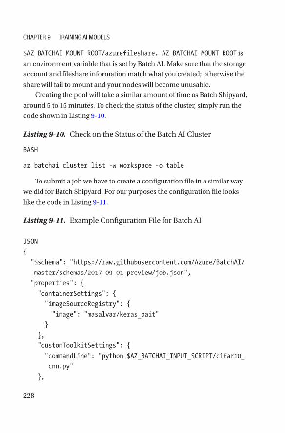
228
$AZ_BATCHAI_MOUNT_ROOT/azurefileshare. AZ_BATCHAI_MOUNT_ROOT is
an environment variable that is set by Batch AI. Make sure that the storage
account and fileshare information match what you created; otherwise the
share will fail to mount and your nodes will become unusable.
Creating the pool will take a similar amount of time as Batch Shipyard,
around 5 to 15 minutes. To check the status of the cluster, simply run the
code shown in Listing 9-10.
Listing 9-10. Check on the Status of the Batch AI Cluster
BASH
az batchai cluster list -w workspace -o table
To submit a job we have to create a configuration file in a similar way
we did for Batch Shipyard. For our purposes the configuration file looks
like the code in Listing 9-11.
Listing 9-11. Example Configuration File for Batch AI
JSON
{
" $schema": "https://raw.githubusercontent.com/Azure/BatchAI/
master/schemas/2017-09-01-preview/job.json",
"properties": {
"containerSettings": {
"imageSourceRegistry": {
"image": "masalvar/keras_bait"
}
},
"customToolkitSettings": {
" commandLine": "python $AZ_BATCHAI_INPUT_SCRIPT/cifar10_
cnn.py"
},
Chapter 9 training ai Models

229
"inputDirectories": [
{
"id": "SCRIPT",
" path": "$AZ_BATCHAI_MOUNT_ROOT/azurefileshare/cnn_example"
}
],
"nodeCount": 1,
"stdOutErrPathPrefix": "$AZ_BATCHAI_MOUNT_ROOT/azurefileshare"
}
}
For more examples, take a look at http://bit.ly/baistart. In the
jobs configuration we define our inputDirectories, what container we
want to use and the commands to execute. In the jobs definition you will
notice that under inputDirectories we defined an input directory with
the id script. This location gets mapped by Batch AI to the environment
variable AZ_BATCHAI_INPUT_SCRIPT, which we refer to in the commandLine
variable. Once we have created the job JSON file we execute the job by
running the code in Listing 9-12.
Listing 9-12. Execute the Batch AI Job
BASH
az batchai job create -w workspace -e experiment --name my_job
--cluster-name my_cluster --config job.json
We can monitor the job by running the code in Listing 9-13.
Listing 9-13. Monitor the Batch AI Job
BASH
az batchai job list -w workspace -e experiment -o table
Chapter 9 training ai Models

230
If you go to the Azure portal and click on the cluster you should see
something similar to the image in Figure 9-5. The portal also provides
other diagnostics such as the state of each job and the number of jobs in
the resource group (see Figure 9-6 and Figure 9-7). This is very convenient
for long running jobs when you simply want to check on the state of things
from any browser. The information you get from the portal with Batch AI is
richer than what you get with Batch Shipyard.
Figure 9-5. Batch AI cluster dashboard in the Azure portal
Chapter 9 training ai Models

231
To tail the output of stdout in the same way we did for Batch Shipyard,
we simply run the code in Listing 9-14.
Listing 9-14. Stream Output to Help Review Errors and Debug
Scripts with Batch AI
BASH
az batchai job file stream -w workspace -e experiment --j
my_job --output-directory-id stdouterr --f stdout.txt
Once the job is completed, to delete the job we run the code in
Listing 9-15.
Figure 9-6. Job dashboard for Batch AI
Figure 9-7. Information displayed in the portal for our resource group. Note that our cluster is called gpupool and the job keras-training-job; these are the names used in the example in the accompanying notebook.
Chapter 9 training ai Models
232
Listing 9-15. Delete Batch AI Job
BASH
az batchai job delete -w workspace -e experiment --name myjob
Now we delete the cluster with the code in Listing 9-16 so that we stop
incurring any charges for computing.
Listing 9-16. Delete Batch AI Cluster
BASH
az batchai cluster delete -w workspace -e experiment --name
mycluster
Then finally if we don’t want to keep the storage account and the
other resources we created we can clear it all up by executing the code in
Listing 9-17.
Listing 9-17. If No Longer Needed, Delete Storage Account and
Other Resources
BASH
az group delete --name myResourceGroup
Hyperparameter Tuning and Distributed Training
Hyperparameter tuning in Batch AI is not yet as simple as it is in Batch
Shipyard. There is no notion of task factories, so it requires that we create
a number of jobs where we pass different parameters to our model. In
our jobs example, therefore, the JSON file would be very similar between
our jobs, the only difference being the command, and specifically the
arguments we pass to the script. The process of hyperparameter tuning
can be made easier by using the Batch AI Python SDK rather than the
CLI. Have a look at http://bit.ly/baitsdk for further details on the
Python SDK.
Chapter 9 training ai Models
233
Distributed training is slightly easier in Batch AI than Batch Shipyard
for frameworks supported by Batch AI because Batch AI takes care
of configuring the necessary internode communication layer such as
MPI. At the time of writing, the frameworks supported are Chainer, CNTK,
TensorFlow, PyTorch, and Caffe2. For frameworks that are not supported,
it is up to the user to supply the appropriate configuration and will be the
same as Batch Shipyard. For examples on how to do this, see http://bit.
ly/bairecipes.
Variation of Batch AI with Python SDK
In the earlier example, we illustrated using Batch AI with the Azure CLI,
which is the easiest way to get started. Batch AI can also be used through
a Python SDK. The demo example described in this section can be
reproduced following the instructions given at http://bit.ly/deepbait.
In this example, rather than showcasing an example of hyperparameter
tuning or distributed training for which there are already examples, nine
different deep learning frameworks are used to train a simple CNN on
the CIFAR10 data set. In practice, being able to quickly utilize different
frameworks can be very useful because state-of-the-art implementations
of certain models might only be available in one or a small number of
frameworks. Often, though, one would select a single framework and
use that framework to do hyperparameter tuning or distributed training
as described in this chapter. However, this example also serves the
pedagogical purpose of showcasing the flexibility of the Batch AI service as
well as different ways one might interact with the service.
In this example, the project was developed and tested on an Azure
Ubuntu DLVM. Anaconda Project is used in this case to create the
environment and install dependencies, download the data, and allow
the user to interact with the project in a straightforward manner to
reproduce the demo, such as asking through a command-line prompt
for the Azure subscription identifier and name of the resource group in
Chapter 9 training ai Models
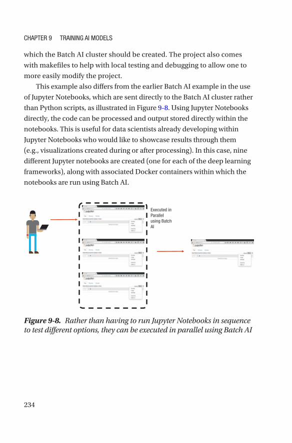
234
which the Batch AI cluster should be created. The project also comes
with makefiles to help with local testing and debugging to allow one to
more easily modify the project.
This example also differs from the earlier Batch AI example in the use
of Jupyter Notebooks, which are sent directly to the Batch AI cluster rather
than Python scripts, as illustrated in Figure 9-8. Using Jupyter Notebooks
directly, the code can be processed and output stored directly within the
notebooks. This is useful for data scientists already developing within
Jupyter Notebooks who would like to showcase results through them
(e.g., visualizations created during or after processing). In this case, nine
different Jupyter notebooks are created (one for each of the deep learning
frameworks), along with associated Docker containers within which the
notebooks are run using Batch AI.
Executed in Parallel using Batch AI
Figure 9-8. Rather than having to run Jupyter Notebooks in sequence to test different options, they can be executed in parallel using Batch AI
Chapter 9 training ai Models
235
Each of the notebooks was written to have parameters that can be
modified when they are run on the Batch AI cluster. In the example
project for illustrative purposes, the number of epochs that are run are
modified from the original file when they are run on Batch AI. Specifically,
the original notebooks that are sent to the cluster have the following
parameters in Listing 9-18 at the top of the notebook as examples.
Listing 9-18. Example Parameters at Top of Script That Are
Modified When Run by Batch AI
PYTHON
# Parameters
EPOCHS = 10
N_CLASSES=10
BATCHSIZE = 64
LR = 0.01
MOMENTUM = 0.9
GPU = True
In the job submission, the Batch AI cluster is told in this case to
modify the number of epochs to run (as just one example of a parameter
change), and the notebook is modified and run with a different number of
epochs. At the end of the run, the notebook contains a cell with all of the
parameters it was run with, as well as the output from each cell running
stored within the notebook itself. This makes it easy to look through
the results: All of the important information is stored right within the
notebook.
The steps followed to use nine different deep learning frameworks to
run a simple CNN are as follows, illustrated in Figure 9-9.
1. Create Jupyter notebooks to run on Batch AI and
transfer them to file storage.
2. Write the data to file storage.
Chapter 9 training ai Models
236
3. Create the Docker containers for each deep learning
framework and transfer them to a container registry.
4. Create a Batch AI Pool.
5. Each job will pull in the appropriate container and
notebook, and load data from the fileshare.
6. Once the job is completed the executed notebook
will be written to the fileshare.
These steps are very similar to those described before in using
Batch AI with the CLI, only with Jupyter Notebooks. Besides the parallel
processing ability that allows for a reduction in the experimentation time
enabled through Batch AI, this scenario also illustrates the power of cloud
computing in that many machines can be spun up on demand, used for
the processing they are needed for, and then the cluster can be shut down.
This provides the data scientist more flexibility at a large reduction in cost,
with no special hardware to procure or systems to manage.
Chapter 9 training ai Models

237
A number of helper functions are included to make interaction with
the Batch AI cluster easy, such as the setup_cluster( ) function shown in
Figure 9-10 and print_jobs_summary( ) as shown in Figure 9-11.
IAI
1
2
3
Batch AI Pool 45
6
Figure 9-9. Steps required to run a simple CNN using nine different deep learning frameworks for illustration purposes of the flexibility of Batch AI, with code processed and output stored within Jupyter Notebooks.
Chapter 9 training ai Models
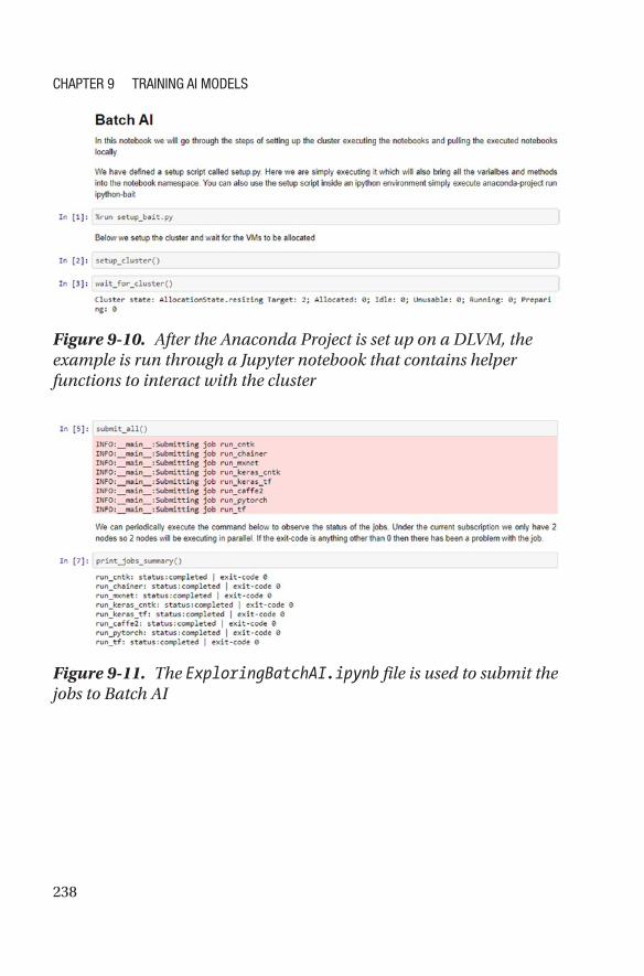
238
Figure 9-11. The ExploringBatchAI.ipynb file is used to submit the jobs to Batch AI
Figure 9-10. After the Anaconda Project is set up on a DLVM, the example is run through a Jupyter notebook that contains helper functions to interact with the cluster
Chapter 9 training ai Models
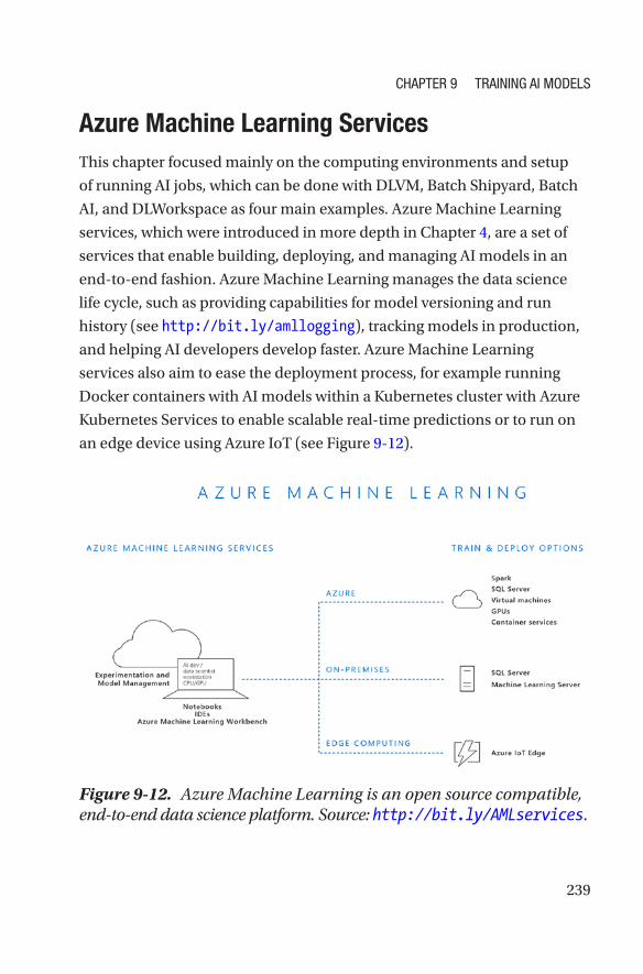
239
Azure Machine Learning ServicesThis chapter focused mainly on the computing environments and setup
of running AI jobs, which can be done with DLVM, Batch Shipyard, Batch
AI, and DLWorkspace as four main examples. Azure Machine Learning
services, which were introduced in more depth in Chapter 4, are a set of
services that enable building, deploying, and managing AI models in an
end-to-end fashion. Azure Machine Learning manages the data science
life cycle, such as providing capabilities for model versioning and run
history (see http://bit.ly/amllogging), tracking models in production,
and helping AI developers develop faster. Azure Machine Learning
services also aim to ease the deployment process, for example running
Docker containers with AI models within a Kubernetes cluster with Azure
Kubernetes Services to enable scalable real-time predictions or to run on
an edge device using Azure IoT (see Figure 9-12).
Figure 9-12. Azure Machine Learning is an open source compatible, end-to-end data science platform. Source: http://bit.ly/AMLservices.
Chapter 9 training ai Models
240
Some of the services mentioned in this chapter, such as the DLVM and
Batch AI, can be set up as the computing context within an Azure Machine
Learning project. As of this writing, Azure Machine Learning services
works with Python and is available in several Azure regions. In addition,
there are AI extensions for Visual Studio and Visual Studio Code that allow
interacting with the Azure Machine Learning platform (see http://bit.
ly/aivisstdio). As the service is updating frequently, we focused on the
core computing environments in this chapter and suggest reading the
current documentation on Azure Machine Learning services available at
http://bit.ly/AMLservices.
Other Options for AI Training on AzureThere are numerous other options for AI training on Azure that we do not
describe in depth, but some of which we mention briefly here. The first
example builds on Apache Spark, which is a popular general-purpose engine
for big data processing. There are several offerings of Apache Spark on Azure
such as Azure Databricks and Azure HDInsight. One popular option for
training AI models with Spark is through the use of the MMLSpark library by
Microsoft, which provides a number of deep learning and data science tools,
available as open source on Github at http://bit.ly/mmlSpark. MMLSpark
integrates Spark ML pipelines with the deep learning framework CNTK as
well as OpenCV. This is especially useful if the data for an AI solution already
reside in SPARK. MMLSpark can be used to train deep learning models on
GPU nodes and can thus be used on a DLVM attached to the HDInsight
Spark cluster as described at http://bit.ly/MMLSparkGPU.
Another alternative to attaching a GPU VM to a Spark cluster is utilizing
transfer learning to apply a pretrained model using MMLSpark in a parallel
fashion on a Spark cluster and then train a classifier using one of the many
ML packages in Spark. This was used for snow leopard conservation to
predict images containing snow leopards and assist conservation efforts as
described in a blog post by Hamilton, Sengupta, and Astala (2017).
Chapter 9 training ai Models

241
AI training can also be scaled out through the use of a cluster of
Docker containers such as through the use of Kubernetes. Although we
have seen the use of Kubernetes clusters mainly for the deployment and
hosting of AI models to date, it is also possible to use them for large-scale
training. Zhang and Buchwalter (2017) described how they used Azure
Container Services Engine (ACS-engine) that generates Azure Resource
Manager templates that are needed to deploy the cluster with everything
configured. In their case working alongside the startup Litbit, a Kubernetes
cluster was used to scale different types of VM pools (CPU, GPUs) up and
down based on the demand of the given workload. Tok (2017) gave an
overview of using CNTK with Kubernetes through ACS-engine along with
a detailed walkthrough of how to set up the cluster, for both training and
deploying deep learning models at scale.
SummaryThis chapter presented various options you can use to train your AI model.
If you simply want to experiment, then the DLVM is probably the best
choice because it is the quickest and easiest to set up. If you are looking
to run hyperparameter tuning, distributed training, or model training as
part of an automated pipeline, then Batch AI or Batch Shipyard will be the
best tools for the job. DLWorkspace is also a good choice for large-scale
experimentation, but today we would mostly recommend it only if the
other two options are not suitable. The cluster-based method of training
might seem daunting at first, but it quickly confers benefits. Batch AI is the
easiest to use and set up and Batch Shipyard is the most feature rich. We
have only scratched the surface of what is possible with these powerful
tools. For detailed documentation, check out http://bit.ly/azbai,
http://bit.ly/azshipyard, and http://bit.ly/azdlwork. In the next
chapter, we give an overview of different options for deploying trained
deep learning models so they can be used within AI applications.
Chapter 9 training ai Models
243© Mathew Salvaris, Danielle Dean, Wee Hyong Tok 2018 M. Salvaris et al., Deep Learning with Azure, https://doi.org/10.1007/978-1-4842-3679-6_10
CHAPTER 10
Operationalizing AI ModelsThe previous chapter covered what constitutes an AI model, the different
types of models we can create, and how to train and build these models.
An AI model does not become useful until it is deployed somewhere and
consumed by the end user. This chapter describes the various options
available on Azure to deploy your models. We provide general guidelines
on what to use and when, but this is by no means an exhaustive guide to
the Azure platform. In the following sections we discuss the metrics over
which we compare the various deployment platforms. Then we discuss
the platforms we have found to be suitable for deploying ML models
and highlight their pros and cons. We also present simple use cases
and architectures for each of them so that you get an idea of how they
would fit into a larger solution. We also provide a step-by-step tutorial for
deployment of a CNN to Azure Kubernetes Services (AKS) with GPU nodes
as a hands-on guide for one recommended option for building a real-time
request–response AI system.
Operationalization PlatformsA common dichotomy when looking at operationalization of a model is
whether the scoring requests will be batch or real time. An example of
a batch workload is when we have large number of records given to us
244
infrequently such as every 24 hours, that need to be scored. These records
could be images or other types of data. A real-time workload is when
the service must always be up and receives a small number of records to
score relatively frequently. An example might be a phone app that sends
a picture to determine what type of animal is in the picture. The examples
provided fit quite nicely into their respective classifications, but in reality
things are often a lot less discrete. For example, we might have a real-time
workload that requires massive amounts of computing or other constraints
on our solution that break key architecture assumptions. That is why it
is often better to think about these solutions belonging to a continuum
where each solution can be partially stretched beyond what it is ideally
suited for.
A key consideration when deploying models is dependency and
environment management. This is not a problem unique to AI models: It is
common for all types of deployed applications, but it becomes especially
acute for AI applications due to their often complicated dependencies
and hardware requirements. For this reason, services that use Docker
containers are often preferred because this makes it easy to keep the
same environment for development and test as well as ensure that all
dependencies are satisfied. If you are new to Docker, we recommend the
basic overview at http://bit.ly/DockerDS.
As we mentioned earlier, AI models also have hardware requirements;
these are often less demanding than the training environments but
depending on the scenario might still require a reasonable amount
of computing resources. That is why another consideration for the
deployment options is the hardware available on the platform and
specifically the availability of GPUs. Without the GPUs the throughput
could be quite limited, meaning that the service will either have to deal
with slow responses or have to scale out the compute.
Chapter 10 OperatiOnalizing ai MOdels
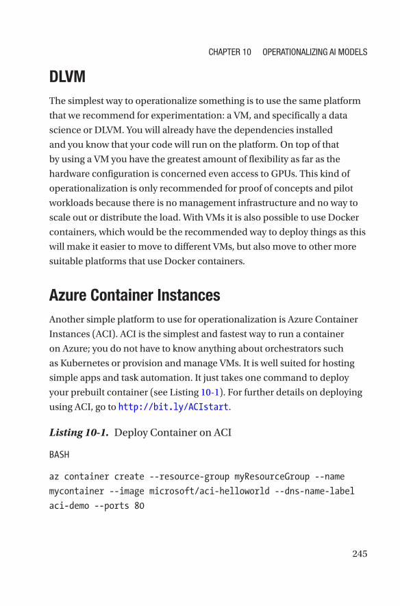
245
DLVMThe simplest way to operationalize something is to use the same platform
that we recommend for experimentation: a VM, and specifically a data
science or DLVM. You will already have the dependencies installed
and you know that your code will run on the platform. On top of that
by using a VM you have the greatest amount of flexibility as far as the
hardware configuration is concerned even access to GPUs. This kind of
operationalization is only recommended for proof of concepts and pilot
workloads because there is no management infrastructure and no way to
scale out or distribute the load. With VMs it is also possible to use Docker
containers, which would be the recommended way to deploy things as this
will make it easier to move to different VMs, but also move to other more
suitable platforms that use Docker containers.
Azure Container InstancesAnother simple platform to use for operationalization is Azure Container
Instances (ACI). ACI is the simplest and fastest way to run a container
on Azure; you do not have to know anything about orchestrators such
as Kubernetes or provision and manage VMs. It is well suited for hosting
simple apps and task automation. It just takes one command to deploy
your prebuilt container (see Listing 10-1). For further details on deploying
using ACI, go to http://bit.ly/ACIstart.
Listing 10-1. Deploy Container on ACI
BASH
az container create --resource-group myResourceGroup --name
mycontainer --image microsoft/aci-helloworld --dns-name-label
aci-demo --ports 80
Chapter 10 OperatiOnalizing ai MOdels
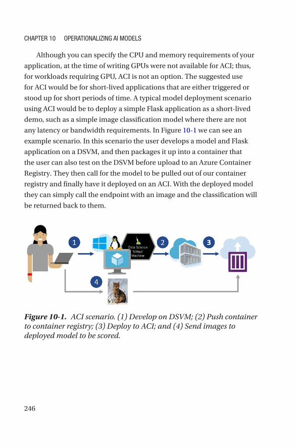
246
Although you can specify the CPU and memory requirements of your
application, at the time of writing GPUs were not available for ACI; thus,
for workloads requiring GPU, ACI is not an option. The suggested use
for ACI would be for short-lived applications that are either triggered or
stood up for short periods of time. A typical model deployment scenario
using ACI would be to deploy a simple Flask application as a short-lived
demo, such as a simple image classification model where there are not
any latency or bandwidth requirements. In Figure 10-1 we can see an
example scenario. In this scenario the user develops a model and Flask
application on a DSVM, and then packages it up into a container that
the user can also test on the DSVM before upload to an Azure Container
Registry. They then call for the model to be pulled out of our container
registry and finally have it deployed on an ACI. With the deployed model
they can simply call the endpoint with an image and the classification will
be returned back to them.
Figure 10-1. ACI scenario. (1) Develop on DSVM; (2) Push container to container registry; (3) Deploy to ACI; and (4) Send images to deployed model to be scored.
Chapter 10 OperatiOnalizing ai MOdels
247
Azure Web AppsAzure Web Apps is another quick and easy way of deploying models. They
can either be standard Web Apps that are Windows based or Linux Web
Apps. Both support a number of programming languages and Linux Web
Apps support Docker containers. The use case for Azure Web Apps is the
same as ACI. They can be a little harder to set up and configure, but they
are also cheaper for longer running deployments. The web apps also offer
nice features such as deploying from a git repository as well as a CLI to
install packages. For further information on web apps, see http://bit.ly/
AzureWebApps.
Azure Kubernetes ServicesAKS is a managed Kubernetes cluster configuration. It is like a standard
Kubernetes cluster except that the management of the master nodes
is handled by Azure. This translates to reduced overhead and cost
because you only have to pay for the compute of the agent nodes. It uses
Kubernetes, which is a popular open source Docker orchestrator, so it is
easy to navigate for those familiar with Kubernetes and because it is an
open source project there is lots of information from which to draw.
AKS recently enabled deployment to GPU VMs, opening the possibility
to run GPU AI models on it. In fact, AKS is our recommended way to
deploy real-time workloads. A typical scenario for AKS would be where
we need to set up a real-time service that needs to scale with demand and
also be fault tolerant. Because we can use any size (SKU) of VM including
GPUs this is the ideal solution for demanding applications. The setup and
management is considerably more involved than what was shown for the
ACI. An example of how to deploy things on an orchestrated container
cluster can be found at http://bit.ly/ACSTutorial. This uses the older
Azure Container Services service, so some of the commands will differ.
Chapter 10 OperatiOnalizing ai MOdels

248
The scenario is very similar to the one explained for ACI deployment
except that we also have a load balancer so that when a request is made
the load can be distributed appropriately between the deployed pods (see
Figure 10-2). The creation of the container is omitted from the diagram
but would be identical to what is shown in Figure 10-1. Using AKS we can
also set up autoscaling rules so that the number of pods and nodes in our
cluster can change based on demand.
Figure 10-2. AKS scenario: (1) Develop on DSVM, (2) Push container to container registry, (3) Deploy to AKS, and (4) Send images to service, which get balanced across the pods using load balancer.
To deploy an AI model on AKS you need the following:
1. Your model and an API to call it.
2. The Flask web application that will handle the requests.
3. A Docker container that contains the model, Flask
application, and necessary dependencies.
Once you have these you can create the cluster with the command
shown in Listing 10-2. The command will create a cluster called
myGPUCluster with one node that is an NC6 VM. An NC6 VM has a
single K80 GPU that will speed up the inference of our deep learning
Chapter 10 OperatiOnalizing ai MOdels
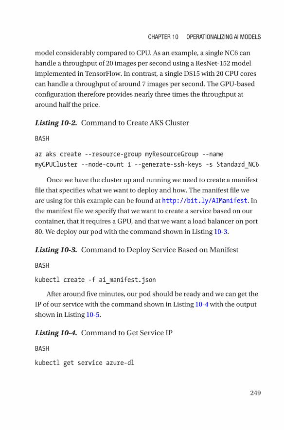
249
model considerably compared to CPU. As an example, a single NC6 can
handle a throughput of 20 images per second using a ResNet-152 model
implemented in TensorFlow. In contrast, a single DS15 with 20 CPU cores
can handle a throughput of around 7 images per second. The GPU- based
configuration therefore provides nearly three times the throughput at
around half the price.
Listing 10-2. Command to Create AKS Cluster
BASH
az aks create --resource-group myResourceGroup --name
myGPUCluster --node-count 1 --generate-ssh-keys -s Standard_NC6
Once we have the cluster up and running we need to create a manifest
file that specifies what we want to deploy and how. The manifest file we
are using for this example can be found at http://bit.ly/AIManifest. In
the manifest file we specify that we want to create a service based on our
container, that it requires a GPU, and that we want a load balancer on port
80. We deploy our pod with the command shown in Listing 10-3.
Listing 10-3. Command to Deploy Service Based on Manifest
BASH
kubectl create -f ai_manifest.json
After around five minutes, our pod should be ready and we can get the
IP of our service with the command shown in Listing 10-4 with the output
shown in Listing 10-5.
Listing 10-4. Command to Get Service IP
BASH
kubectl get service azure-dl
Chapter 10 OperatiOnalizing ai MOdels
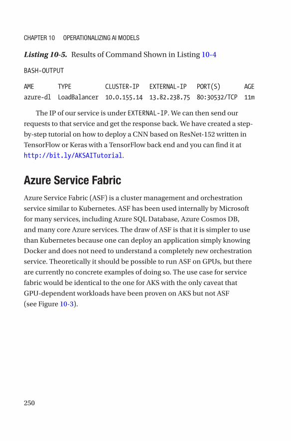
250
Listing 10-5. Results of Command Shown in Listing 10-4
BASH-OUTPUT
AME TYPE CLUSTER-IP EXTERNAL-IP PORT(S) AGE
azure-dl LoadBalancer 10.0.155.14 13.82.238.75 80:30532/TCP 11m
The IP of our service is under EXTERNAL-IP. We can then send our
requests to that service and get the response back. We have created a step-
by- step tutorial on how to deploy a CNN based on ResNet-152 written in
TensorFlow or Keras with a TensorFlow back end and you can find it at
http://bit.ly/AKSAITutorial.
Azure Service FabricAzure Service Fabric (ASF) is a cluster management and orchestration
service similar to Kubernetes. ASF has been used internally by Microsoft
for many services, including Azure SQL Database, Azure Cosmos DB,
and many core Azure services. The draw of ASF is that it is simpler to use
than Kubernetes because one can deploy an application simply knowing
Docker and does not need to understand a completely new orchestration
service. Theoretically it should be possible to run ASF on GPUs, but there
are currently no concrete examples of doing so. The use case for service
fabric would be identical to the one for AKS with the only caveat that
GPU-dependent workloads have been proven on AKS but not ASF
(see Figure 10-3).
Chapter 10 OperatiOnalizing ai MOdels

251
Batch AIIn Chapter 9, we discussed Batch AI, and all the benefits we mentioned
previously in terms of flexibility of compute and scalability transfer to
operationalization as well. Batch AI is most suited to massively parallel batch
scenarios where the cluster can be quickly spun up, the job executed in
parallel, and then spun down. Because Batch AI itself does not cost anything,
you only need to pay for the compute you use, making it an extremely
efficient solution. A scenario for using Batch AI is shown in Figure 10-4.
We assume you have already trained the model and have wrapped it in an
appropriate API and Docker container and pushed it all to an ACR. The user
uploads one or more videos to be processed by our deep learning model. An
Azure function receives the notification that data have been uploaded to a
blob and spins up the Batch AI cluster. Meanwhile, another Azure function
reads the videos and queues them up in an Azure Service Bus. As the cluster
comes online it pulls in the appropriate container and spins it up. The
application in the container subscribes to the appropriate topic and sees
what jobs are available. Each VM now will independently pull a message
Figure 10-3. Service Fabric scenario: (1) Develop on DSVM, (2) Push container to container registry, (3) Deploy container to Service Fabric, and (4) Send images to the service to be scored.
Chapter 10 OperatiOnalizing ai MOdels
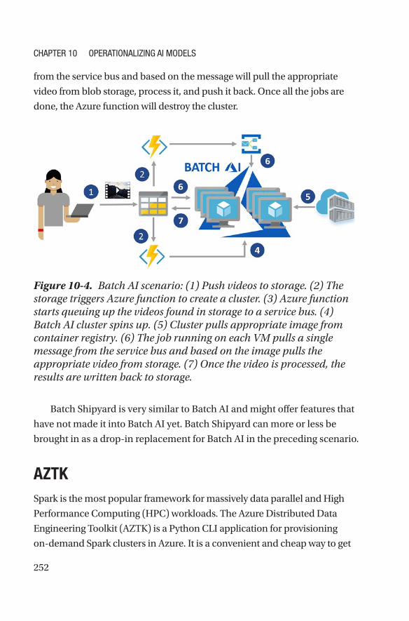
252
from the service bus and based on the message will pull the appropriate
video from blob storage, process it, and push it back. Once all the jobs are
done, the Azure function will destroy the cluster.
Figure 10-4. Batch AI scenario: (1) Push videos to storage. (2) The storage triggers Azure function to create a cluster. (3) Azure function starts queuing up the videos found in storage to a service bus. (4) Batch AI cluster spins up. (5) Cluster pulls appropriate image from container registry. (6) The job running on each VM pulls a single message from the service bus and based on the image pulls the appropriate video from storage. (7) Once the video is processed, the results are written back to storage.
Batch Shipyard is very similar to Batch AI and might offer features that
have not made it into Batch AI yet. Batch Shipyard can more or less be
brought in as a drop-in replacement for Batch AI in the preceding scenario.
AZTKSpark is the most popular framework for massively data parallel and High
Performance Computing (HPC) workloads. The Azure Distributed Data
Engineering Toolkit (AZTK) is a Python CLI application for provisioning
on-demand Spark clusters in Azure. It is a convenient and cheap way to get
Chapter 10 OperatiOnalizing ai MOdels
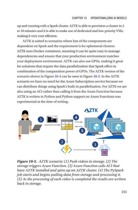
253
up and running with a Spark cluster. AZTK is able to provision a cluster in 5
to 10 minutes and it is able to make use of dedicated and low-priority VMs,
making it very cost- efficient.
AZTK is suited to scenarios where lots of the components are
dependent on Spark and the requirement is for ephemeral clusters.
AZTK uses Docker containers, meaning it can be quite easy to manage
dependencies and ensure that your production environment matches
your deployment environment. AZTK can also use GPUs, making it great
for solutions that require the data parallelization that Spark offers in
combination of the computation power of GPUs. The AZTK version of the
scenario shown in Figure 10-4 can be seen in Figure 10-5. In the AZTK
scenario we have no need for the Azure Subscription service because we
can distribute things using Spark’s built-in parallelization. For AZTK we are
also using an ACI rather than calling it from the Azure Function because
AZTK is written in Python and Python support on Azure Functions was
experimental at the time of writing.
Figure 10-5. AZTK scenario: (1) Push videos to storage. (2) The storage triggers Azure Function. (3) Azure Function calls ACI that have AZTK installed and spins up an AZTK cluster. (4) The PySpark job starts and begins pulling data from storage and processing it. (5) As the processing of each video is completed the results are written back to storage.
Chapter 10 OperatiOnalizing ai MOdels
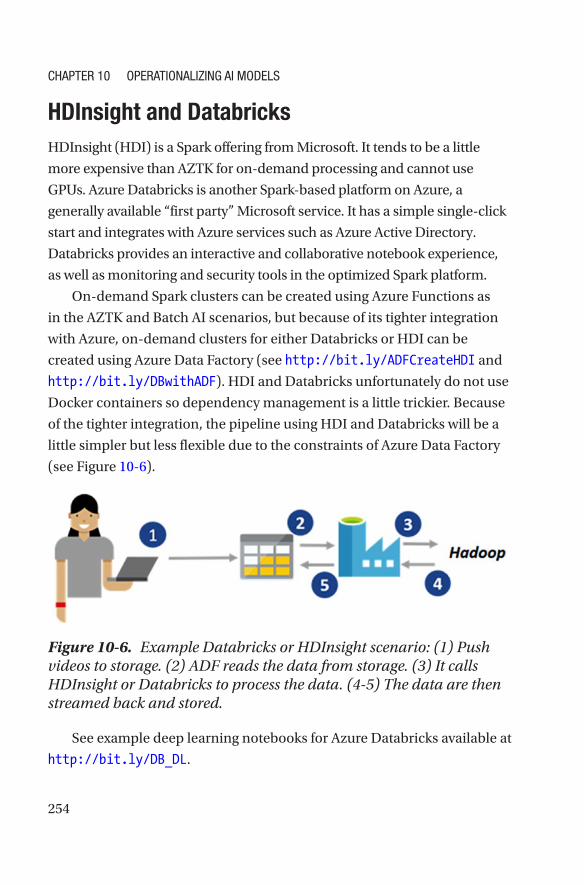
254
HDInsight and DatabricksHDInsight (HDI) is a Spark offering from Microsoft. It tends to be a little
more expensive than AZTK for on-demand processing and cannot use
GPUs. Azure Databricks is another Spark-based platform on Azure, a
generally available “first party” Microsoft service. It has a simple single- click
start and integrates with Azure services such as Azure Active Directory.
Databricks provides an interactive and collaborative notebook experience,
as well as monitoring and security tools in the optimized Spark platform.
On-demand Spark clusters can be created using Azure Functions as
in the AZTK and Batch AI scenarios, but because of its tighter integration
with Azure, on-demand clusters for either Databricks or HDI can be
created using Azure Data Factory (see http://bit.ly/ADFCreateHDI and
http://bit.ly/DBwithADF). HDI and Databricks unfortunately do not use
Docker containers so dependency management is a little trickier. Because
of the tighter integration, the pipeline using HDI and Databricks will be a
little simpler but less flexible due to the constraints of Azure Data Factory
(see Figure 10-6).
Figure 10-6. Example Databricks or HDInsight scenario: (1) Push videos to storage. (2) ADF reads the data from storage. (3) It calls HDInsight or Databricks to process the data. (4-5) The data are then streamed back and stored.
See example deep learning notebooks for Azure Databricks available at
http://bit.ly/DB_DL.
Chapter 10 OperatiOnalizing ai MOdels
255
SQL ServerTo perform computig close to where the data are, SQL Server is a great
option for deployment when data are already stored in SQL. The ideal
scenario for such a deployment would be that SQL Server is already being
used or the scenario would benefit from having the model execute as close
to the data as possible. The data proximity requirement is usually the result
of two things, data gravity and data sensitivity. Data gravity refers to the fact
that large volumes of data cause a “gravitational pull” on the computation
due to the costs of moving the data around. Data sensitivity refers to privacy
and security concerns when having data cross different systems and the
possibility of data being left behind or the security weakened due to the
multiple data transfers. SQL Server is very flexible, as it can be installed on
Windows and Linux and can be deployed on VMs with GPU to accelerate
deep learning scenarios (see http://bit.ly/SQLServerDeepL). Both
Python and R integration are available for SQL Server so data scientists can
use whatever language they are most comfortable with. More examples on
deploying models on SQL Server can be found at http://bit.ly/SQLML.
Operationalization OverviewWe have presented a number of operationalization platforms and it can be
hard to choose among them. As we mentioned earlier it is good to think
about these services belonging on a continuum that ranges from strictly
batch to real time, with services like Batch AI and AZTK belonging to
the batch end of the spectrum and services like AKS and ASF belonging
to the real-time end of the spectrum. In Figure 10-7 you can see a visual
representation of this continuum: On the left are the more batch-like
platforms and on the right the more real-time platforms. Figure 10-7 does
not imply that the leftmost or rightmost options are the recommended
approaches for batch and real-time processing, respectively, only that
these platforms are most appropriate for that type of processing.
Chapter 10 OperatiOnalizing ai MOdels

256
Figure 10-7. Batch to real-time continuum
Figure 10-7 is just a general guideline, as it is possible to use these
options in many ways. For example, even though Spark on HDI or Azure
Databricks are typically associated with batch workloads, there are
options for creating real-time workloads, enabled, for example, through
MMLSpark Serving as described at http://bit.ly/MMLSparkStreaming.
You will have also gleaned from the sections on each of the services
that each have strengths and weaknesses. In Figure 10-8 you can see a
visual representation of the attributes of each of the services. The services
are listed on the left side of the heatmap and the metrics along the top.
Each service receives a rating indicated by the color of the box that is based
on the color bar on right side of the heatmap. We compare the service
across five metrics: speed, scalability, data proximity, debug environment,
and ease of deployment.
Chapter 10 OperatiOnalizing ai MOdels

257
Speed refers to the hardware available to each of the services; for AI
models this mainly revolves around whether GPUs are available for it
or not. Scalability refers to whether the service can be easily scaled up
and out. Data proximity refers to how close the compute is to the data;
this is mainly a consideration when we don’t want to move the data due
to either volume or security reasons. Debug environment refers to how
easy it is to develop for the platform; the main consideration across this
axis is whether the service uses Docker containers or not. Finally, ease of
deployment refers to how easy it is to deploy the model and whether there
is a steep learning curve to get things working.
Although there are many nuances and reasons to deviate from this
recommendation, for real-time processing of deep learning models, we
recommend AKS using GPU nodes. As mentioned earlier, we have created a
step-by-step tutorial on how to deploy a CNN based on ResNet-152 written
in TensorFlow or Keras with a TensorFlow back end, and you can find it
at http://bit.ly/AKSAITutorial. For batch processing of deep learning
models, at the time of this writing we recommend using Batch AI. An
example using TensorFlow can be found at http://bit.ly/BatchAIEx.
Figure 10-8. Heatmap of deployment services
Chapter 10 OperatiOnalizing ai MOdels
258
We focused primarily here on operationalizing deep learning models
on Azure. Deep learning models can also be trained on the cloud and then
operationalized in different environments, such as IoT edge as discussed
in the next section, as well as natively on Windows devices through ONNX
as described at http://bit.ly/WindowsONNX.
Azure Machine Learning ServicesThe preceding example to deploy an AI model to AKS can be a little
daunting, especially to those not familiar with Docker. To this end, AML
offers options that make operationalization of AI models easier: You
simply supply the model file, your dependencies in a YAML file, and finally
the model driver file, and it will create the appropriate Docker container
and deploy it to AKS (see http://bit.ly/amldeploy). It offers easy and
convenient ways to test your deployment locally as well as scale the service
as needed. See the blog post by Zhu, Iordanescu, and Karmanov (2018) as
an example of using Azure Machine Learning to deploy a deep learning
model for detecting diseases from chest x-ray images. Azure Machine
Learning also assists in the deployment of deep learning models to IoT
edge devices as described at http://bit.ly/DLtoIOT.
In previous chapters we mentioned the usefulness of transfer learning
and in this chapter we also highlighted the benefits of using GPUs for
inference. AML services now offers the ability to use a pretrained ResNet
50 model on FPGAs for inference. FPGAs offer a considerable speed
increase over CPUs and GPUs at a very low cost. Benchmarking showed
that a single FPGA could score around 500 images per second and cost less
than 0.2 cents to score 10,000 images. To use this service simply follow the
instructions given at http://bit.ly/msfpga. It has a number of Jupyter
Notebooks that go through how to train your model based on the features,
but also how to deploy and test the model.
Chapter 10 OperatiOnalizing ai MOdels
259
SummaryThis chapter covered a number of operationalization options offered
on Azure. It went through the options of deploying models using simple
managed services such as ACI and Azure Web Apps to more complicated
setups with GPU support such as AKS and Batch AI. We also covered
both request–response scenarios as well as batch scenarios. We gave a
comparative overview of what we believe the strengths and weaknesses
of each of the services offered are. With this guidance you should be able
to choose the most appropriate option for your scenario and deploy your
model to make your model available within a production AI solution.
Chapter 10 OperatiOnalizing ai MOdels
261© Mathew Salvaris, Danielle Dean, Wee Hyong Tok 2018 M. Salvaris et al., Deep Learning with Azure, https://doi.org/10.1007/978-1-4842-3679-6
APPENDIX
Notes Chapter 1AI Index. (2017). AI Index 2017 annual report. Retrieved from http://cdn.
aiindex.org/2017-report.pdf
Bengio, Y. (2010). Very brief introduction to machine learning for AI.
Retrieved from http://www.iro.umontreal.ca/~pift6266/H10/notes/
mlintro.html
Bing. (2017, December 13). Bing launches new intelligent search
features, powered by AI. Retrieved from https://blogs.bing.com/
search/2017-12/search-2017-12-December-AI-Update
Brynjolfsson, E., & Mitchell, T. (2017). What can machine learning do?
Workforce implications. Science, 358(6370), 1530–1534.
Bunting, P. (2017). Using big data, the cloud, and AI to enable
intelligence at scale. Microsoft Ignite. Retrieved from https://myignite.
microsoft.com/videos/55333
Dahl, G. E., Yu, D., Deng, L., & Acero, A. (2011). Context-dependent
pre-trained deep neural networks for large-vocabulary speech recognition.
IEEE Transactions on Audio, Speech, and Language Processing, 20(1), 30–42.
Gershgorn, D. (2017, July 26). The data that transformed AI research—
and possibly the world. Quartz. Retrieved from https://qz.com/1034972/
the-data-that-changed-the-direction-of-ai-research-and-
possibly-the-world/
262
Goldberg, Y. (2016). A primer on neural network models for natural
language processing. Journal of Artifical Intelligence Research, 57, 345–420.
Retrieved from https://www.jair.org/media/4992/live-4992-9623-
jair.pdf
Goodfellow, I., Bengio, Y., & Courville, A. (2016). Deep learning.
Cambridge, MA: MIT Press.
He, K., Zhang, X., Ren, S., & Sun, J. (2015, June). Deep residual learning
for image recognition. Paper presented at the IEEE Conference on
Computer Vision and Pattern Recognition, Las Vegas, NV. Retrieved from
arXiv:1512.03385
Jia, R., & Liang, P. (2017). Adversarial examples for evaluating reading
comprehension systems. EMNLP. Retrieved from https://arxiv.org/
abs/1707.07328
Linn, A. (2017, December 13). People want more intelligent technology
tools: AI is helping with that. Retrieved from https://news.microsoft.
com/features/people-want-more-intelligent-technology-tools-ai-
is-helping-with-that/?lipi=urn%3Ali%3Apage%3Ad_flagship3_pulse_
read%3B2NMDyj2gQIecJUBYgBAbWg%3D%3D
Linn, A. (2018, January 15). Microsoft creates AI that can read a
document and answer questions about it as well as a person. Retrieved from
https://blogs.microsoft.com/ai/microsoft-creates-ai-can-read-
document-answer-questions-well-person/
Marr, B. (2016, December 6). What is the difference between
artificial intelligence and machine learning? Forbes. Retrieved from
https://www.forbes.com/sites/bernardmarr/2016/12/06/what-is-
the-difference-between-artificial-intelligence-and-machine-
learning/#6c9613e82742
Merity, S. (2016, July). In deep learning, architecture engineering is the
new feature engineering. Retrieved from https://www.kdnuggets.com/
2016/07/deep-learning-architecture-engineering-feature-
engineering.html
Appendix notes
263
Microsoft. (2015, July 26). Fueling the oil and gas industry with IoT.
Retrieved from https://customers.microsoft.com/en-us/story/
fueling-the-oil-and-gas-industry-with-iot-1
Microsoft Customer Stories. (2017, February 6). Starship Commander:
Virtual reality meets Cognitive Services in new science-fiction game.
Retrieved from https://customers.microsoft.com/en-us/story/human-
interact-cognitive-services
Microsoft Form 10-K. (2017, June). U.S. Securities and Exchange
Commission. Retrieved from https://www.sec.gov/Archives/edgar/
data/789019/000156459017014900/msft-10k_20170630.htm
Microsoft News. (2017, June). Democratizing AI: For every person
and every organization. Retrieved from https://news.microsoft.com/
features/democratizing-ai/
Microsoft Translator. (2017, December). Presentation Translator, a
Microsoft Garage project. Retrieved from https://translator.microsoft.
com/help/presentation-translator/
Nadella, S. (2016, June). The partnership of the future: Microsoft’s CEO
explores how humans and A.I. can work together to solve society’s greatest
challenges. Slate. Retrieved from http://www.slate.com/articles/
technology/future_tense/2016/06/microsoft_ceo_satya_nadella_
humans_and_a_i_can_work_together_to_solve_society.html
Nadella, S. (2017). Hit refresh: The quest to rediscover Microsoft’s soul
and imagine a better future for everyone. New York, NY: HarperCollins.
Nehme, R. (2016, November 2). Connected drones: 3 powerful lessons
we can all take away. Retrieved from https://blogs.technet.microsoft.
com/machinelearning/2016/11/02/connected-drones-3-powerful-
lessons-we-can-all-take-away/
Rajpurkar, P., Zhang, J., Lopyrev, K., & Liang, P. (2016). SQuAD:
100,000+ questions for machine comprehension of text. Retrieved from
https://arxiv.org/abs/1606.05250
Appendix notes
264
Russakovsky, O., Deng, J., Su, H., Krause, J., Satheesh, S., Ma, S.,
Huang, Z., Karpathy, A., Khosla, A., Bernstein, M., & Berg, A.C. (2015).
Imagenet large scale visual recognition challenge. International Journal of
Computer Vision, 115(3), 211–252.
Silver, D., Huang, A., Maddison, C., Guez, A., Sifre, L., van den
Driessche, G., et al. (2016). Mastering the game of Go with deep neural
networks and tree search. Nature, 529, 484–489.
van Seijen, H. (2017, December 6). Hybrid reward architecture
and the fall of Ms. Pac-Man with Dr. Harm van Seijen. Retrieved from
https://www.microsoft.com/en-us/research/blog/hybrid-reward-
architecture-fall-ms-pac-man-dr-harm-van-seijen/
Xiong, W., Droppo, J., Huang, X., Seide, F., Seltzer, M., Stolcke, A.,
et al. (2016). Achieving human parity in conversational speech recognition
(Technical Report MSR-TR-2016-71). Retrieved from https://arxiv.org/
pdf/1610.05256.pdf
Chapter 2Esteva, A., Kuprel, B., Novoa, R., Ko, J., Swetter, S., Blau, H., & Thrun, S.
(2017). Dermatologist-level classification of skin cancer with deep neural
networks. Nature, 542, 115–118.
Goodfellow, I., Pouget-Abadie, J., Mirza, M., Xu, B., Warde-Farley, D.,
Ozair, S., et al. (2014). Generative adversarial nets. Retrieved from
arXiv:1406.2661v1
Kuchaiev, O., & Ginsburg, B. (2017, August). Training deep
autoencoders for collaborative filtering. Retrieved from https://arxiv.
org/abs/1708.01715
Metz, C., & Collins, K. (2018, January 2). How an A.I. “cat-and-mouse
game.” New York Times. Retrieved from https://www.nytimes.com/
interactive/2018/01/02/technology/ai-generated-photos.html
Appendix notes
265
Rajpurkar, P., Hannun, A., Haghpanahi, M., Bourn, C., & Ng, A.
(2017). Cardiologist-level arrhythmia detection with convolutional neural
networks. Retrieved from arXiv:1707.01836v1
Chapter 3Abdi, M., & Nahavandi, S. (2017, March). Multi-residual metworks:
Improving the speed and accuracy of residual networks. Retrieved from
https://arxiv.org/abs/1609.05672v4
Bergstra, J., Yamins, D., & Cox, D.D. (2013, June). Making a science of
model search: Hyperpa-rameter optimization in hundreds of dimensions for
vision architectures. ICML, Atlanta.
Bolukbasi, T., Chang, K., Zou, J., Saligrama, V., & Kalai, A. (2016). Man
is to computer programmer as woman is to homemaker? Debiasing word
embeddings. Retrieved from arxiv.org/abs/1607.06520
Cai, H., Chen, T., Zhang, W., Yu, Y., & Wang, J. (2017). Efficient
architecture search by network transformation. Retrieved from
arXiv:1707.04873v2
Chollet, F. (2017, July 17). The limitations of deep learning. The Keras
Blog. Retrieved from https://blog.keras.io/the-limitations-of-
deep-learning.html
Culurciello, E. (2017, October 26). Segmenting, localizing and
counting object instances in an image. Towards Data Science. Retrieved
from https://towardsdatascience.com/segmenting-localizing-and-
counting-object-instances-in-an-image-878805fef7fc
Dai, J., He, K., & Sun, J. (2016). R-FCN: Object detection via region-
based fully convolutional networks. Retrieved from https://arxiv.org/
abs/1605.06409
Domhan, T., Springenberg, J.T., & Hutter, F. (2015, July). Speeding Up
Automatic Hyperparameter Optimization of Deep Neural Networks by
Extrapolation of Learning Curves. In IJCAI (Vol. 15, pp. 3460–3468).
Appendix notes

266
Durant, L., Giroux, O., Harris, M., & Stam, N. (2017, May 10). Inside
Volta: The world’s most advanced data center GPU. NVIDIA Developer
Blog. Retrieved from https://devblogs.nvidia.com/inside-volta/
Feldman, M. (2016, September). Microsoft goes all in for FPGAs to
build out AI cloud. Top 500. Retrieved from https://www.top500.org/news/
microsoft-goes-all-in-for-fpgas-to-build-out-cloud-based-ai/
Fusi, N., Sheth, R., & Elibol, H.M. (2017, May 15). Probabilistic
matrix factorization for automated machine learning. arXiv preprint
arXiv:1705.05355.
Girshick, R., Donahue, J., Darrell, T., & Malik, J. (2013). Rich feature
hierarchies for accurate object detection and semantic segmentation.
Retrieved from https://arxiv.org/abs/1311.2524
Golovin, D., Solnik, B., Moitra, S., Kochanski, G., Karro, J., & Sculley, D.
(2017, August). Google vizier: A service for black-box optimization. In
Proceedings of the 23rd ACM SIGKDD International Conference on
Knowledge Discovery and Data Mining, ACM (pp. 1487–1495).
Han, S., Mao, H., & Dally, W. (2016). Deep compression: Compressing
deep neural networks with pruning, trained quantization and Huffman
coding. Retrieved from https://arxiv.org/abs/1510.00149v5
He, K., Gkioxari, G., Dollar, P., & Girshick, R. (2017). Mask R-CNN.
Retrieved from https://arxiv.org/abs/1703.06870
He, K., Zhang, X., Ren, S., & Sun, J. (2015, June). Deep residual learning
for image recognition. Paper presented at the IEEE Conference on
Computer Vision and Pattern Recognition, Las Vegas, NV. Retrieved from
arXiv:1512.03385
Howard, A., Zhu, M., Chen, B., Kalenichenko, D., Wang, W., Weyand, T.,
et al. (2017). MobileNets: Efficient convolutional neural networks for mobile
vision applications. Retrieved from https://arxiv.org/abs/1704.04861
Huang, G., Liu, Z., van der Maaten, L., & Weinberger, K. Q. (2018,
January). Densely connected convolutional networks. Retrieved from
https://arxiv.org/abs/1608.06993v5
Appendix notes
267
Huang, J., Rathod, V., Sun, C., Zhu, M., Korattikara, A., Fathi, A., et al.
(2017). Speed/accuracy trade-offs for modern convolutional object
detectors. CVPR. Retrieved from https://arxiv.org/abs/1611.10012v3
Iandola, F., Han, S., Moskewicz, M., Ashraf, K., Dally, W., & Keutzer, K.
(2016). SqueezeNet: AlexNet-level accuracy with 50x fewer parameters and
<0.5 MB model size. Retrieved from https://arxiv.org/abs/1602.07360
Jo, J., & Bengio, Y. (2017). Measuring the tendency of CNNs to learn
surface statistical regularities. Retrieved from https://arxiv.org/
pdf/1711.11561.pdf
Karpathy, A. (2017, November 11). Software 2.0. Medium. Retrieved
from https://medium.com/@karpathy/software-2-0-a64152b37c35
Kurakin, A., Goodfellow, I., & Bengio, S. (2016). Adversarial examples
in the physical world. Retrieved from https://arxiv.org/abs/1607.02533
Larsson, G., Maire, M., & Shakhnarovi, G. (2017, May). FractalNet:
Ultra-deep neural networks without residuals. Retrieved from https://
arxiv.org/abs/1605.07648v4
LeCun, Y. (2018, January 5). Post. Retrieved from https://www.
facebook.com/yann.lecun/posts/10155003011462143
Li, L., Jamieson, K., DeSalvo, G., Rostamizadeh, A., & Talwalkar, A.
(2018). Hyperband: A novel bandit-based approach to hyperparameter
optimization. arXiv preprint arXiv:1603.06560, pp. 1–48.
Liakhovich, O., Barraza, R., & Lanzetta, M. (2017, June 12). Learning
image to image translation with CycleGANs. Microsoft Developer Blog.
Retrieved from https://www.microsoft.com/developerblog/2017/06/12/
learning-image-image-translation-cyclegans/
Lighthill, j. (1973). “Artificial Intelligence: A General Survey” in Artificial
Intelligence: a paper symposium. Science Research Council.
Lin, T., Goyal, P., Girshick, R., He, K., & Dollar, P. (2017). Focal
loss for dense object detection. Retrieved from https://arxiv.org/
abs/1708.02002
Appendix notes

268
Liu, W., Anguelov, D., Erhan, D., Szegedy, C., Reed, S., Fu, C., & Berg, A.
(2015). SSD: Single shot multibox detector. Retrieved from https://arxiv.
org/abs/1512.02325
Micikevicius, P. (2017, October 11). Mixed-precision training of deep
neural networks. NVIDIA Developer Blog. Retrieved from https://
devblogs.nvidia.com/mixed-precision-training-deep-neural-
networks/#disqus_thread
Mittal, D., Bhardwaj, S., Khapra, M., & Ravindran, B. (2018). Recovering
from random pruning: On the plasticity of deep convolutional neural
networks. Retrieved from https://arxiv.org/pdf/1801.10447.pdf
O’Neil, C. (2016). Weapons of math destruction: How big data increases
inequality and threatens democracy. New York, NY: Crown.
Real, E., Aggarwal, A., Huang, Y., & Le, Q. (2018, February 6).
Regularized evolution for image classifier architecture search. Retrieved
from https://arxiv.org/abs/1802.01548
Redmon, J., Divvala, S., Girshick, R., & Farhadi, A. (2015). You only look
once: Unified, real-time object detection. Retrieved from https://arxiv.
org/abs/1506.02640
Redmon, J., & Farhadi, A. (2016). YOLO9000: Better, faster, stronger.
Retrieved from https://arxiv.org/abs/1612.08242
Ren, S., He, K., Girshick, R., & Sun, J. (2015). Faster R-CNN: Towards
real-time object detection with region proposal networks. Retrieved from
https://arxiv.org/abs/1506.01497
Ribeiro, M., Singh, S., & Guestrin, C. (2016). “Why should I trust you?”
Explaining the predictions of any classifier. Retrieved from https://arxiv.
org/pdf/1602.04938.pdf
Roach, J. (2018, January 18). Microsoft researchers build a bot that
draws what you tell it to. Microsoft Blogs. Retrieved from https://blogs.
microsoft.com/ai/drawing-ai/
Sabour, S., Frosst, N., & Hinton, G.E. (2017, December). Dynamic
routing between capsules. In Advances in Neural Information Processing
Systems (pp. 3856–3866), Long Beach California.
Appendix notes
269
Stanley, K. (2017, July 13). Neuroevolution: A different kind of
deep learning. Retrieved from https://www.oreilly.com/ideas/
neuroevolution-a-different-kind-of-deep-learning
Szegedy, C., Ioffe, S., & Vanhoucke, V. (2016, August). Inception-v4,
Inception-ResNet and the impact of residual connections on learning.
Retrieved from https://arxiv.org/abs/1602.07261
Szegedy, C., Liu, W., Jia, Y., Sermanet, P., Reed, S., Anguelov, D., et al.
(2014). Going deeper with convolutions. Retrieved from https://arxiv.
org/abs/1409.4842
Szegedy, C., Reed, S., Erhan, D., Anguelov, D., & Ioffe, S. (2014).
Scalable, high-quality object detection. Retrieved from https://arxiv.
org/abs/1412.1441
Tian, F. (2017, December 6). Deliberation network: Pushing the
frontiers of neural machine translation. Microsoft Research Blog. Retrieved
from https://www.microsoft.com/en-us/research/blog/deliberation-
networks/
Tishby, N., & Zaslavsky, N. (2015). Deep learning and the information
bottleneck principle. IEEE ITW 2015. Retrieved from https://arxiv.org/
abs/1503.02406
Zhang, X., Li, Z., Loy, C., & Lin, D. (2017, July). PolyNet: A pursuit of
structural diversity in very deep networks. Retrieved from https://arxiv.
org/abs/1611.05725v2
Zhu, X., Kaznady, M., & Hendry, G. (2018, January 30). Hearing AI:
Getting started with deep learning for audio on Azure. Microsoft Machine
Learning Blog. Retrieved from https://blogs.technet.microsoft.com/
machinelearning/2018/01/30/hearing-ai-getting-started-with-
deep-learning-for-audio-on-azure/
Zoph, B., & Le, Q.V. (2016). Neural architecture search with
reinforcement learning. arXiv preprint arXiv:1611.01578.
Xie, S., Girshick, R., Dollár, P., Zhuowen, T., & He, K. (2017, April).
Aggregated residual transformations for deep neural networks. Retrieved
from https://arxiv.org/abs/1611.05431
Appendix notes

270
Xu, T., Zhang, P., Huang, Q., Zhang, H., Gan, Z., Huang, X., & He, X.
(2017). AttnGAN: Fine-grained text to image generation with attentional
generative adversarial networks. Retrieved from arxiv.org/abs/1711.10485
Chapter 4Crump, M., & Luijbregts, B. (2017). The developer’s guide to Microsoft Azure
(2nd ed.). Redmond, WA: Microsoft Press.
Chapter 5Russakovsky, O., Deng, J., Su, H., Krause, J., Satheesh, S., Ma, S., Huang,
Z., Karpathy, A., Khosla, A., Bernstein, M., & Berg, A.C. (2015). Imagenet
large scale visual recognition challenge. International Journal of Computer
Vision, 115(3), 211–252.
Xiong, W., Droppo, J., Huang, X., Seide, F., Seltzer, M., Stolcke, A.,
et al. (2016). Achieving human parity in conversational speech recognition
(Technical Report MSR-TR-2016-71). Retrieved from https://arxiv.org/
pdf/1610.05256.pdf
Chapter 6Deng, J., Dong, W., Socher, R., Li, L.J., Li, K. & Fei-Fei, L. (2009, June).
Imagenet: A large-scale hierarchical image database. In Computer Vision and
Pattern Recognition, 2009. CVPR 2009. IEEE Conference on (pp. 248–255).
He, K., Zhang, X., Ren, S., & Sun, J. (2015, June). Deep residual learning
for image recognition. Paper presented at the IEEE Conference on
Computer Vision and Pattern Recognition, Las Vegas, NV. Retrieved from
arXiv:1512.03385
Appendix notes
271
Hubel, D. H., & Wiesel, T. N. (1962). Receptive fields, binocular
interaction and functional architecture in the cat’s visual cortex. The
Journal of Physiology, 160(1), 106–154. doi:10.1113/jphysiol.1962.
sp006837
Krizhevsky, A. (2009). Learning multiple layers of features from tiny
images. Technical report, University of Toronto.
Krizhevsky, A., Sutskever, I., & Hinton, G. E. (2012). ImageNet
classification with deep convolutional neural networks. Communications
of the ACM, 60(6), 84–90.
Krizhevsky, A., Nair, V., & Hinton, G. (2014). Retrieved from
http://www.cs.toronto.edu/kriz/cifar.html
LeCun, Y., Bengio, Y., & Hinton, G. (2015). Deep learning. Nature,
521(7553), 436–444. doi:10.1038/nature14539
LeCun, Y., Boser, B., Denker, J.S., Henderson, D., Howard, R.E.,
Hubbard, W., & Jackel, L. D. (1989). Backpropa-gation applied to
handwritten zip code recognition. Neural Computation, 1(4):541–551.
LeCun, Y., Bottou, L., Bengio, Y., & Haffner, P. (1998). Gradient-based
learning applied to document recognition. Proceedings of the IEEE, 86(11),
2278–2324. doi:10.1109/5.726791
Sabour, S., Frosst, N., & Hinton, G.E. (2017, December). Dynamic
routing between capsules. In Advances in Neural Information Processing
Systems (pp. 3856–3866), Long Beach California.
Simonyan, K., & Zisserman, A. (2014). Very deep convolutional
networks for large-scale image recognition. ArXiv Preprint. Retrieved from
ArXiv:1409.1556
Srivastava, N., Hinton, G., Krizhevsky, A., Sutskever, I., &
Salakhutdinov, R. (2014). Dropout: A simple way to prevent neural
networks from overfitting. The Journal of Machine Learning Research,
15(1), 1929–1958.
Zeiler, M. D., & Fergus, R. (2013). Visualizing and understanding
convolutional networks. Retrieved from http://arxiv.org/abs/1311.2901
Appendix notes

272
Chapter 7Bahdanau, D., Cho, K., & Bengio, Y. (2014). Neural machine translation
by jointly learning to align and translate. arXiv preprint. Retrieved from
arXiv:1409.0473
Bengio, Y., Simard, P., & Frasconi, P. (1994). Learning long-term
dependencies with gradient descent is difficult. IEEE Transactions on
Neural Networks 5(2), 157–166.
Cho, K., Van Merriënboer, B., Gulcehre, C., Bahdanau, D., Bougares, F.,
Schwenk, H., & Bengio, Y. (2014). Learning phrase representations using
RNN encoder-decoder for statistical machine translation. arXiv preprint.
Retrieved from arXiv:1406.1078
Chung, J., Gulcehre, C., Cho, K., and Bengio, Y. (2014). Empirical
evaluation of gated recurrent neural networks on sequence modeling. arXiv
preprint. Retrieved from arXiv:1412.3555.
Gers, F. A., Schmidhuber, J., & Cummins, F. (2000). Learning to forget:
Continual prediction with LSTM. Journal of Neural Computation, 12(10),
2451–2471.
Greff, K., Srivastava, R. K., Koutník, J., Steunebrink, B. R., &
Schmidhuber, J. (2017). LSTM: A search space odyssey. IEEE Transactions
on Neural Networks and Learning Systems, 28(10), 2222–2232.
Goodfellow, I., A. Courville, and Y. Bengio. (2016). Deep learning
(Vol. 1). Cambridge, MA: MIT Press.
Hochreiter, S., & Schmidhuber, J. (1997). Long short-term memory.
Neural Computation, 9(8), 1735–1780.
Klein, G., Kim, Y., Deng, Y., Senellart, J., & Rush, A. M. (2017).
Opennmt: Open-source toolkit for neural machine translation. arXiv
preprint. Retrieved from arXiv:1701.02810
Appendix notes
273
Mikolov, T., Karafiát, M., Burget, L., Černocký, J., & Khudanpur, S.
(2010). Recurrent neural network based language model. Paper presented
at the Eleventh Annual Conference of the International Speech
Communication Association. Retrieved from https://scholar.google.
co.uk/scholar?hl=en&as_sdt=0%2C5&q=Recurrent+neural+network+
based+language+model&btnG=
Schuster, M., & Paliwal, K. K. (1997). Bidirectional recurrent neural
networks. IEEE Transactions on Signal Processing, 45(11), 2673–2681.
Siegelmann, H. T. (1995). Computation beyond the Turing limit.
Science 268(5210), 545–548.
Sutskever, I. (2013). Training recurrent neural networks. Toronto,
Canada: University of Toronto.
Sutskever, I., Vinyals, O., & Le, Q. V. (2014). Sequence to sequence
learning with neural networks. In Advances in neural information
processing systems (pp. 3104–3112). Retrieved from https://scholar.
google.co.uk/scholar?hl=en&as_sdt=0%2C5&q=+Sequence+to+sequence
+learning+with+neural+networks&btnG=
Werbos, P. J. (1990). Backpropagation through time: What it does and
how to do it. Proceedings of the IEEE, 78(10), 1550–1560.
Williams, R. J., & Peng, J. (1990). An efficient gradient-based algorithm
for on-line training of recurrent network trajectories. Neural Computation,
2(4), 490–501.
Yang, Z., Yang, D., Dyer, C., He, X., Smola, A., & Hovy, E. (2016).
Hierarchical attention networks for document classification. In Proceedings
of the 2016 Conference of the North American Chapter of the Association for
Computational Linguistics: Human Language Technologies (pp. 1480–1489).
Retrieved from https://scholar.google.co.uk/scholar?hl=en&as_
sdt=0%2C5&q=Hierarchical+attention+networks+for+document+
classification&btnG=
Appendix notes

274
Chapter 8Chen, X., Duan, Y., Houthooft, R., Schulman, J., Sutskever, I., &
Abbeel, P. (2016). InfoGAN: Interpretable representation learning by
information maximizing generative adversarial nets. Retrieve from
arXiv:1606.03657v1
Creswell, A., White, T., Dumoulin, V., Arulkumaran, K., Sengupta, B.,
& Bharath, A. (2017). Generative adversarial networks: An overview.
Retrieved from aarXiv:1710.07035v1
Goodfellow, I., Pouget-Abadie, J., Mirza, M., Xu, B., Warde-Farley, D.,
Ozair, S., et al. (2014). Generative adversarial nets. Retrieved from
arXiv:1406.2661v1
Johnson, J., Alahi, A., & Fei-Fei, L. (2016, October). Perceptual losses
for real-time style transfer and super-resolution. In European Conference
on Computer Vision (pp. 694–711). Springer, Cham.
Radford, A., Metz, L., & Chintala, S. (2016). Unsupervised
representation learning with deep convolutional generative adversarial
networks. Retrieved from arXiv:1511.06434v2
Yu, L., Zhang, W., Wang, J., & Yu, Y. (2017, March). SeqGAN: Sequence
Generative Adversarial Nets with Policy Gradient. In AAAI (pp. 2852–2858).
Zhang, H., Xu, T., Li, H., Zhang, S., Huang, X., Wang, X., & Metaxas, D.
(2016). StackGAN: Text to photo-realistic image synthesis with stacked
generative adversarial networks. Retrieved from arXiv:1612.03242v1
Zhu, J.-Y., Park, T., Isola, P., & Efros, A. (2017). Unpaired image-to-image
translation using cycle-consistent adversarial networks. Retrieved from
arXiv:1703.10593v3
Appendix notes

275
Chapter 9Calauzènes, C., & Roux, N. L. (2017). Distributed SAGA: Maintaining linear
convergence rate with limited communication. ArXiv preprint. Retrieved
from ArXiv:1705.10405
Dean, J., Corrado, G., Monga, R., Chen, K., Devin, M., Mao, M.,
et al. (2012). Large scale distributed deep networks. In Advances in
neural information processing systems (pp. 1223–1231). Retrieved
from https://scholar.google.co.uk/scholar?hl=en&as_
sdt=0%2C5&q=Dean+2012&btnG=
Hamilton, M., R. Sengupta, and R. Astala. 2017. Saving snow
leopards with deep learning and computer vision on Spark. Retrieved
from https://blogs.technet.microsoft.com/machinelearning/
2017/06/27/saving-snow-leopards-with-deep-learning-and-
computer-vision-on-Spark/
Lin, Y., Han, S., Mao, H., Wang, Y., & Dally, W. J. (2017). Deep gradient
compression: Reducing the communication bandwidth for distributed
training. ArXiv preprint. Retrieved from ArXiv:1712.01887
Recht, B., Re, C., Wright, S., & Niu, F. (2011). Hogwild: A lock-free
approach to parallelizing stochastic gradient descent. In Advances
in neural information processing systems (pp. 693–701). Retrieved
from https://scholar.google.co.uk/scholar?hl=en&as_
sdt=0%2C5&q=Recht+2011&btnG=
Tok, W. H. (2017). How to train & serve deep learning models at
scale, using cognitive toolkit with Kubernetes on Azure. Retrieved
from https://blogs.technet.microsoft.com/machinelearning/
2017/09/06/how-to-use-cognitive-toolkit-cntk-with-kubernetes-
on-azure/
Zhang, R., & Buchwalter, W. 2017. Autoscaling deep learning
training with Kubernetes. Retrieved from https://www.microsoft.com/
developerblog/2017/11/21/autoscaling-deep-learning-training-
kubernetes/
Appendix notes

276
Chapter 10Zhu, X., Iordanescu, G, & Karmanov, I. (2018). Using Microsoft AI to build
a lung-disease prediction model using chest X-ray images. Retrieved from
https://blogs.technet.microsoft.com/machinelearning/2018/03/07/
using-microsoft-ai-to-build-a-lung-disease-prediction-model-
using-chest-x-ray-images/
Appendix notes
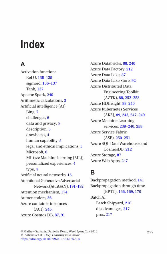
277
Index
AActivation functions
ReLU, 138–139sigmoid, 136–137Tanh, 137
Apache Spark, 240Arithmetic calculations, 3Artificial intelligence (AI)
Bing, 7challenges, 6data and privacy, 5description, 3drawbacks, 4human capability, 5legal and ethical implications, 5Microsoft, 6ML (see Machine learning (ML))personalized experiences, 4type, 4
Artificial neural networks, 15Attentional Generative Adversarial
Network (AttnGAN), 191–192Attention mechanism, 174Autoencoders, 36Azure container instances
(ACI), 245Azure Cosmos DB, 87, 91
Azure Databricks, 88, 240Azure Data Factory, 212Azure Data Lake, 87Azure Data Lake Store, 92Azure Distributed Data
Engineering Toolkit (AZTK), 88, 252–253
Azure HDInsight, 88, 240Azure Kubernetes Services
(AKS), 89, 243, 247–249Azure Machine Learning
services, 239–240, 258Azure Service Fabric
(ASF), 250–251Azure SQL Data Warehouse and
CosmosDB, 212Azure Storage, 87Azure Web Apps, 247
BBackpropagation method, 141Backpropagation through time
(BPTT), 166, 169, 170Batch AI
Batch Shipyard, 216disadvantages, 217pros, 217
© Mathew Salvaris, Danielle Dean, Wee Hyong Tok 2018 M. Salvaris et al., Deep Learning with Azure, https://doi.org/10.1007/978-1-4842-3679-6
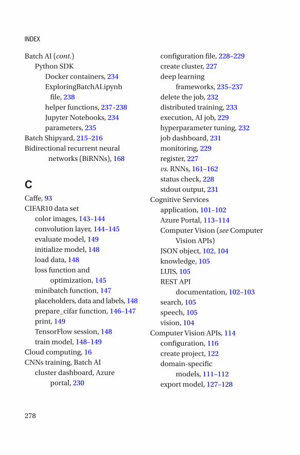
278
Python SDKDocker containers, 234ExploringBatchAI.ipynb
file, 238helper functions, 237–238Jupyter Notebooks, 234parameters, 235
Batch Shipyard, 215–216Bidirectional recurrent neural
networks (BiRNNs), 168
CCaffe, 93CIFAR10 data set
color images, 143–144convolution layer, 144–145evaluate model, 149initialize model, 148load data, 148loss function and
optimization, 145minibatch function, 147placeholders, data and labels, 148prepare_cifar function, 146–147print, 149TensorFlow session, 148train model, 148–149
Cloud computing, 16CNNs training, Batch AI
cluster dashboard, Azure portal, 230
configuration file, 228–229create cluster, 227deep learning
frameworks, 235–237delete the job, 232distributed training, 233execution, AI job, 229hyperparameter tuning, 232job dashboard, 231monitoring, 229register, 227vs. RNNs, 161–162status check, 228stdout output, 231
Cognitive Servicesapplication, 101–102Azure Portal, 113–114Computer Vision (see Computer
Vision APIs)JSON object, 102, 104knowledge, 105LUIS, 105REST API
documentation, 102–103search, 105speech, 105vision, 104
Computer Vision APIs, 114configuration, 116create project, 122domain-specific
models, 111–112export model, 127–128
Batch AI (cont.)
Index

279
giraffes, 124–127Hello World, 122–123image processing
techniques, 106–107intelligent zoo app, 122, 124keys, 116–117management, 116OCR, 110–111sample code, 117scenario, 119–120sign in, 120
Convolutional neural networks (CNNs), 28, 29
activation functionsReLU, 138–139sigmoid, 136–137Tanh, 137
architecture, 139CIFAR10 (see CIFAR10 data set)convolution layers
four, 152–154two, 151–152visualization, 134–135
deficiencies, 1355 × 5 matrix, 132–134MLPs, 142neuronal cells, 131parameter sharing, 143pooling layer, 135–136training process, 140–141transfer learning, 159
Custom Speech, 101Custom Vision, 101
Cycle-Consistent Adversarial Networks (CycleGANs)
adversarial loss, 206application, 194code
phase property, 197Python libraries, 196test method, 199train method, 199
cycle consistency loss, 206definition, 194generators and discriminators
network architecture, 202–204optimizer, 204–206
mapping functions, 195object transfiguration, 194–195
DData Science Virtual Machine
(DSVM), 86–87Decision making, 3Deep learning
applications, 21approaches, 16, 18, 20artificial neural network
models, 27autoencoders, 36business requirements, 39cloud computing, 19CNNs, 29comprehensive overview, 20data sets, 39–40, 99
Index

280
deploy, 42DNN, 16Facebook and Microsoft, 45finding data sets, 38GANs, 35GitHub, 46goals, 44GPUs and FPGAs, 16, 43hand-craft features, 15image, 14–15ImageNet data and
competition, 18Keras and Gluon, 44limitations, 20Microsoft Batch AI service, 47ML, 16mobile devices, 37models library, 50natural language processing, 15network structures, 28object detection, 37pretrained models, 45projects, 27–28research, 17ResNet-50, 47ResNet-152, 19R interfaces, 46RNNs, 33Rosetta Stone, 45semantics, 15speech recognition, 19speech-to-text APIs, 100supervised, 15
Tensorflow, 47traditional ML model, 20training, 40transfer learning and domain
adaptation, 47types of networks, 27validating and tuning, 40
Deep learning virtual machine (DLVM), 81, 213–214
Deep learning workspace (DL workspace), 217–218
Deep neural network (DNN) model, 15
Distributed training, 212–213, 225, 233
Domain Name Service (DNS), 96Domain-specific models, 111–112
EElectrocardiogram (ECG), 27Exploding gradients, 170
FFreezing layers, 160
GGenerative adversarial networks
(GANs), 28, 35adversarial loss, 188AI applications, 187algorithm, 188
Deep learning (cont.)
Index

281
AttnGAN, 191–192CycleGANs (see Cycle-
Consistent Adversarial Networks (CycleGANs))
deep learning, 190definition, 188discriminative model, 188generative model, 188image-to-image translations, 187InfoGAN, 190mode collapse, 193SeqGAN, 193StackGAN, 190text-to-image generation, 187working, 189
Graphical user interface (GUI), 92
HHDInsight (HDI), 254How-Old.net site, 108–109Hyperbolic tangent functions, see
Tanh functionsHyperparameter
tuning, 223–224, 232
IImageNet, 100, 160Image processing, 106–107Integrated development
environment (IDE), 93Intelligent zoo app, 122, 124Internet of Things (IOT), 42
JJupyter Notebooks, 234
KKubernetes cluster, 241
LLanguage Understanding
Intelligence Service (LUIS), 84, 105
Logistic function, see Sigmoid function
Long short term memory (LSTM), 34, 170–172
Loss functions, 141
MMachine learning (ML)
AI-infused applications, 9classical approaches, 9, 13customers and demographic
data, 10data representation, 11feature engineering, 9personalized experiences, 12predictive maintenance
solutions, 12preprocessing, 11supervised approach, 10–13tasks, 9
Max pooling layer, 30
Index
282
Microsoft AI PlatformAzure Machine Learning
services, 84Batch AI, 85bot framework, 84cloud computing, 79, 80cognitive services, 82data storage, 91deep learning solution, 80development environments, 80DLVM, 81DSVM, 87hosting, 89infrastructure, 86Machine Learning Server, 79open-source technology, 80services, 81Spark, 88SQL Server, 79tools
Azure Machine Learning Studio, 92
Broader Azure Platform, 94deep learning
frameworks, 93Deep Learning Virtual
Machine, 95IDE, 93Notebook Server, 97
Microsoft Cognitive Toolkit (CNTK), 46, 93
Microsoft Machine Learning for Apache Spark (MMLSpark), 89, 240
Microsoft stock, LSTMhyperparameters, 181normalize data, 181reshaping data, 182RMSE, 183, 185train and test sets, 181training model, 182
Multi-instance tasks, 225Multilayer perceptrons
(MLPs), 29, 142
NNatural language
processing, 19, 22–23, 49Network architecture, 16Neural machine translation
(NMT), 172–173
OOperationalization, AI models
ACI, 245–246AKS, 247–249ASF, 250–251AZTK, 252–253Azure Web Apps, 247Batch AI, 251–252batch to real-time
continuum, 256DLVM, 245HDInsight and Databricks, 254heatmap of deployment
services, 257
Index
283
platforms, 243–244SQL Server, 255
Optical Character Recognition (OCR), 110–111
P, QPooling layer, 135–136Public data sets, 99PyTorch, 93
RRealtime Crowd Insights, 109–110Rectified linear unit
(ReLU), 138–139Recurrent neural networks
(RNNs), 28, 33architectures
asynchronous many-to- many pattern, 165
backward propagation, 166BiRNNs, 168design patterns, 164–165many-to-one pattern, 164nonlinear function, 165one-to-many pattern, 164output recurrent
structure, 166–167vanilla neural
network, 164–165BPTT, 169vs. CNNs, 161–162exploding gradients, 170
image classificationargmax() operation, 180create network
architecture, 177loading data, 177placeholders and initialize
variables, 178supply data to model, 179–180training model, 179
Microsoft stock (see Microsoft stock, LSTM)
one-hot encoded vectors, 163sentiment analysis, 176summing input vectors, 163–164training method, 169–170vanishing gradients, 170
Reinforcement learning, 20Root mean squared error
(RMSE), 183, 185
SScale-invariant feature transform
(SIFT), 31Sequence-to-sequence
models, 172–175Sigmoid function, 136–137Software Development Kit
(SDK), 84Spark clusters, 86Speech-to-speech translation, 4SQL Data Warehouse, 87Stacked Generative Adversarial
Networks (StackGAN), 190
Index
284
Stochastic gradient descent (SGD), 141
Supervised deep learning models, 15Supervised machine
learning, 9, 10, 12
T, UTanh functions, 137Tensorflow, 93Training AI models
Apache Spark, 240Batch AI (see Batch AI)Batch Shipyard, 215–216distributed training, 212–213DLVM, 213–214DL workspace, 217–218Kubernetes clusters, 241MMLSpark, 240
Training DNN, Batch ShipyardAI script execution, 218–219Azure portal, 222command to create batch
cluster, 221configuration files, 220create azure resources, 220distributed training, 225hyperparameter
tuning, 223–224review errors and debug
scripts, 222submit job, 222
Transfer learning, 47, 159–160
V, W, X, Y, ZVanishing gradients, 170Virtual machines (VM), 40
Index