deformation analysis of sand specimens using 3d …
TRANSCRIPT

DEFORMATION ANALYSIS OF SAND SPECIMENS USING 3D DIGITAL IMAGE
CORRELATION FOR THE CALIBRATION OF AN ELASTO-PLASTIC MODEL
A Dissertation
by
AHRAN SONG
Submitted to the Office of Graduate Studies of Texas A&M University
in partial fulfillment of the requirements for the degree of
DOCTOR OF PHILOSOPHY
August 2012
Major Subject: Civil Engineering

Deformation Analysis of Sand Specimens using 3D Digital Image Correlation for the
Calibration of an Elasto-Plastic Model
Copyright 2012 Ahran Song

DEFORMATION ANALYSIS OF SAND SPECIMENS USING 3D DIGITAL IMAGE
CORRELATION FOR THE CALIBRATION OF AN ELASTO-PLASTIC MODEL
A Dissertation
by
AHRAN SONG
Submitted to the Office of Graduate Studies of Texas A&M University
in partial fulfillment of the requirements for the degree of
DOCTOR OF PHILOSOPHY
Approved by:
Chair of Committee, Zenon Medina-Cetina Committee Members, Marcelo Sanchez Chloe Arson Javier Jo Gokhan Saygili Head of Department, John Niedzwecki
August 2012
Major Subject: Civil Engineering

iii
ABSTRACT
Deformation Analysis of Sand Specimens using 3D Digital Image Correlation for the
Calibration of an Elasto-Plastic Model. (August 2012)
Ahran Song, B.S., Sungkyunkwan University, South Korea;
M.S., Sungkyunkwan University, South Korea
Chair of Advisory Committee: Dr. Zenon Medina-Cetina
The use of Digital Image Correlation (DIC) technique has become increasingly
popular for displacement measurements and for characterizing localized material
deformation. In this study, a three-dimensional digital image correlation analysis (3D-
DIC) was performed to investigate the displacements on the surface of isotropically
consolidated and drained sand specimens during triaxial compression tests.
The deformation of a representative volume of the material captured by 3D-DIC
is used for the estimation of the kinematic and volumetric conditions of the specimen at
different stages of deformation, combined with the readings of the global axial
compression of the specimen. This allowed for the characterization of a Mohr-Coulomb
plasticity model with hardening and softening laws.
In addition, a two-dimensional axisymmetric finite element model was built to
simulate the actual experimental conditions, including both the global and local
kinematics effects captured by 3D digital image correlation analysis on the boundary of
the specimen.

iv
A comparison between the axisymmetic model predictions and the experimental
observations showed good agreement, for both the global and local behavior, in the case
of different sand specimen configuration, including loose, dense and half-loose half-
dense specimens.

v
DEDICATION
To my family

vi
ACKNOWLEDGEMENTS
I would like to thank my committee chair, Prof. Zenon Medina-Cetina for his
guidance and provision of financial assistance, and my committee members, Prof.
Marcelo Sanchez, Prof. Chloe Arson, Prof. Javier Jo, and Dr. Gokhan Saygili for their
sincere advice and support throughout the course of this research.
Thanks are also extended to my friends in geotechnical engineering and
colleagues in stochastic geomechanics laboratory group for making my time at Texas
A&M University a great experience. I am really grateful to Patricia and Vishal for
sharing the happy moments as reliable friends and to Patrick for spending his valuable
time to proofread this thesis. Also, I will remember warm and friendly Korean students
and their families, especially Seok-gyu who would take care of me all the time.
Finally, thanks to my family for their encouragement and support and to Naoki
for his patience during my studies.

vii
TABLE OF CONTENTS
Page
ABSTRACT .............................................................................................................. iii
DEDICATION .......................................................................................................... v
ACKNOWLEDGEMENTS ...................................................................................... vi
TABLE OF CONTENTS .......................................................................................... vii
LIST OF FIGURES ................................................................................................... ix
LIST OF TABLES .................................................................................................... xiv
1. INTRODUCTION ............................................................................................... 1
1.1 Antecedents .......................................................................................... 1 1.2 Proposed Approach .............................................................................. 3
2. SOIL EXPERIMENTATION ............................................................................. 5
2.1 Triaxial Testing .................................................................................... 5 2.2 3D Digital Image Correlation Analysis ................................................ 13 2.2.1 Digital Image Correlation ............................................................ 13 2.2.2 Qualitative Assessment of Localization Effects .......................... 18
3. 3D DIGITAL IMAGE TRANSFORMATIONS AND INTERPOLATION ...... 25
3.1 Digital Image Corrections .................................................................... 25 3.2 Assessment of the Trend Fitting Plane ................................................. 26 3.3 3D Geometrical Transformations ......................................................... 27 3.3.1 Rotation Analysis ........................................................................ 27 3.3.2 Translation Analysis .................................................................... 32 3.3.3 Trend Fitting Plane Coefficients and Rotation Analysis ............. 34 3.4 Interpolation of Image Data ................................................................. 37 3.4.1 Interpolation and Extrapolation for Cumulative Displacement Fields ........................................................................................... 37 3.4.2 Interpolation for Corrections of Incorrect Image Data ................ 40 3.5 Cumulative Displacement Fields ......................................................... 41 3.6 Cumulative Strain Fields ...................................................................... 48

viii
Page
3.7 Volumetric Strain ................................................................................. 50
4. SIMPLE ONE ELEMENT MODEL TEST ........................................................ 55
4.1 Calibration of Model Parameters ......................................................... 55 4.2 One Element Model Test Cases ........................................................... 56 4.3 Boundary and Loading Conditions ...................................................... 58 4.4 Stress and Strain Behavior ................................................................... 62 4.5 Hardening and Softening Analysis ....................................................... 67 4.5.1 Stress and Strain Relationship in the Hardening and Softening Curve ........................................................................................... 67 4.5.2 Determination of the Hardening and Softening Parameters ........ 69 4.5.3 Quadratic Spline Interpolation .................................................... 71
5. CASE STUDY .................................................................................................... 73
5.1 Simulation of the Compression Triaxial Test ...................................... 73 5.2 Homogeneous Material Tests for a Dense Sand Specimen .................. 74 5.2.1 Local Deformation Effects from a Dense Sand Specimen .......... 74 5.2.2 Local Deformation of Homogeneous Materials .......................... 75 5.3 Mesh Sensitivity Analysis in Plastic Straining .................................... 79 5.3.1 Problem Definition ...................................................................... 79 5.3.2 Effects of Mesh Discretization .................................................... 82 5.3.3 Effects of Element Type .............................................................. 84 5.3.4 Effects of Mesh Size ................................................................... 86 5.3.5 Stress and Strain Cross Sections ................................................. 91 5.4 Comparative Analysis among Dense, Loose, and Layered Sand Specimens ............................................................................................. 93 5.4.1 Experimental Comparison ........................................................... 93 5.4.2 2D Axisymmetric Finite Element Modeling ............................... 97 5.4.3 Comparative Results ................................................................... 100
6. CONCLUSIONS ................................................................................................. 105
REFERENCES .......................................................................................................... 107
VITA ......................................................................................................................... 115
ix
LIST OF FIGURES
Page
Figure 2. 1 Triaxial Geocomp system (a), and 3D imaging system (b) (Medina-Cetina 2006) ............................................................................... 6 Figure 2. 2 Triaxial stress-strain curves for all tests ................................................. 10 Figure 2. 3 Mohr's circles of triaxial tests for dense specimens ................................ 12 Figure 2. 4 Curved failure envelope and friction angles at failure for dense specimens ................................................................................................... 13 Figure 2. 5 Photo images of test 120904c at (a) 0.2% of axial strain (b) 3.6% of axial strain (c) 7% of axial strain (d) 12% of axial strain .......................... 14 Figure 2. 6 Reference image (a) area of interest (b) seed windows (VIC-3D) ........ 15 Figure 2. 7 Common section captured by the VIC-3D two cameras system (a and b) and displacement fields in 2D and 3D shapes (c) ..................................... 16 Figure 2. 8 Incremental displacement fields of test 120904c between 2.8% and 3.0% of axial strain, obtained by 3D-DIC process: (a) u field (b) v field (c) w field ................................................................................................... 17 Figure 2. 9 Accuracy analysis: (a) comparison of displacement measurements between triaxial test system and VIC-3D (b) absolute frequency histogram of absolute error of displacement measurements between triaxial test system and VIC-3D (Medina-Cetina 2006) ............................ 18 Figure 2.10 Digital image and corresponding incremental displacement fields at 12% of axial strain (a) photo image (b) u field (c) v field (d) w field ........ 20 Figure 3. 1 Code for finding an equation of a fitting plane ....................................... 27 Figure 3. 2 3D geometrical transformation process (a) normal vectors in space (b) rotation process ..................................................................................... 29 Figure 3. 3 Schematic view of 3D transformations: rotation .................................... 29 Figure 3. 4 Code for rotation process ........................................................................ 29

x
Page
Figure 3. 5 Geometrical transformation of 10 data points (a) xyz view (b) x-z view ................................................................................................ 31 Figure 3. 6 Geometrical transformation of test 120904b (a) before rotations (b) after rotations ........................................................................................ 31 Figure 3. 7 Translation on y- and z- directions (a) y-direction translation (b) z-direction translation ........................................................................... 33 Figure 3. 8 Schematic view of 3D transformations: translation ................................ 33 Figure 3. 9 Code for translation in y- and z-directions ............................................. 33 Figure 3. 10 Result of test 120904b after translation on y- and z- directions ........... 34 Figure 3. 11 Data plots and a fitting plane in x-z plane for test 120904c (a) before rotation (b) after rotation ............................................................................ 35 Figure 3. 12 Rotation angle analysis (a) rotation angles of each test (b) frequency histogram of rotation angle ........................................................................ 37 Figure 3. 13 Scheme of interpolation and extrapolation ........................................... 39 Figure 3. 14 Interpolation and extrapolation between image no.000 and no.008 (0.4% of axial strain) ................................................................................. 39 Figure 3. 15 Total displacement fields of test 120904c (a) undeformed state (b) deformed state at 0.4% of axial strain .................................................. 40 Figure 3. 16 Correction of light reflection problem for test 120704c ....................... 41 Figure 3. 17 Correction of incorrect data generated by shearing plane for test 121304d ............................................................................................... 41 Figure 3. 18 Cumulative displacement fields of test 120904c in Cartesian coordinate system at 0.2%, 3.6%, 7%, and 12% of axial strain: (a) horizontal (u) displacement field (b) vertical (v) displacement field (c) out-of-plane (w) displacement field ................................................................................ 44 Figure 3. 19 Cumulative displacement fields of test 120904c in cylindrical coordinate system at 0.2%, 3.6%, 7%, and 12% of axial strain: (a) radial displacement field (b) tangential displacement field (c) axial displacement field .......... 45

xi
Page
Figure 3. 20 Averaged displacements of test 120904c (a) radial displacement (b) vertical displacement ............................................................................ 46 Figure 3. 21 Conversion between Cartesian and cylindrical coordinate systems ..... 47 Figure 3. 22 Cumulative strain fields of test 120904c at 0.2%, 3.6%, 7%, and 12% of axial strain: (a) 11 field (b) 22 field (c) 12 field ...................................... 49 Figure 3. 23 Process for averaging radius and uniformalizing height ...................... 51 Figure 3. 24 Averaged radius profile for test 120904c at (a) 0.2% of axial strain (b) 3.6% of axial strain (c) 7% of axial strain (d) 12% of axial strain ....... 53 Figure 3. 25 Axial strain vs. volumetric strain curve of test 120904c ...................... 54 Figure 3. 26 Code for volume calculation ................................................................. 54 Figure 4. 1 Global stress-strain behavior of test 120904c (a) stress vs. strain curve (b) axial strain vs. volumetric strain curve ................................................. 56 Figure 4. 2 Applied loading steps on the one element model ................................... 59 Figure 4. 3 Mean stress contour at different loading steps ........................................ 59 Figure 4. 4 Vertical displacement contour at different loading steps ........................ 60 Figure 4. 5 Stress paths in p-q plane (a) four loading steps condition of test One_ pk (b) two loading steps condition of test One_pk_step ................................. 61 Figure 4. 6 Comparison of stress-strain behavior of an elasto-perfectly plastic model with different friction angles at peak and critical state ............................. 63 Figure 4. 7 Comparison of stress-strain behavior between an elasto-perfectly plasticity model and an elasto-plasticity model ......................................... 64 Figure 4. 8 Mohr-Coulomb yield surface in meridional and deviatoric planes (ABAQUS user’s manual 2008) ............................................................... 66 Figure 4. 9 Hardening and softening curve (a) concept of experimental data points (b) generated smooth hardening and softening curve ................................ 70 Figure 4. 10 Code for calculation of the coefficients of a quadratic spline .............. 72 Figure 5. 1 2D axisymmetric finite element full model ............................................ 74

xii
Page
Figure 5. 2 Cumulative displacement fields at (a) 0.2% of axial strain (b) 3.6% of axial strain (c) 7% of axial strain (d) 12% of axial strain .......................... 75 Figure 5. 3 Hardening and softening curve for homogeneous materials................... 77 Figure 5. 4 Global stress-strain behavior of homogeneous materials ....................... 78 Figure 5. 5 Displacements and cumulative density function at 3.6% and 7% of axial strain (a) radial displacement (b) cumulative density function of radial displacement errors (c) axial displacement (d) cumulative density function of axial displacement errors ......................................................... 79 Figure 5. 6 Mesh discretization of 2D finite element models (a) 3mm_tr, 3mm_sq (b) 5mm_tr, 5mm_sq (c) 10mm_tr, 10mm_sq (d) 20mm_tr, 20mm_sq (e) 40mm_tr, 40mm_sq .............................................................................. 83 Figure 5. 7 Effects of element type on global stress-strain behavior ....................... 85 Figure 5. 8 Effects of mesh size on global stress-strain behavior ............................ 87 Figure 5. 9 Displacements and displacement errors at peak: (a) radial displacement (b) radial displacement errors (c) vertical displacement (d) vertical displacement errors .................................................................................... 88 Figure 5. 10 Displacements and displacement errors at critical state: (a) radial displacement (b) radial displacement errors (c) vertical displacement (d) vertical displacement errors .................................................................. 90 Figure 5. 11 Deformed meshes with horizontal displacement contour ..................... 91 Figure 5. 12 Deviatoric stress and plastic strain distribution of test 3mm_sq_8 at peak and critical state (a) deviatoric stress (b) plastic strain .................. 92 Figure 5. 13 3D digital image correlation analysis at 0.2% of axial strain (elastic state) .............................................................................................. 94 Figure 5. 14 3D digital image correlation analysis at 12% of axial strain (critical state) ............................................................................................. 95 Figure 5. 15 Comparison between experimental results (a) deviatoric stress vs. axial strain curve (b) volumetric behavior vs. axial strain ......................... 96

xiii
Page
Figure 5. 16 Sand specimen configurations (a) dense specimen (b) loose specimen (c) layered specimen modeled with a homogeneous material (layered_hom) (d) layered specimen consists of two layers (layered_het) (e) layered specimen considering a transition zone (layered_het_transition) ............. 97 Figure 5. 17 Hardening and softening curves for (a) dense specimen (b) loose specimen, upper loose segment of layered_het model, and layered_hom model .................................................................................... 100 Figure 5. 18 Model predictions in global behavior for dense and loose specimens.. 101 Figure 5. 19 Model predictions in global behavior for a layered specimen .............. 101 Figure 5. 20 Radial displacement distributions and its errors (a) radial displacement distribution (b) radial displacement errors ................................................. 102 Figure 5. 21 Vertical displacement distributions and its errors (a) vertical displacement distribution (b) vertical displacement errors ........................ 103 Figure 5. 22 Total displacement vectors (a) layered_hom (b) layered_het (c) layered_het_transition ........................................................................... 104

xiv
LIST OF TABLES
Page Table 2. 1 Experimental characteristics of triaxial tests ............................................ 7 Table 3. 1 Plane coefficients and rotation angle analysis (plane equation: z=ax+bx+c) ..................................................................... 36 Table 4. 1 One element model test cases and material properties ............................. 57 Table 5. 1 Summary of model parameters for homogeneous materials .................... 76 Table 5. 2 Test cases for mesh sensitivity analysis ................................................... 83 Table 5. 3 Coefficients for an estimation of the friction angle (Duncan, J.M. 2004) .................................................................................. 98 Table 5.4 Summary of material properties for dense, loose and layered specimens 99

1
1. INTRODUCTION
1.1 Antecedents
Duncan’s state of the art review (1994) on advanced constitutive models
provided important key points on the limitations that practice have on the modeling of
geotechnical structures. Lade’s state of the art review (2005) went further and provided
a more specific overview of the principles, characteristic features, and requirements for
the calibration of constitutive models, for the proper model selection and implementation
in advanced case studies. Potts and Zdravkovic (1999) reviewed various methods of
analysis including from closed form to full numerical analysis in terms of the
fundamental theoretical solutions, and also provided the ability of each method to satisfy
the design requirements. Hicher and Shao (2008) rearranged several failure criteria and
suggested the appropriate type of soils for each criterion that is validated by
experimental results for a different type of soils. Also, Brinkgreve (2005) stated a
difficulty of the selection of soil parameters in terms of insufficient data from correlation
and laboratory testing for application in finite element soil models. All these
contributions, ignored the effect of material heterogeneity and local kinematic effects at
the time of calibrating the constitutive models. Meaning that only considered the global
stress and strain effects captured on the axial direction of the specimens.
This dissertation follows the style and format of the Journal of Geotechnical and Geoenvironmental Engineering.

2
Digital image correlation (DIC) is one of the most widely used optical techniques
for full displacement measurements, allowing for the identification and characterization
of local kinematic effects. DIC developed basically for the characterization of material
deformations in the early 1980s, and since then the DIC concept has been extended from
2D DIC using a single camera system, to 3D-DIC using a multi camera system. The
major progress on the use of DIC technology can be located in the early 1990s, with
advances in the quality of digital camera and computational capabilities (McNeill et al.
1997; Sutton et al. 2000; Sutton et al. 2008). Recently, more elaborated studies of the
3D-DIC technique have been dedicated to improved previous 2D DIC dealing with
planar surfaces, in-plane deformations, and perpendicular camera setting to the object
surface (Sutton et al. 2008). Nowadays, the development of the 3D-DIC technique
permits to measure anisotropic, volumetric and heterogeneous strains (Almeida et al.
2008). For instance, in order to improve the understanding of specimens’ failure
mechanisms, a 3D-DIC system was implemented for investigating shear and compaction
bands in sand specimens (Desrues and Viggiani 2004; Rechenmacher 2006;
Charalampidou et al. 2010), showing even at the grain level, the kinematics of these
effects. Notice that in the case of a 3D-DIC system using only two cameras, the
measurement area for a cylindrical sample is expected to be approximately one third of
the circumference due to the maximum overlap area between any given pair of images
(Tai et al. 2010).
What these investigations have in common is that they found significant
heterogeneous responses in apparently homogeneous specimens, and suggested various

3
methods for better understanding the effect of full boundary displacement fields.
Although previous research has provided valuable information for the understanding of
DIC implementation, further research is still required on its incorporation on standard
model calibration (Medina-Cetina and Rechenmacher 2010).
Herein, once the notion of incorporating local deformation effects into the
calibration process has been discussed, it is fair to mention that the selection of a soil
constitutive model itself and its corresponding calibration process are not simple tasks to
complete. This process is dependent on several conditions, including its ability to
capture the physics associated to the particular application where the model is going to
be used, its easiness to apply it, its availability in a numerical solver (i.e. commercial
finite element codes), and its feasibility for calibration purposes, among others (Duncan
1994; Potts 2003; Brinkgreve 2005; Lade 2005; Boldyrev et al. 2006).
1.2 Proposed Approach
This work is based on the population of a comprehensive experimental database
containing a series of triaxial compression tests on sand specimens performed by
Medina-Cetina (2006). This work aims at computing the collected 3D digital image data
from the surface of soil specimens using 3D-DIC. That is to generate 3D local
kinematic information that is retrieved during a compression test over the surface of the
deforming specimen. A comprehensive investigation into the localized deformation of
sand specimens using 3D digital image correlation (3D-DIC) is carried out including 3D
geometrical transformation and interpolation/extrapolation processes with the aim of

4
identifying the global behavior of the specimen. From the kinematic and volumetric
conditions of the specimen at different stages of deformation, combined with the
corresponding readings of the global axial compression of the specimen, this work aims
at characterizing simple elasto-plastic constitutive models for quantifying their
advantages and limitations for prescribed experimental conditions.
To achieve this goal, first, a qualitative analysis is presented describing typical
failure mechanisms on a series of dry sand triaxial specimens; second, a simple elasto-
plastic constitutive model with hardening and softening capabilities is calibrated using a
single finite element; and finally, a 2D finite element model is developed for comparing
the actual experimental results. Results on the modeling of local kinematics effects,
demonstrate the ability of the proposed constitutive model to reproduce accurately the
overall mechanical behavior of a sand specimen under the given conditions. This
approach is further extended for the case of true heterogeneous materials, proving the
relevance of accounting for spatial variability of the elasto-plastic constitutive
parameters within the numerical model. The calibration process to determine
constitutive model parameters is discussed for comparing actual triaxial testing data and
numerical predictions when material heterogeneity and evolutionary material
degradation is considered. By means of this calibration methodology that accounts for
the model performance of soil constitutive models, it can be a meaningful way to
determine what constitutive model provides better predictions and practical solutions to
the actual soil behavior, when observations on local kinematic effects are available.

5
2. SOIL EXPERIMENTATION
2.1 Triaxial Testing
The triaxial test and 3D imaging systems setup used to populate the experimental
database is presented in Figure 2.1 (Medina-Cetina 2006). A departure from standard
triaxial tests was the removal of the Plexiglass cell to avoid reflection and refraction
effects by light and fluid, respectively. This means that tests were conducted on sand
specimens vacuum consolidated, instead of fluid-based consolidation during the image
acquisition. An automated triaxial device developed by Geocomp was used to execute
the compression tests and to measure the global stress-strain axial response. The 3D
imaging system consisted of two digital cameras positioned approximately 25cm from
each other, and 50cm from the sample as shown in Figure 2.1 (b).
The material for the triaxial compression test was a dry sand, classified as SP,
having Cu=2.34 and Cc=1.11, and provided an adequate color spectrum suitable for
pattern recognition during imaging analysis. A specimen was constructed using a
standard cylindrical mold following dry pluviation or vibratory compaction methods
reaching a relative density varying between 83 and 99% for dense sand specimens and
46% for a loose sand specimen (test 121304b). After the specimen setup, the mold was
removed and an isotropic compression of vacuum pressure was applied to the base of the
sample with a vacuum pump in order to keep the sample stable. The specimen was
loaded with a controlled deformation rate of 0.2% of axial strain/min.

6
Figure 2. 1 Triaxial Geocomp system (a), and 3D imaging system (b) (Medina-Cetina 2006)
The experimental characteristics of all triaxial tests included in the database are
presented in Table 2.1. This shows the results of twenty seven experiments, classified as
follows: twenty five dense specimens, one half loose and half dense specimen (test
120704c), and one loose sand specimen (test 121304b). Most specimens were
consolidated at 40kPa of vacuum pressure, but three tests were consolidated at a
confining pressure of 20kPa (test 121304d) and 60kPa (100103c and 121304c tests)
respectively. The average diameter of all specimens was 71.15 mm with a standard
deviation of 0.27 mm, and the corresponding average height was 158.31 mm, with a
standard deviation of 1.62 mm. After excluding the data of a layered specimen and a
loose sand specimen, the dense specimens’ average initial density was 1,712.89 kg/m3
with a standard deviation of 10.10kg/m3, and the corresponding average relative density
was 91.72% with a standard deviation of 3.43% respectively. From all experiments,
eighteen samples were prepared in three layers by a vibratory compaction method and

7
eight samples were prepared by a dry pluviation method. The layered specimen (half
loose and half dense) was built in two compacting layers, with the lower half dense layer
with relative density of 98.87% and the upper loose layer with relative density of
30.54%. The boundary of two layers was located at the mid height of the specimen.
Table 2. 1 Experimental characteristics of triaxial tests
No. Test Name
Height (mm)
Diameter (mm)
Initial Density (kg/m3)
Relative Density
(%) Sample
Preparation Note
1 092903b 155.50 71.33 1,710.95 91.09 Mold tempered -
2 093003b 156.67 71.41 1,696.00 85.96 Mold tempered -
3 100103a 157.67 71.29 1,702.22 88.10 Mold tempered -
4 100103b 155.83 71.24 1,717.13 93.18 Mold tempered -
5 100103c 157.67 71.54 1,703.87 88.67 Mold tempered 60kPa confinement
6 100103d 154.33 70.86 1,702.41 88.17 Mold tempered -
7 100203a 157.50 71.45 1,715.32 92.57 Mold tempered -
8 100203b 155.00 71.48 1,711.91 91.41 Mold tempered -
9 100303b 158.17 71.29 1,718.70 93.71 Mold tempered -
10 101104a 159.33 70.87 1,724.89 95.79 Dry Pluviation Light reflection
11 101204a 160.00 71.46 1,708.03 90.09 Dry Pluviation -
12 120604a 159.33 71.31 1,721.06 94.50 Dry Pluviation Light reflection
13 120604b 159.33 70.94 1,715.13 92.50 Dry Pluviation Light reflection
14 120604c 158.83 70.72 1,717.48 93.30 Mold tempered Light reflection
15 120604d 158.83 70.84 1,716.99 93.13 Mold tempered Light reflection
16 120704a 158.83 71.37 1,708.07 90.11 Mold tempered Light reflection

8
Table 2. 1 continued
No. Test Name
Height (mm)
Diameter (mm)
Initial Density (kg/m3)
Relative Density
(%) Sample
Preparation Note
17 120704b 159.00 71.30 1,686.96 82.82 Mold tempered Light reflection
18 120704c
157.67 70.88 1,648.06 68.90 Mold tempered Layered specimen
79.50 71.27 1,734.17 98.87 - Lower: dense sand
78.17 70.68 1,549.61 30.54 - Upper: loose sand
19 120904a 158.67 71.15 1,707.72 89.99 Mold tempered Light reflection
20 120904b 160.00 70.98 1,720.40 94.28 Mold tempered -
21 120904c 159.67 71.11 1,713.13 91.83 Mold tempered -
22 120904d 159.00 71.13 1,707.89 90.04 Mold tempered -
23 120904e 160.00 70.99 1,718.70 93.71 Mold tempered -
24 121304a 160.00 71.30 1,721.73 94.73 Dry Pluviation -
25 121304b 158.17 70.86 1,588.84 46.39 Dry Pluviation Loose specimen
26 121304c 160.00 70.48 1,718.72 93.72 Dry Pluviation 60kPa confinement
27 121304d 159.50 71.38 1,736.71 99.71 Dry Pluviation 20kPa confinement
For the sample in a water-filled cell, the cell pressure supplies a uniform radial
stress, r, and an additional force, Fa, is measured by a force transducer. If the cross-
sectional area of the sample is A, then the total axial stress, a is given by a=r+(Fa/A).
The deviatoric stress, d, is calculated by d=a-r=(Fa/A) (Atkinson and Bransby, 1978).
Although dry samples were used for experiments, the test setup satisfies conditions of a
conventional drained triaxial compression test. The cell pressure was constant and a

9
change of volume was allowed while the deviatoric stress increased. Thus, the
calculated deviatoric stress is considered in an effective stress.
Global stress-strain curves for all tests are presented in Figure 2.2. For dense
sand specimens with a confining pressure of 40kPa, the maximum deviatoric stress
oscillated between 220 and 255kPa, and the deviatoric stress at the critical state ranged
between 155 and 185kPa. For the two tests with a confining pressure of 60kPa, the
deviatoric stresses were 317~359kPa at peak and 265~270kPa at critical state. It is
hypothesized that deviations in deviatoric stress with the same confinement condition
were caused by the variation of relative density within the specimen as a results of the
sample preparation methods. The loose specimen test has no peak stress and yields to
150kPa from 3.2% of axial strain to the critical state. The layered specimen test does not
have a typical behavior of a dense sand specimen and shows the behavior of a loose sand
specimen.

10
Figure 2. 2 Triaxial stress-strain curves for all tests
Although a dry sample is prepared, the specimen is exposed to the atmospheric
air pressure and moisture. This explains the existence of cohesion with respect to matric
suction. The shear strength of saturated soils for the Mohr-Coulomb theory is defined as
wτ=c'+(σ-u )tan ' , where c’ is effective cohesion. The shear strength of unsaturated soils
is proposed by Fredlund et al. (1996) as a wτ=c'+(σ-u )tan '+(u -u )βtan 'a , where ua is the
pore-air pressure, uw is the pore-water pressure, a w(u -u ) is matric suction, and β

11
represents the decrease in effective stress resistance as matric suction increases. β is
dependent on the water content of soil and expressed as being equal to tan / tan 'b .
From the equation, a w[(u -u )βtan '] part is defined by Peterson (1988) as an apparent
cohesion due to suction and it explains the cohesion of the specimen.
However, for the soils above the groundwater level, a conventional saturated soil
mechanics concept is generally sufficient for engineering purposes (Powrie 1997). Thus,
the assumption of zero cohesion can be acceptable in this study. The parameter, β
depends on the saturation ratio and varies from 0 for dry soils to 1 for saturated soils
(Powrie 1997; Nuth and Laloui 2008). Assuming a dry sample of the tests, the strength
equation becomes τ=(σ-u )tan 'a . If ua is replaced with r which is vacuum pressure for
the dry sample compared with the deviatoric stress form presented above, using vacuum
compression as a confining pressure is allowed for the effect stress analysis.
Mohr’s circles for experiments on dense sand specimens are illustrated in Figure
2.3. From these result, under the assumption that the cohesion is equal to zero, it is
observed that an averaged friction angle at peak strength is calculated as 48.46° with a
standard deviation of 0.85°.
A failure envelope and friction angles at the peak strength for dense sand
specimens are presented in Figure 2.4. Peak strength data plotted as normal stress vs.
shear stress shows a curved failure envelope as seen in Figure 2.4 (a). The friction angle
at peak strength is found by means of a best fit straight line, having an equation of the
form, =c+tan, where c is assumed to be equal to zero here for sand specimens. This
assumption leads to the overestimation of the actual peak strength at low stress,

12
depending on how to draw the best fit line (Holtz and Kovacs 1981; Powrie 1997). This
results in an apparent peak friction angle higher than the average friction angle at low
confining stress, and even lower at high confining stress (Figure 2.4 (b)). Vesic and
Clough (1968) depicted this behavior of dense and loose sand specimens with respect to
pressure sensitivity. The friction angle of loose samples was the same at different stress
levels, but the friction angle of dense samples was sensitive at a low stress level and
constant at a high stress level.
Figure 2. 3 Mohr's circles of triaxial tests for dense specimens

13
Figure 2. 4 Curved failure envelope and friction angles at failure for dense specimens
2.2 3D Digital Image Correlation Analysis
2.2.1 Digital Image Correlation
A digital image correlation technique is a reliable and accurate approach for the
investigation of local kinematics, aimed at capturing local phenomena of deforming
specimens. 3D digital image correlation (3D-DIC) is developed based on principles
similar to human eye’s depth perception, viewing the same object from two different
viewpoints and judging distance. An innovative qualitative interpretation of the
specimen deformation is provided by the use of digital images, which are taken
simultaneously every 15 seconds corresponding to 0.05% of axial strain during the
triaxial compression test using two 14-bit digital cameras Q-IMAGING PMI-4201, with
4.2 Mega pixels of resolution (2024×2024 pixels). Sample images that capture the state
of the sample at deformation stages of 0.2%, 3.6%, 7% and 12% of axial strain by one

14
digital camera are shown in Figure 2.5. These images illustrate amplification of bulging
failure procedure as the state of the sample at the elastic zone, peak stress, softening
zone, and critical state, respectively.
Figure 2. 5 Photo images of test 120904c at (a) 0.2% of axial strain (b) 3.6% of axial strain (c) 7% of axial strain (d) 12% of axial strain
Commercial software VIC-3D, a digital image correlation (DIC) system,
developed by Correlated Solutions Inc. was used to digitalize the photo images and to
assimilate the images into 3D full-field displacements, as captured from the surface of
the specimen. For the correlation analysis to be performed, VIC-3D requires the
selection of an area of interest and a seed window at the first set of images. An area of
interest is where displacements are quantified and a seed window is defined as the
common pixels that are clearly identified in order to obtain an initial guess for the next
images, on both left and right images as shown in Figure 2.6. A subset of 45 pixels and
a step size of 3 pixels were selected to achieve as close to grain-scale resolution in the
displacement measurement as possible.

15
Figure 2. 6 Reference image (a) area of interest (b) seed windows (VIC-3D)
Once the 3D imaging system is calibrated and the reference image is prepared for
analysis, VIC-3D can perform the 3D surface reconstruction. The common section
captured by two cameras is where the displacement fields are analyzed which accounts
for 40~50 mm horizontal width, which is equivalent to about one third of the
circumstance of the specimen from the top view (Figure 2.7 (a) and (b)). VIC-3D
generates 2D and 3D contour plots of the displacement fields available in the common
section. The gray scale image of the 2D plot displays the lost data area while the color
image displays the value of the current contour variable as well as the 3D plot.
Horizontal displacement fields at 12% of axial strain for test 120904c are presented in
2D and 3D shapes Figure 2.7 (c).

16
Figure 2. 7 Common section captured by the VIC-3D two cameras system (a and b) and displacement fields in 2D and 3D shapes (c)
The tests recorded deformation data up to 12% of the axial strain, from which it
was impossible to trace local deformations with respect to the undeformed state. To
overcome this problem, the 3D-DIC system VIC-3D, updated the reference images for
every 4th image, i.e. every 0.2% of axial strain, thus incremental displacements were
computed. For example, Figure 2.8 illustrates the incremental displacement fields at 3.0%
of axial strain when the reference image is the image at 2.8% of axial strain. The
orientation of the system setup is described in a global Cartesian system, and u, v, and w
are displacements corresponding to x, y, and z directions respectively. Then, in order to
measure cumulative displacement fields and impose the finite element displacement
17
fields on digital images, it was required to develop a numerical integration of each
sequential 3D-DIC. A detail description about this integration is presented later on this
work.
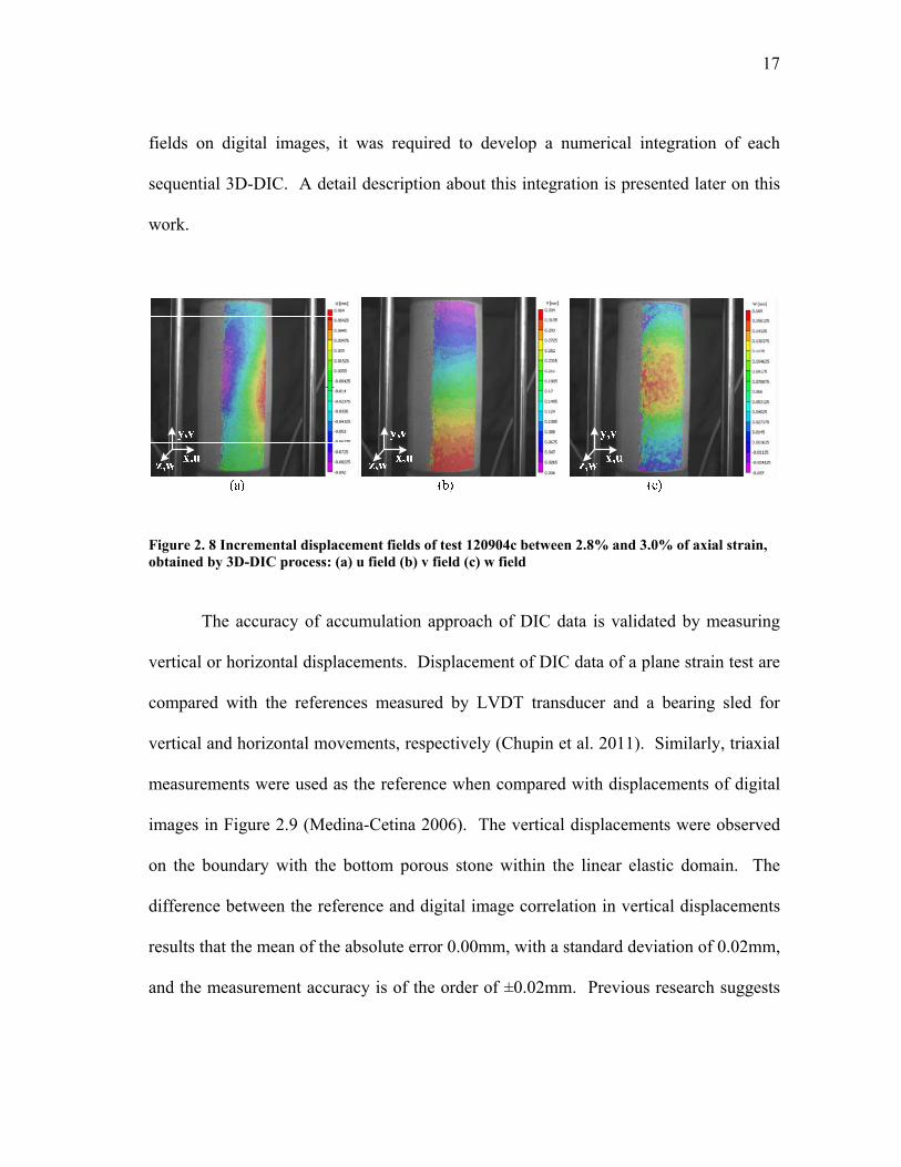
Figure 2. 8 Incremental displacement fields of test 120904c between 2.8% and 3.0% of axial strain, obtained by 3D-DIC process: (a) u field (b) v field (c) w field
The accuracy of accumulation approach of DIC data is validated by measuring
vertical or horizontal displacements. Displacement of DIC data of a plane strain test are
compared with the references measured by LVDT transducer and a bearing sled for
vertical and horizontal movements, respectively (Chupin et al. 2011). Similarly, triaxial
measurements were used as the reference when compared with displacements of digital
images in Figure 2.9 (Medina-Cetina 2006). The vertical displacements were observed
on the boundary with the bottom porous stone within the linear elastic domain. The
difference between the reference and digital image correlation in vertical displacements
results that the mean of the absolute error 0.00mm, with a standard deviation of 0.02mm,
and the measurement accuracy is of the order of ±0.02mm. Previous research suggests

18
that the accuracy of the horizontal and out-of-plane displacements should be of the same
order as the vertical displacements (Sutton et al. 2000).
Figure 2. 9 Accuracy analysis: (a) comparison of displacement measurements between triaxial test system and VIC-3D (b) absolute frequency histogram of absolute error of displacement measurements between triaxial test system and VIC-3D (Medina-Cetina 2006)
2.2.2 Qualitative Assessment of Localization Effects
Shear band observations in laboratory tests have been reported by several authors
(Desrues 1996; Desrues and Viggiani 2004; Rechenmacher 2006). Most of these
investigations were obtained from specifically designed plane strain biaxial tests that are
convenient to study strain localization. In a number of cases, it is known that failure
surfaces take place along pre-existing discontinuities or the loss of homogeneity by the
test execution and preparation. Medina-Cetina (2006) conducted a series of compression
tests on triaxial sand specimens, with a 3D digital imaging system in order to detect and
characterize similar localized effects. Different patterns can be identified for the triaxial
axisymmetric tests, demonstrating the presence of a set of patterns, including both

19
bulging and shearing modes. Their variations are hypothesized to be caused by material
heterogeneity. Another difference with 2D investigations is that the cylindrical samples
have a curved surface and no designated discontinuities. These features make it difficult
to identify the characteristics of a captured area before the sample reaches failure.
The deformed sample photos and corresponding incremental displacement fields
between 11.8% and 12% of axial strain, in the x, y, and z directions captured by VIC-3D
are presented in Figure 2.10 except for the test 120704b. The test 120704b (no.17) ends
at 10% of axial strain, thus its photo and corresponding incremental displacement fields
are estimated at 10% of axial strain (Figure 2.10). The numbers on the photos indicates
the number of the test as mentioned in Table 2.1.
From these images, it is observed that a shearing mode consisting of two shear
bands that cross each other and form a ‘v’ shape was found in thirteen tests. A bulging
mode that constitutes a clear separation of the bottom segment appearing at the upper
segment, expanding in the radial direction was observed in twelve tests. The defined
section between the upper and bottom segments was made by development of shear
bands and the crust of the upper segment tending slide along the shear failure surface.
The layered specimen (no.18) showed a bulging mode on the loose upper segment
indicating an exacerbated compressing behavior when compared with the other results,
but no significant bulging was observed for the dense lower segment. The loose
specimen (no.25) showed localization in terms of axial strain, but no shear bands.

20
Figure 2. 10 Digital image and corresponding incremental displacement fields at 12% of axial strain (a) photo image (b) u field (c) v field (d) w field

21
Figure 2. 10 continued

22
Figure 2. 10 continued

23
Figure 2. 10 continued

24
Figure 2. 10 continued

25
3. 3D DIGITAL IMAGE TRANSFORMATIONS AND INTERPOLATION
3.1 Digital Image Corrections
A 3D-DIC system suffers from the accumulation of inherent error sources such
as cross-camera matching, camera calibration, multiple correlation runs and triangulation
when integrating segments of the displacement fields (Lava et al. 2011; Sutton et al.
2008). The image data is obtained from VIC-3D, which has already considered
corrections for data alignment included in the calibration procedure. From the
calibration images, various system parameters, including camera-based parameters such
as focal length, image center, lens distortion and the relative orientation of the two
cameras in space are computed. Still the plotted shape of the 3D image data on the
Cartesian coordinate system seems to be slightly inclined, which was corroborated by
analyzing the coefficients of the hyperplane equation fitted to the coordinates of the
cloud of data points at the undeformed stage. The best fit plane is found by regression of
all data points and it is very sensitive to the number, a shape and a placement of the
collected image data. To correct for these deviations, a 3D geometric rotation and
translation was conducted with the aim of starting the cumulative analysis of
deformations with the best spatial data reference possible. A 3D geometrical
transformation procedure includes the following steps: (1) the coefficients of an equation
of a best fit plane are computed by regression of all data points, (2) the initial data points
are rotated with the angles calculated from the relationship between a normal vector of a
best fit plane and the y- and z-axes, (3) after rotations, the transformed data points are

26
translated in the y- and z-directions for imposing the data points into the physical
coordinate system.
3.2 Assessment of the Trend Fitting Plane
The selected coordinate system introduced in VIC-3D is configured by a best fit
plane. The best fit plane method imposes a best fit plane on the image data is used to
calculate the transformation of data. In the case when a best fit plane is adopted, the
origin of the best fit plane is located in the middle of the sample height in the x-y plane
and inside of the sample in the z-direction, and the depth of the origin may vary in the z-
direction due to the position of the two cameras. Thus, the physical coordinate system of
a sample is determined to be different from the selected coordinate system of the
analyzed image data. However, the image data points follow a best fit plane, so by
controlling the best fit plane, 3D geometrical transformations can be conducted.
Since it was not possible to retrieve the VIC-3D equation of the best fit plane,
this was found by regression of all the displacement data points. Exported data after
digital image correlation analysis included coordinates of data points and the incremental
displacements in the x-, y-, and z-directions with respect to the reference image.
Coefficients of the trend fitting plane were computed by the code shown in Figure 3.1.
The fitting plane had the form of z=ax+by+c, where a, b, and c are regression-type
coefficients. For example, an equation of a fitting plane for the test 120904c was
z=0.00266x-0.00003y+0.00000.

27
%<Part 1. Geometrical transformations>%%%%%%%%%%%%%%%%%%%%%%%%%%%%%%
clear all fno1='Z40C_120904c-004';%change file name
fnam1=[fno1 '_0.csv'];
A=xlsread(fnam1);
A=A(~any(isnan(A),2),:);%remove NaN rows A(A(:,1)==A(1,1),:)=[];%filter a repeated node
A=[A(:,1) A(:,2) A(:,3) A(:,7) A(:,8) A(:,9)];%save X,Y,Z,U,V,W %a fitting plane%---------------------------------------------------- const=ones(length(A),1);
coeff=[A(:,1) A(:,2) const]\A(:,3);%z=coeff(1)*x+coeff(2)*y+coeff(3)
Figure 3. 1 Code for finding an equation of a fitting plane
3.3 3D Geometrical Transformations
3.3.1 Rotation Analysis
A 3D geometrical transformation is a way to modify the current coordinates by
translation, scaling, reflection, shearing, or rotation by the use of a matrix and vector
systems. In this study, rotation and translation were used to improve the selected
coordinate system.
The best fit plane obtained by regression of all data points was found to be not
parallel to the x-y plane, and slightly inclined, because of the non-uniform distribution of
data points generated after the 3D-DIC. In order to straighten the fitting plane to the x-y
plane, data points must be rotated. The rotation angles are computed by the relationship
between the normal vector of a fitting plane and the y- or z-axes. The normal vector, n,

28
of a fitting plane is induced from the coefficients of a fitting plane with a general form
(a,b,-1). Note that a vector forms a right-handed system. A cross product of n and a unit
vector of the z-direction is a vector, m.
i j k
=(0,0,1)×(a,b,-1)= 0 0 1 =-bi+aj=(-b,a,0)
a b -1
m
The angle, φ, between a vector m and a unit vector in the y-direction is given by
the following formula.
-1 -1
2 2 2 2
(-b,a,0)•(0,1,0) aφ=cos =cos
a +b a +b
The angle, θ, between a vector n and a unit vector of the negative z-direction is
given by the following formula.
-1 -1
2 2 2 2
(a,b,-1)•(0,0,-1) 1θ=cos =cos
a +b +1 a +b +1
The plane should be adjusted to be parallel to the x-y plane, thus the normal
vector, n, rotates on the z-axis with an φ angle and becomes the transformed vector n’.
The vector, n’, rotates on y-axis with a negative θ angle and becomes a vector n”. Data
points follow a fitting plane with rotations of the normal vector, n, so that it straightens
up with a fitting plane that is parallel to x-y plane. Figure 3.2 shows the rotation steps
and normal vectors at each step in space and Figure 3.3 illustrates the rotation processes
of data points. The transformation process in matrix form is coded based on the 3D
rotation description of Foley et al. (1996), and the code is shown in Figure 3.4.

29
Figure 3. 2 3D geometrical transformation process (a) normal vectors in space (b) rotation process
Figure 3. 3 Schematic view of 3D transformations: rotation
%Rotation on the z-axis
psi=acos(coeff(1)/sqrt((coeff(1)^2)+(coeff(2)^2)));
if coeff(2)<0%if coeff a>0,b<0, use(psi), a>0,b>0, use(-psi) for Rz
Rz=[cos(psi) -sin(psi) 0 0 0 0;
sin(psi) cos(psi) 0 0 0 0;
0 0 1 0 0 0
0 0 0 cos(psi) -sin(psi) 0
0 0 0 sin(psi) cos(psi) 0
0 0 0 0 0 1];
Figure 3. 4 Code for rotation process

30
else
Rz=[cos(-psi) -sin(-psi) 0 0 0 0; sin(-psi) cos(-psi) 0 0 0 0;
0 0 1 0 0 0
0 0 0 cos(-psi) -sin(-psi) 0
0 0 0 sin(-psi) cos(-psi) 0 0 0 0 0 0 1];
end B=Rz*A'; %Rotation on the y-axis
theta=acos(1/sqrt((coeff(1)^2)+(coeff(2)^2)+1^2));
Ry=[cos(-theta) 0 -sin(-theta) 0 0 0;
0 1 0 0 0 0; sin(-theta) 0 cos(-theta) 0 0 0
0 0 0 cos(-theta) 0 -sin(-theta);
0 0 0 0 1 0; 0 0 0 sin(-theta) 0 cos(-theta)];
C=Ry*B; C=C';
Figure 3. 4 continued
To illustrate the proposed post-processing scheme, a simple case with 10
coordinate points is taken from the boundary of test 120904b. Results of the fitting
plane and rotation of data points are shown in Figure 3.5. Blue data points and an
inclined plane indicate the state before the rotations and red data points and a horizontal
plane in the x-z view show the position after rotations. In the same way, this rotation
process is applied to the test 120904b and the results are presented in Figure 3.6. Before
rotations, the equation of the plane is z=0.00433x+0.00001y+0.00000 and after the

31
rotations, the equation of the plane of transformed data points changes to
z=0.00011x+0.00000y+0.00000. This means that a fitting plane is changed to be
parallel to the x-y plane and the coefficients of the plane, a and b, become closer to zero,
indicating a proper coordinate transformation.
Figure 3. 5 Geometrical transformation of 10 data points (a) xyz view (b) x-z view
Figure 3. 6 Geometrical transformation of test 120904b (a) before rotations (b) after rotations

32
3.3.2 Translation Analysis
After the 3D-DIC pre- and post- processing is completed, the origin of the data
points is set up inside and mid-height of a sample. In the physical coordinate system, the
bottom of a specimen is assumed to be the x-z plane with y=0 and the center axis of a
sample coincides with the y-axis, which means that all data points must move up (y-
direction) and forward (z-direction) to impose displacement fields on a finite element
model. The data points are translated to the new coordinate system by adding translation
amounts to the current coordinates of the points. All data points are moved by ‘yb’ and
‘z_add’. ‘yb’ is the distance in the y-direction from the bottom to the center and it is
decided by reading of bottom coordinates from the first digital image of the undeformed
state. ‘z_add’ is the distance in the z-direction from the center of a specimen to the best
fit plane and it is calculated by subtracting ‘z_avg’ from the measured radius presented
in Table 2.1. ‘z_avg is an averaged value, taken from the data points with the threshold
between -0.02 mm and 0.02 mm of x because ’z_avg’ is theoretically the z value when x
is equal to zero, but real data is scarcely at the position of exact x=0. Figure 3.7 and 3.8
illustrate how to find ‘yb’ and ’z_add’ and the translation process. Code in Figure 3.9
explains how to compute ‘z_add’ and shows the translation matrix.

33
Figure 3. 7 Translation on y- and z- directions (a) y-direction translation (b) z-direction translation
Figure 3. 8 Schematic view of 3D transformations: translation
%Translation y- and z- directions ------------------------------------ %yb from 'Reference_coordinates.xls': check minY, maxY, and height
yb=-78.6352;
%radius from 'DIA_SummaryAnlayses.xls' Data Summary sheet radius=35.55;
row=find(-0.02<=C(:,1)&C(:,1)<=0.02);%threshold -0.02<=x<=0.02 S=C(row,:);
z_ave=mean(S(:,3));
z_add=radius-z_ave; Tyz=repmat([0 -yb z_add 0 0 0],length(A),1); D=C+Tyz;
Figure 3. 9 Code for translation in y- and z-directions

34
Figure 3.10 is an example of a completed translation. The range of y varies
between 0 to 158cm and the maximum z value corresponds to the radius of the test
120904b.
Figure 3. 10 Result of test 120904b after translation on y- and z- directions
3.3.3 Trend Fitting Plane Coefficients and Rotation Analysis
Figure 3.11 shows a snapshot image of the raw coordinate’s data, and the fitting
plane plots in the x-z plane for test 120904c. It was observed that in general, plots
before and after rotations did not show a significant difference. To investigate the
effects of rotation angles, plane coefficients and rotation angles from each fitting plane,
results of the coordinate transformation are presented in Table 3.1 and Figure 3.12.
35
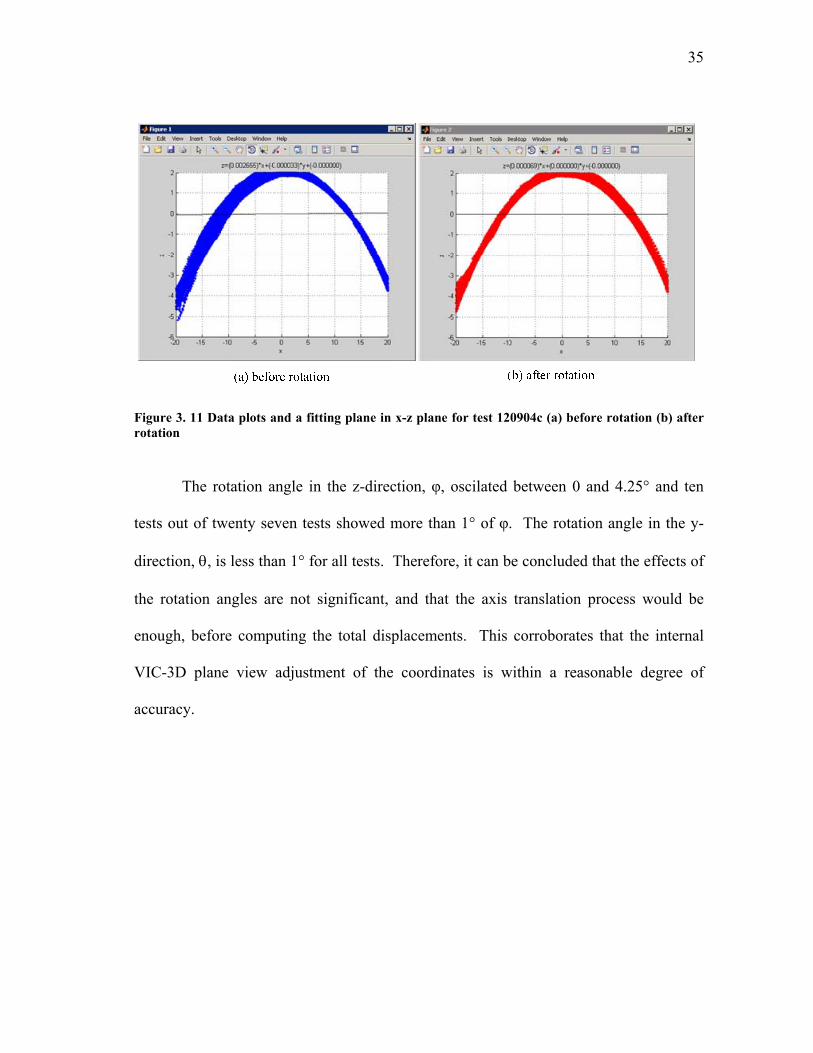
Figure 3. 11 Data plots and a fitting plane in x-z plane for test 120904c (a) before rotation (b) after rotation
The rotation angle in the z-direction, φ, oscilated between 0 and 4.25° and ten
tests out of twenty seven tests showed more than 1° of φ. The rotation angle in the y-
direction, , is less than 1° for all tests. Therefore, it can be concluded that the effects of
the rotation angles are not significant, and that the axis translation process would be
enough, before computing the total displacements. This corroborates that the internal
VIC-3D plane view adjustment of the coordinates is within a reasonable degree of
accuracy.

36
Table 3. 1 Plane coefficients and rotation angle analysis (plane equation: z=ax+bx+c)
Case Plane Coefficients Angle (deg)
No. Test Name a b c φ
1 092903b 0.00623 -0.00008 0 0.76292 0.35715
2 093003b -0.00594 -0.00012 -0.00002 1.15811 0.34017
3 100103a -0.00188 -0.00010 0.00003 2.91701 0.10809
4 100103b -0.00682 -0.00026 -0.00073 2.20098 0.39087
5 100103c -0.00643 -0.00007 0 0.58772 0.36866
6 100103d -0.00914 -0.00016 0 0.98398 0.52380
7 100203a -0.00887 -0.00012 0 0.78146 0.50830
8 100203b -0.00730 -0.00018 0 1.39622 0.41855
9 100303b -0.00449 0.00000 0 0.00000 0.25697
10 101104a -0.01320 -0.00024 0 1.05866 0.75662
11 101204a -0.01627 0.00013 0 0.44021 0.93209
12 120604a 0.00698 -0.00006 0 0.50049 0.40011
13 120604b 0.00652 -0.00001 0 0.05273 0.37356
14 120604c 0.00759 -0.00007 0 0.49821 0.43488
15 120604d 0.00765 0.00005 0 0.38222 0.43803
16 120704a 0.00427 -0.00006 0 0.84489 0.24479
17 120704b 0.00590 -0.00010 0 0.92279 0.33797
18 120704c 0.00541 -0.00010 0 1.02681 0.31013
19 120904a 0.00561 -0.00006 0 0.59245 0.32139
20 120904b 0.00433 -0.00001 0 0.13229 0.24815
21 120904c 0.00266 -0.00003 0 0.71211 0.15213
22 120904d 0.00267 0.00000 0 0.08584 0.15298

37
Table 3. 2 continued
Case Plane Coefficients Angle (deg)
No. Test Name a b c φ
23 120904e -0.00326 0.00017 0.04187 3.05522 0.18705
24 121304a 0.00230 -0.00014 0 3.56545 0.13175
25 121304b 0.00405 -0.00013 0 1.84031 0.23194
26 121304c 0.00188 -0.00014 0 4.25209 0.10819
27 121304d 0.00254 -0.00001 0 0.24833 0.14542
Figure 3. 12 Rotation angle analysis (a) rotation angles of each test (b) frequency histogram of rotation angle
3.4 Interpolation of Image Data
3.4.1 Interpolation and Extrapolation for Cumulative Displacement Fields
Displacements are computed by comparing the position of a data point between
the reference image and consecutive images. However, if a data point is out of the area

38
which is available to capture data points by the cameras, displacements are no longer
acquired. For that reason, the 3D-DIC system updated the reference images for every 4th
image, and consequently the coordinates of each sequence of image deformation do not
correspond to each other (i.e. every segment of analysis is independent of each other).
Interpolation and extrapolation of reference image data is therefore the key to elicit
cumulative displacement fields with respect to the first reference image (undeformed
state at zero strain).
Figure 3.13 illustrates the interpolation and extrapolation flow chart analysis as
applied from image no.000 to image no.008, which corresponds to 0.4% of axial strain.
The reference image for the no.000-004 image set is image no.000, but for the no.004-
008 image set, the reference image is now image no.004. The reference image of the
no.004-008 image set is extrapolated on designated grid points. Extrapolated
displacements on this grid required to be updated from the previous node position. The
displacement from the initial position of nodes of image no.000 to the final position of
no.008 becomes the cumulative displacement of image no.008. Figure 3.14 shows
actual image data movements by the interpolation and extrapolation in the data
subsample corresponds to the center of the specimen, close to x=0, y=80mm.
Cumulative total displacement fields of the undeformed state (image no.000) and
deformed state (image no.008) at 0.4% of axial strain are shown in Figure 3.15.

39
Figure 3. 13 Scheme of interpolation and extrapolation
Figure 3. 14 Interpolation and extrapolation between image no.000 and no.008 (0.4% of axial strain)

40
Figure 3. 15 Total displacement fields of test 120904c (a) undeformed state (b) deformed state at 0.4% of axial strain
3.4.2 Interpolation for Ccorrection of Incorrect Image Data
As illustrated in Figure 2.10, light reflection causes missing data points or
incorrect assessment of displacement values because the 3D digital image system could
not recognize pixels in that area, even within a short deformation range. Also, an
excessive gap produced between bulging zone and a bottom block by shearing plane
brings incorrect w displacement fields. During a compression loading, some sand
particles stuck between a membrane and other soil particles show no movement in the
vertical direction which could contribute to incorrect data points. Figure 3.16 is an
example where it is required to solve a light reflection problem by an interpolation
method using contiguous data points to the missing data zone. Another example of a
similar problem is presented in Figure 3.17, where a gap occurred by shearing and radial
displacement plots generated a poor displacement recognition by VIC-3D. In cases like
these, raw data points are replaced with interpolated data points, conditioned by

41
contiguous data points near the gap. Improved displacement field assessment is
presented on Figure 3.16 (c) and 3.17 (c) respectively.
Figure 3. 16 Correction of light reflection problem for test 120704c
Figure 3. 17 Correction of incorrect data generated by shearing plane for test 121304d
3.5 Cumulative Displacement Fields
Cumulative radial and vertical displacement fields at 0.2%, 3.6%, 7% and 12%
of axial strain after the 3D-DIC analyses are presented in Figure 3.18 and 3.19
respectively. Figure 3.18 illustrates the horizontal, vertical, and out-of-plane

42
displacement fields (u, v, and w fields) in Cartesian coordinates. Horizontal
displacement fields show a developing persistent shear band clearly from 3.6% of axial
strain. Vertical displacement fields at the bottom of the specimen correspond to global
displacement, which follows displacement loading rate with 0.2% of axial strain/min.
The out-of-plane displacement fields show a bulging zone that becomes evident after 3.6%
of axial strain.
Radial displacement fields mainly represent the bulging effect of the specimen,
which shows higher displacement values around the mid height of the sample. Notice
that the vertical displacements at the bottom of the specimen correspond to the global
displacement that follows the strain rate during shearing. After peak, Figure 3.19 (d)
shows a clear distinction of displacement fields between the bottom segment and the rest
of the specimen. This can be interpreted as a separated portion of the sample moving as
a block.

43
Figure 3.20 (a) shows the average of the radial displacement across the same
heights over the surface of the sample. This is symmetric with respect to the midpoint of
the boundary at strain levels between 0.2% and 3.6% of axial strain, but definitely not
after 7% of axial strain. This observation is expected, due to the shear plane that
developed in the specimen after the peak stress. The shear band seen in Figure 3.19 (d)
can also be seen by observing the displacement fields shown in Figure 3.19 (d). Unlike
the displacements in the radial direction, the vertical displacements are distributed
linearly at 0.2% and 3.6% of axial strain, but they become non-homogeneous after the
peak. This change in the distribution confirms the presence of a shear plane in the
sample. Based on the observed results, the bottom segment of the specimen is separated
from the bulging surface of the specimen by shearing, and then it moves independently
as a single block.

44
Figure 3. 18 Cumulative displacement fields of test 120904c in Cartesian coordinate system at 0.2%, 3.6%, 7%, and 12% of axial strain: (a) horizontal (u) displacement field (b) vertical (v) displacement field (c) out-of-plane (w) displacement field

45
Figure 3. 19 Cumulative displacement fields of test 120904c in cylindrical coordinate system at 0.2%, 3.6%, 7%, and 12% of axial strain: (a) radial displacement field (b) tangential displacement field (c) axial displacement field

46
Figure 3. 20 Averaged displacements of test 120904c (a) radial displacement (b) vertical displacement
Cylindrical displacements, radial and tangential displacements, are computed
from standard VIC-3D u, v, and w displacement fields in Cartesian coordinates. Radial
and tangential displacements are calculated by the angles determined from the
relationship between x and z or dx (i.e. u) and dz (i.e. w) as well as u and w
displacements. A graphical explanation about the calculation of cylindrical
displacements is presented in Figure 3.21.

47
-1 -1
-1
-1
z dztan if x>0 tan
x dx
ztan +π if x<0 and z 0
x
ztan -π if x<0 and z 0θ = , dθ = x
π if x=0 and z>0
2π
- if x=0 and z<020 if x=0 and z=0
-1
-1
if dx>0
dztan +π if dx<0 and dz 0
dx
dztan -π if dx<0 and dz 0
dx
π if dx=0 and dz>0
2π
- if dx=0 and dz<020 if dx=0 and dz=0
2 2i i i i idr = dx +dz × cos(θ -dθ ) : radial displacement
2 2i i i i idt = dx +dz × sin(θ -dθ ) : tangential displacement
2 2i idx +dz
2 2i i ir = x +z
Figure 3. 21 Conversion between Cartesian and cylindrical coordinate systems

48
3.6 Cumulative Strain Fields
The cumulative strain fields are derived from the cumulative displacements fields
in the same way as computing the cumulative displacements using strain-displacement
relationships. Assuming small or infinitesimal strains, shear strain components for three
dimensional cases (Desai and Siriwardane 1984; Iskander 2010) are expressed as
x 11
uε =ε =
x
y 22
vε =ε =
y
xy 12
1 u vε =ε = +
2 y x
Above, represents a local strain field, with the x-axis direction, 11, and the y-
axis direction, 22. Horizontal and vertical displacement fields in plane are represented
with u and v. Shear bands are coaxially crossed from the peak stress, which can be
observed at 7% and 12% of axial strain in Figure 3.22.

49
a 0.2%
(b) 22 field (c) 12 field(a) 11 field
a 3.6%
a 7.0%
a 12.0%
Figure 3. 22 Cumulative strain fields of test 120904c at 0.2%, 3.6%, 7%, and 12% of axial strain: (a) 11 field (b) 22 field (c) 12 field

50
3.7 Volumetric Strain
Due to the lack of volumetric strain measurements (Plexiglass cell was removed
to avoid image distortion), a method is proposed based on the representation of the
volume specimen as a sum of a series of stacked disks. To determine the volume of the
specimen making this assumption, it is required to know the diameter and height of each
individual disk. The height of each disk was assumed to be a uniform height of 1 mm,
whereas the diameter of each disk was obtained from the initial specimen profile,
assumed as the average of the actual radius measured on the area of interest for each
‘layer’. This approach has been used previously with a circular disk model to estimate
the volume from a digitized image (Macari et al. 1997). Results from this technique
showed a qualitative good agreement to conventional volumetric strain measurements
obtained in wet conditions. This procedure was selected as an alternative method to
measure the volume changes of dry sand specimens.
In order to compute the volume change of a specimen and volumetric strain
according to the axial strain, the cylindrical volume calculation method was adopted.
After transformation and interpolation of the coordinate data points, it is observed that
these are not uniformly distributed on a Cartesian coordinate system. Thus, the data
points and their displacements are redistributed on a material domain grid with each 1
mm space in the x-, y-, and z-directions. A representative radius of the ith layer is
computed by averaging the radius of each data points at the layer. The number of data
and the y (height) range depend on the resolution of the digital image for the
deformation process. Although digital image correlation is capable of showing a wide

51
range of a specimen surface at relatively early stages of loading, unfortunately the
identifiable range decreases from the top platens as the loading progresses. The upper
limit of the height is therefore bounded by 155~160 mm, which is the height of the
samples, if the y-direction data exceeds the height of the sample. Otherwise, if y-
direction data is recorded less than the height, a fixed data point with the measured
height and radius is provided as an upper bound. The lower bound of a specimen is
changing by the bottom platen and is reflected in the collected digital image data, so it
does not need to be modified.
Figure 3. 23 Process for averaging radius and uniformalizing height

52
Once all the new coordinate data points with radius and heights are computed,
the volume of each layer is estimated by the use of a trapezoidal numerical integration
function and then added together. Since all the data points are forced to be located in a 1
mm grid and y-direction lower boundary change is not smooth, it is expected that the
averaged volume with respect to height shows some variation.
H 2π R H 2π H H2 2 2
0 0 0 0 0 0 0
1 1V= r dr dθ dz= R dθ dz= R 2π dz=π R dz
2 2
The local effects captured by the VIC-3D can be averaged with respect to the
height of the specimen as illustrated in Figure 3.24, which presents the averaged radius
profile in a blue line with a standard deviation in a red line, and the number of data
points in a black line. The data points contacting on the top porous stone were lost in the
interpolation and extrapolation process for cumulative displacements. Thus, the average
radius at the top of the specimen is assumed as the initial measured radius of the sample,
and the whole volume of the specimen is computed including the extrapolation of the
missing data with respect to the initial condition.

53
Figure 3. 24 Averaged radius profile for test 120904c at (a) 0.2% of axial strain (b) 3.6% of axial strain (c) 7% of axial strain (d) 12% of axial strain
Figure 3.25 presents the axial strain vs. volumetric strain relationship computed
using the disks’ profile assumption obtained from the radius profile after the VIC-3D
digital image analysis. This example shows how the sample is compressed from the
initial state up to 1.4% of axial strain and then dilates, until it reaches the critical state at
8.8% of axial strain. A calculation code for a sample volume is presented in Figure 3.26.

54
Figure 3. 25 Axial strain vs. volumetric strain curve of test 120904c
%<Part 4. Volume>%%%%%%%%%%%%%%%%%%%%%%%%%%%%%%%%%%%%%%%%%%%%%%%%%%%%%
%height from 'DIA_SummaryAnlayses.xls' Data Summary sheet, use integer
height=159; if yym(length(yym),1)>=height;
row=find(yym(:,1)==height);
vol=pi*trapz(yym(1:row,1),rmint_mean(1:row).^2); vol_add=0;
else yym=[yym;repmat(height,1,size(yym,2))];
rmint=[rmint;radius repmat(nan,1,size(rmint,2)-1)];
rmint_mean=[rmint_mean;radius]; vol=pi*trapz(yym(:,1),rmint_mean.^2);
row=find(yym(:,1)==height); end
Figure 3. 26 Code for volume calculation

55
4. SIMPLE ONE ELEMENT MODEL TEST
4.1 Calibration of Model Parameters
The global stress-strain behavior of the test 120904c specimen captured by the
triaxial testing system is presented in Figure 4.1 (a). This shows the typical behavior of
a dense sand. Meanwhile, the volumetric strain is computed from the 3D-DIC analysis
as explained before, since the specimen was vacuum consolidated. Results from the
computed volumetric strain are presented in Figure 4.1 (b).
The interpretation of the triaxial results makes it possible to represent the dilative
behavior of the sand by using an elasto-plastic model. The elastic and plastic parameters
which can be deduced from the test are: Poisson’s ratio, Young’s modulus, dilation
angle, axial strains at the characteristic state and the plastic limit as shown in Figure 4.1.
The Mohr-Coulomb model parameters are determined by the graphical interpretation of
the triaxial results according to the approach presented by Gay et al. (2003).

56
13846E kPa
1 2
2sin1 sin
peak
crit
1
Figure 4. 1 Global stress-strain behavior of test 120904c (a) stress vs. strain curve (b) axial strain vs. volumetric strain curve
4.2 One Element Model Test Cases
The purpose of performing a one element model analysis is to calibrate the soil
constitutive model based on the global stress-strain measurements. In the case of the one
element model, the local stresses and strains are expected to show small variations,
compared with the global stresses and strains. Under this condition, the results of a
finite element model could be directly compared to the calculation from the constitutive
model, so the material properties and boundary conditions can be easily validated.
A set of analysis including one element model test cases, and its material
properties are presented in Table 4.1. Both One_pk and One_cr tests were compared to
explore the effect of the friction angle, which is obtained at the peak and critical state,
and the One_pk_pp and One_cr_pp tests aimed at modeling sands using an elasto-
perfectly plastic model, i.e. a traditional Mohr-Coulomb model. Test One_pk_step
consists of two loading steps, an initial condition under consolidation and displacement
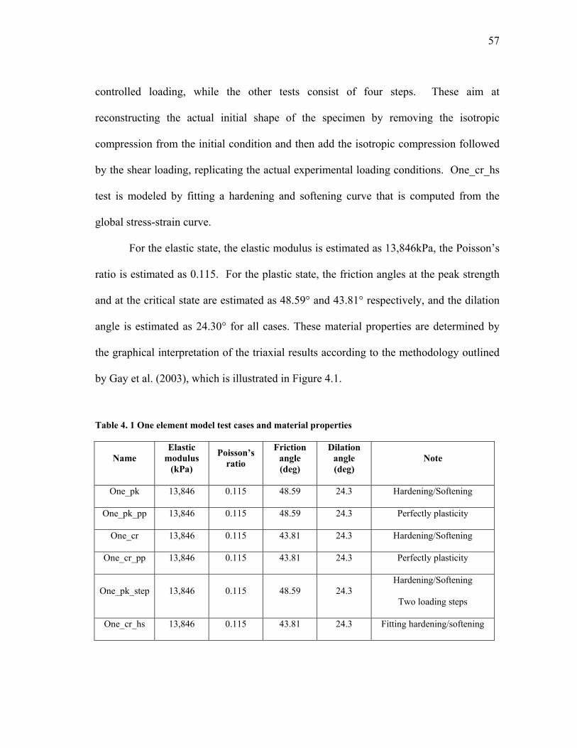
57
controlled loading, while the other tests consist of four steps. These aim at
reconstructing the actual initial shape of the specimen by removing the isotropic
compression from the initial condition and then add the isotropic compression followed
by the shear loading, replicating the actual experimental loading conditions. One_cr_hs
test is modeled by fitting a hardening and softening curve that is computed from the
global stress-strain curve.
For the elastic state, the elastic modulus is estimated as 13,846kPa, the Poisson’s
ratio is estimated as 0.115. For the plastic state, the friction angles at the peak strength
and at the critical state are estimated as 48.59° and 43.81° respectively, and the dilation
angle is estimated as 24.30° for all cases. These material properties are determined by
the graphical interpretation of the triaxial results according to the methodology outlined
by Gay et al. (2003), which is illustrated in Figure 4.1.
Table 4. 1 One element model test cases and material properties
Name Elastic
modulus (kPa)
Poisson’s ratio
Friction angle (deg)
Dilation angle (deg)
Note
One_pk 13,846 0.115 48.59 24.3 Hardening/Softening
One_pk_pp 13,846 0.115 48.59 24.3 Perfectly plasticity
One_cr 13,846 0.115 43.81 24.3 Hardening/Softening
One_cr_pp 13,846 0.115 43.81 24.3 Perfectly plasticity
One_pk_step 13,846 0.115 48.59 24.3 Hardening/Softening
Two loading steps
One_cr_hs 13,846 0.115 43.81 24.3 Fitting hardening/softening

58
4.3 Boundary and Loading Conditions
By taking advantage of the symmetric configuration of a cylindrical specimen, a
2D axisymmetric finite element, 4-node bilinear with reduced integration (CAX4R)
model is adopted. The geometry of the element is 10cm in height and 5cm in radius,
following the height to radius ratio of the experimental sample.
The boundary and loading conditions were set up by referring to the examples
about the consolidation of a triaxial test specimen (Bayoumi 2006; Helwany 2007;
ABAQUS user’s manual 2008). The initial and loading conditions consist of four steps:
step 1 (initial geometry and confining stress), step 2 (release confining stress), step 3 (re-
application of confining stress), and step 4 (shear loading). The stress paths of this
sequence as described on the p-q stresses plane are illustrated in Figure 4.5 (a), while
boundary conditions and stress loading at each step are shown in Figure 4.2. At step 1,
the initial confining pressure is defined through the initial condition option in ABAQUS,
with boundaries restrained so that the initial geometry of the specimen can be replicated.
Step 2 simulates the actual initial state with a ‘zero’ stress condition by applying a
tensile isotropic stress to the element. In this step, the restraints along the element
boundaries are removed except for the bottom surface, letting the specimen deform to its
true initial geometry. Assuming the element after step 2 is in the actual initial condition
of a triaxial test, step 3 and step 4 simulate the actual confining and shear loadings. The
confining pressure is applied on the element in step 3. From this experiment, it is
observed that the boundary conditions for step 3 are the same as step 2. However, the
stresses and displacements after step 3 indicate almost the same values as the results of

59
step 1. This means that the modeling of the actual initial state (step 2) has no effect on
the initial geometry of the specimen. At step 4, only the top boundary is restrained and
the bottom boundary is controlled by uniform displacement as a loading. As the element
is compressed by the displacement control, both the mean and deviatoric stresses are
increased. The mean stress and vertical displacement contours in Figure 4.3 and 4.4
prove that the boundary and loading conditions of all the procedures are set up correctly.
Figure 4. 2 Applied loading steps on the one element model
Figure 4. 3 Mean stress contour at different loading steps

60
Figure 4. 4 Vertical displacement contour at different loading steps
In order to examine the loading phases, test One_pk with a full loading sequence
(step 1 to step 4), and test One_pk_step with step 1 (initial condition) and step 2
(displacement loading) are compared in Figure 4.5. The stress path during loading is the
same for both One_pk and One_pk_step tests and an observed difference is whether a
model can simulate the real initial state with zero stress. An effect on the element by
additional steps to simulate the process from the initial state to confinement is not
expected to provide any additional stress or strain, which proves that step 2 and step 3
(release stress and confinement) can be neglected to provide an economical analysis on a
larger finite element model.

61
Figure 4. 5 Stress paths in p-q plane (a) four loading steps condition of test One_ pk (b) two loading steps condition of test One_pk_step
In a loading step of a nonlinear finite element analysis, the step is divided into
increments and iterate as much as necessary. Since increments that correspond to the
force or displacement increments applied in nodes control the numerical solutions, it is
important to obtain accurate result in the behavior of materials and to avoid iteration
errors in solution process (Zienkiewicz and Taylor 2000; Sloan et al. 2001). In this
study, the maximum increment was restricted to 1.2% of axial strain and the tolerance is
0.06% of axial strain with automatic incrementation that allows the flexible increment
size for an effective analysis. In addition, Newton’s method with unsymmetric stiffness
matrix storage was used to solve this nonlinear problem. Some cases can be solved with
the extra iteration by a symmetric matrix, but this problem with Coulomb friction was
needed to use “unsymm” option to improve the convergence in ABAQUS. Since a
friction coefficient was modified to simulate a hardening and softening behavior of

62
dense sands, it would not be able to complete the analysis without introducing the
unsymmetric matrix storage.
4.4 Stress and Strain Behavior
From the experimental results it is observed that at the end of the tests the shear
stress condition represents the critical state, where the soil continues to deform at a
constant stress ratio q/p’ and constant specific volume. The critical state line (CSL) is
defined by the following equation, q=Mp’, where M is the critical state parameter related
to the friction angle at critical state, crit (Schofield and Wroth 1968; Atkinson and
Bransby 1978; Powrie 1997).
For an elasto-perfectly plastic material, the selected friction angle for the finite
element model defines the slope of the yield surface by the critical state parameter, M
that is related to the critical state as shown in Figure 4.6. Thus by taking the friction
angle at the critical state, hardening and softening straining can be controlled by varying
the yield surface.

63
Figure 4. 6 Comparison of stress-strain behavior of an elasto-perfectly plastic models with different friction angles at peak and critical state
An elasto-plastic models with hardening and softening laws (test One_pk) and an
elasto-perfectly plastic model (test One_pk_pp) are compared in Figure 4.7. For the
elasto-perfectly plastic model, the friction angles at both the critical state and peak state
are the same (crit=peak). When the stress path reaches the critical state, where the soil
response is perfectly plastic, a limit state is attained. If a model is used as a failure
surface, the material exhibits an unlimited flow when the stress reaches yield. This is a
perfect plasticity behavior. Since the model is also provided with isotopic hardening and
softening, plastic flow causes the yield surface to change size uniformly with respect to
all stress directions. This hardening and softening laws are useful for cases involving
plastic straining, so the evolution of the yield surface with plastic deformation is
described in terms of stresses as shown in Figure 4.7 (b).

64
6sin
3 sin
qM
p
Figure 4. 7 Comparison of stress-strain behavior between an elasto-perfectly plasticity model and an elasto-plasticity model
For the elasto-plastic model with the hardening and softening laws, the stress
path jumps the critical state line because of hardening straining in Figure 4.7. The
hardening and softening curve is defined as a relationship between the equivalent plastic
strain (PEEQ) and cohesion yield stress (c) in ABAQUS. The cohesion yield stress must
be greater than zero, in the case of an elasto-perfectly plastic material the cohesion yield
stress is given as a very small number, for example, 10-6. This means that if the friction
angle at the peak state is used for the finite element analysis, the deviatoric stress never
reach the limit at the critical state. This means that the friction angle at critical state
should be applied as an input parameter for the soil constitutive model, and the peak
stress of the soil would be controlled by the cohesion yield stress of the
hardening/softening curve.
In the analysis, soil materials conformed to the Mohr-Coulomb yield criterion,
which has already provided by ABAQUS, together with implementation of the

65
hardening/softening law. Figure 4.8 illustrates the Mohr-Coulomb yield surface in
principal stress space and in the p-Rmcq stress plane as coded in ABAQUS. The yield
surface touches the corner of hexagon at the Lode angle =/3 (triaxial compression).
Various methods for smoothing the corners in Mohr-Coulomb yield functions have been
discussed. Sloan and Booker (1986) modified yield functions for round vertices in the
range 25° to 29° of Lode angle at which the transition occurs. Abbo (1997) used a
hyperbolic approximation of the surface that removes all gradient singularities from the
Mohr-Coulomb yield function. Zienkiewicz and Taylor (2000) modified the yield
function that becomes an overall rounded surface. Similarly, the Mohr-Coulomb
function defined in ABAQUS is modified to the elliptic function using a parameter that
describes the out-of-roundedness in terms of stresses. This modification allows the
convergence of numerical computation at corners in the yield surfaces.
The friction angle () is defined as the slope of the Mohr-Coulomb yield surface
in the p-Rmcq stress plane in ABAQUS (Figure 4.8). The Mohr-Coulomb yield criterion
is defined as mcF=R q-ptan -c=0 , where is the friction angle and c represents the
evolution of the cohesion of the material in the form of isotropic hardening or softening
and a function of plε (PEEQ) that is an equivalent plastic strain. Rmc is a function of the
deviatoric polar angle () and friction angle () and defined as
mc
1 π 1 πR (θ, )= sin θ+ + cos θ+ tan
3 3 33cos
where the deviatoric polar angle () defined as

66
3
3D3/22D
r 3 3Jcos(3θ)= =
q 2J
If the deviatoric polar angle is equal to /3, Rmc becomes a function of only the
friction angle. The Mises equivalent stress (deviatoric stress), q, and a function of the
third invariant of deviator stress, r, are define as follows.
2D
3q= (S:S)= 3J
2
1
33
3D
9 27r= S×S:S r = J
2 2
Figure 4. 8 Mohr-Coulomb yield surface in meridional and deviatoric planes (ABAQUS user’s manual 2008)

67
4.5 Hardening and Softening Analysis
4.5.1 Stress and Strain Relationship in the Hardening and Softening Curve
As output of finite element analysis for the one element model, stress and strain
components in vertical (notated as direction 1) and radial (notated as direction 2) are
obtained, and these components are compared with the components that are computed by
the equations of linear elasticity and the yield function and potential function of the
Mohr-Coulomb model. The vertical total strain component ( 11ε ) is defined by the
amount of displacement that applied as a loading and the deviatoric stress ( dσ ) is
captured as a reaction force on the top surface of an element. The elastic and plastic
strain components ( e11ε , e
22ε , p11ε and p
22ε ) are calculated as follows.
e11 d
e e22 11
p el11 11 11
p p p22 11
ε =σ /E
ε =ε ×-ν
ε =ε -ε
ε =ε ×ν
where ν is the Poisson’s ratio and pν is a plastic component of the Poisson’s ratio,
which is determined by plastic strain components. Dean and Crocker (2001) reported
the plastic component of the Poisson’s ratio determined under uniaxial tension for the
linear Drucker-Prager model and this concept is modified to follow the Mohr-Coulomb
model criterion.

68
The general flow rule is defined as
p Qdε =λ
σ
where Q is potential function as expressed 2 2mw0
Q= ( c tanψ) +(R q) -ptanψ
where is a parameter for the meridional eccentricity, 0
c is an initial cohesion yield
stress, ψ is the dilation angle, and Rmw is as follows.
2 2 2
mw mc2 2 2 2
4(1-e )cos θ+(2e-1) πR (θ,e)= R ,
32(1-e )cosθ+(2e-1) 4(1-e )cos θ+5e -4e
where e is a parameter for the deviatoric eccentricity and by default, it can be defined as
a function of the friction angle.
3-sine=
3+sin
mc
π 3-sinR , =
3 6cos
If the deviatoric polar angle () is equal to /3, Rmw becomes a function of the
friction angle.
mw mc
π π 3-sinR ( ,e)=R , =
3 3 6cos
Therefore, using the flow rule and the definition of a plastic component of the
Poisson’s ratio, pν is defined as a function of the friction angle and the dilation angle.
p mwp 22 22
p11
mw11
Q 3-sin 22 + tanψR + tanψdε σ1 1 1 16cos 33ν = × = × = × = ×Q 1 3-sin 1dε 2 2 2 2-R + tanψ - + tanψσ 3 6cos 3
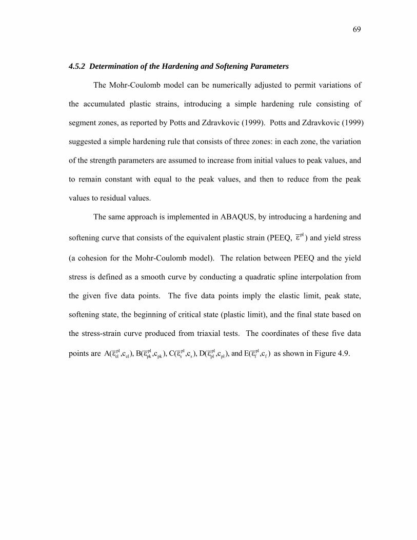
69
4.5.2 Determination of the Hardening and Softening Parameters
The Mohr-Coulomb model can be numerically adjusted to permit variations of
the accumulated plastic strains, introducing a simple hardening rule consisting of
segment zones, as reported by Potts and Zdravkovic (1999). Potts and Zdravkovic (1999)
suggested a simple hardening rule that consists of three zones: in each zone, the variation
of the strength parameters are assumed to increase from initial values to peak values, and
to remain constant with equal to the peak values, and then to reduce from the peak
values to residual values.
The same approach is implemented in ABAQUS, by introducing a hardening and
softening curve that consists of the equivalent plastic strain (PEEQ, plε ) and yield stress
(a cohesion for the Mohr-Coulomb model). The relation between PEEQ and the yield
stress is defined as a smooth curve by conducting a quadratic spline interpolation from
the given five data points. The five data points imply the elastic limit, peak state,
softening state, the beginning of critical state (plastic limit), and the final state based on
the stress-strain curve produced from triaxial tests. The coordinates of these five data
points are pl pl pl pl plel el pk pk s s pl pl f fA(ε ,c ), B(ε ,c ), C(ε ,c ), D(ε ,c ), and E(ε ,c ) as shown in Figure 4.9.

70
Yie
ld s
tres
s
plel elA(ε ,c )
plpk pkB(ε ,c )
pls sC(ε ,c )
plpl plD(ε ,c )
plf fE(ε ,c )
Figure 4. 9 Hardening and softening curve (a) concept of experimental data points (b) generated smooth hardening and softening curve
In order to define these control points, axial strains and deviatoric stresses ( elε ,
pkε , sε , plε , d,elσ , d,pkσ , d,sσ and d,plσ ) at four data points representing elastic limit, peak
state, softening state and plastic limit are required. Also for calculating the elastic and
plastic parameters by graphical interpretation, the volumetric strains ( v,elε and v,plε ) at
the elastic limit and plastic limit and confining pressure ( cσ ) are required.
d,el
el
σE=
ε
v,el
el
ε1υ= - 1
2 ε
2d,el c1
2 2d,el c d,el
[(σ / 2) σ ]=tan 1
[(σ / 2) σ ] (σ / 2)
v,el v,pl1
pl el v,el v,pl
ε ε=sin
2(ε ε ) (ε ε )

71
The elastic and plastic strain components are defined as in section. Stress
components are defined as
11 d c
22 c
σ σ σ
σ σ
The cohesion yield stress is calculated by the yield function of the Mohr-
Coulomb model, and the corresponding equivalent plastic strain is computed from the
relationship between strain work and yield stress by the definition of the equivalent
plastic strain.
11 22 11 22
p ppl 11 11 22 22
(σ σ ) (σ σ ) sinc=
2cos
σ ε 2(σ ε )ε
c
4.5.3 Quadratic Spline Interpolation
The relationship between PEEQ and the yield stress can be expressed with a
smooth curve by conducting a quadratic spline interpolation from the given five data
points. A quadratic spline interpolation method is explained in detail below.
Given (n+1) data points, n splines exist with a quadratic equation,
2i i ia x +b x+c =0, i=1,...,n . Since there are 3n unknown coefficients, 3n equations are
required. First, each spline goes through two consecutive data points. One spline passes
two points, so 2n equations are obtained.
2i i-1 i i-1 i i-1
2i i i i i i
a x +b x +c =y , i=1,...,n
a x +b x +c =y , i=1,...,n

72
Second, each spline has same slope at the interior data points, which means that
derivatives are continuous at interior data points. From this, n-1 equations are obtained.
i i
2 2i i i i+1 i+1 i+1
x=x x=x
i i i i+1 i i+1
d d(a x +b x+c ) = (a x +b x+c )
dx dx
2a x +b =2a x +b , i=1,...,n-1
The last equation is obtained by assuming that the first spline is linear as 1a =0 .
Therefore, by solving 3n equations, 3n unknown coefficients, i i i- ia , b , c =1,...,n are
obtained. Figure 4.10 is the code for calculation of the coefficients of a quadratic spline.
%Quadratic spline interpolation
clear all
x=[0 0.1041 0.2901 0.4180 0.5662];%equivalent plastic strain
y=[34.0168 45.3551 39.6861 34.0171 34.0171];%cohesion yield stress
Eqns_left=[x(1)^2 x(1) 1 0 0 0 0 0 0 0 0 0; x(2)^2 x(2) 1 0 0 0 0 0 0 0 0 0;
0 0 0 x(2)^2 x(2) 1 0 0 0 0 0 0; 0 0 0 x(3)^2 x(3) 1 0 0 0 0 0 0;
0 0 0 0 0 0 x(3)^2 x(3) 1 0 0 0; 0 0 0 0 0 0 x(4)^2 x(4) 1 0 0 0;
0 0 0 0 0 0 0 0 0 x(4)^2 x(4) 1; 0 0 0 0 0 0 0 0 0 x(5)^2 x(5) 1; 2*x(2) 1 0 -2*x(2) -1 0 0 0 0 0 0 0;
0 0 0 2*x(3) 1 0 -2*x(3) -1 0 0 0 0; 0 0 0 0 0 0 2*x(4) 1 0 -2*x(4) -1 0; 0 0 0 0 0 0 0 0 0 1 0 0];
Equns_right=[y(1);y(2);y(2);y(3);y(3);y(4);y(4);y(5);0;0;0;0]; coefficients=inv(Eqns_left)*Equns_right;
Figure 4. 10 Code for calculation of the coefficients of a quadratic spline

73
5. CASE STUDY
5.1 Simulation of the Compression Triaxial Test
The commercial finite element program ABAQUS (ABAQUS Inc., 2008) was
used to simulate the specimen experimental response. A 2D finite element model
illustrated in Figure 5.1 was built for the simulation of the triaxial compression test.
Although the actual specimen was not a perfect cylinder, only half of the specimen,
bounded by an axis of symmetry, was modeled by introducing the averaged initial radius
profile to the 2D specimen representation.
For the initial conditions, the initial stress was specified by adopting the
‘geostatic’ option available in ABAQUS to calculate the stress, which is in equilibrium
with the external loading and boundary conditions. The displacements that occur during
the geostatic step should be near zero or negligible for the equilibrium condition,
therefore no displacements in the directions perpendicular to outer surfaces were allowed
with regard to the displacement boundary condition. At the same time, a distributed
surface loading boundary condition was applied at the top, bottom and lateral surfaces to
model a constant isotropic confining pressure of 40kPa applied by vacuum
consolidation. The shearing in a standard automated triaxial testing system at a constant
strain rate of 0.2%/min was introduced with a displacement controlled loading on the
bottom of the model. Displacements were allowed at the lateral boundary, but an
isotropic confining pressure was maintained during the compression test.

74
Figure 5. 1 2D axisymmetric finite element full model
5.2 Homogeneous Material Tests for a Dense Sand Specimen
5.2.1 Local Deformation Effects from a Dense Sand Specimen
The results from a 3D-DIC analysis on a dense sand specimen obtained during a
triaxial test are used to investigate potential failure mechanisms, from a wide range of
strain levels. The kinematic information of the digitally generated data was formatted by
the combination of a 3D-DIC technique and an interpolation method. This approach
permits the treatment of digitalized images by using a commercial digital image
correlation program, and then enabling the assessment of cumulative local displacement
fields as shown in Figure 5.2. It is anticipated that from the information of total
displacements computed in the ‘surface’ of the specimen, this can be incorporated for
solving the inverse problem for a spectrum of geomechanical models, with the aim of
improving the understanding of the ‘inner’ composition and mechanical behavior of the
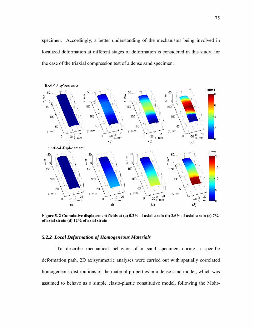
75
specimen. Accordingly, a better understanding of the mechanisms being involved in
localized deformation at different stages of deformation is considered in this study, for
the case of the triaxial compression test of a dense sand specimen.
Figure 5. 2 Cumulative displacement fields at (a) 0.2% of axial strain (b) 3.6% of axial strain (c) 7% of axial strain (d) 12% of axial strain
5.2.2 Local Deformation of Homogeneous Materials
To describe mechanical behavior of a sand specimen during a specific
deformation path, 2D axisymmetric analyses were carried out with spatially correlated
homogeneous distributions of the material properties in a dense sand model, which was
assumed to behave as a simple elasto-plastic constitutive model, following the Mohr-
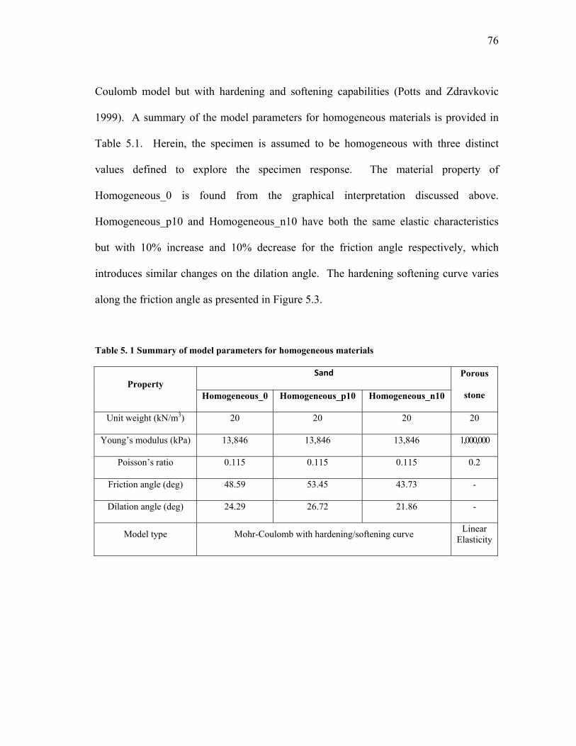
76
Coulomb model but with hardening and softening capabilities (Potts and Zdravkovic
1999). A summary of the model parameters for homogeneous materials is provided in
Table 5.1. Herein, the specimen is assumed to be homogeneous with three distinct
values defined to explore the specimen response. The material property of
Homogeneous_0 is found from the graphical interpretation discussed above.
Homogeneous_p10 and Homogeneous_n10 have both the same elastic characteristics
but with 10% increase and 10% decrease for the friction angle respectively, which
introduces similar changes on the dilation angle. The hardening softening curve varies
along the friction angle as presented in Figure 5.3.
Table 5. 1 Summary of model parameters for homogeneous materials
Property Sand Porous
stone Homogeneous_0 Homogeneous_p10 Homogeneous_n10
Unit weight (kN/m3) 20 20 20 20
Young’s modulus (kPa) 13,846 13,846 13,846 1,000,000
Poisson’s ratio 0.115 0.115 0.115 0.2
Friction angle (deg) 48.59 53.45 43.73 -
Dilation angle (deg) 24.29 26.72 21.86 -
Model type Mohr-Coulomb with hardening/softening curve Linear
Elasticity

77
Figure 5. 3 Hardening and softening curve for homogeneous materials
A comparison of the global specimen’s behavior vs. predictions of the finite
element model is presented in Figure 5.4. Since material property of Homogeneous_0 is
based on the global behavior of an actual triaxial test, the stress-strain curve is the closet
to the actual test results. Model Homogeneous_p10 has the highest peak stress and
Homogeneous_n10 shows the behavior of an elasto-perfectly plastic material.
Homogeneous_p10 has excessive volumetric strain and Homogeneous_n10 shows the
closest strain curve to the strain curve of the actual test at a peak stress, followed closely
by Homogeneous_0. After the peak stress, the gap of volumetric strain between the test
result and finite element models decreases.

78
Figure 5. 4 Global stress-strain behavior of homogeneous materials
Averaged radial and axial displacements at 3.6% and 7% of axial strain are used
as benchmarks to compare model predictions vs. actual displacement fields as showed in
Figure 5.5. This includes cumulative density functions of the corresponding
displacement errors. The difference between the actual test and the model predictions
are more evident at 3.6% of axial strain when comparing radial displacements. However,
for vertical displacement deviations at the peak are not as significant as after the peak.
Results showed better agreement on the vertical than in the radial displacements, with
higher and unbiased deviations at the peak for the radial displacements over the
tangential displacement, and similar unbiased deviations for both the radial and the
tangential after the peak.

79
Figure 5. 5 Displacements and cumulative density function at 3.6% and 7% of axial strain (a) radial displacement (b) cumulative density function of radial displacement errors (c) axial displacement (d) cumulative density function of axial displacement errors
5.3 Mesh Sensitivity Analysis in Plastic Straining
5.3.1 Problem Definition
The research by Read and Hegemier (1984) used experimental observations to
provide a comprehensive review about strain softening with respect to the effects of
specimen size and shape. They concluded that the strain softening is not a real property
of materials but rather, the results of inhomogeneous deformation that can be constructed

80
with a sufficiently small size of material elements. Therefore, a finite element method is
proposed for numerically analyzing the behavior of materials which show strain
softening. However, for numerical approaches on elasto-plastic materials, the numerical
solutions suffer from instability and finite element mesh size sensitivity in stress-strain
or load-displacement responses when the material enters the strain softening range. This
has been acknowledged by numerous researchers and a number of approaches have been
proposed to overcome these difficulties.
Pietruszczak and Mroz (1981) formulated the stiffness matrix accounting for the
thickness of a shear band of the Coulomb-softening material in plane strain condition.
They also showed the load-displacement curves are not sensitive to the mesh size used in
the proposed model, compared to the results of a conventional finite element model that
show high sensitivity in both the limit load and the slope of strain softening.
Pietruszczak and Stolle (1985) discussed the influence of discretization of the finite
element mesh and presented the results of the footing problem solved by the constitutive
relationship suggested by Pietruszczak and Mroz (1981). Steinmann and William (1991)
performed a convergence study of compressive failure for an elasto-plastic material
under a plane strain condition. Although the peak point predictions correspond, the post
peak response indicates mesh sensitivity and the localization performance of different
elements.
Another finite element implementation of strain softening is an application of a
damage variable in constitutive relations. Frantziskonis and Desai (1987a) proposed a
model that separates the behavior of a material into the continuum part and the damaged

81
part. The damaged part is softened because of the accumulation of damage. The finite
element solutions obtained by using the proposed model were not sensitive to the
changes in mesh size for material response predictions (Frantziskonis and Desai 1987b).
Recently, finite element methods based on the discontinuities in displacements or
strains are introduced for the localization analysis, which is caused by material
instability (Borja 2000; Wells et al. 2002). The gradient regularization is also considered
for finite element simulations of shear band formation during strain softening (de Borst
et al. 1993; Anand et al. 2012).
In this study, numerical simulations of a drained triaxial compression test using a
two-dimensional finite element model were carried out to calibrate an elasto-plastic soil
constitutive model. Results from the numerical simulations are used to discuss the
sensitivity of mesh discretization in terms of the material behavior. For the numerical
analysis of the problem, robustness in the numerical solution for an elasto-plastic
simulation of the soil specimen is difficult to expect, because numerical instability in a
stress-strain response in the case of dense sands can be attributed to plastic straining
effects. To characterize the extent of the sensitivity of these effects, a parametric study
is introduced.
Previous studies on the similar problem related to the numerical modeling for
granular materials are more focused on the model prediction in global behavior, by
comparing the global stress-strain and volumetric strain predictions with respect to the
test data (Wan and Guo 1998; Cameron and Carter 2009). Other studies related to the
numerical simulation of a drained triaxial compression test are focused on the discrete

82
element modeling of the problem dealing with the characteristics of sand grains and its
physical properties as a model parameter (Chang and Hicher 2005; Belheine et al. 2009).
However, this study is focused on the investigation of the localized deformation
effects measured on the boundary of dense sand specimens by comparing the model
predictions with experimental data. This comparison demonstrates the ability of the
model to reproduce accurately the overall mechanical behavior of the specimens and to
take into account the influence of local effects by an improved definition of mechanical
parameters obtained by a three-dimensional digital image correlation analysis (3D-DIC),
which is used to generate 3D local kinematic information retrieved from the deforming
specimen.
5.3.2 Effects of Mesh Discretization
The actual process of the compression triaxial test, in terms of the initial and
boundary conditions related to testing procedures and calibration of parameters was
simulated via a finite element analysis. Under certain conditions based on the actual
shearing process, the finite element analyses for typical dense sands are affected by the
determination of the mesh discretization, such as element type and mesh size. The
material behavior, in particular the plastic straining incorporating strain softening, is
attributed to the sensitivity of this discretization. Therefore, the finite element model
prediction was analyzed to quantify the effects of element type and mesh size. Figure
5.6 illustrates all the mesh types and sizes of the 2D models used in the parametric study.
Mesh sizes of 3 mm, 5 mm, 10 mm, 20 mm, and 40 mm respectively, were used to vary

83
the number of elements, using triangular (denoted as ‘tr’) and rectangular (denoted as
‘sq’) elements. A summary describing the test cases is presented in Table 5.2.
Figure 5. 6 Mesh discretization of 2D finite element models (a) 3mm_tr, 3mm_sq (b) 5mm_tr, 5mm_sq (c) 10mm_tr, 10mm_sq (d) 20mm_tr, 20mm_sq (e) 40mm_tr, 40mm_sq
Table 5. 2 Test cases for mesh sensitivity analysis
Name No. of
nodes
No. of
elements
Mesh size
(mm) Element type
3mm_tr_3 754 1,368 3 a 3-node linear triangle
3mm_tr_6 2,875 1,368 3 a 6-node quadratic triangle
3mm_sq_4 754 684 3 a 4-node bilinear rectangle
3mm_sq_8 2,191 684 3 an 8-node biquadratic rectangle
5mm_tr_3 280 476 5 a 3-node linear triangle
5mm_sq_8 797 238 5 an 8-node biquadratic rectangle

84
Table 5.2 continued
Name No. of
nodes
No. of
elements
Mesh size
(mm) Element type
10mm_tr_3 95 144 10 a 3-node linear triangle
10mm_sq_8 261 72 10 an 8-node biquadratic rectangle
20mm_tr_3 33 40 20 a 3-node linear triangle
20mm_sq_8 85 20 20 an 8-node biquadratic rectangle
40mm_tr_3 14 12 40 a 3-node linear triangle
40mm_tr_6 39 12 40 a 6-node quadratic triangle
40mm_sq_4 14 6 40 a 4-node bilinear rectangle
5.3.3 Effects of Element Type
The effects of element type are first examined by analyzing the global stress-
strain behavior of the specimen. Four element types are compared when using 3mm and
40mm mesh sizes. As shown in Figure 5.7 (a), an 8-node biquadratic rectangle (sq_8)
element generates a better prediction than a 3-node linear triangle (tr_3) element. This
result shows the effects of the number of nodes and the number of integration points.
With the higher order elements, or the more number of nodes, the prediction of the
maximum stress is more accurate and the variation of stress at the critical state is also
smaller. Another finding is that the results of fine mesh size (Figure 5.7 (a) and (b)) are
nearly insensitive to the element type, as seen by the similar model predictions. In
contrast, a coarse mesh (Figure 5.7 (c) and (d)) affects significantly the element type, as
seen by the disparity in the stress strain curves.

85
Figure 5. 7 Effects of element type on global stress-strain behavior
(a) (b)
Mesh size, 3mm
( )( )( )( )
( )( )( )( )
Peak 3.6% Critical 12% Peak 3.6% Critical 12%
(c) (d)
Mesh size, 40mm
( )( )( )( )
(b)
( )( )( )( )
Peak 3.6% Critical 12% Peak 3.6% Critical 12%

86
5.3.4 Effects of Mesh Size
Figure 5.8 presents a comparison of the global stress-strain behavior due to
different mesh sizes. The mesh size has an effect on the maximum stress and
corresponding axial strain. For the coarse mesh, the magnitude of the maximum stress is
higher and the slope of strain softening curve is decreasing, which constitutes an
inaccurate prediction. For instance, the test 40mm_tr_3 in Figure 5.8 (a) does not
exhibit a strain softening behavior, even though the softening law was imposed, and the
stress difference between the prediction of the test 40mm_tr_3 and the experimental
curve at the critical state is 120kPa. The axial strain at the maximum stress is, therefore,
increasing as the mesh size becomes larger. Even though the influence of mesh size is
significant on predicting stresses, the variation of the volumetric strain in the models is
relatively small. The trends shown in Figure 5.7 and 5.8, presenting the peak stress and
strain softening after peak are affected by both the number and type of elements, are in
agreement with those by Petruszczak and Mroz (1981) and Petruszczak and Stolle
(1985).

87
Figure 5. 8 Effects of mesh size on global stress-strain behavior
An innovative comparison now, is the analysis of the averaged radial and vertical
displacements, representing the local kinematic effects. For instance, these
displacements at the peak (3.6% of axial strain) and critical state (12% of axial strain)
are used as benchmarks to compare model predictions as showed in Figure 5.9 and 5.10

88
respectively. The displacement errors (Figure 5.9 (b), (d) and 5.10 (b), (d) ) indicate the
difference between predictions and actual displacements.
Figure 5. 9 Displacements and displacement errors at peak: (a) radial displacement (b) radial displacement errors (c) vertical displacement (d) vertical displacement errors

89
The difference between the actual test and the model predictions is relatively
higher at the peak values when comparing radial displacements. The radial displacement
predictions are distributed symmetrically around the middle of the specimen height.
However, for vertical displacement, deviations at the peak are not as significant. Notice
that the order of magnitude on the radial displacements is around 0.8 mm for the radial
displacements, and 0.3 mm for the vertical displacements.
After the peak, the deformation within the specimen tends to localize along
concentrated shear bands, and the relative differences between the experimental
observations and the model prediction are relatively small for both the radial and vertical
displacements. Due to the movement of the bottom one third of a specimen, the radial
displacement error dramatically decreased at a height of 40mm. Notice the effect on the
directionality of the triangular coarse mesh, such as the test 40mm_tr_3 (Figure 5.11
(3)), which imposes an effect on the location of maximum displacements, thus it causes
an inaccurate prediction of displacements.

90
Figure 5. 10 Displacements and displacement errors at critical state: (a) radial displacement (b) radial displacement errors (c) vertical displacement (d) vertical displacement errors

91
Figure 5. 11 Deformed meshes with horizontal displacement contour
5.3.5 Stress and Strain Cross Sections
The deviatoric stress and plastic strain distribution in different stress states are
illustrated in Figure 5.12, which describes the variation inside the specimen. The Mises
equivalent stress is defined as (2/3) S:S , where S=the stress deviator and the symbol (:)
denotes a scalar product operation. The plastic strain magnitude, PEMAG is defined as
pl pl(2/3) ε :ε , where plε =plastic strain.
While the deviatoric stresses at the peak and critical state in a global stress-strain
curve are respectively 230kPa and 210kPa as shown in Figure 5.8 (c), the Mises stress
ranges between 150kPa to 570kPa in Figure 5.12 (a). A stress concentration is observed
at the center of the model specimen 100mm from the bottom, and the concentrated stress

92
diagonally dissipates with regard to strain softening. Figure 5.12 (b) indicates a
significant increase in the plastic strain which is a result of strain softening as well. The
deformation tends to localize along concentrated shear bands propagating within the
specimen. On the other hand, these trends can be explained in terms of the material
strength. The displacement load applied after the peak resulted in the increased
deformation of the specimen due to the decreased strength of material.
Figure 5. 12 Deviatoric stress and plastic strain distribution of test 3mm_sq_8 at peak and critical state (a) deviatoric stress (b) plastic strain

93
5.4 Comparative Analysis among Dense, Loose and Layered Sand Specimens
5.4.1 Experimental Comparison
This study presents an elasto-plastic comparative analysis of different sand
specimen configurations, including loose, dense and layered (half-loose half-dense)
specimens. Experimental conditions were simulated by a finite element model with an
elasto-plastic constitutive model, to investigate the elasticity and hardening plasticity
responses of sand specimens during a triaxial test. Calibration of the numerical models
for each specimen condition was based on the use of boundary information of the
kinematics generated by 3D digital image correlation analysis. The photo images and
cumulative displacement fields at the elastic and critical states are presented in Figure
5.13 and 5.14. In the elastic state, samples are compressed so radial displacement fields
show negative values. Axial displacement fields are linearly distributed except in the
case of the layered specimen in which the lower segment moves at the rate of loading
and upper segment is compressed. The direction of shearing and the onset of shear
bands can be estimated from tangential displacement fields.
A shear band of a dense sand specimen is clearly observed at the critical state and
as the bottom segment of the specimen is separated from the bulging surface of the
specimen by shearing, and then it moves independently as a single block. A loose
specimen deformed symmetrically without shearing but bulging in radial direction is
observed and this implies that the occurrence of bulging may cause an increase of
volume. At the lower segment of the layered specimen, radial and tangential

94
displacements are not significant. The upper segment of the specimen shows a relatively
significant deformation, which means that the deformation is concentrated on the weak
part, i.e. the upper segment.
Figure 5. 13 3D digital image correlation analysis at 0.2% of axial strain (elastic state)

95
Figure 5. 14 3D digital image correlation analysis at 12% of axial strain (critical state)
Global stress-strain and volumetric strain curves are presented in Figure 5.15.
The global behavior of a layered specimen that consists of two layers with different
densities but the same heights shows a typical behavior of a loose specimen and even the
maximum stress is also close to the maximum stress of the loose specimen. This means
that the kinematic characteristics of the multi-layered soil structure are controlled by a
weak layer, and averaged material parameters of all layers will overestimate the actual
global behavior though depth of layers are considered.

96
Volumetric strains of the loose and layered specimens show dilation like a dense
sand specimen in Figure 5.15 (b). Relative densities of loose and layered specimens are
46.39% and 68.90% respectively. Note that the relative density of the layered specimen
is an average value that was computed from the total volume of the specimen. The
condition of granular materials can be determined by relative density. The material with
15% to 50% of relative density is defined as a loose material, and with 50% to 70% of
relative density it is defined as a medium material (Das 2001). Also, some experimental
data of sands with relative density between 42% and 47% shows dilation in global
volumetric strain behavior (Finno and Rechenmacher 2003). If these two samples are
assumed as medium material, this dilation phenomenon in volume can be explained.
Figure 5. 15 Comparison between experimental results (a) deviatoric stress vs. axial strain curve (b) volumetric behavior vs. axial strain

97
5.4.2 2D Axisymmetric Finite Element Modeling
For a simulation of triaxial tests on sand specimens, a 2D axisymmetric finite
element model is adopted. Dense and loose specimens are modeled as homogeneous
materials. A layered specimen is analyzed in both homogeneous and heterogeneous
materials considering the specimen configurations. For a layered specimen, three cases
are considered: a homogeneous material using the global kinematics captured in Figure
5.15, a heterogeneous material with two layers of loose and dense sands as built in
experimental sample preparation, and another heterogeneous condition considering
transition zone between loose and dense sands (Figure 5.16).
Figure 5. 16 Sand specimen configurations (a) dense specimen (b) loose specimen (c) layered specimen modeled with a homogeneous material (layered_hom) (d) layered specimen consists of two layers (layered_het) (e) layered specimen considering a transition zone (layered_het_transition)

98
A summary of material properties for dense, loose and layered samples is
presented in Table 5.4. For a lower dense segment, the properties of a dense specimen
are adopted since both are very dense materials. However, the upper loose segment
requires a modification of the properties of a loose specimen because the loose sample
has the characteristics of a medium material but the upper segment may behave more
like a loose material. Duncan (2004) suggested an equation for an estimate of the
friction angle from an experimental database of relative density, grain size, particle
gradation and pressure as a form of Nr r 10
a
σ=Α+Β(D )-[C+D(D )]log
P
, where Dr is a
relative density, Nσ is a confining pressure, and aP is the standard atmospheric pressure
of 101.325kPa. The coefficients A, B, C, and D that are dependent on the material type
are presented in Table 5.3.
Table 5. 3 Coefficients for an estimation of the friction angle (Duncan, J.M. 2004)
Material type A B C D Standard deviation
Gravel with Cu>4 44 10 7 2 3.1°
Sand with Cu>6 39 10 3 2 3.2°
Sand with Cu<6 34 10 3 2 3.2°
Using the equation, the friction angle for the upper loose segment is determined
to 38.51° with a standard deviation of 3.2° at the critical state. Since friction angles used
for a finite element analysis are computed at the elastic limit, it may be smaller than the
friction angles at the critical state. Thus the ratio of the friction angle of the upper

99
segment to the friction angle of the loose sample at the critical state is used to modify the
hardening/softening curve of the loose sample. The adopted hardening and softening
curve is presented in Figure 5.17. The parameters of the transition zone are computed by
averaging two global stress-strain curves of loose and dense specimens.
Table 5. 4 Summary of material properties for dense, loose and layered specimens
Name Unit
weight (kN/m3)
Young’s modulus
(kPa)
Poisson’s ratio
Friction angle (deg)
Dilation angle (deg)
Relative density
(%)
Note
Dense 20 21,559 0.44 43.09 22.78 91.83 homogeneous
Loose 20 15,818 0.25 32.86 14.48 46.39 homogeneous
Layered
_hom Medium 20 18,164 0.2 32.12 11.97 68.90 homogeneous
Layered
_het
Upper
loose 20 15,818 0.25 32.86 14.48 30.54
heterogeneous,
two layers Lower
dense 20 21,559 0.44 43.09 22.78 98.87
Layered
_het
_transition
Upper
loose 20 15,818 0.25 32.86 14.48 30.54
heterogeneous,
three layers
including
transition zone
Transition
zone 20 20,361 0.37 36.86 18.19 -
Lower
dense 20 21,559 0.44 43.09 22.78 98.87
Porous stone 20 1,000,000 0.2 - - - linear elasticity

100
Figure 5. 17 Hardening and softening curves for (a) dense specimen (b) loose specimen, upper loose segment of layered_het model, and layered_hom model
5.4.3 Comparative Results
Figure 5.18 and 5.19 illustrated model predictions with experimental results.
Results show that the numerical model predictions are in good agreement with the
laboratory tests in terms of stress. With respect to volumetric strain, compression in
elastic state is underestimated by adopting a tangential elastic modulus for a better
prediction of stress in the elastic state. For a layered specimen, ‘layered_hom’ test
shows the best fit to global behavior of a laboratory test and other two heterogeneous
models shows about 10 to 20kPa of deviation in a stress-strain curve. It may be occurred
because of the deviation in the estimation of the friction angle or neglect of a difference
of material properties between a dense specimen and the lower dense segment.

101
Figure 5. 18 Model predictions in global behavior for dense and loose specimens
(a) stress-strain curve (b) axial strain vs. volumetric strain
Figure 5. 19 Model predictions in global behavior for a layered specimen
Local deformation of a layered specimen at 12% of axial strain, i.e. critical state
is analyzed in Figure 5.20 and 5.21. Contrary to the global behavior, homogeneous
model (layered_hom) shows symmetric deformation in radial direction and it proves the
necessity of a heterogeneous model. The first heterogeneous model with two layers,
‘layered_het’ shows a similar trend of displacement distribution in both radial and

102
vertical directions. However, at a height between 40mm and 80mm, the model
deformation is too stiff to fit the laboratory results. Thus, heterogeneous model
(layered_het_transition) introduced a transition zone of 40mm between the upper and
lower segments to allow for changes in the stiffness of sands. The
layered_het_transition model has better agreement with minor deviations of 1mm in both
the radial and vertical displacements rather than the other two layered model predictions.
Figure 5. 20 Radial displacement distributions and its errors (a) radial displacement distribution (b) radial displacement errors

103
Figure 5. 21 Vertical displacement distributions and its errors (a) vertical displacement distribution (b) vertical displacement errors
Total displacement vectors and a deformed mesh of layered specimen prediction
models are illustrated in Figure 5.22. The homogeneous model, layered_hom, is
deformed in a shape of a barrel like a loose sand. In the heterogeneous models,
layered_het and layered_het_transition, deformations mainly occurred in the loose
specimen section.

104
Figure 5. 22 Total displacement vectors (a) layered_hom (b) layered_het (c) layered_het_transition

105
6. CONCLUSIONS
3D digital image correlation provides local displacement information that enables
the determination of model parameters for the modeling of local kinematic effects. After
the digital image correlation, post-processing analyses was performed to better align the
initial undeformed state with the coordinate system, and to accumulate displacements
from the step-wise analyses required to populate the local kinematic effects. The
deformation of a representative volume of the material captured by 3D-DIC is used for
the estimation of the kinematic and volumetric conditions of the specimen at different
stages of deformation, combined with the readings of the global axial compression of the
specimen, which allow for the characterization of the Mohr-Coulomb plasticity model
with hardening and softening laws.
A 2D axisymmetric finite element model was proposed as a first approach to
replicate the local effects. This included an elasto-plastic constitutive model with
hardening and softening capabilities. Results of the finite element model showed better
agreement on the vertical than in the radial displacements, with higher and unbiased
deviations at the peak for the radial displacements over the tangential displacement, and
similar unbiased deviations for both the radial and the tangential after the peak.
In order to provide sensitivity of mesh discretization in strain softening, a
parametric study of a 2D finite element model was carried out to examine the effects of
element type and mesh size. Higher order element types and fine mesh sizes produce
more accurate stress and displacement distribution predictions. Another relevant

106
observation from this investigation was that after the peak strength was reached, the
deformation within the specimen tended to localize and became more sensitive to mesh
discretization. Still finite element models, with a homogeneous material, have a
limitation in modeling non-symmetric displacement distributions by shearing after the
peak stress, but give useful information on the variation of plastic strain and stress inside
of the specimen.
A comparative analysis of different specimen configurations was performed
using a 2D finite element model. The model parameters for an elasto-plastic.model with
hardening and softening law were calibrated from the global kinematics of dense and
loose specimens. A layered specimen consists of two layers with different relative
densities so the material parameters of the two layers were obtained from dense and
loose specimens with modifications in a hardening and softening curve. The
heterogeneous model with transition zone between loose and dense segments presented
better predictions on the local deformation of the layered specimen.

107
REFERENCES
ABAQUS Inc. (2008). ABAQUS user’s manual, version 6.8, Hibbitt, Karlsson, and
Sorensen., Pawtucket, RI.
Abbo, A.J. (1997). Finite element algorithms for elastoplasticity and consolidation,
Ph.D. dissertation, The University of Newcastle, New South Wales, Australia.
Almeida, O.D., Lagattu, F., and Brillaud, J. (2008). “Analysis by a 3D DIC technique of
volumetric deformation gradients: Application to polypropylene/EPR/talc
composites.” Composites Part A: Applied Science and Manufacturing, 39(8),
1210-1217.
Anand, L., Aslan, O., and Chester, S.A. (2012), “A large-deformation gradient theory for
elastic-plastic materials: Strain softening and regularization of shear bands.”
International Journal of Plasticity, 30-31, 116-143.
Atkinson, J.H. and Bransby, P.L. (1978). The mechanics of soils: an introduction to
critical state soil mechanics. McGraw-Hill, London, UK.
Bayoumi, A. (2006). New laboratory test procedure for the enhanced calibration of
constitutive models, Ph.D. dissertation, Georgia Institute of Technology, Atlanta,
GA.
Belheine, N., Plassiard, J.-P., Donze, F.-V., Darve, F., and Seridi, A. (2009). “Numerical
simulation of drained triaxial test using 3D discrete element modeling.”
Computers and Geotechnics, 36(1-2), 320-331.

108
Brinkgreve, R.B.J. (2005). “Selection of Soil Models and Parameters for Geotechnical
Engineering Application.” Soil Constitutive Models: Evaluation, Selection, and
Calibration, Geotechnical Special Publications, 128, 69-98.
Boldyrev, G.G., Idrisov, I.Kh., and Valeev, D.N. (2006). “Determination of parameters
for soil models.” Soil Mechanics and Foundation Engineering, 43(3), 101-108.
Borja, R.I. (2000). “A finite element model for strain localization analysis of strong
discontinuous fields based on standard Galerkin approximation.” Computer
Methods in Applied Mechanics and Engineering, 190(11-12). 1529-1549.
Cameron, D.A. and Carter, J.P. (2009). “A constitutive model for sand based on non-
linear elasticity and the state parameter.” Computers and Geotechnics, 36(7),
1219–1228.
Chang, C.S. and Hicher, P.-Y, (2005). “An elasto-plastic model for granular materials
with microstructural consideration.” International Journal of Solids and
Structures, 42(14), 4258–4277.
Charalampidou, E.M., Hall, S.A., Stanchits, S., Viggiani, G., and Lewis, H. (2010).
“Experimental characterization of shear and compaction band mechanisms in
porous sandstone by a combination of AE and 3D DIC.” 14th International
Conference on Experimental Mechanics, Poitiers, France, EPJ Web of
Conferences, 6.
Chupin, O., Rechenmacher, A.L., and Abedi, S. (2011). “Finite strain analysis of
nonuniform dieformation inside shear bands in sands.” International Journal for
Numerical and Analytical Methods in Geomechanics.

109
Correlated Solutions, Inc. (2010). VIC-3D, Columbia, SC.
Das, B. M. (2001). Principles of geotechnical engineering, 5th edition, Thomson
Learning, Pacific Grove, CA.
de Borst, R., Sluys, L.J., Muhlhaus, H.-B., and Pamin, J. (1993). “Fundamental issues in
finite element analyses of localization of deformation.” Engineering
Computations, 10(2), 99-121.
Dean, G. and Crocker, L. (2001). “The use of finite element methods for design with
adhesives.” NPL Good Practice Guide, 48, Teddington, UK.
Desai, C.S. and Siriwardane, H.J. (1984). Constitutive laws for engineering materials:
with emphasis on geologic materials, Prentice-Hall, Englewood Cliffs, NJ.
Desrues, J. (1996) “Localisation patterns in ductile and brittle geomaterials.” Material
Instabilities in Solids, 137-158.
Desrues, J. and Viggiani, G. (2004). “Strain localization in sand: an overview of the
experimental results obtained in Grenoble using stereophotogrammetry.”
International Journal for Numerical and Analytical Methods in Geomechanics,
28(4), 279-321
Duncan, J.M. (1994). “The role of advanced constitutive relations in practical
applications.” Proceedings, 13th International Conference Soil Mechanics and
Foundation Engineering, New Delhi, India, 5, 31-48.
Duncan, J.M. (2004). “Friction angles for sand, gravel and rockfill.” Notes of a lecture
presented at the Kenneth L. Lee Memorial Seminar, Long Beach, CA.

110
Finno, R.J. and Rechenmacher, A.L. (2003). “Effects of consolidation history on critical
state of sand.” Journal of Geotechnical and Geoenvironmental Engineering,
129(4), 350-360.
Foley, J.D., van Dam, A., Feiner, S.K., and Hughes, J.F. (1996). Computer graphics:
principles and practice in C. 2nd edition, Addison-Wesley Professional, New
York, NY.
Frantziskonis, G. and Desai, C.S. (1987a). “Constitutive model with strain softening.”
International Journal of Solids and Structures, 23(6), 733-750.
Frantziskonis, G. and Desai, C.S. (1987b). “Analysis of a strain softening constitutive
model.” International Journal of Solids and Structures, 23(6), 751-767.
Fredlund, D.G., Xing, A., Frelund, M.D., and Barbour, S.L. (1996). “The relationship of
the unsaturated soil shear strength function to the soil-water characteristic curve.”
Canadian Geotechnical Journal, 33(3), 440-448.
Gay, O., Boutonnier, L., Foray, P., and Flavigny, E. (2003). “Laboratory characterization
of Hostun RF sand at very low confining stresses.” Deformation Characteristics
of Geomaterials, Di Benedetto et al. eds., 423-430.
Helwany, S. (2007). Applied soil mechanics: with ABAQUS applications, John Wiley &
Sons, Hoboken, NJ.
Hicher, P.Y. and Shao, J.F. (2008). Constitutive modeling of soils and rocks, John Wiley
& Sons, Hoboken, NJ.
Holtz, R.D. and Kovacs, W.D. (1981). An introduction to geotechnical engineering,
Prentice-Hall, Englewood Cliffs, NJ.

111
Iskander, M. (2010). Modelling with transparent soils: visualizing soil structure
interaction and multi phase flow, non-intrusively, Springer Series in
Geomechanics and Geoengineering, Springer-Verlag Berlin Heidelberg, New
York, NY.
Lade, P.V. (2005). “Overview of constitutive models for soils.” Soil constitutive models:
Evaluation, selection and calibration, Yamamuro, J.A. and Kalaikin, V.N. eds.,
ASCE Geotechnical Special Publication, No.128, 1-34.
Lava, P., Coppieters, S., Wang, Y., Van Houtte, P., and Debruyne, D. (2011). “Error
estimation in measuring strain fields with DIC on planar sheet metal specimens
with a non-perpendicular camera alignment.” Optics and Laser in Engineering,
49(1), 57-65.
Macari, E.J., Parker, J.K., and Costes, N.C. (1997). “Measurement of volume changes in
triaxial tests using digital imaging techniques.” Geotechnical Testing Journal,
GTJODJ, 20(1), 103-109.
McNeill, S.R., Sutton, M.A., Miao, Z., and Ma, J. (1997). “Measurement of surface
profile using digital image correlation.” Experimental Mechanics, 37(1), 13-20.
Medina-Cetina, Z. (2006). Probabilistic calibration of soil constitutive models, Ph.D.
dissertation, Johns Hopkins University, Baltimore, MD.
Medina-Cetina, Z. and Rechenmacher, A. (2010). “Influence of boundary conditions,
specimen geometry and material heterogeneity on model calibration from triaxial
tests.” International Journal for Numerical and Analytical Methods in
Geomechanics, 34(6), 627-643.

112
Nuth, M. and Laloui, L. (2008), “Effective stress concept in unsaturated soils:
Clarification and validation of a unified framework.” International Journal for
Numerical and Analytical Methods in Geomechanics, 32(7), 771-801.
Peterson, R.F.W. (1988). “Interpretation of triaxial compression test results on partially
saturated soils.” Advanced Triaxial Testing of Soil and Rock, American Society
for Testing and Materials, ASTM STP 977, 512-538.
Pietruszczak, ST. and Mroz, Z. (1981). “Finite element analysis of deformation of strain-
softening materials.” International Journal for Numerical Methods in
Engineering, 17(3), 327-334.
Pietruszczak, ST. and Stolle, D.F.E. (1985). “Deformation of strain softening materials.
Part I: Objectivity of finite element solutions based on conventional strain
softening formulations.” Computer and Geotechnics, 1(2), 99-115.
Potts, D.M. and Zdravkovic, L. (1999). Finite element analysis in geotechnical
engineering: Volume 1-Theory, Thomas Telford Publishing, London, UK.
Potts, D.M. (2003). “Numerical analysis: a virtual dream or practical reality?”
Géotechnique, 53(6), 535-573.
Powrie, W. (1997). Soil mechanics: concepts and applications, E&FN Spon, Oxford,
UK.
Read, H.E. and Hegemier, G.A. (1984). “Strain softening of rock, soil and concrete – A
review article.” Mechanics of Materials, 3(4), 271-294.
Rechenmacher, A.L. (2006). “Grain-scale processes governing shear band initiation and
evolution in sands.” Journal of the Mechanics and Physics of Solids, 54(1), 22-45.

113
Schofield, A.N. and Wroth, P. (1968). Critical state soil mechanics, McGraw-Hill, New
York, NY.
Sloan, S.W., Abbo, A.J., and Sheng, D., (2001). “Refined explicit integrateion of
elastoplastic models with automatic error control.” Engineering Computations,
18(1-2), 121-154.
Sloan, S.W. and Booker, J.R., (1986). “Removal of singularities in Tresca and Mohr-
Coulomb yield functions.” Communications in Applied Numerical Methods, 2(2),
173-179.
Steinmann, P. and William, K. (1991). “Performance of enhanced finite element
formulations in localized failure computations.” Computer Methods in Applied
Mechanics and Engineering, 90(1-3). 845-867.
Sutton, M.A., McNeill, S.R., Helm, J.D., and Chao, Y.J. (2000). “Advances in two-
dimensional and three-dimensional computer vision.” Photomechanics (Topics in
Applied Physics), Rastogi, P.K. ed., 77, 323-372.
Sutton, M.A., Yan, J.H., Tiwari, V., Schreier, H.W., and Orteu, J.J. (2008). “The effect
of out-of-plane motion on 2D and 3D digital image correlation measurements.”
Optics and Lasers in Engineering, 46(10), 746-757.
Tai, Y.H., Zanganeh, M., Asquith, D., and Yates, J.R. (2010). “Characterisation of full-
field deformation behaviour using digital imaging techniques.” Applied
Mechanics and Materials, AMM, 24-25, 141-146.
The MathWorks, Inc. (2009). MATLAB version R2009b, Natick, MA.

114
Vesic, A.S., and Clough, G.W. (1968). “Behaviour of granular material under high
stresses.” Journal of Soil Mechanics Foundation Devision, 94, 661-688.
Wan, R.G., and Guo, P.J. (1998). “A simple constitutive model for granular soils:
Modified stress-dilatancy approach.” Computers and Geotechnics, 22(2), 109-
133.
Wells, G.N., Sluys, L.J., and de Borst, R. (2002). “Simulating the propagation of
displacement discontinuities in a regularized strain-softening medium.”
International Journal for Numerical Methods in Engineering, 53(5), 1235-1256.
Zienkiewicz, O.C. and Taylor, R.L. (2000). The finite element method: Volume 1. Basic
formulation and linear problems, Volume 2. Solid mechanics, 5th edition,
Butterworth-Heinemann, Woburn, MA.

115
VITA Name: Ahran Song
Address: Zachry Department of Civil Engineering Texas A&M University College Station, TX 77843-3136 Email Address: [email protected] Education: B.S., Civil and Environmental Engineering, Sungkyunkwan University, South Korea, 2005 M.S., Geotechnical Engineering, Sungkyunkwan University, South Korea, 2007 Ph.D., Geotechnical Engineering, Texas A&M University, 2012