Delayed Detached–Eddy Simulation of Shock Buffet

on Half Wing–Body Configuration

F. Sartor∗ and S. Timme†

University of Liverpool, Liverpool, England L69 3GH, United Kingdom

This paper presents a numerical study of the transonic flow over a half wing-body con-figuration representative of a large civil aircraft. The Mach number is close to cruiseconditions, while the high angle of attack causes massive separation on the suction sideof the wing. Results indicate the presence of shock-wave oscillations inducing unsteadyloads which can cause serious damage to the aircraft. Transonic shock buffet is found.Based on preliminary simulations using a baseline grid, the region relevant to the phe-nomenon is identified and mesh adaptation is applied to significantly refine the grid locally.Then, time-accurate Reynolds-averaged Navier-Stokes and delayed detached-eddy simula-tions are performed on the adapted grid. Both types of simulation reproduce the unsteadyflow physics and much information can be extracted from the results when investigatingfrequency content, the location of unsteadiness and its amplitude. Differences and similar-ities in the computational results are discussed in detail and also analysed with respect torecent experimental data.

I. Introduction

At cruise condition, the flow around the wing of a typical large civil aircraft is characterised by thepresence of strong shock waves interacting with the boundary layer to cause massive separation. The conse-quence is the occurrence of large-scale unsteadiness including significant shock movements, known as shockbuffet, which arise for combinations of Mach number and angle of attack.1 This phenomenon presents anindustrial interest and has thus been the subject of numerous studies in the past.

Shock buffet is a phenomenon that can be observed both in two- and three-dimensional configurations,from simple aerofoils to swept wings. In the particular two-dimensional case, the unsteadiness is characterisedby harmonic shock motions. There is a large amount of literature discussing experimental investigations,2,3, 4

numerical studies based on unsteady Reynolds-averaged Navier-Stokes (URANS) simulations,5,6, 7 and sta-bility analysis.8,9, 10 More recently, high-fidelity approaches based on hybrid methods such as zonal detached-eddy simulation (ZDES),11 delayed detached-eddy simulation (DDES)12 or improved delayed detached-eddysimulation13 have successfully been applied to two-dimensional profiles.

When considering more challenging configurations, such as a wing representative of a large civil aircraft,the literature is more limited. Experimental investigations have shown the complexity of the shock motions14

and were able to demonstrate the potential benefit of control devices.15,16 Several numerical studies havetried to characterise the three-dimensional buffet on a complete wing. Some authors have simulated theshock unsteadiness using ZDES and have argued that a URANS approach is not suited to reproduce thecomplex phenomenon of three-dimensional buffet.17 A similar conclusion was drawn from the first AeroelasticPrediction Workshop,18 where RANS simulations were shown to be insufficient for the correct physicalmodelling of the shock-induced vibration on a flexible wing. However, promising results have presented thecapability of URANS to simulate transonic tail buffet on a wing-body-tail model for a wide range of anglesof attack,19 reproduced the shock motions on simple three-dimensional configurations,20 or described thetransonic buffet phenomenon on a half wing-body configuration at different flow conditions.21,22 At thesame time, high-fidelity approaches are becoming more and more popular in the aeronautical field and havesuccessfully been applied to other configurations. In particular, DDES has been able to reproduce some

∗Honorary Fellow, School of Engineering; fulvio.sartor@liverpool.ac.uk†Lecturer, School of Engineering; sebastian.timme@liverpool.ac.uk

1 of 14

American Institute of Aeronautics and Astronautics

Dow

nloa

ded

by S

ebas

tian

Tim

me

on J

une

25, 2

015

| http

://ar

c.ai

aa.o

rg |

DO

I: 1

0.25

14/6

.201

5-26

07

22nd AIAA Computational Fluid Dynamics Conference

22-26 June 2015, Dallas, TX

AIAA 2015-2607

Copyright © 2015 by the American Institute of Aeronautics and Astronautics, Inc. All rights reserved.

AIAA Aviation

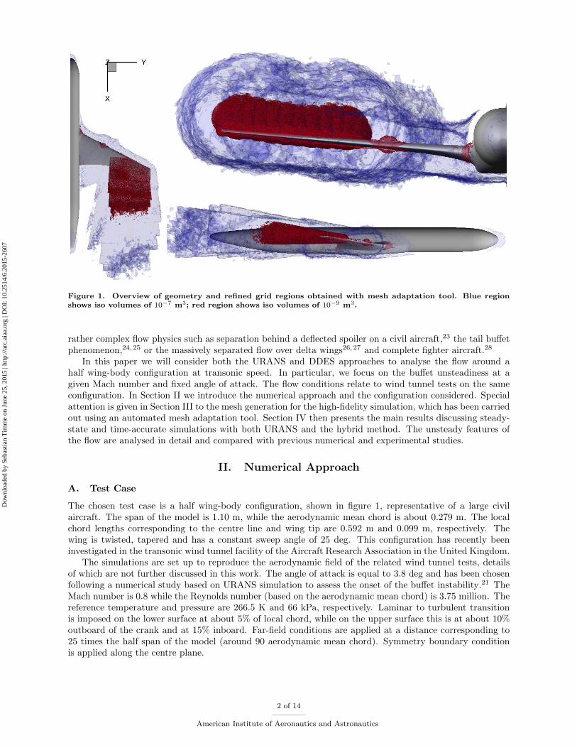
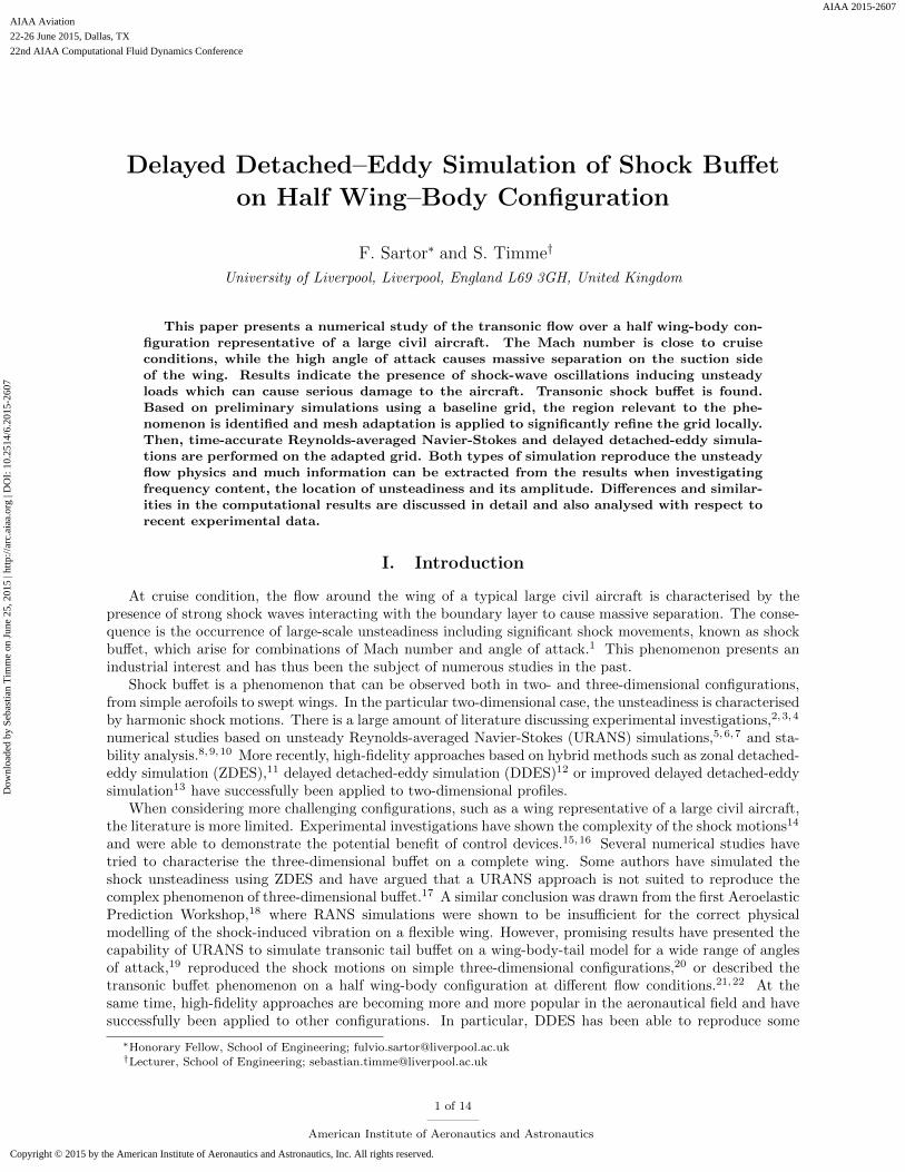
Figure 1. Overview of geometry and refined grid regions obtained with mesh adaptation tool. Blue regionshows iso volumes of 10−7 m3; red region shows iso volumes of 10−9 m3.

rather complex flow physics such as separation behind a deflected spoiler on a civil aircraft,23 the tail buffetphenomenon,24,25 or the massively separated flow over delta wings26,27 and complete fighter aircraft.28

In this paper we will consider both the URANS and DDES approaches to analyse the flow around ahalf wing-body configuration at transonic speed. In particular, we focus on the buffet unsteadiness at agiven Mach number and fixed angle of attack. The flow conditions relate to wind tunnel tests on the sameconfiguration. In Section II we introduce the numerical approach and the configuration considered. Specialattention is given in Section III to the mesh generation for the high-fidelity simulation, which has been carriedout using an automated mesh adaptation tool. Section IV then presents the main results discussing steady-state and time-accurate simulations with both URANS and the hybrid method. The unsteady features ofthe flow are analysed in detail and compared with previous numerical and experimental studies.

II. Numerical Approach

A. Test Case

The chosen test case is a half wing-body configuration, shown in figure 1, representative of a large civilaircraft. The span of the model is 1.10 m, while the aerodynamic mean chord is about 0.279 m. The localchord lengths corresponding to the centre line and wing tip are 0.592 m and 0.099 m, respectively. Thewing is twisted, tapered and has a constant sweep angle of 25 deg. This configuration has recently beeninvestigated in the transonic wind tunnel facility of the Aircraft Research Association in the United Kingdom.

The simulations are set up to reproduce the aerodynamic field of the related wind tunnel tests, detailsof which are not further discussed in this work. The angle of attack is equal to 3.8 deg and has been chosenfollowing a numerical study based on URANS simulation to assess the onset of the buffet instability.21 TheMach number is 0.8 while the Reynolds number (based on the aerodynamic mean chord) is 3.75 million. Thereference temperature and pressure are 266.5 K and 66 kPa, respectively. Laminar to turbulent transitionis imposed on the lower surface at about 5% of local chord, while on the upper surface this is at about 10%outboard of the crank and at 15% inboard. Far-field conditions are applied at a distance corresponding to25 times the half span of the model (around 90 aerodynamic mean chord). Symmetry boundary conditionis applied along the centre plane.

2 of 14

American Institute of Aeronautics and Astronautics

Dow

nloa

ded

by S

ebas

tian

Tim

me

on J

une

25, 2

015

| http

://ar

c.ai

aa.o

rg |

DO

I: 1

0.25

14/6

.201

5-26

07

Number of cores

Sp

ee

d­u

p

0 500 1000 15000

10

20

30

40

50

60

Linear speed­up compared to 24 cores

Speed­up

74%

79%

77%

87%

74%

Figure 2. Scaling of DLR-TAU code on ARCHER using adapted mesh with 28.9 M points.

B. Flow Solver

The simulations were performed using the unstructured finite volume solver TAU, developed by the GermanAerospace Center (DLR) and widely used in the European aerospace sector. The turbulence model usedin the URANS simulation is the negative Spalart-Allmaras (SA) model.29 Concerning the scale-resolvingapproach, the flow is investigated using DDES30 with the original SA turbulence model.31 Delayed DES is animproved version of the original formulation32 in terms of preventing the switching to large-eddy simulation(LES) inside boundary layers. A more complete review of this family of scale-resolving simulations, theirweaknesses and application can be found in [33].

In the URANS simulation, the second-order central scheme with scalar dissipation was used for theconvective fluxes of the Navier-Stokes equations, while a first-order Roe scheme was employed for those ofthe turbulence model. For DDES, a low dissipative, second-order central scheme with matrix dissipationwas chosen for the convective fluxes of the Navier-Stokes and turbulence equations. Gradients of the flowvariables, used for the diffusive and source terms, are reconstructed using the Green-Gauss theorem.

While fine-tuning the solver settings for DDES and URANS, it quickly became clear that an optimalsetting for DDES is not necessarily suited for the URANS approach. Indeed such URANS simulations gaverather low-amplitude signals for both lift and drag coefficients, and even no buffet at all when using thesecond-order central scheme for the convective fluxes of the turbulence model. For DDES on the other hand,once a low dissipative setup for the fluxes of the Navier-Stokes equations was established, the choice of theturbulence model discretisation became a minor factor.

Time-accurate computations employ the standard second-order dual-time stepping approach. A dynamicCauchy convergence criterion is applied for iterations in dual-time. Each time step is iterated until the dragcoefficient, chosen as control variable, shows a relative error smaller than 10−8 in the last 20 inner iterations.A minimum of 80 and 100 inner iterations is always performed for URANS and DDES, respectively, regardlessof the drag convergence, while a maximum of 500 inner iterations is imposed when the convergence criterionis not reached before.

C. Resources and Performance

All simulations were run on ARCHERa, which at the time of writing was the United Kingdom’s primaryacademic research supercomputer. It is a facility built around a Cray XC30 supercomputer providing thecentral computational resource. For optimal performance the Zoltan library34 was linked to DLR-TAU toguarantee a proper partitioning of the adapted mesh. To perform scaling tests, the mesh was split into alarge number of domains for numbers of cores ranging from 24 to 1536. As shown in figure 2, the DLR-TAUcode performs reasonably well in the considered range giving a scalability of over 70% compared to 24 cores.The production job was then run on 960 cores, where the speed-up is around 80%.

aAdvanced Research Computing High End Resource.

3 of 14

American Institute of Aeronautics and Astronautics

Dow

nloa

ded

by S

ebas

tian

Tim

me

on J

une

25, 2

015

| http

://ar

c.ai

aa.o

rg |

DO

I: 1

0.25

14/6

.201

5-26

07

(a) Baseline grid: 8.1 M points and 17.4 M elements (b) First adaptation: 8.5 M points and 19.0 M elements

(c) Second adaptation: 9.5 M points and 24.9 M elements (d) Third adaptation: 12.7 M points and 43.5 M elements

Figure 3. Refinement of grid following adaptation and smoothing; slice at 73% span. The fourth adaptationstep gives the final mesh with 28.9 M points and 117.1 M elements.

III. Grid Adaptation

For scale-resolving simulations, a highly refined mesh is needed in order to resolve the small turbulentstructures present in the separated zone. For the current case, the massively separated flow represents onlya small portion of the flow field, so that a uniform refinement of the computational domain is not an efficientapproach. The Chimera technique was initially considered but then quickly discarded due to the rather poorperformance of the DLR-TAU code. The flow solver performs grid interpolation of the Chimera block at eachphysical time step even though the connectivity is not changing, thus slowing down the overall simulation.

Another important grid technology is adaptive mesh refinement, where the mesh is refined locally in agiven zone of the domain based on some specified criterion. This approach seems to be particularly wellsuited for DDES and has successfully been applied before.26 The main requirements of a local refinementstrategy are the detection of grid areas to be refined and the method of element subdivisions resultingfrom insertion of new points in the identified areas. The adaptation tool of DLR-TAU uses an edge basedapproach. This means that the refinement indicators are evaluated for all edges, new points are inserted atmid-points of selected edges and the element subdivisions are determined from the layout of refined edges.The refinement tool also includes surface approximation and reconstruction for curved surfaces when addingnew surface points, and modification of the first cell height (not used though to keep the normal wall-spacingconstant). Details of the numerical implementation of the grid refinement can be found in [35,36].

Due to the time-varying location of the massively separated zone in a buffet investigation, a large portionof the wing has been selected for refinement following a preliminary URANS simulation, which was run forseveral buffet periods at the same flow conditions using the baseline grid. This non-refined grid has previouslybeen created using the Solar grid generator37 and thoroughly analysed.21 The refinement region was thenselected in order to cover high values of the time-averaged eddy viscosity. Based on this information, twelvefrustums, as indicated in figure 1, are defined spanning the outer wing sections and wake. A representationof the refined zones is visible in the figure as well with the blue surfaces representing cell volumes equal to10−7 m3, while the red surfaces surround cells with volumes equal to 10−9 m3.

4 of 14

American Institute of Aeronautics and Astronautics

Dow

nloa

ded

by S

ebas

tian

Tim

me

on J

une

25, 2

015

| http

://ar

c.ai

aa.o

rg |

DO

I: 1

0.25

14/6

.201

5-26

07

(a) Convergence of density residual (b) Drag polars

Figure 4. Convergence of density residual and drag polars comparing first-order Roe and second-order centralconvective schemes for SA turbulence model.

(a) 1st order Roe scheme.2.4 deg angle of attack

(b) 2nd order central scheme.2.4 deg angle of attack

(c) 1st order Roe scheme.3.8 deg angle of attack

(d) 2nd order central scheme.3.8 deg angle of attack

Figure 5. Surface-pressure distribution and separation line following steady state simulation.

Four steps are needed to obtain the refined grid starting from the baseline version. During each adaptationiteration, only those cells with edges larger than a given value are refined. This value decreases while iteratingthe adaptation in order to have a gradual refinement. Hexahedral cells in the boundary layer over the wingare also refined in this process to avoid discontinuities in grid spacing towards the surrounding tetrahedralzone. Note that the first three steps are mostly done to obtain a fairly smooth zone in the wake region, whilethe last step, which is the most expensive to compute, will create the final resolved zone. Grid-smoothingis applied after each adaptation step to obtain a more homogeneous overall spacing. A slice of the domainshowing the grid-spacing modification after the first three steps is given in figure 3. The result after thelast adaptation step is not included in the figure due to its fineness. The final grid, which is then used forboth URANS and DDES investigations, is composed of 28.9 M points and 117.1 M elements. The completeadaptation process can be run in a few hours on a modern workstation.

5 of 14

American Institute of Aeronautics and Astronautics

Dow

nloa

ded

by S

ebas

tian

Tim

me

on J

une

25, 2

015

| http

://ar

c.ai

aa.o

rg |

DO

I: 1

0.25

14/6

.201

5-26

07

Figure 6. Overview of DDES showing iso contours of Q-criterion at dimensionless value 100.

IV. Results

A. Steady-State Simulations

Reynolds-averaged Navier-Stokes simulations are first performed to converge the governing equations andthe results are presented in figures 4 and 5. Simulations at several angles of attack are considered usinga first-order Roe and a second-order central scheme for the convective terms of the turbulence model. Infigure 4a the evolution of the final density residual normalised by the initial value is plotted over the angle ofattack. Focussing on the results obtained with the Roe scheme, when the incidence is smaller than 3.0 deg,the results present a good level of convergence. After this threshold, the final residual rises and the simulationfails to converge to the specified limit. In the case of the central scheme however, the RANS simulationsconverge towards a steady state regardless, suggesting a failure of the simulation to predict the presence ofmassively separated flow. The same problem with the central scheme is also encountered when consideringtime-accurate RANS simulations, but not when using DDES. Figure 4b presents the corresponding dragpolar for the steady-state solutions obtained with the two numerical schemes. The agreement is perfect forsmall angles of attack, while discrepancies are observed once strong shock-wave/boundary-layer interactionis present eventually leading to the shock buffet unsteadiness.

The same behaviour is also found in figure 5, showing the pressure distribution on the surface of thewing. The solid black lines indicate the location of the separated zone by a change in sign of the skinfriction coefficient. When considering smaller angles of attack, the solutions are very similar as can be seenin figures 5a and 5b, whereas for higher angles the separated zones differ significantly. The results usingthe Roe scheme seem to be more reliable since unsteady simulations confirm that the flow field is indeedunsteady. In this case the separated zone is split and the shock foot lays on a curved line, as observed in aprevious study.21 It should be kept in mind however, since the solution presents massively separated zonesfor high angles of attack, time-accurate simulations should be considered instead to investigate the presenceof unsteady flow features.

B. Time-Accurate Simulations

The RANS simulations at 3.8 deg angle of attack are used as starting point for the time-accurate simulations.Once a (partially) converged flow field is obtained, the time discretisation is switched to dual-time stepping

6 of 14

American Institute of Aeronautics and Astronautics

Dow

nloa

ded

by S

ebas

tian

Tim

me

on J

une

25, 2

015

| http

://ar

c.ai

aa.o

rg |

DO

I: 1

0.25

14/6

.201

5-26

07

Figure 7. Perspective of DDES showing iso contours of Q-criterion at dimensionless value 100.

with the physical time-step size set to 1 µs. Considering the ratio between a characteristic length (i.e. theaerodynamic mean chord) and a characteristic (i.e. reference) velocity, a convective time typical for thesimulation can be defined. In this case the convective time is around 10−3 s which is significantly higherthan the chosen physical time-step size. The total physical time simulated is 0.1 s, corresponding to about20 to 30 buffet cycles. A transient part can be observed when the flow develops the unsteadiness. Once thistransient has passed, time histories of force and moment coefficients are recorded, and then power spectraldensity of these signals are analysed for the frequency content of the unsteadiness. Mean and variance of allflow variables are calculated as well; a functionality readily available in the DLR-TAU code.

Figures 6 and 7 show instantaneous iso contours of the Q-criterion at a dimensionless value 100 fromdifferent perspectives. The iso contours are coloured by the vertical velocity component, while the wing-fuselage geometry is coloured by the surface pressure distribution. In addition, streamlines coloured byvelocity magnitude and contour lines of Mach number are presented in figure 7. The Mach number contoursat five span-wise stations indicate the extent of the supersonic region on the suction side of the wing.

Turbulent structures are shed away from the shock foot, which has moved upstream due to the presence ofthe separated zone. Two separated zones are visible on the wing, each of them responsible for the turbulentstructures represented by the Q-criterion. It can be observed that the shock-induced separation, besidescausing the presence of the turbulent structures, is responsible for the pressure drop at the trailing edge.The pressure drop causes a decrease in the lift coefficient while increasing the drag. During a buffet cycle,the separated zone moves from the inboard to the outboard portion of the wing, causing periodic variationof forces and moments on the wing. The wing-tip vortex is also visible in the figures through the Q-criterion.Its downstream extent coincides with the highly-refined grid region, as shown in figure 1.

Time histories of the lift and drag coefficients are presented in figure 8. The plot compares the twosimulations on the adapted grid with the result obtained in [21] using the baseline non-adapted grid at thesame flow conditions. Focussing on the two URANS simulations, it can be seen that the presence of thegrid refinement has an impact on the evolution of the forces. However, the average values, the amplitudesof the fluctuations, and the frequency content of the shock motions remain very similar. Looking at thetime histories of the forces obtained using DDES, some differences can be noticed. The forces predicted bythe URANS approach are higher, which is particularly visible for the lift coefficient presented in figure 8a.Nevertheless, especially when comparing the drag coefficient as shown in figure 8b, the agreement is satisfying.From both figures it is also clear that the high-fidelity approach needs a longer transient to develop the fullyestablished regime, and a longer overall simulation must be considered.

7 of 14

American Institute of Aeronautics and Astronautics

Dow

nloa

ded

by S

ebas

tian

Tim

me

on J

une

25, 2

015

| http

://ar

c.ai

aa.o

rg |

DO

I: 1

0.25

14/6

.201

5-26

07

(a) Lift coefficient (b) Drag coefficient

Figure 8. Time histories of lift and drag coefficients obtained from different simulations.

frequency in Hertz

log

10

(p

ow

er

sp

ectr

al d

ensity)

101

102

103

104­15

­10

­5

0

URANS: baseline

URANS: adapted

DDES

(a) Lift coefficient

frequency in Hertz

log

10

(p

ow

er

sp

ectr

al d

ensity)

101

102

103

104­15

­10

­5

0

URANS: baseline

URANS: adapted

DDES

(b) Drag coefficient

Figure 9. Power spectral density of lift and drag coefficients obtained from different simulations.

Both simulation approaches can predict transonic buffet, characterised by non-periodic shock motions.These results are compatible with those obtained, on a different configuration, in [17] by means of ZDES.The signals obtained with a URANS approach are less rich in high-frequency fluctuations, probably due tothe lack of resolved turbulent content.

Table 1 gives an overview of the average values and standard deviations of the lift and drag coefficientsobtained with the different simulation approaches. The statistics are based on a signal of 0.07 s, excludingthe transient part of the simulation. The overall grid dependency is limited, since the mesh refinement doesnot seem to impact the URANS results significantly. The relative error of the average values is less than0.2% for both lift and drag coefficients. The DDES approach predicts smaller quantities for both lift anddrag coefficient, roughly 2% smaller than the URANS approach. Looking at the standard deviations, similarvalues can be found in all cases.

The frequency content of the shock motions is now discussed by analysing the power spectral density(PSD) of the lift and drag coefficient fluctuations. As pointed out in [38], numerical signals issued from CFD

8 of 14

American Institute of Aeronautics and Astronautics

Dow

nloa

ded

by S

ebas

tian

Tim

me

on J

une

25, 2

015

| http

://ar

c.ai

aa.o

rg |

DO

I: 1

0.25

14/6

.201

5-26

07

Table 1. Mean and standard deviation of lift and drag coefficients.

mean lift SD lift mean drag SD drag

URANS baseline 0.6376 5.328E-03 0.0494 4.300E-04

URANS adapted 0.6367 4.942E-03 0.0491 3.027E-04

DDES 0.6249 5.010E-03 0.0486 5.069E-04

(a) Mean values (b) Instantaneous at time 0.1 s

Figure 10. Instantaneous and mean surface pressure with slices of delay switch function fd showing (1 − fd).

are often oversampled and have a short duration. This can cause a problem since the spectrum definitionis linked to the signal length. The solution adopted to overcome this problem is to use an autoregressiveestimator,39 rather than a traditional Fast Fourier Transform. In particular, following the steps outlinedin [11], the autoregressive PSD is computed using Burg’s (or maximum entropy) method.40 Each case isanalysed using a single window covering the total duration of the signals, without the initial transient. Theorder of the autoregressive model has been set to 5000 after a parametric study, and is the same for allconsidered cases.

The results of the PSD thus obtained are presented in figure 9. As for figure 8, the plot includes forcomparison also the results obtained using the baseline grid. Very similar conclusions can be drawn analysingeither the lift or drag coefficient in figures 9a and 9b, respectively. For all cases, a low-frequency peak canbe observed. The peak is broadband, indicating that the shock unsteadiness is characterised by non-periodicmotions. Good agreement can be found between the URANS simulations on the baseline and the adaptedgrid, reconfirming the low impact of the grid refinement on the flow physics. Comparing the PSD of theDDES signals to URANS, the main peak occurs at a slightly lower frequency, indicating that the high-fidelityapproach predicts buffet with a longer period. All signals analysed agree on the shock motions occurringat a broadband frequency range between 150 and 300 Hz. This corresponds, once scaled using the non-dimensional time given by the ratio of aerodynamic mean chord and reference velocity, to a Strouhal numberof about 0.15 to 0.3. Here again the spectrum is fairly similar to the results obtained in [17] by means ofZDES, without any significant peak in the high-frequency content.

Figure 10 presents instantaneous and mean values of surface pressures and slices of the delay switchfunction of the DDES formulation called fd. The plot is showing (1− fd) with values close to one indicatingRANS mode, whereas values close to zero indicate LES mode. Focussing on the inboard part of the wing,the mean values, presented in figure 10a, equal the instantaneous values, presented in figure 10b. In thisregion the shielding always gives RANS mode because neither the mesh nor the physics allow it differently.Focussing outboard of the crank, instantaneous changes are clearly visible. In this region the refined part ofthe mesh is located, and turbulent structures are resolved where significant separation occurs. During grid

9 of 14

American Institute of Aeronautics and Astronautics

Dow

nloa

ded

by S

ebas

tian

Tim

me

on J

une

25, 2

015

| http

://ar

c.ai

aa.o

rg |

DO

I: 1

0.25

14/6

.201

5-26

07

(a) URANS (b) DDES

Figure 11. Instantaneous values of eddy-viscosity ratio.

adaptation, about 21 M points were added in the outboard region of the wing where separation is found.The percentage of grid points which are treated in LES mode has been monitored and the value is alwaysabout 70%. This number slightly varies in time, since during the buffet cycle intermittent boundary layerseparation and re-attachment occurs. For instance, when the shock is in its most downstream position, noseparation can be found in the refined region. Even if the grid spacing allows an LES treatment, the delayswitch is not active.

A consequence of the LES treatment in the separated region can be seen from the instantaneous eddy-viscosity ratio, shown in figure 11. The ratio of turbulent (i.e. eddy) viscosity to laminar viscosity is presented.Considering the URANS simulation in figure 11a, the turbulence content is modelled in the entire domain.Very high values of eddy viscosity are clearly visible in the wake of the separated region. More specifically,a blob of eddy viscosity is always present in the wake of the wing region where separation occurs. Since thisregion varies in time and moves along the wing span periodically, regions with high values of eddy viscositycan also be seen periodically downstream of the wing. Considering an equivalent plot for DDES in figure 11bon the other hand, the simulated part of turbulence is predominant, while the modelled part only causessmall values of eddy-viscosity. (Note the scale changes between the two plots.) However, the turbulencecontent is still modelled in the inboard part of the wing, where the grid spacing does not allow to resolvethe detached eddies downstream of the trailing edge. This should not have an influence on the descriptionof the buffet phenomenon, which concerns only the outer part of the wing.

Figure 12 presents the average spatial distribution of the pressure, evaluated at the surface of the wing.The numerical results obtained with URANS and DDES are also compared with a result of the experimentalinvestigation performed in the transonic wind tunnel of the Aircraft Research Association in the UnitedKingdom using unsteady pressure-sensitive paint. The flow conditions are a Mach number of 0.80 and4.6 deg angle of attack. The higher experimental angle of attack yields a lift coefficient of 0.625, which isclosest to the case considered in the numerical investigation. Note that the computations presented in thiswork have been performed considering a rigid model, without taking into account the static deformation ofthe wing in the wind tunnel. Part of the disagreement between the experimental data and the numericalresults is due to this approximation.

Comparing DDES and URANS results, excellent agreement can be observed in terms of shock positioninboard of the crank. Then, upstream of the separated zone outboard of the crank, a small differenceis present. In figure 12a the mean shock foot trace predicted by the URANS approach is more bent incomparison. The DDES results in figure 12b are in better agreement with the experimental investigation.However, comparing the pressure drop at the trailing edge due to the separated zone, the URANS resultsare in closer agreement with the experiments, while DDES predicts a pressure drop covering a wider part

10 of 14

American Institute of Aeronautics and Astronautics

Dow

nloa

ded

by S

ebas

tian

Tim

me

on J

une

25, 2

015

| http

://ar

c.ai

aa.o

rg |

DO

I: 1

0.25

14/6

.201

5-26

07

(a) URANS (b) DDES (c) Experimental data

Figure 12. Mean surface-pressure distributions.

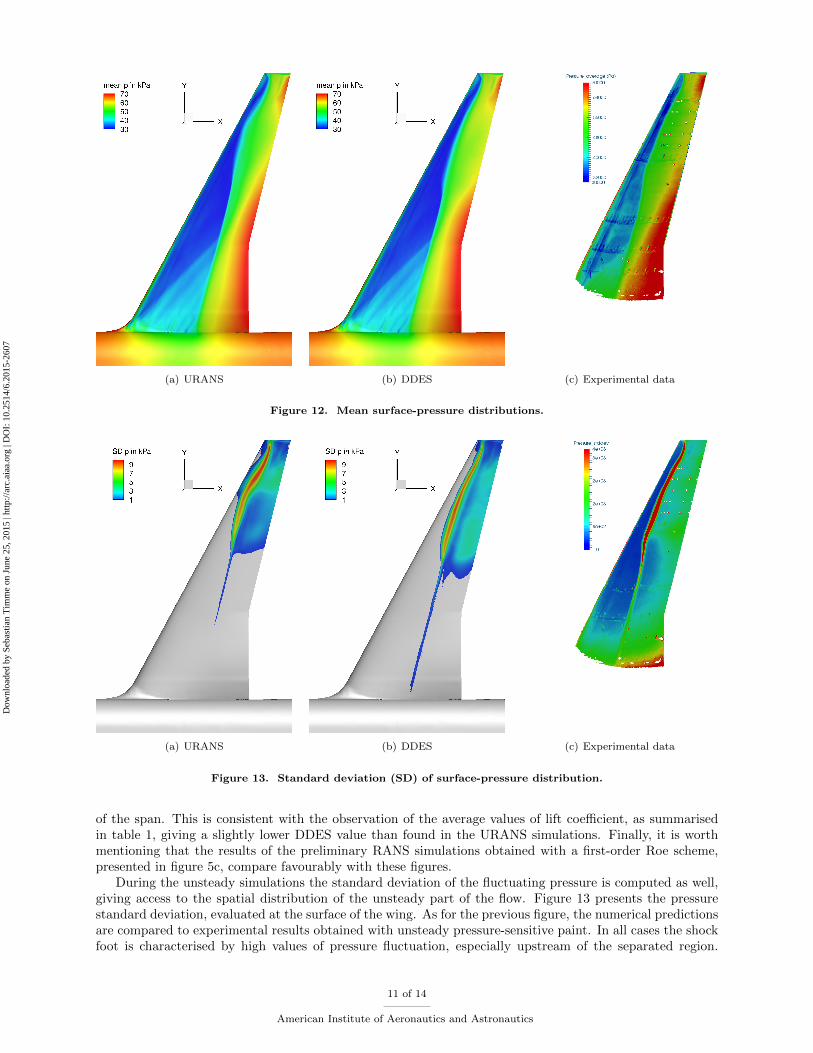
(a) URANS (b) DDES (c) Experimental data

Figure 13. Standard deviation (SD) of surface-pressure distribution.

of the span. This is consistent with the observation of the average values of lift coefficient, as summarisedin table 1, giving a slightly lower DDES value than found in the URANS simulations. Finally, it is worthmentioning that the results of the preliminary RANS simulations obtained with a first-order Roe scheme,presented in figure 5c, compare favourably with these figures.

During the unsteady simulations the standard deviation of the fluctuating pressure is computed as well,giving access to the spatial distribution of the unsteady part of the flow. Figure 13 presents the pressurestandard deviation, evaluated at the surface of the wing. As for the previous figure, the numerical predictionsare compared to experimental results obtained with unsteady pressure-sensitive paint. In all cases the shockfoot is characterised by high values of pressure fluctuation, especially upstream of the separated region.

11 of 14

American Institute of Aeronautics and Astronautics

Dow

nloa

ded

by S

ebas

tian

Tim

me

on J

une

25, 2

015

| http

://ar

c.ai

aa.o

rg |

DO

I: 1

0.25

14/6

.201

5-26

07

(a) Slice parallel to outer wing trailing edge (b) Slice at 73% span

Figure 14. Instantaneous divergence of velocity field at time 0.092 s showing pressure waves generated by theseparated zone.

However, the unsteadiness is also inboard of the crank. Figures 13a and 13b indicate that the entire shockfoot is unsteady, regardless the presence of downstream separation. The bulk of the unsteadiness lays on abent line for both numerical and experimental results. A very similar shock-foot trace has been observed inprevious studies on a wing with a different planform17 and on a infinite-swept configuration.20 The mainconsequence is that the distance between the shock foot and the trailing edge is not constant along the wingspan. This feature has been linked to the buffet frequency in a previous work.21

Only for the URANS simulation, presented in figure 13a, high pressure fluctuations are visible even nearthe leading edge, especially close to the wing tip. This feature is neither present in the DDES results northe experimental data in figures 13b and 13c. However, a leading edge without pressure fluctuations hasbeen observed in URANS simulations when considering different angles of attack21 or Mach numbers.22

Concerning the experimental result of figure 13c, the unsteady shock pattern appears to be much closer toDDES than URANS simulations. Also, the unsteadiness in the separated region downstream of the shockfoot agrees closer to DDES. The slightly increased levels of pressure variance near the wing-root trailing edgeis an systematic experimental error due to variations in intensity reflected by the pressure-sensitive paint.

The interaction between large-scale turbulent structures and the trailing edge causes acoustic radiation.Figure 14 shows an instantaneous divergence of the velocity field to illustrate such pressure waves as previ-ously observed by means of ZDES in [11] in the flow around a supercritical aerofoil. In particular, figure 14apresents a slice downstream and parallel to the trailing edge on the outer part of the wing highlighting thepresence of pressure waves generated by the separated zone and propagating away from the source. Up-stream travelling disturbances originating at the trailing edge are visible in the slice at 73% span shown infigure 14b. Note that the solid black line included on the surface of the wing in figure 14a describes thelocation of the slice at 73% span.

As pointed out in [17] for another half wing-body configuration, the propagation process is a three-dimensional phenomenon. This can be seen in figure 14 from both the stream-wise and span-wise propagatingwaves affecting the dynamics of the shock motion and separation line. The propagating waves can thusgenerate a feedback mechanism, as proposed in [41] for the two-dimensional case, which must be thenbe extended to the three-dimensional situation. In a recent paper it was argued that the reason for thebroadband-frequency nature of three-dimensional buffet (rather than distinct periodic shock motions) has tobe sought in the three-dimensionality of the shock pattern.21 Unlike the two-dimensional case, the stream-wise distance travelled by the acoustic waves before hitting the shock is not constant along the span of athree-dimensional wing. Thus, the buffet phenomenon is not characterised by perfectly periodic motions.These conclusions will be investigated further.

12 of 14

American Institute of Aeronautics and Astronautics

Dow

nloa

ded

by S

ebas

tian

Tim

me

on J

une

25, 2

015

| http

://ar

c.ai

aa.o

rg |

DO

I: 1

0.25

14/6

.201

5-26

07

V. Conclusions

The aim of the present work is to analyse the flow over a large civil aircraft at cruise conditions. At afixed Mach number the angle of attack is increased until a massively separated region appears on the suctionside of the wing. Unsteady flow, known as transonic buffet, is observed. A standard URANS simulation isfirst conducted on a baseline grid, and it is shown to be capable of reproducing the typical shock motions.Mesh adaptation is then considered to refine the grid in the region of the computational domain relevantto the unsteadiness. Using the highly refined grid, both URANS and DDES approaches are investigatedto predict the shock buffet phenomenon. Results of the simulations are presented with particular focus onthose of the high-fidelity hybrid approach.

Concerning the shock unsteadiness, the lift fluctuations show that, unlike the two-dimensional case, theunsteadiness is not limited to a periodic oscillation. The unsteady separated zone extends from the wing tipto the crank, and shock motions influence the flow over the entire wing. The frequency content of the liftfluctuations indicates that shock motions occur at frequencies between 150 and 300 Hz. The results agreewith conclusions drawn from previous experimental and numerical shock buffet investigations.

In general, the shock unsteadiness appears at time scales which are much longer than those of thewall-bounded turbulence. Thus, a numerical simulation solving the RANS equations in a time-accuratemanner closed with a turbulence model is justified. Such unsteady RANS simulations are capable to predict,within the limits of a RANS approach, the main features of the flow. However, the results obtained fromDDES provide a more thorough description of the flow physics involved in the buffet phenomenon. Aqualitative comparison between simulation results and experimental data indicates closer agreement for thescale-resolved simulation.

Acknowledgements

The authors are grateful to Simon Lawson from Aircraft Research Association for the inspection of thewind tunnel model and for providing the experimental data. The authors wish also to acknowledge MarcoHahn from the same organisation for generating the baseline meshes. The research leading to these resultshas received funding from the European Union’s Seventh Framework Programme (FP7/2007-2013) for theClean Sky Joint Technology Initiative under grant agreement n◦336948. This work used the ARCHER UKNational Supercomputing Service (http://www.archer.ac.uk).

References

1Lee, B. H. K., “Self-sustained shock oscillations on airfoils at transonic speeds,” Progress in Aerospace Sciences, Vol. 37,No. 2, 2001, pp. 147–196.

2McDevitt, J. B., Levy, J. L. L., and Deiwert, G. S., “Transonic flow about a thick circular-arc airfoil,” AIAA Journal ,Vol. 14, No. 5, 1976, pp. 606–613.

3McDevitt, J. B. and Okuno, A. F., “Static and dynamic pressure measurements on a NACA 0012 airfoil in the Ameshigh Reynolds number facility,” NASA TP-2485 , 1985.

4Jacquin, L., Molton, P., Deck, S., Maury, B., and Soulevant, D., “Experimental study of shock oscillation over a transonicsupercritical profile,” AIAA Journal , Vol. 47, No. 9, 2009, pp. 1985–1994.

5Barakos, G. and Drikakis, D., “Numerical simulation of transonic buffet flows using various turbulence closures,” Inter-national Journal of Heat and Fluid Flow , Vol. 21, No. 5, 2000, pp. 620–626.

6Goncalves, E. and Houdeville, R., “Turbulence model and numerical scheme assessment for buffet computations,” Inter-national Journal for Numerical Methods in Fluids, Vol. 46, No. 11, 2004, pp. 1127–1152.

7Thiery, M. and Coustols, E., “Numerical prediction of shock induced oscillations over a 2D airfoil: Influence of turbulencemodelling and test section walls,” International Journal of Heat and Fluid Flow , Vol. 27, No. 4, 2006, pp. 661–670.

8Crouch, J. D., Garbaruk, A., Magidov, D., and Travin, A., “Origin of transonic buffet on aerofoils,” Journal of FluidMechanics, Vol. 628, 2009, pp. 357–369.

9Sartor, F., Mettot, C., and Sipp, D., “Stability, receptivity and sensitivity analyses of buffeting transonic flow over aprofile,” AIAA Journal , 2014, pp. 1–14.

10Iorio, M. C., Gonzalez, L. M., and Ferrer, E., “Direct and adjoint global stability analysis of turbulent transonic flowsover a NACA0012 profile,” International Journal for Numerical Methods in Fluids, Vol. 76, No. 3, 2014, pp. 147–168.

11Deck, S., “Numerical simulation of transonic buffet over the OAT15A airfoil,” AIAA Journal , Vol. 43, No. 7, 2005,pp. 1556–1566.

12Grossi, F., Braza, M., and Hoarau, Y., “Prediction of Transonic Buffet by Delayed Detached-Eddy Simulation,” AIAAJournal , 2014, pp. 1–13.

13 of 14

American Institute of Aeronautics and Astronautics

Dow

nloa

ded

by S

ebas

tian

Tim

me

on J

une

25, 2

015

| http

://ar

c.ai

aa.o

rg |

DO

I: 1

0.25

14/6

.201

5-26

07

13Huang, J., Xiao, Z., Liu, J., and Fu, S., “Simulation of shock wave buffet and its suppression on an OAT15A supercriticalairfoil by IDDES,” Science China Physics, Mechanics and Astronomy, Vol. 55, No. 2, 2012, pp. 260–271.

14Merienne, M.-C., Sant, Y. L., Lebrun, F., Deleglise, B., and Sonnet, D., “Transonic buffeting investigation using unsteadypressure-sensitive-paint in a large wind tunnel,” AIAA Paper 2013–1136 , 2013.

15Dandois, J., Molton, P., Lepage, A., Geeraert, A., Brunet, V., Dor, J.-B., and Coustols, E., “Buffet Characterisation andControl for Turbulent Wings,” Aerospace Lab, Vol. 6, 2013.

16Sugioka, Y., Numata, D., Asai, K., Koike, S., Nakakita, K., and Koga, S., “Unsteady PSP Measurement of TransonicBuffet on a Wing,” AIAA Paper 2015–0025 , 2015.

17Brunet, V. and Deck, S., “Zonal-detached eddy simulation of transonic buffet on a civil aircraft type configuration,”AIAA Paper 2008–4152 , 2008.

18Dalenbring, M., Jirasek, A., Heeg, J., and Chwalowski, P., “Initial Investigation of the Benchmark SuperCritical WingConfiguration using Hybrid RANS-LES modeling,” AIAA Paper 2013–1799 , 2013.

19Illi, S. A., Fingskes, C., Lutz, T., and Kramer, E., “Transonic Tail Buffet Simulations for the Common Research Model,”AIAA Paper 2013–2510 , 2013.

20Iovnovich, M. and Raveh, D. E., “Numerical Study of Shock Buffet on Three-Dimensional Wings,” AIAA Journal ,Vol. 53, No. 2, 2015, pp. 449–463.

21Sartor, F. and Timme, S., “Reynolds-Averaged Navier-Stokes Simulations of Shock Buffet on Half Wing-Body Configu-ration,” AIAA Paper 2015-1939 , 2015.

22Sartor, F. and Timme, S., “Mach number effects on buffeting flow on a half wing-body configuration,” 50th 3AF Inter-national Conference on Applied Aerodynamics. Toulouse, France, 2015.

23Gand, F., “Zonal detached eddy simulation of a civil aircraft with a deflected spoiler,” AIAA Journal , Vol. 51, No. 3,2012, pp. 697–706.

24Morton, S., Cummings, R. M., and Kholodar, D. B., “High resolution turbulence treatment of F/A-18 tail buffet,”Journal of Aircraft , Vol. 44, No. 6, 2007, pp. 1769–1775.

25Illi, S. A., , Lutz, T., and Kramer, E., “Transonic Tail Buffet Simulations on the ATRA Research Aircraft,” ComputationalFlight Testing, Springer, 2013, pp. 273–287.

26Mitchell, A. M., Morton, S. A., Forsythe, J. R., and Cummings, R. M., “Analysis of delta-wing vortical substructuresusing detached-eddy simulation,” AIAA Journal , Vol. 44, No. 5, 2006, pp. 964–972.

27Morton, S., “Detached-eddy simulations of vortex breakdown over a 70-degree delta wing,” Journal of Aircraft , Vol. 46,No. 3, 2009, pp. 746–755.

28Morton, S. A., Forsythe, J. R., Squires, K. D., and Cummings, R. M., “Detached-eddy simulations of full aircraftexperiencing massively separated flows,” The 5th Asian Computational Fluid Dynamics Conference, 2003.

29Allmaras, S. R., Johnson, F. T., and Spalart, P. R., “Modifications and clarifications for the implementation of theSpalart-Allmaras turbulence model,” ICCFD7-1902, 7th International Conference on Computational Fluid Dynamics, BigIsland, Hawaii , 2012.

30Spalart, P. R., Deck, S., Shur, M. L., Squires, K. D., .Strelets, M. K., and Travin, A., “A new version of detached-eddy simulation, resistant to ambiguous grid densities,” Theoretical and computational fluid dynamics, Vol. 20, No. 3, 2006,pp. 181–195.

31Spalart, P. R. and Allmaras, S. R., “A one–equation turbulence model for aerodynamic flows,” AIAA Paper 92–0439 ,1992.

32Spalart, P. R., Jou, W. H., Strelets, M., and Allmaras, S. R., “Comments on the feasibility of LES for wings, and on ahybrid RANS/LES approach,” Advances in DNS/LES , Vol. 1, 1997, pp. 4–8.

33Spalart, P. R., “Detached-eddy simulation,” Annual Review of Fluid Mechanics, Vol. 41, 2009, pp. 181–202.34Boman, E. G., Catalyurek, U. V., Chevalier, C., and Devine, K. D., “The Zoltan and Isorropia Parallel Toolkits for

Combinatorial Scientific Computing: Partitioning, Ordering, and Coloring,” Scientific Programming, Vol. 20, No. 2, 2012,pp. 129–150.

35Alrutz, T. and Orlt, M., “Parallel dynamic grid refinement for industrial applications,” ECCOMAS CFD 2006: Proceed-ings of the European Conference on Computational Fluid Dynamics, Egmond aan Zee, The Netherlands, September 5-8, 2006 ,Delft University of Technology; European Community on Computational Methods in Applied Sciences (ECCOMAS), 2006.

36Alrutz, T. and Vollmer, D., “Recent Developments of TAU Adaptation Capability,” MEGADESIGN and MegaOpt-German Initiatives for Aerodynamic Simulation and Optimization in Aircraft Design, Springer, 2009, pp. 3–19.

37Martineau, D. G., Stokes, S., Munday, S. J., Jackson, A. P., Gribben, B. J., and Verhoeven, N., “Anisotropic hybridmesh generation for industrial RANS applications,” AIAA Paper 2006-534 , 2006.

38Deck, S. and Nguyen, A. T., “Unsteady side loads in a thrust-optimized contour nozzle at hysteresis regime,” AIAAJournal , Vol. 42, No. 9, 2004, pp. 1878–1888.

39Kay, S. M. and Marple, S. L. J., “Spectrum analysis – a modern perspective,” Proceedings of the IEEE , Vol. 69, No. 11,1981, pp. 1380–1419.

40Burg, J. P., “Maximum entropy spectral analysis,” Modern Spectrum Analysis, Edited by D. G. Childers, IEEE Press,New York, 1978, pp. 34–41.

41Lee, B. H. K., “Oscillatory shock motion caused by transonic shock boundary-layer interaction,” AIAA Journal , Vol. 28,No. 5, 1990, pp. 942–944.

14 of 14

American Institute of Aeronautics and Astronautics

Dow

nloa

ded

by S

ebas

tian

Tim

me

on J

une

25, 2

015

| http

://ar

c.ai

aa.o

rg |

DO

I: 1

0.25

14/6

.201

5-26

07