Kennesaw State University Kennesaw State University

DigitalCommons@Kennesaw State University DigitalCommons@Kennesaw State University

Senior Design Project For Engineers Southern Polytechnic College of Engineering and Engineering Technology

Spring 4-28-2021

Delivery Route Optimization Delivery Route Optimization

Adam Esasky Kennesaw State University

Mark Iltsenko Kennesaw State University

Sean Jones Kennesaw State University

Matthew Tharakan Kennesaw State University

Follow this and additional works at: https://digitalcommons.kennesaw.edu/egr_srdsn

Part of the Engineering Commons

Recommended Citation Recommended Citation Esasky, Adam; Iltsenko, Mark; Jones, Sean; and Tharakan, Matthew, "Delivery Route Optimization" (2021). Senior Design Project For Engineers. 51. https://digitalcommons.kennesaw.edu/egr_srdsn/51

This Senior Design is brought to you for free and open access by the Southern Polytechnic College of Engineering and Engineering Technology at DigitalCommons@Kennesaw State University. It has been accepted for inclusion in Senior Design Project For Engineers by an authorized administrator of DigitalCommons@Kennesaw State University. For more information, please contact digitalcommons@kennesaw.edu.

Delivery Route Optimization

Team Drive Fast

Adam Esasky (Project Manager)

Matthew Tharakan (Field Expert)

Mark Iltsenko (Financial Officer)

Sean Jones (Technical Expert)

ISYE 4900 | Dr. Adeel Khalid

Kennesaw State University

April 28, 2021

Executive Summary

“The Carrier Company” is a service that delivers motorcycle parts all over South East,

US. They have over 38 routes that each have a driver designated to deliver products to their

clients twice a day. The majority of the company’s time and expenses are focused on the delivery

of the products to their respected clients. Recently, due to COVID-19, the Carrier Company has

had a number of issues with new drivers not knowing the routes and in turn taking too long to

deliver the products. The delay in delivery has caused a loss in profits for the Carrier Company

as they ae having to pay their drivers for more hours, their vehicles are racking up more mileage,

and their customers are becoming less satisfied with the delivery service. As a result, the Carrier

Company has asked Team Dive Fast to work on developing a program that optimizes the

delivery of products on a certain route to see if shortening the delivery time will have any effect

on company costs. After reviewing the problem, the team decided to pursue possible solution

options and came up with three possible options: A VRP (Vehicle Routing Problem), a TSP

(Traveling Salesman Problem), and a TDP (Truck Dispatching Problem). The team concluded

that the problem at hand was a TSP (Traveling Salesman Problem) and needed to be solved

accordingly due to their being only one driver and he would be delivering the whole route on his

own.

The program that was built takes the fastest route from the Distribution Center to all of

the expecting clients and computes the most optimal order to deliver the products. The program

also has alternative solutions that it computes to account for traffic, construction, natural

disasters, or any other types of emergencies that may delay the expected delivery times. A cost

benefit analysis was done to compare the cost effectiveness of the new program versus the

previous method. In total, the new program would save over $5,000 annually in company costs

for this route alone. The route that was selected for this program was the shortest and most

concise route that the company delivers to which would give us our lower limit for how much we

should expect to save if this program is applied to all 38 other routes. Taking the total annual

saving from this route and applying it to the other routes, The Carrier Company should expect to

see annual savings upwards of $200,000. By looking at these potential savings, our

recommendation to the Carrier Company would be to implement the new optimized program in

all of their delivery routes.

Table of Contents

Chapter 1: General Information..................................................................................................... 1

1.1 Introduction.......................................................................................................................1

1.2 Objective ...........................................................................................................................1

1.3 Justification .......................................................................................................................1

1.4 Project background ............................................................................................................2

1.5 Problem Statement ............................................................................................................2

Chapter 2: Literature ...................................................................................................................... 3

2.1 Literature Review ....................................................................................................................3

Chapter 3: Measurement .................................................................. Error! Bookmark not defined.

3.1 Problem Solving Approach .................................................................................................6

3.2 Requirements ....................................................................................................................6

3.3 Minimum Success Criteria ..................................................................................................7

3.4 Gantt Chart and Schedule...................................................................................................7

3.5 Flow Chart .........................................................................................................................8

3.6 Responsibilities ..................................................................................................................9

3.7 Budget ...............................................................................................................................9

3.8 Resources Used................................................................................................................ 10

Chapter 4: Solutions ..................................................................................................................... 11

4.1 Proposed Solutions .......................................................................................................... 11

4.2 Problem Definition........................................................................................................... 11

4.3 Solution Methods ............................................................................................................ 11

4.4 Making the Solution ......................................................................................................... 12

Chapter 5: Analysis ....................................................................................................................... 14

5.1 Verification Approach ...................................................................................................... 14

5.2 Time ................................................................................................................................ 14

5.3 Sensitivity Analysis........................................................................................................... 15

5.4 Distance Analysis ............................................................................................................. 17

5.5 Economic Analysis............................................................................................................ 18

Chapter 6: Results and Discussion ............................................................................................... 23

6.1 Summary of Analysis ........................................................................................................ 23

Chapter 7: Conclusion and Recommendations ............................................................................ 25

References .................................................................................................................................... 26

Appendix A: Acknowledgements ................................................................................................. 28

Appendix B: Contact Information ................................................................................................ 29

Appendix C: Reflections ................................................................................................................ 30

Appendix D: Contributions ........................................................................................................... 32

Appendix E: Additional Data ........................................................................................................ 34

List of Tables

Table 1: Budget .............................................................................................................................. 9

Table 2: TSP Solver ..................................................................................................................... 12

Table 3: Time Differences for 8 Stops......................................................................................... 14

Table 4: Route Order for Morning .............................................................................................. 15

Table 5: Average Travel Times .................................................................................................... 34

List of Figures

Figure 1: VRP ................................................................................................................................ 3

Figure 2: Problem Comparison ..................................................................................................... 4

Figure 3: Schedule ......................................................................................................................... 7

Figure 4: Delivery Flow Chart ...................................................................................................... 8

Figure 5: Solver Input ................................................................................................................. 13

Figure 6: Morning Route ............................................................................................................ 16

Figure 7: Afternoon Route .......................................................................................................... 16

Figure 8: Total Mileage ............................................................................................................... 17

Figure 9: Before Program Costs ................................................................................................. 18

Figure 10: After Program Costs .................................................................................................. 19

Figure 11: Company Costs .......................................................................................................... 20

Figure 12: Total Costs ................................................................................................................. 21

Figure 13: Optimal Route ............................................................................................................ 23

Figure 14: Unoptimized Route Visualization.............................................................................. 23

Figure 15: Optimized Route Visualization .................................................................................. 24

1

Chapter 1: General Information

1.1 Introduction

For the sake of the company’s business, their official name and their clients will not be listed or

called out, specifically in this report. The company will be referenced as the “Carrier Company”

and the clients will be numbered accordingly to allow for distinguishment in the results section.

The Carrier Company is a delivery service that caters to motorcycle body shops, repair shops,

and retailers where they deliver parts and products associated with all types of motorcycle

manufacturers across the country. The main scope of work for the Carrier Company is to take

products and parts from a manufacturer/distribution center and deliver those items to clients on a

bi-daily basis. The company is conducted of multiple drivers who handle routes that encompass

locations across the nation.

1.2 Objective

The objective of this project is to design and implement a program that will optimize the route

that drivers take to deliver their parts and products to their corresponding clients. By improving

and optimizing the route, the total cost to deliver an item should be lowered and the time it takes

to deliver an item should also be decreased. A decrease in time equates to a decrease in company

spending.

1.3 Justification

The carrier service has had numerous issues with driver spending to long delivering parts and in

turn it is costing them a great deal of money in labor over the course of a year. A more optimized

delivery route would help reduce travel time and ultimately save the company thousands of

dollars each year in delivering costs.

2

1.4 Project background

The Carrier Company does not have a specified and laid out plan as to how they deliver products

to their clients. The current method involves a driver typing in the address of the client into a

map search engine and then traveling to that location. Once the driver arrives at the first stop, the

driver then maps out the next delivery location and continues the same process until all of the

products are delivered to their respected locations. Due to ongoing circumstances that have arose

do to the COVID-19 outbreak, the Carrier has had to have a number of regular drivers miss work

and in turn be filled by new driver who are not familiar with the route. The result of these actions

has already caused issues such as new drivers taking a considerable amount of time longer to

deliver products. Which in turn, is delaying delivery times and resulting in a larger payout by the

Carrier Company as their drivers are paid by the hour and not by the service.

1.5 Problem Statement

The logistics of delivering products to their specified locations is an area where the Carrier

Company is having issues. With products being delayed and clients becoming less satisfied, a

solution to the problems is both important and imminent. Therefore, by minimizing the total

delivery times and shortening the routes, the Carrier Company will in turn make a greater

cumulative profit for the services that they provide to their clients.

3

Chapter 2: Literature

2.1 Literature Review

Regardless of what industry it is, delivery route optimization is one of the most common

problems that carrier companies face on a day-to-day basis. The ability to efficiently plan daily

routes with multiple stops can provide major cost and time savings. In this case, companies must

refer to route optimization. Which is defined as process of determining the most cost -efficient

route. In our case, we are trying to cut the total trip mileage, and improve time driver spends in

route. Solving this problem could potentially lower the cost of delivery as well as free up more

vehicles for additional routes. So far, there is a couple known approaches that has been widely

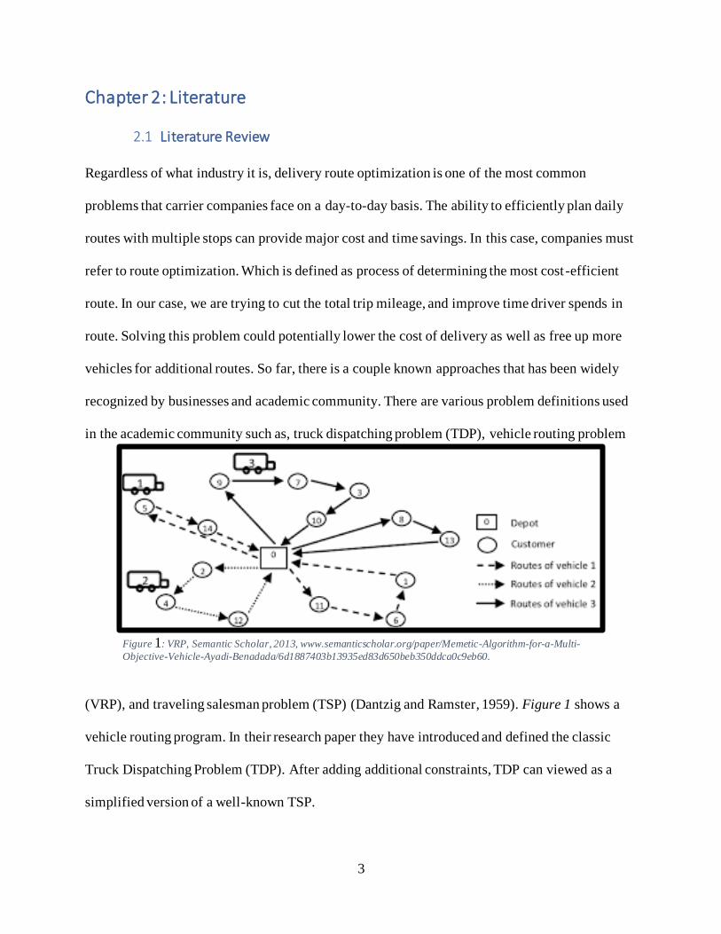
recognized by businesses and academic community. There are various problem definitions used

in the academic community such as, truck dispatching problem (TDP), vehicle routing problem

(VRP), and traveling salesman problem (TSP) (Dantzig and Ramster, 1959). Figure 1 shows a

vehicle routing program. In their research paper they have introduced and defined the classic

Truck Dispatching Problem (TDP). After adding additional constraints, TDP can viewed as a

simplified version of a well-known TSP.

Figure 1: VRP, Semantic Scholar, 2013, www.semanticscholar.org/paper/Memetic-Algorithm-for-a-Multi-

Objective-Vehicle-Ayadi-Benadada/6d1887403b13935ed83d650beb350ddca0c9eb60.

4

The TSP deals with identifying the shortest traveling route for a salesman to visit a given set of

customers. The TDP is different from TSP in the sense that after reaching m of the n customers,

the salesman has to return to the starting location. After that the salesman must start his next trip

visiting a new set of m customers. The TDP was later adjusted and generalized to VRP to

incorporate real world constraints and circumstances. (Schneider, Stenger, & Goeke, 2014).

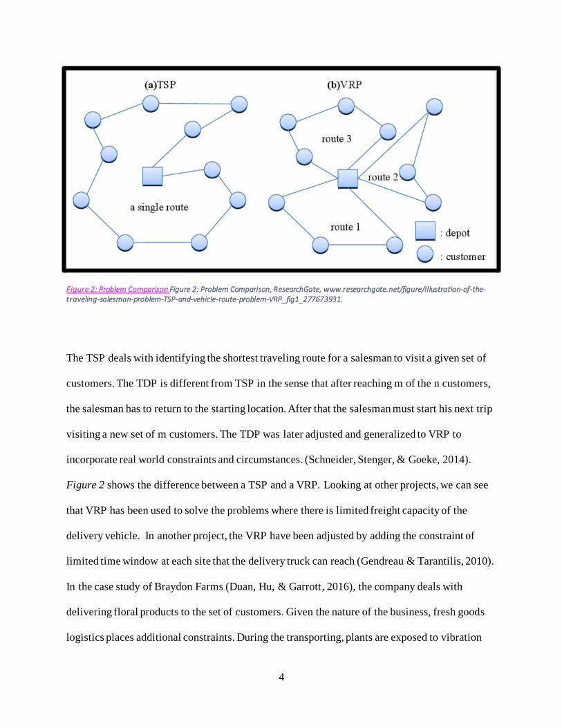
Figure 2 shows the difference between a TSP and a VRP. Looking at other projects, we can see

that VRP has been used to solve the problems where there is limited freight capacity of the

delivery vehicle. In another project, the VRP have been adjusted by adding the constraint of

limited time window at each site that the delivery truck can reach (Gendreau & Tarantilis, 2010).

In the case study of Braydon Farms (Duan, Hu, & Garrott, 2016), the company deals with

delivering floral products to the set of customers. Given the nature of the business, fresh goods

logistics places additional constraints. During the transporting, plants are exposed to vibration

Figure 2: Problem Comparison Figure 2: Problem Comparison, ResearchGate, www.researchgate.net/figure/Illustration-of-the-traveling-salesman-problem-TSP-and-vehicle-route-problem-VRP_fig1_277673931.

5

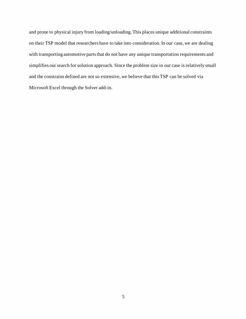
and prone to physical injury from loading/unloading. This places unique additional constraints

on their TSP model that researchers have to take into consideration. In our case, we are dealing

with transporting automotive parts that do not have any unique transportation requirements and

simplifies our search for solution approach. Since the problem size in our case is relatively small

and the constrains defined are not so extensive, we believe that this TSP can be solved via

Microsoft Excel through the Solver add-in.

6

Chapter 3: Measurement

3.1 Problem Solving Approach

To establish an understanding of the exact problem that the Carrier is experiencing on their

routes, the driver completed their route for the week and recorded his data which gave us a set of

control data. After gathering the control data, the driver used the new optimization program to

run his route and recorded his data. The optimization program takes in all of the stops that the

driver has to deliver to and does a shortest path evaluation for every stop and picks the most

optimal route. A sensitivity analysis has been done to analyze how factors changed or did not

change the most optimal solution for the route selection. An economic analysis was also done to

analyze the cost difference from the company prior to using the program and after the program

was implemented.

3.2 Requirements

The requirements for the project include having a program that is able to be run by the Carrier

and its staff with little training as possible. The program that we have developed uses Microsoft

Excel with the Solver Add-In. The program takes all of the stops that the driver has to deliver to

and computes the most optimal route to deliver the products in the shortest amount of time. The

program also has a check box feature that allows the user to select which locations they have to

deliver to on their route. The requirements from the user are very minimal and simply require

them to open the Excel document and select the delivery locations that they have to makes stops

at for their route using a check box feature. The program then does the leg work and produces

the most optimal route to deliver the products for the driver.

7

3.3 Minimum Success Criteria

The minimum success criteria for this project weas met and included:

• A working program that computes logical results

• A complete economic analysis

• A sensitivity analysis

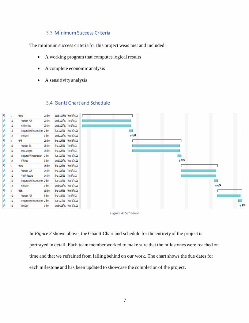
3.4 Gantt Chart and Schedule

In Figure 3 shown above, the Ghantt Chart and schedule for the entirety of the project is

portrayed in detail. Each team member worked to make sure that the milestones were reached on

time and that we refrained from falling behind on our work. The chart shows the due dates for

each milestone and has been updated to showcase the completion of the project.

Figure 4: Schedule

8

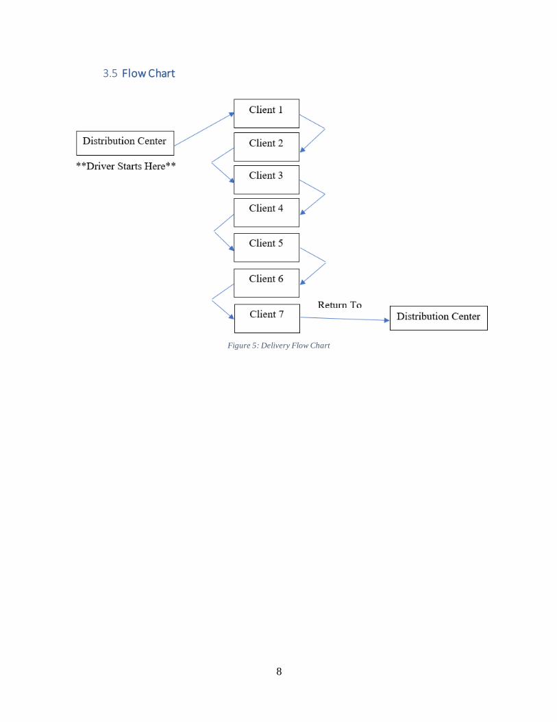
3.5 Flow Chart

Figure 5: Delivery Flow Chart

9

3.6 Responsibilities

Over the course of this project the roles were listed as follows: Adam Esasky is the

Project Manager, and his duties included making sure that the deadlines was met and that we did

not fall behind on the project by having a clear and outlined schedule for the group to follow. He

also assisted in the data programming and software design of the project as well as conducting

the economic analysis for the project. Sean Jones is the Technical Expert, and his duties

involved developing the program in excel and getting it to run correctly while making sure that

the solution to the program gave a logical and correct outcome. He also completed the sensitivity

analysis on our results which helped the company see the alternatives and take action when

variables changed the results. Mark Iltsenko is the Financial Officer, and his duties were to

maintain and keep up with our budget throughout the entirety of the project. Matthew Tharakan

was the Field Expert, and his role was to gather resources from outside industries and use those

to help us gauge what our problem was and how we should look to solve it.

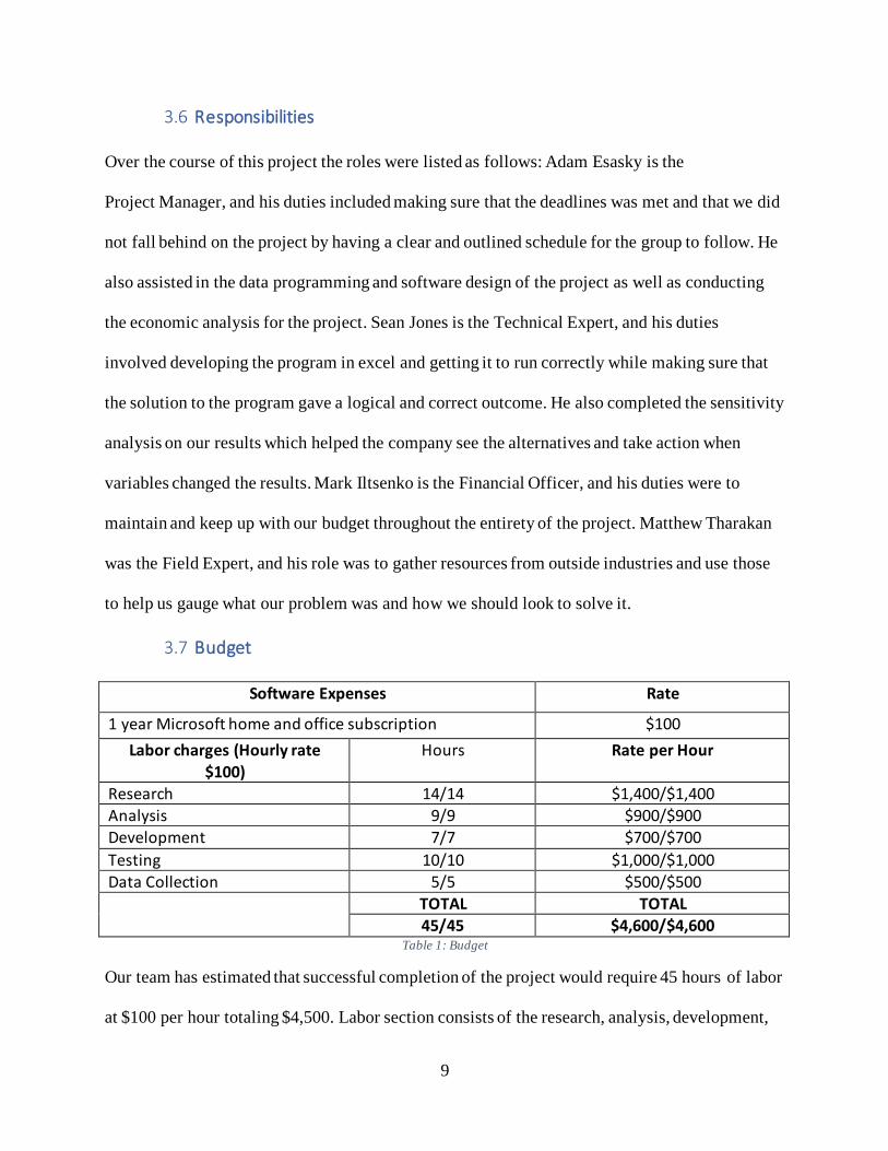
3.7 Budget

Software Expenses Rate

1 year Microsoft home and office subscription $100

Labor charges (Hourly rate $100)

Hours Rate per Hour

Research 14/14 $1,400/$1,400

Analysis 9/9 $900/$900

Development 7/7 $700/$700

Testing 10/10 $1,000/$1,000

Data Collection 5/5 $500/$500

TOTAL TOTAL

45/45 $4,600/$4,600 Table 1: Budget

Our team has estimated that successful completion of the project would require 45 hours of labor

at $100 per hour totaling $4,500. Labor section consists of the research, analysis, development,

10

testing, and data collection. In addition, we have included the Microsoft Office subscription into

software expense which cost $100 online. All these expenses including labor and software made

the project budget to be estimated at $4,600. The amount stated in the Figure 1 above is not the

actual amount that our team or the company spent on the development. This is how much we

would have charged the Carrier Company if we were consulting our expertise to them.

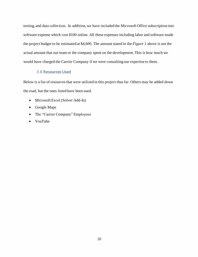
3.8 Resources Used

Below is a list of resources that were utilized in this project thus far. Others may be added down

the road, but the ones listed have been used.

• Microsoft Excel (Solver Add-In)

• Google Maps

• The “Carrier Company” Employees

• YouTube

11

Chapter 4: Solutions

4.1 Proposed Solutions

There are a few kinds of problems regarding the optimal path between locations. Those that we

considered were Dijkstra’s Algorithm, the Traveling Salesman Problem, and the Vehicle Routing

Problem. In the end, we determined that the TSP was how we would be able to solve our

problem. The reasoning why the TSP works best for our problem is because we have multiple

stops in the total trip that need to be optimized. In comparison, the Dijkstra Algorithm is

designed to simply optimize the travel distance between two points. We also chose the TSP

because we only have one delivery driver for the routes whereas the Vehicle Routing Problem is

designed around having multiple vehicles that can complete the delivery instead of just one.

Now that we know that we need to solve a TSP, we need to define multiple things.

4.2 Problem Definition

Our objective function is to minimize the time spent during deliveries. Our variables are the

number of stops and the order of deliveries (8 delivery stops). Our constraints are that the

deliveries must start and end at the distribution center, each stop needs to be visited once, and

there is one driver.

4.3 Solution Methods

Once the problem was defined, the method in which to solve it needed to be determined. Three

different ways were considered: solving by hand, writing a Python program to solve the problem,

and solving in Microsoft Excel. The first method that we eliminated was solving the problem by

hand. The next method we eliminated was creating a Python code to solve the problem. Initial

work on this method was completed but the team’s lack of experience in this field eventually

made us stop working on it. That left solving the problem in Excel.

12

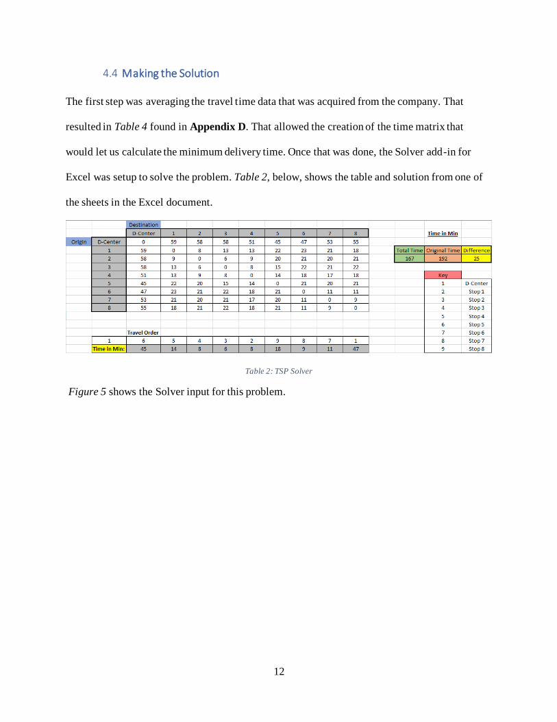
4.4 Making the Solution

The first step was averaging the travel time data that was acquired from the company. That

resulted in Table 4 found in Appendix D. That allowed the creation of the time matrix that

would let us calculate the minimum delivery time. Once that was done, the Solver add-in for

Excel was setup to solve the problem. Table 2, below, shows the table and solution from one of

the sheets in the Excel document.

Table 2: TSP Solver

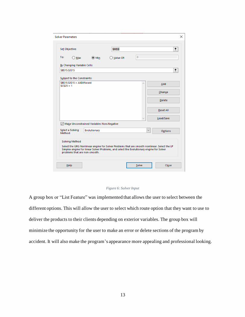
Figure 5 shows the Solver input for this problem.

13

Figure 6: Solver Input

A group box or “List Feature” was implemented that allows the user to select between the

different options. This will allow the user to select which route option that they want to use to

deliver the products to their clients depending on exterior variables. The group box will

minimize the opportunity for the user to make an error or delete sections of the program by

accident. It will also make the program’s appearance more appealing and professional looking.

14

Chapter 5: Analysis

5.1 Verification Approach

In order to confirm whether the new program is a more viable solution for a faster route, a

comparison analysis was done to show the differences between the times of the old route model

and the new route model. An economic analysis will also be used in the next report to help verify

the price saving differences between the two delivery route styles. If the results show shorter

distances traveled, shorter delivery times, and lower expenditure costs then the new route

program will be a more viable and efficient route to take than that of the previous models.

5.2 Time

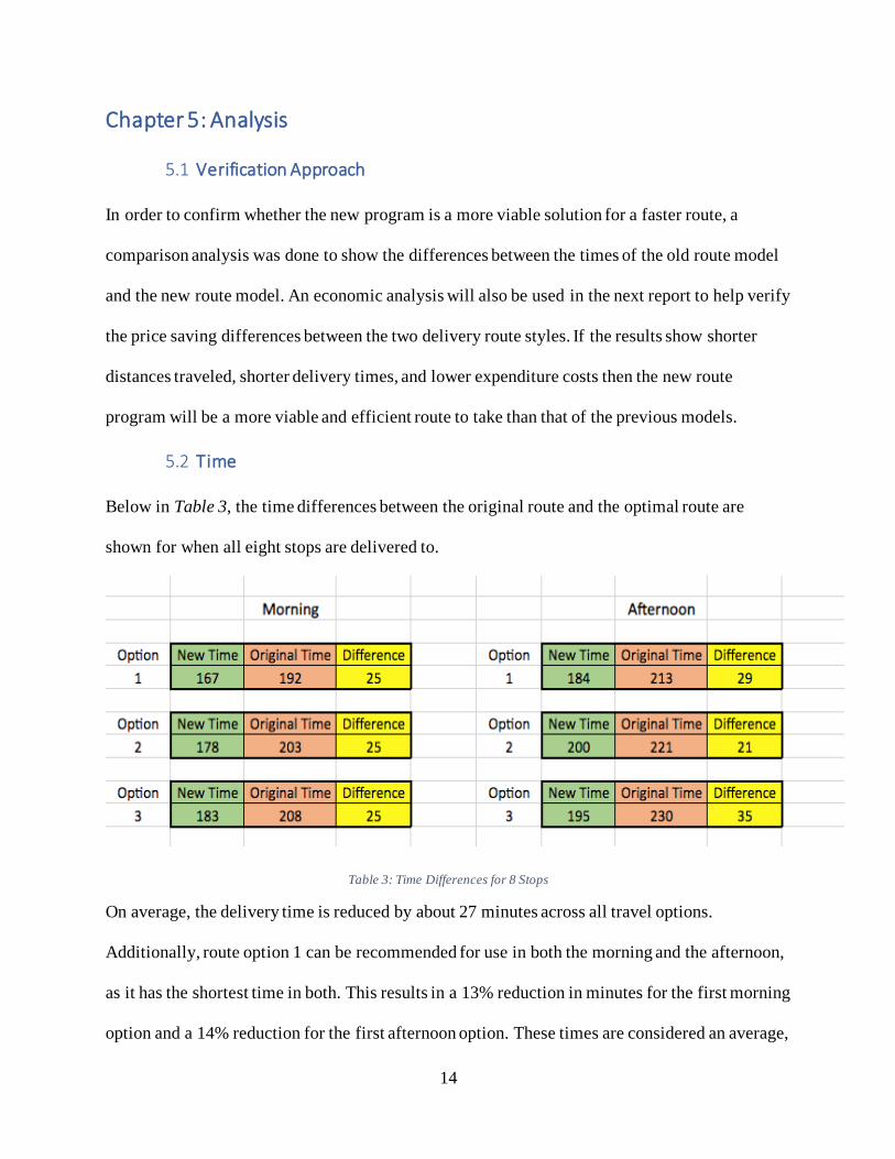
Below in Table 3, the time differences between the original route and the optimal route are

shown for when all eight stops are delivered to.

Table 3: Time Differences for 8 Stops

On average, the delivery time is reduced by about 27 minutes across all travel options.

Additionally, route option 1 can be recommended for use in both the morning and the afternoon,

as it has the shortest time in both. This results in a 13% reduction in minutes for the first morning

option and a 14% reduction for the first afternoon option. These times are considered an average,

15

and sources of uncertainty include unexpected traffic on-route and lunch stops for the drivers

depending on the time of day they start their route from the Carrier’s location.

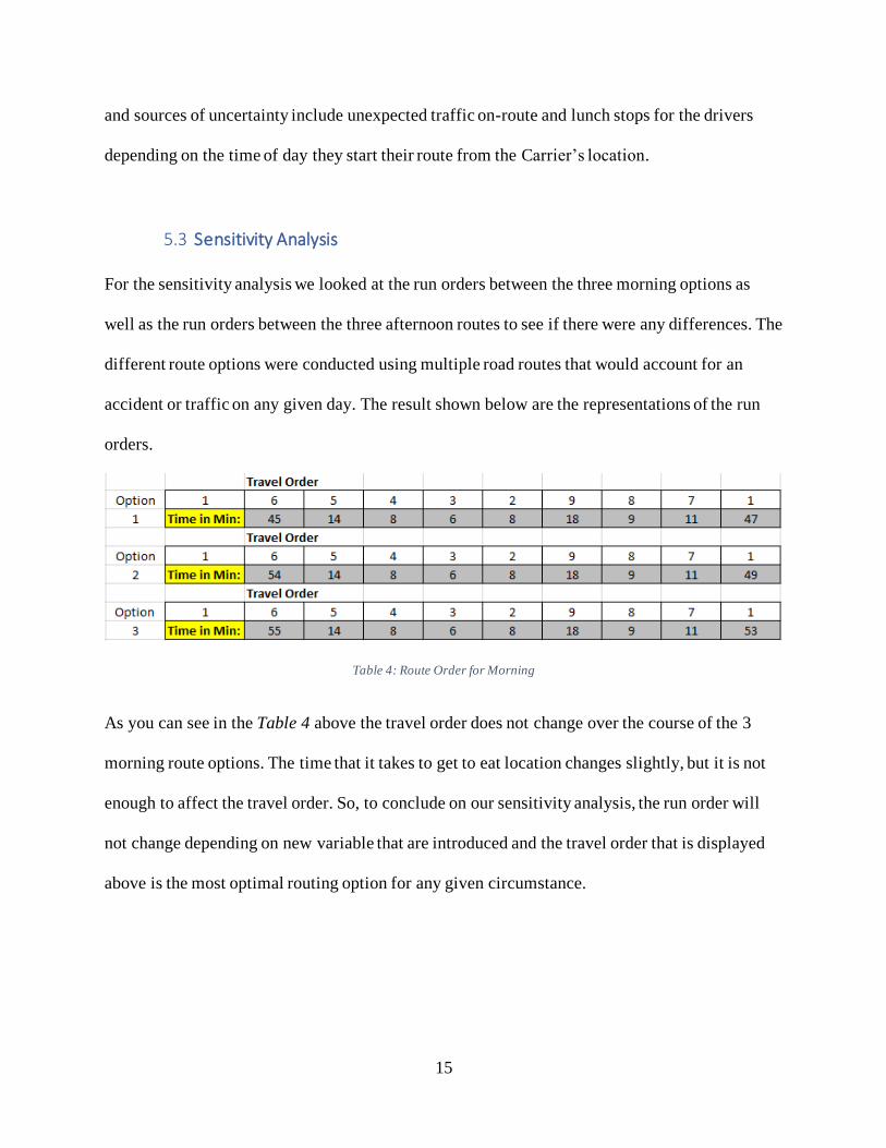
5.3 Sensitivity Analysis

For the sensitivity analysis we looked at the run orders between the three morning options as

well as the run orders between the three afternoon routes to see if there were any differences. The

different route options were conducted using multiple road routes that would account for an

accident or traffic on any given day. The result shown below are the representations of the run

orders.

Table 4: Route Order for Morning

As you can see in the Table 4 above the travel order does not change over the course of the 3

morning route options. The time that it takes to get to eat location changes slightly, but it is not

enough to affect the travel order. So, to conclude on our sensitivity analysis, the run order will

not change depending on new variable that are introduced and the travel order that is displayed

above is the most optimal routing option for any given circumstance.

16

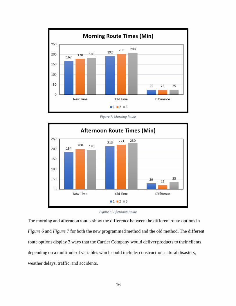
The morning and afternoon routes show the difference between the different route options in

Figure 6 and Figure 7 for both the new programmed method and the old method. The different

route options display 3 ways that the Carrier Company would deliver products to their clients

depending on a multitude of variables which could include: construction, natural disasters,

weather delays, traffic, and accidents.

Figure 7: Morning Route

Figure 8: Afternoon Route

17

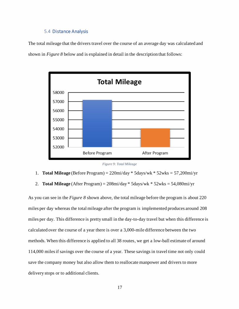
5.4 Distance Analysis

The total mileage that the drivers travel over the course of an average day was calculated and

shown in Figure 8 below and is explained in detail in the description that follows:

1. Total Mileage (Before Program) = 220mi/day * 5days/wk * 52wks = 57,200mi/yr

2. Total Mileage (After Program) = 208mi/day * 5days/wk * 52wks = 54,080mi/yr

As you can see in the Figure 8 shown above, the total mileage before the program is about 220

miles per day whereas the total mileage after the program is implemented produces around 208

miles per day. This difference is pretty small in the day-to-day travel but when this difference is

calculated over the course of a year there is over a 3,000-mile difference between the two

methods. When this difference is applied to all 38 routes, we get a low-ball estimate of around

114,000 miles if savings over the course of a year. These savings in travel time not only could

save the company money but also allow them to reallocate manpower and drivers to more

delivery stops or to additional clients.

Figure 9: Total Mileage

18

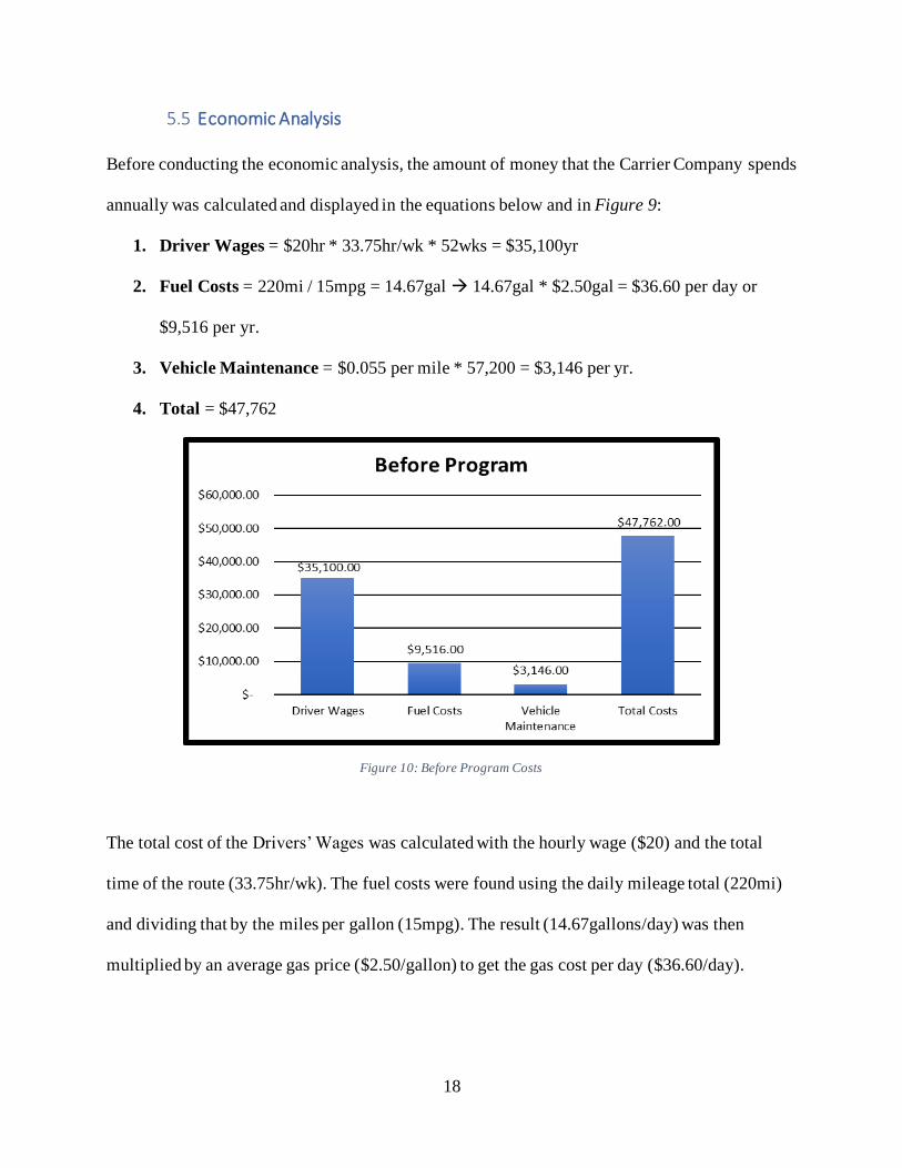
5.5 Economic Analysis

Before conducting the economic analysis, the amount of money that the Carrier Company spends

annually was calculated and displayed in the equations below and in Figure 9:

1. Driver Wages = $20hr * 33.75hr/wk * 52wks = $35,100yr

2. Fuel Costs = 220mi / 15mpg = 14.67gal → 14.67gal * $2.50gal = $36.60 per day or

$9,516 per yr.

3. Vehicle Maintenance = $0.055 per mile * 57,200 = $3,146 per yr.

4. Total = $47,762

The total cost of the Drivers’ Wages was calculated with the hourly wage ($20) and the total

time of the route (33.75hr/wk). The fuel costs were found using the daily mileage total (220mi)

and dividing that by the miles per gallon (15mpg). The result (14.67gallons/day) was then

multiplied by an average gas price ($2.50/gallon) to get the gas cost per day ($36.60/day).

Figure 10: Before Program Costs

19

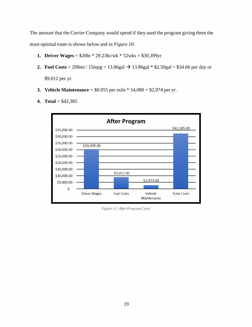
The amount that the Carrier Company would spend if they used the program giving them the

most optimal route is shown below and in Figure 10:

1. Driver Wages = $20hr * 29.23hr/wk * 52wks = $30,399yr

2. Fuel Costs = 208mi / 15mpg = 13.86gal → 13.86gal * $2.50gal = $34.66 per day or

$9,012 per yr.

3. Vehicle Maintenance = $0.055 per mile * 54,080 = $2,974 per yr.

4. Total = $42,385

Figure 11: After Program Costs

20

For the programmed route, the driver wages were calculated by using the company’s rate per

hour of a delivery drivers ($20hr). The fuel costs were determined by taking the daily total of

mileage (208mi) and dividing that by the average miles per gallon (15mpg) that the company

vehicles get (13.86gal). The next step was to take the total gallons used and multiply that by the

average gas price per gallon ($2.50) to get the daily total fuel cost of the route ($34.66).

As you can see in in Figure 11 shown above, the company costs collectively were lower after

using the optimized route as opposed to when the company ran operations before the route was

optimized. The valued differences between the fuel costs and vehicle maintenance were not that

drastic in the small scale of total savings but if you were to take those differences and compute

them over the 38 other routes, then the costs difference would be significant enough to make the

program a viable cost saving option ($25,688).

Figure 12: Company Costs

21

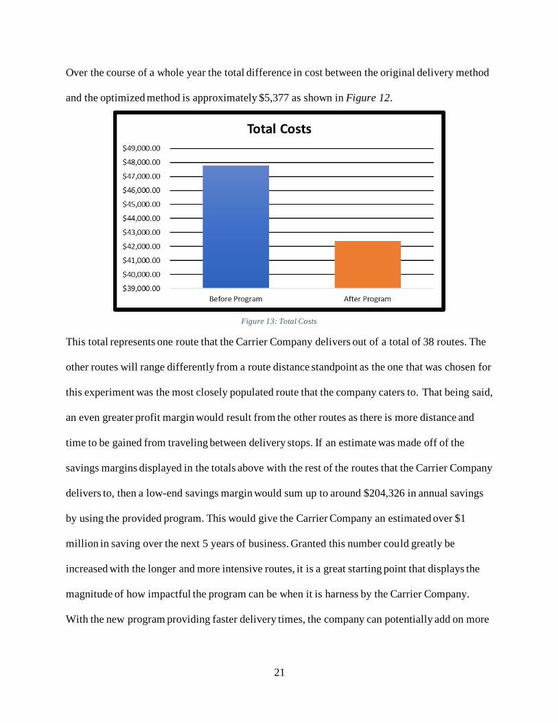
Over the course of a whole year the total difference in cost between the original delivery method

and the optimized method is approximately $5,377 as shown in Figure 12.

This total represents one route that the Carrier Company delivers out of a total of 38 routes. The

other routes will range differently from a route distance standpoint as the one that was chosen for

this experiment was the most closely populated route that the company caters to. That being said,

an even greater profit margin would result from the other routes as there is more distance and

time to be gained from traveling between delivery stops. If an estimate was made off of the

savings margins displayed in the totals above with the rest of the routes that the Carrier Company

delivers to, then a low-end savings margin would sum up to around $204,326 in annual savings

by using the provided program. This would give the Carrier Company an estimated over $1

million in saving over the next 5 years of business. Granted this number could greatly be

increased with the longer and more intensive routes, it is a great starting point that displays the

magnitude of how impactful the program can be when it is harness by the Carrier Company.

With the new program providing faster delivery times, the company can potentially add on more

Figure 13: Total Costs

22

clients and stops to each route which would allow them to make even more money by increasing

the total number of products delivered on each route.

23

Chapter 6: Results and Discussion

6.1 Summary of Analysis

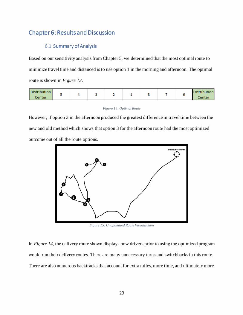
Based on our sensitivity analysis from Chapter 5, we determined that the most optimal route to

minimize travel time and distanced is to use option 1 in the morning and afternoon. The optimal

route is shown in Figure 13.

Figure 14: Optimal Route

However, if option 3 in the afternoon produced the greatest difference in travel time between the

new and old method which shows that option 3 for the afternoon route had the most optimized

outcome out of all the route options.

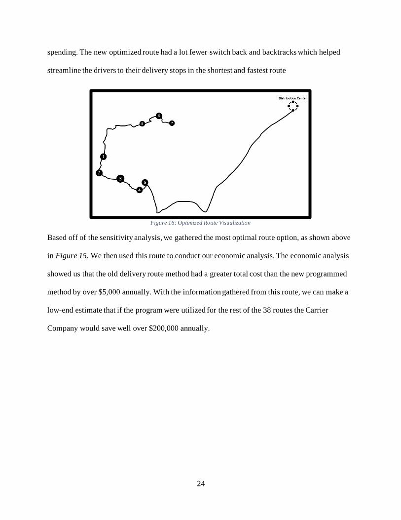
In Figure 14, the delivery route shown displays how drivers prior to using the optimized program

would run their delivery routes. There are many unnecessary turns and switchbacks in this route.

There are also numerous backtracks that account for extra miles, more time, and ultimately more

Figure 15: Unoptimized Route Visualization

24

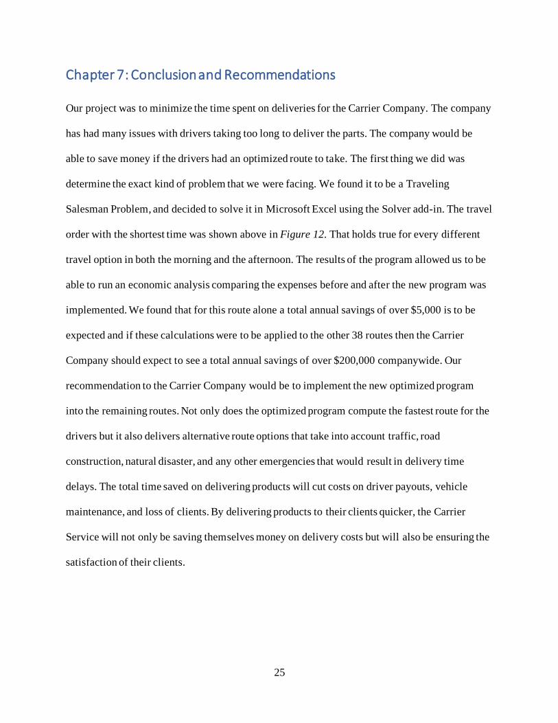
spending. The new optimized route had a lot fewer switch back and backtracks which helped

streamline the drivers to their delivery stops in the shortest and fastest route

Based off of the sensitivity analysis, we gathered the most optimal route option, as shown above

in Figure 15. We then used this route to conduct our economic analysis. The economic analysis

showed us that the old delivery route method had a greater total cost than the new programmed

method by over $5,000 annually. With the information gathered from this route, we can make a

low-end estimate that if the program were utilized for the rest of the 38 routes the Carrier

Company would save well over $200,000 annually.

Figure 16: Optimized Route Visualization

25

Chapter 7: Conclusion and Recommendations

Our project was to minimize the time spent on deliveries for the Carrier Company. The company

has had many issues with drivers taking too long to deliver the parts. The company would be

able to save money if the drivers had an optimized route to take. The first thing we did was

determine the exact kind of problem that we were facing. We found it to be a Traveling

Salesman Problem, and decided to solve it in Microsoft Excel using the Solver add-in. The travel

order with the shortest time was shown above in Figure 12. That holds true for every different

travel option in both the morning and the afternoon. The results of the program allowed us to be

able to run an economic analysis comparing the expenses before and after the new program was

implemented. We found that for this route alone a total annual savings of over $5,000 is to be

expected and if these calculations were to be applied to the other 38 routes then the Carrier

Company should expect to see a total annual savings of over $200,000 companywide. Our

recommendation to the Carrier Company would be to implement the new optimized program

into the remaining routes. Not only does the optimized program compute the fastest route for the

drivers but it also delivers alternative route options that take into account traffic, road

construction, natural disaster, and any other emergencies that would result in delivery time

delays. The total time saved on delivering products will cut costs on driver payouts, vehicle

maintenance, and loss of clients. By delivering products to their clients quicker, the Carrier

Service will not only be saving themselves money on delivery costs but will also be ensuring the

satisfaction of their clients.

26

References

▪ Dantzig, George B., and John H. Ramser. "The truck dispatching problem." Management

science 6.1 (1959): 80-91.

▪ Tyagi, M. "A practical method for the truck dispatching problem." Journal of the

Operations Research Society of Japan 10 (1968): 76-92.

▪ Rego, César, and Catherine Roucairol. "Using tabu search for solving a dynamic multi -

terminal truck dispatching problem." European Journal of Operational Research 83.2

(1995): 411-429.

▪ Duan, C. J., et al. “Using Excel Solver to Solve Braydon Farms’ Truck Routing Problem:

A Case Study.” South Asian Journal of Management Sciences, vol. 10, no. 1, Spring

2016, pp. 38–47. EBSCOhost, doi:10.21621/sajms.2016101.04.

▪ RANÇA PAULO M., et al. “The M-Traveling Salesman Problem with Minmax

Objective.” Transportation Science, vol. 29, no. 3, Aug. 1995, pp. 267–275. EBSCOhost,

search.ebscohost.com/login.aspx?direct=true&AuthType=ip,shib&db=edsjsr&AN=edsjsr

.25768693&site=eds-live&scope=site.

▪ Rego, Cesar, and Catherine Roucairol. “Using Tabu Search for Solving a Dynamic Multi-

Terminal Truck Dispatching Problem.” European Journal of Operational Research, vol.

83, no. 2, June 1995, p. 411. EBSCOhost,

search.ebscohost.com/login.aspx?direct=true&AuthType=ip,shib&db=edsggo&AN=edsg

cl.16963339&site=eds-live&scope=site.

▪ Bixby, R. E. (. 1. )., and E. K. (. 2. ). Lee. “Solving a Truck Dispatching Scheduling

Problem Using Branch-and-Cut.” Operations Research, vol. 46, no. 3, pp. 355–367.

EBSCOhost, doi:10.1287/opre.46.3.355. Accessed 23 Mar. 2021.

27

▪ Alhassan Sulemana, et al. “Effect of Optimal Routing on Travel Distance, Travel Time

and Fuel Consumption of Waste Collection Trucks.” Management of Environmental

Quality: An International Journal, vol. 30, no. 4, June 2019, pp. 803–832. EBSCOhost,

doi:10.1108/MEQ-07-2018-0134.

▪ Gendereau, Michel, and Christos Tarantilis. “Solving Large-Scale Vehicle Routing

Problems with Time Windows: The State-of-the-Art.” Interuniversity Research Center,

2010, www.cirrelt.ca/documentstravail/cirrelt-2010-04.pdf.

▪ Choi, H. R., et al. “Dispatching of Container Trucks Using Genetic Algorithm.” The 4th

International Conference on Interaction Sciences, Interaction Sciences (ICIS), 2011 4th

International Conference On, Aug. 2011, pp. 146–151. EBSCOhost,

search.ebscohost.com/login.aspx?direct=true&AuthType=ip,shib&db=edseee&AN=edse

ee.6014548&site=eds-live&scope=site.

▪ Srour, F.Jordan, et al. “Strategies for Handling Temporal Uncertainty in Pickup and

Delivery Problems with Time Windows.” Transportation Science, vol. 52, no. 1, Jan.

2018, pp. 3–19. EBSCOhost, doi:10.1287/trsc.2015.0658.

▪ Schneider, Michael, et al. “The Electric Vehicle-Routing Problem with Time Windows

and Recharging Stations.” Transportation Science, vol. 48, no. 4, Nov. 2014, p. 500.

EBSCOhost, doi:10.1287/trsc.2013.0490.

▪ ResearchGate, www.researchgate.net/figure/Illustration-of-the-traveling-salesman-

problem-TSP-and-vehicle-route-problem-VRP_fig1_277673931.

▪ Semantic Scholar, 2013, www.semanticscholar.org/paper/Memetic-Algorithm-for-a-

Multi-Objective-Vehicle-Ayadi

Benadada/6d1887403b13935ed83d650beb350ddca0c9eb60.

28

Appendix A: Acknowledgements

Team Drive Fast would like to thank the Carrier Company for allowing us the chances to help

work on and develop a program that not only improves the delivery time and speed but also cuts

down on total costs of running the business. Special thanks to the Project Manager for helping us

gather key information on the previous delivery method as well as the current expenditures that

the company spends each year prior to having the program running. We would also like to thank

the delivery drivers for helping us gather accurate delivery times before the program was run as

well as after the program was incorporated.

29

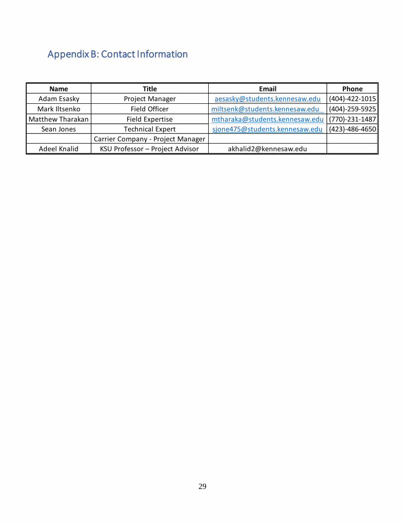
Appendix B: Contact Information

Name Title Email Phone

Adam Esasky Project Manager aesasky@students.kennesaw.edu (404)-422-1015

Mark Iltsenko Field Officer miltsenk@students.kennesaw.edu (404)-259-5925

Matthew Tharakan Field Expertise mtharaka@students.kennesaw.edu (770)-231-1487

Sean Jones Technical Expert sjone475@students.kennesaw.edu (423)-486-4650

Carrier Company - Project Manager

Adeel Knalid KSU Professor – Project Advisor akhalid2@kennesaw.edu

30

Appendix C: Reflections

Adam Esasky – This project taught me a lot about the transportation industry and the lengths

that one has to go in order to develop a program that optimizes a delivery route. If I was to do a

similar type of project in the future I would probably teach myself to code so that I could

program the solution in either Python or MATLAB. I enjoyed being able to see the real-world

applications of the lessons that I had learned over the years in college. This project helped paint a

picture of how Industrial Engineering is used and conducted in the business world as well as

areas where Industrial Engineering still needs to be introduced. I would also like to thank the

employees over at the Carrier Company for their patience and willingness to help us solve the

problem and work with us on getting the program implemented into their delivery services.

Mark Iltsenko – I enjoyed working on the project like this. Throughout this project I was able to

apply a lot of concepts that I learned in other ISYE courses. This senior design project gave me

an opportunity to understand better how projects are developed and implemented. This work

gave me greater insight of what Industrial Engineers do in the real world. This project is another

example of how software can improve the complicated world of supply chain and in particular

the logistics aspect of it. There is a lot of inefficiencies in the world of logistics that can be

reduced with simple and affordable software like excel with minimum investments. Overall, I am

glad that I had the opportunity to work on this project. Now I understand how IEs bring value to

businesses by optimizing their processes.

Matthew Tharakan –

Working on this opened my eyes

Applies to real-world applications

31

Sean Jones – Overall, I enjoyed working on this project. I came into this project with some very

high hopes and expectations on what we would be able to achieve. I had ideas of creating a

professional-quality program that anyone could have used. However, it quickly became apparent

that none of us had the technical knowledge to code such a program. I learned then that you need

to take stock of your team’s capabilities when starting a project. This project has made me

consider the possibility of consulting in the future.

32

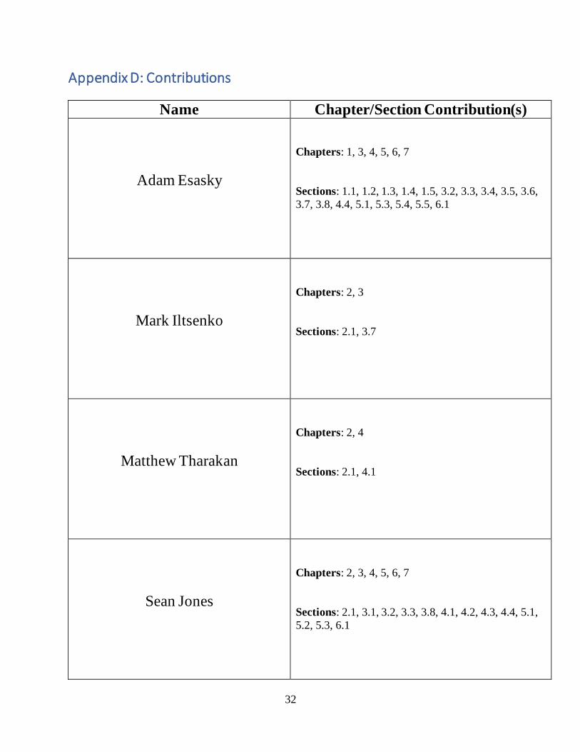
Appendix D: Contributions

Name Chapter/Section Contribution(s)

Adam Esasky

Chapters: 1, 3, 4, 5, 6, 7

Sections: 1.1, 1.2, 1.3, 1.4, 1.5, 3.2, 3.3, 3.4, 3.5, 3.6,

3.7, 3.8, 4.4, 5.1, 5.3, 5.4, 5.5, 6.1

Mark Iltsenko

Chapters: 2, 3

Sections: 2.1, 3.7

Matthew Tharakan

Chapters: 2, 4

Sections: 2.1, 4.1

Sean Jones

Chapters: 2, 3, 4, 5, 6, 7

Sections: 2.1, 3.1, 3.2, 3.3, 3.8, 4.1, 4.2, 4.3, 4.4, 5.1,

5.2, 5.3, 6.1

33

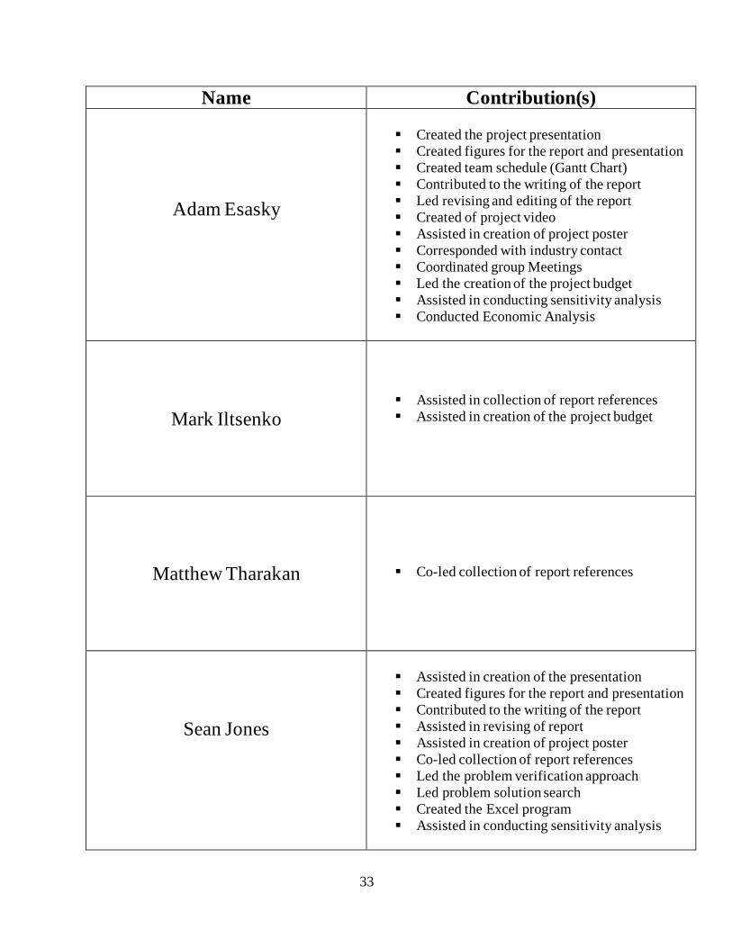
Name Contribution(s)

Adam Esasky

▪ Created the project presentation

▪ Created figures for the report and presentation

▪ Created team schedule (Gantt Chart)

▪ Contributed to the writing of the report

▪ Led revising and editing of the report

▪ Created of project video

▪ Assisted in creation of project poster

▪ Corresponded with industry contact

▪ Coordinated group Meetings

▪ Led the creation of the project budget

▪ Assisted in conducting sensitivity analysis

▪ Conducted Economic Analysis

Mark Iltsenko

▪ Assisted in collection of report references

▪ Assisted in creation of the project budget

Matthew Tharakan

▪ Co-led collection of report references

Sean Jones

▪ Assisted in creation of the presentation

▪ Created figures for the report and presentation

▪ Contributed to the writing of the report

▪ Assisted in revising of report

▪ Assisted in creation of project poster

▪ Co-led collection of report references

▪ Led the problem verification approach

▪ Led problem solution search

▪ Created the Excel program

▪ Assisted in conducting sensitivity analysis

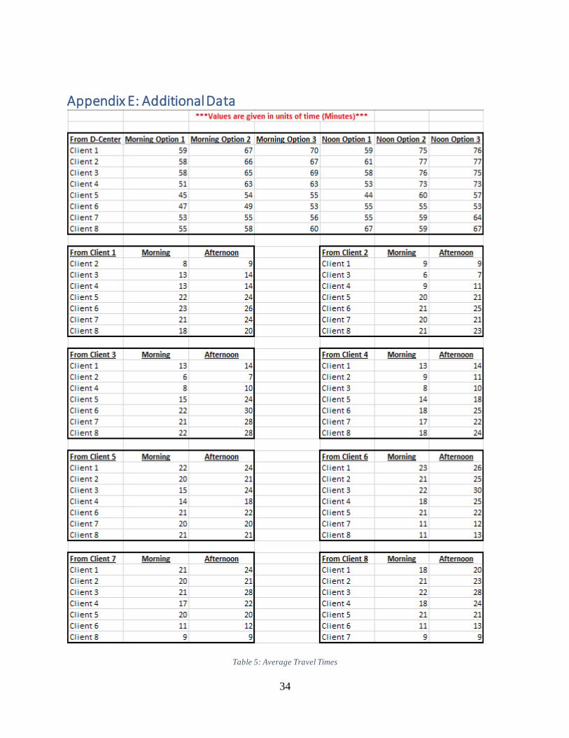
34

Appendix E: Additional Data

Table 5: Average Travel Times