delivery truck assignment for supply chain management
TRANSCRIPT

Delivery Truck Assignment for Supply Chain Management
Tiago Simoes Costa
Thesis to obtain the Master of Science Degree in
Mechanical Engineering
Supervisors: Prof. Joao Miguel da Costa SousaEng. Miguel de Sousa Esteves Martins
Examination Committee
Chairperson: Prof. Name of the ChairpersonSupervisor: Prof. Joao Miguel da Costa Sousa
Members of the Committee: Prof. Name of First Committee MemberDr. Name of Second Committee MemberEng. Name of Third Committee Member
October 2020


Acknowledgments
I would like to thank my supervisors Prof. Joao Sousa and Eng. Miguel Martins for the support and
their insights that made his thesis possible. I would also like to thank Prof. Susana Vieira and Joaquim
Viegas, PhD. I would also like to thank all the Business Intelligence team in Worten in Diana, Hugo, Ines,
Margarida, Miguel, Pedro and Rita for all the support and business insights.
Last but not least, to my family, my friends and colleagues that helped throughout this years. Thank
you.
To each and every one of you – Thank you.


Abstract
Now, more than ever, the efficiency in transportation of goods is of extreme importance. According
to the European Environment Agency, in average only 70% of the available truck capacity is used.
Inefficient product delivery is not only a waste of money but it also negatively impacts the environment.
Thus, it is pivotal to develop efficient and cost-effective solutions for the delivery of goods. This thesis
studies a supply chain management problem where the goal is to minimize the global cost of the supply
chain operation. The presented approach takes into account due dates and effectively increases the
efficiency of truck capacity. The approach consist of using an optimization method to find the best
assignment assignment of weekly orders to trucks not only by their routes, but also by their delivery
day. For this optimization problem it was used a Local Search Algorithm, a Genetic Algorithm and also
a hybrid approach between these two. It was possible to observe good results from all of the algorithms
when applied to a real case study and compared with the solution currently deployed, specially the
hybrid of the Genetic Algorithm and Local Search Algorithm.
Keywords
Vehicles Routing Problem, Assignment Problem, Genetic Algorithm, Local Search, Supply Chain Man-
agement
iii


Resumo
Agora, mais do que nunca, a eficiencia no transporte de mercadorias e de extrema importancia. De
acordo com a Agencia Europeia do Ambiente, em media, apenas 70 % da capacidade disponıvel do
camiao e utilizada. A entrega ineficiente de produtos nao e apenas um desperdıcio de dinheiro, mas
tambem causa um impacto negativo no meio ambiente. Portanto, e fundamental desenvolver solucoes
eficientes e economicas para a entrega de mercadorias. Esta tese estuda um problema de gestao da
cadeia de abastecimento onde o objetivo e minimizar o custo global da operacao de supply chain. A
abordagem apresentada tem em consideracao as datas limite de entrega e aumenta a eficiencia da ca-
pacidade dos camioes. Esta tecnica sera um metodo de otimizacao para a atribuicao de encomendas
semanais aos camioes nao so pelos percursos, mas tambem pelo dia de entrega. Para esta tecnica
de otimizacao foi utilizado um Algoritmo de Pesquisa Local, um Algoritmo Genetico e tambem uma
abordagem hıbrida entre os dois. Foi possıvel observar bons resultados de todos os algoritmos quando
aplicados a um estudo de caso real e comparados com a solucao atualmente implementada, principal-
mente o hıbrido de Algoritmo Genetico e Algoritmo de Pesquisa Local.
Palavras Chave
Problema de Roteamento de Veıculos, Problema de Atribuicao, Algoritmo Genetico, Pesquisa Local,
Gestao da Cadeia de Abastecimento
v


Contents
1 Introduction 1
1.1 Motivation . . . . . . . . . . . . . . . . . . . . . . . . . . . . . . . . . . . . . . . . . . . . . 1
1.2 Objectives . . . . . . . . . . . . . . . . . . . . . . . . . . . . . . . . . . . . . . . . . . . . . 3
1.3 Contributions . . . . . . . . . . . . . . . . . . . . . . . . . . . . . . . . . . . . . . . . . . . 3
1.4 Thesis Outline . . . . . . . . . . . . . . . . . . . . . . . . . . . . . . . . . . . . . . . . . . 4
2 Supply Chain Management in Distribution Optimization 5
2.1 Approaches to SCM . . . . . . . . . . . . . . . . . . . . . . . . . . . . . . . . . . . . . . . 5
2.1.1 Warehouse Optimization . . . . . . . . . . . . . . . . . . . . . . . . . . . . . . . . 6
2.1.2 Transportation Optimization . . . . . . . . . . . . . . . . . . . . . . . . . . . . . . . 7
2.2 Methods to solve a SCM optimization problem . . . . . . . . . . . . . . . . . . . . . . . . 9
2.2.1 Auto Regressive Integrated Moving Average . . . . . . . . . . . . . . . . . . . . . . 9
2.2.2 Hill Climbing . . . . . . . . . . . . . . . . . . . . . . . . . . . . . . . . . . . . . . . 9
2.2.3 Ant colony optimization . . . . . . . . . . . . . . . . . . . . . . . . . . . . . . . . . 10
2.2.4 Genetic Algorithm . . . . . . . . . . . . . . . . . . . . . . . . . . . . . . . . . . . . 11
2.2.5 Exact Algorithms . . . . . . . . . . . . . . . . . . . . . . . . . . . . . . . . . . . . . 14
3 Delivery Truck Assignment 15
3.1 Current Transportation Model . . . . . . . . . . . . . . . . . . . . . . . . . . . . . . . . . . 15
3.2 Problem Approach . . . . . . . . . . . . . . . . . . . . . . . . . . . . . . . . . . . . . . . . 17
3.3 Mathematical Formulation . . . . . . . . . . . . . . . . . . . . . . . . . . . . . . . . . . . . 18
4 Proposed Methods 23
4.1 Initial Solution . . . . . . . . . . . . . . . . . . . . . . . . . . . . . . . . . . . . . . . . . . . 23
4.2 Evaluation . . . . . . . . . . . . . . . . . . . . . . . . . . . . . . . . . . . . . . . . . . . . . 24
4.2.1 Capacitated Vehicle Routing Problem . . . . . . . . . . . . . . . . . . . . . . . . . 25
4.3 Genetic Algorithm . . . . . . . . . . . . . . . . . . . . . . . . . . . . . . . . . . . . . . . . 26
4.4 Local Search Algorithm . . . . . . . . . . . . . . . . . . . . . . . . . . . . . . . . . . . . . 30
4.5 Exact Algorithm . . . . . . . . . . . . . . . . . . . . . . . . . . . . . . . . . . . . . . . . . . 30
4.6 Hybrid Algorithm . . . . . . . . . . . . . . . . . . . . . . . . . . . . . . . . . . . . . . . . . 31
vii

4.7 Brief software explanation . . . . . . . . . . . . . . . . . . . . . . . . . . . . . . . . . . . . 31
5 Results and Discussion 33
5.1 Demand data . . . . . . . . . . . . . . . . . . . . . . . . . . . . . . . . . . . . . . . . . . . 33
5.2 Data analysis . . . . . . . . . . . . . . . . . . . . . . . . . . . . . . . . . . . . . . . . . . . 34
5.3 Parameter Configuration . . . . . . . . . . . . . . . . . . . . . . . . . . . . . . . . . . . . . 35
5.3.1 Population size and number of offsprings . . . . . . . . . . . . . . . . . . . . . . . 35
5.3.2 Number of crossover points . . . . . . . . . . . . . . . . . . . . . . . . . . . . . . . 36
5.3.3 Number of generations . . . . . . . . . . . . . . . . . . . . . . . . . . . . . . . . . 36
5.4 Results . . . . . . . . . . . . . . . . . . . . . . . . . . . . . . . . . . . . . . . . . . . . . . 36
5.4.1 Local Search Algorithm . . . . . . . . . . . . . . . . . . . . . . . . . . . . . . . . . 37
5.4.2 Genetic Algorithm . . . . . . . . . . . . . . . . . . . . . . . . . . . . . . . . . . . . 38
5.4.3 Hybrid Algorithm . . . . . . . . . . . . . . . . . . . . . . . . . . . . . . . . . . . . . 39
5.5 Discussion . . . . . . . . . . . . . . . . . . . . . . . . . . . . . . . . . . . . . . . . . . . . 41
5.5.1 Final Results . . . . . . . . . . . . . . . . . . . . . . . . . . . . . . . . . . . . . . . 41
5.5.2 In-Evaluation vs Out-Evaluation . . . . . . . . . . . . . . . . . . . . . . . . . . . . . 41
5.5.3 LSA vs GA vs Hybrid . . . . . . . . . . . . . . . . . . . . . . . . . . . . . . . . . . 42
6 Conclusions 43
6.1 Future Work . . . . . . . . . . . . . . . . . . . . . . . . . . . . . . . . . . . . . . . . . . . . 44
List of Tables . . . . . . . . . . . . . . . . . . . . . . . . . . . . . . . . . . . . . . . . . . . . . . 45
List of Figures . . . . . . . . . . . . . . . . . . . . . . . . . . . . . . . . . . . . . . . . . . . . . 47
viii

1Introduction
1.1 Motivation
With emerging challenges everyday the biggest retail companies need to keep up with the technology
innovation otherwise they will lose to their direct competition. In this sense retail companies spend
more and more resources trying to figure out ways to improve their operations. As discussed in [1], the
major challenges retail companies face are the growth of e-commerce, customer loyalty, service success
strategies and the behavioral issues in pricing and patronage. Out of these four topics only behavioral
issues in pricing and patronage is not affected by the supply chain. With the growth of e-commerce,
the delivery dynamics changes and the supply chain operation has to adjust. E-commerce created a
sense of power to the customer where he decides when and where he wants to receive products in short
periods of time, increasing the uncertainty. The supplier adjusts to this complexity by having dynamic
routes that change during the year based on the forecasted demand.
The quality of service when it comes to delivering it to a customer when requested highly influences
the customer loyalty. If a company can deliver the same product with twice the speed as its competitor
this will be a factor taken into account by the customer when choosing where to buy. How a customer
1

is served is an important factor in customer loyalty, and most changes in demand imply challenges in
the supply chain operation. One example of this is a company A that offers a service with same day
delivery, where a customer buys an appliance online and receives it in the same day. The customer will
have more loyalty towards it than a company B that can only deliver a week later. Competitive delivery
times are a driving factor for customer loyalty, but imply big challenges in the distribution of products and
in the organization of warehouse. It is important to find a balance between serving the customers well
and not compromising resources in this highly dynamic operation.
The motivation for this work detailed in this thesis came from a real world company, Worten, and
their need to adapt to these new challenges. With the growth of e-commerce it is imperative to have
an effective supply chain that grants low costs in the total operation without compromising customer
satisfaction. Also with the increasing fuel costs and the growing concern with greenhouse gas emissions
at a global level there is an urge in reducing the number of circulating trucks.
Worten’s business in Portugal and Spain is very distinct due to geographical differences and different
densities in the number of stores. The bigger size of Spain and the lower density of stores creates a
bigger distance between stores and the customers, as shown in Figure 1.1. This is why the problem
previously referred is much more challenging in Spain and the reason the focus of this project will be in
this country.
Figure 1.1: Comparison the number of stores in Portugal and in Spain
2

1.2 Objectives
The main goal of this thesis is to develop a model that optimizes the weekly assignment of pallets to
trucks based on the store’s demand. This optimization of the supply chain will focus on minimizing
the global costs of the process. This work also tries a different approach to traditional supply chain
optimization models because its main focus is not only to assign pallets to routes but also assign them
to days of the week. This optimization will look at the date a product needs to be delivered and choose
the best day for its delivery while also giving the best routes for each scenario. This model has been
built in a way that is able to handle the yearly demand dynamics shown in Figure 1.2.
Figure 1.2: Normalized typical demand curve during a year in weeks
1.3 Contributions
This work proposes a new approach to delivery assignment in supply chain operations. This includes
three algorithms to approach the optimization of when the pallets should be delivered whitin a week,
point 1,Schedule Pallet Deliveries, and a complementary algorithm that solves the routing of the same
pallets each day, point 2, An exact algorithm to solve a Capacitated Vehicle Routing Problem:
1. Schedule Pallet Deliveries
(a) Local Search Algorithm
(b) Multi-Point Crossover Genetic Algorithm
(c) Hybrid Algorithm combined the Local Search Algorithm and the Multi-Point Crossover Genetic
Algorithm. In this hybrid Algorithm, the Multi-Point Crossover Genetic Algorithm is used as a
method to create the Local Search’s first solution.
2. An exact algorithm to solve a Capacitated Vehicle Routing Problem
3

1.4 Thesis Outline
This thesis is organized in the following chapters:
• Chapter 1 – Introduction: In the first chapter, a brief presentation about the context of the problem
and about supply chain was given.
• Chapter 2 – Supply Chain Management Optimization: The Supply Chain Management Opti-
mization chapter aims to explore what already exists in literature that is related to the problem at
hand.
• Chapter 3 – Delivery Truck Assignment: In this chapter it is presented how the problem is going
to be formulated, cost functions, restrictions, simplifications. Small use cases are given to explain
it in a more illustrative way.
• Chapter 4 – Proposed Methods: The used algorithms are explained in this chapter, namely:
Local Search, Multi-Point Crossover Genetic Algorithm and a Hybrid Algorithm.
• Chapter 5 – Results and Discussion: The results are presented and discussed in this chapter.
• Chapter 6 – Conclusions: In this final chapter relevant conclusions are presented and sugges-
tions about what can be done as future work to further develop this topic.
4

2Supply Chain Management in
Distribution Optimization
Supply Chain Management (SCM) is defined by the Institute for Supply Management as the identifica-
tion, acquisition, access, positioning, and management of resources and related capabilities an organi-
zation needs or potentially needs in the attainment of its strategic objectives [2]. SCM is the management
of goods and services from raw materials to finished products. SCM is the attempt by suppliers to help
the finished products reach the end customer as cost-effective as possible.
2.1 Approaches to SCM
There are many approaches to improve the effectiveness of a supply chain. This thesis will be focused
on the distribution part of SCM. It is possible to do it by improving storage of goods techniques, improving
the flow of both warehouse and product delivery, improving frequency of delivery, etc. There is a wide
number of possible ways that are able to improve the effectiveness of a supply chain.
5

Most examples can be divided into two groups, warehouse and transport optimization. Some of
those examples are:
• Warehouse Optimization – Material Flow Optimization, Layout Optimization, Order Packing Op-
timization, Demand Prediction for Inventory Management, etc.
• Transportation Optimization – Vehicle Routing Problem, Scheduling Optimization, Bin Packing
Problem, etc.
2.1.1 Warehouse Optimization
Demand Prediction
Demand Prediction for Inventory Management plays a powerful role in preparing the replenishment af-
ter a product is released to the public. Also, the better the prediction is the easier it is for the supply chain
to have a system as close as possible to zero stock. [3] The flow of the material inside the warehouse
can also be tracked and optimized.
Material Flow Optimization
For Material Flow Optimization it can be described as the optimization of workflow congestion and flow
routing in a warehouse Figure 2.1. This checks the interactions between the operators, the material han-
dling vehicles and how the warehouse layout is designed. In [4], it is discussed the workflow congestion
of the equipment that handles the material. It tries to simulate a model that reroutes the workflow inside
the warehouse with the goal of reducing the total expected travel time (minimizing congestion points and
travel distances).
Layout Optimization
The Layout Optimization problem is a different approach to optimize the Material Flow. The ware-
house layout is iterated in order to optimize order picking. Order picking is the process by which products
are retrieved from storage to satisfy customer demand [5]. The main goal is to minimize the average
travel distance operators have to travel while picking. Not only the distances between the various depots
is considered, but also the number of aisles and the length of each aisle, Figure 2.1. All of this factors
are going to be optimized so it can build a better distribution of the orders along the warehouse while not
compromising the total storage space.
In the figure 2.1 it is possible to see on the left a software that draws the possible travelling paths
inside a warehouse when picking orders.
6

Figure 2.1: (A) Workflow in a Warehouse in Siemens Tecnomatix FactoryFlow (B) Layout of a Warehouse (right)
2.1.2 Transportation Optimization
Bin Packing Problem
A Bin Packing Problem (BPP) is one of the most explored problems in combinatorial optimization [6].
This problem can be applied in a supply chain in various ways. One of which is the optimization of
orders inside a truck, the packing optimization helps in minimizing void spaces inside the transportation
trucks [7], thus maximizing the truck load and hence reducing the total number of trucks Figure 2.2.
Figure 2.2: Bin Before and After Optimization
Traveling Salesman Problem
The Traveling Salesman Problem (TSP) tries to answer the question ”Given a list of cities and the
distances between them, what is the shortest possible route that visits each city exactly once and returns
to the origin city?”. This is one of the most famous optimization problems. TSP solves the problem of
finding the sequence of cities to visit which minimizes minimizes a cost, which can be the total traveled
distance [8].
Vehicle Routing Problem (VRP) solves a problem related to the TSP. Its goal is to optimize routes
to visit several locations, but with a major difference from TSP. In this case there are multiple vehicles.
The TSP is a particular case of the VRP where only one vehicle exists. There are several variants of
the typical VRP which can be modeled by adding some constraints. Some examples are vehicles with
capacities, locations with time windows, same location visited several times [9]:
7

• Capacitated VRP (CVRP) – this is the most studied version of VRP. All vehicles have a capacity,
i.e., a vehicle cannot deliver more than the demand of all locations in its route. In this formulation
there is a depot from where the vehicles start their route and the fleet is homogeneous, this is all
vehicles have the same characteristics [10].
• VRP with Pickup and Delivery (VRPSPD) – in Simultaneous Pickup and Delivery, there are two
requests from each location: a delivery from the depot to location and another delivery making the
reverse path, from the location to the depot. All of this is done in one stop, a vehicle stops, delivers
an order and picks up another [11].
• VRP with Time Windows (VRPTW) – with times windows means that there is a time window for
when locations can be visited. If not visited in the corresponding time windows there are usually
penalties associated [12].
• Heterogeneous VRP – opposed to the homogeneous fleet where all vehicles are the same, in this
case the vehicles have different characteristics. Their speed, the routes they can take, as well as
their capacity may differ [13].
Figure 2.3: TSP vs VRP [14]
Scheduling Optimization
To know when to deliver is as important as to know how to deliver. In Scheduling Optimization the
goal is to improve delivery efficiency by choosing a more convenient date of delivery for each order.
This takes in account not only the transportation cost of the operation, but also penalty costs which are
computed based on the lateness. In [15] it is used an Ant Colony Optimization algorithm to assign days
of delivery to orders.
8

2.2 Methods to solve a SCM optimization problem
This section is going to present several methods of optimization applied to distribution in supply chain.
The goal is to show that there are different approaches when it comes to optimizing distribution in supply
chain problems. This optimization can be by using predictive methods to avoid stopped stock or methods
to optimize transportation routes.
2.2.1 Auto Regressive Integrated Moving Average
The ARIMA model is a generalization of a Auto Regressive Moving Average (ARMA). An ARMA model
is the combination of a Autoregressive (AR) model and a Moving Average (MA) model [16].
Auto Regressive Integrated Moving Average (ARIMA) is used to predict time series. In [3], it is
presented a hybrid algorithm using ARIMA and neural networks to forecast the demand in a supply
chain.
As an example, an AR(p) is an Autoregressive model that uses its past values to build a linear model.
This can be given by:
AR(p) Xt = c+
p∑i=1
ϕiXt−i + εt (2.1)
This model has a Autoregressive part of order p given by AR(p). In AR the parameters ϕi are given
by the Yule-Walker Equations and εt is a random variable.
2.2.2 Hill Climbing
The Hill Climbing algorithm makes iterative changes in the solution with the goal of finding better solu-
tions.
In minimization, this algorithm starts from a feasible initial solution, it finds the nearest solution to the
initial solution and evaluates both of them. After this evaluation is done, both are compared and, if the
new solution has a ”cost” lower than the initial solution, this new solution is saved as initial solution and
then all of this process is then repeated.
There are several methods of Hill Climbing:
• The Simple Hill Climbing, only checks the nearest, not checking the entire neighbourhood.
• The Stochastic Hill Climbing, like the method described above does not check the entire neigh-
bourhood. It chooses a random solution in the neighbourhood. After, with a bias on the factor of
improvement it decides if it is going to choose the new found solution or not.
9
• The Random-Restart Hill Climbing is the Hill Climbing method that produces the best results.
This final method is a hill climbing with multiple restarts. In the random-restart hill climbing, the
algorithm restarts several times with new random solutions each time and let each algorithm finish.
It will in the end save the best result out of all the algorithm runs. With this method it is possible to
find several local minima and get a close approximation to the global minimum.
Algorithm 1 Pseudo code of the Hill Climbing method
1: i = initial solution2: while f(s) ≥ f(i)s ∈Neighbours do3: Generates an s ∈ Neighbours (i);4: if fitness (s) > fitness (i) then5: Replace s with the i;6: end if
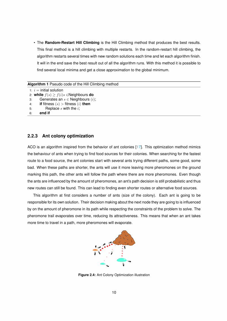
2.2.3 Ant colony optimization
ACO is an algorithm inspired from the behavior of ant colonies [17]. This optimization method mimics
the behaviour of ants when trying to find food sources for their colonies. When searching for the fastest
route to a food source, the ant colonies start with several ants trying different paths, some good, some
bad. When these paths are shorter, the ants will use it more leaving more pheromones on the ground
marking this path, the other ants will follow the path where there are more pheromones. Even though
the ants are influenced by the amount of pheromones, an ant’s path decision is still probabilistic and thus
new routes can still be found. This can lead to finding even shorter routes or alternative food sources.
This algorithm at first considers a number of ants (size of the colony). Each ant is going to be
responsible for its own solution. Their decision making about the next node they are going to is influenced
by on the amount of pheromone in its path while respecting the constraints of the problem to solve. The
pheromone trail evaporates over time, reducing its attractiveness. This means that when an ant takes
more time to travel in a path, more pheromones will evaporate.
Figure 2.4: Ant Colony Optimization illustration
10

Artificial bee colony algorithm
The Artificial bee colony (ABC) algorithm [18] is a metaheuristic that much like the Ant colony algorithm
tries to emulate the group behavior of, in this case, a colony of bees. In the real behavior of a Honey
Bee Swarm there are three main components of forage selection:
• Food Sources – In the food source, the forager bees evaluate several properties such as energy’s
quality, nectar’s taste, how close it is to the hive and the degree of difficulty of extracting energy
from this food source.
• Employed Foragers – Employed foragers are employed to the food source they are currently ex-
ploiting. These employed foragers carry the evaluation given to the food source they are employed
to. This information is then shared with the rest of the colony.
• Unemployed Foragers – An unemployed forager is a forager that does not get any food source
assigned to it. The goal of this bees is to explore the solution space randomly in an attempt to find
new food sources.
The algorithm first produces all food sources for all the employed bees. Then each bee travels to a
food source stored in her memory and when it arrives, it evaluates the food source’s quality. After this
the unemployed bees check all the information given by the employed bees and with a bias choose a
food source to neighbour. The best food source at any moment is always saved. This continues until all
criteria is met.
2.2.4 Genetic Algorithm
The Genetic Algorithm is a metaheuristic based on the process of natural selection. This algorithm
generates a population of solutions and from these solutions select several to reproduce and generate
offsprings for the following generation. The solutions that end up reproducing are usually the best
solutions, replicating natural selection, the survival of the fittest.
Initialization
The initialization is a step that is only made once n the beginning of the algorithm. It is when the
population is generated, usually it is generated a population with a size depending on the problem at
hand. This population is generated randomly. With this random solutions and with a big population the
probability of this population be spread as much as possible in the search space.
11

Fitness function
In this step the fitness value of each solution is calculated. The fitness function evaluates each solution.
It is really important to have a fitness function that represents the situation to optimize as close as
possible.
Selection
When in selection, the goal is to select the solutions that are going to be chosen to to generate new
offsprings.
There are several ways of selecting these solutions [19]:
• Proportionate Selection – this selection scheme, also known as roulette wheel selection, calcu-
lates the probability of every solution being chosen based on the value of its fitness.
• Tournament Selection – this method selects randomly a set of solutions and selects the ones
with the best fitness. Usually the number of individuals in each set is two but it is possible to have
greater tournaments. In the case of two solutions in one set, both are compared and then the best
out of them is chosen.
• Truncation Selection – this method is the most intuitive of them all because it ranks all of the
solutions based on their fitness and then it selects the best ranked.
• Elitist Recombination – in here, the method is a little more complex. It runs a small algorithm
with the goal of choosing the solutions to mate. It first initializes the population, then it shuffles
the population and forms mating pairs, each mating pair produces an offspring, the offspring is
evaluated and in the end only the best two of each family are saved.
Algorithm 2 Elitist Recombination Algorithm
1: initialize population2: for for every generation do3: generate offspring4: keep the best two of each family
Crossover
The crossover represents the set of points where it is selected in the parent chromosomes the informa-
tion is going to pass on to the offspring.
In a Single-point Crossover a point is previously defined or a point is randomly selected from the
chromosomes. This will lead to a swap of genes between both parents from the crossover point. When
12

there is more than one crossover point the procedure is the same but with more points, in this case it is
called a k-point crossover or a multi-point crossover.
Figure 2.5: Single-point Crossover (left) and k-point Crossover (right)
Also, unlike in most cases that happen in nature where both parents contribute with roughly the
same amount of genes, it is possible to have a mixing ratio different than 50%. When it is uniform it is
an uniform crossover, when it is not it is simply a non-uniform crossover.
Figure 2.6: Uniform Crossover (left) and Non-uniform Crossover (right)
Mutation
In nature, sometimes mutations happen from generation to generation. In the GA this phenomena
is replicated. Mutations are used to keep genetic diversity in the population. There is a very small
probability associated with the occurrence of this phenomenon.
Figure 2.7: Example of Mutation in a binary chromosome
13

Algorithm 3 Genetic Algorithm pseudocode1: set parameters2: initialize population3: while i < Number of Iterations do4: Fitness Calculation5: Selection6: Crossover7: Mutation8: end while9: return best solution =0
2.2.5 Exact Algorithms
These algorithms have this designation because their approach aims to find the optimal solution of every
optimization problem. So the core definition is that these algorithms always find the optimal solution. The
major problem with this algorithms is that they take to much of computational time and so they tend to
be only used in smaller problems. With the advances in the computational power and the amount of
problems where these exact algorithms can be applied it tends to increase.
In [20] an Exact Algorithm is used to solve a CVRP using Branch-and-Cut.
Branch-and-cut is an exact algorithm used to solve Integer Linear Problems (ILP). Branch-and-cut
is a Brunch-and-bound algorithm that uses cutting planes to reduce the number of possible solutions.
Once the algorithm ignores all of these solutions that were considered unfeasible or sub-optimal, it
saves a lot of time when trying to find the optimal solution. In Brunch-and-bound the algorithm starts by
creating a rooted tree that represents the state space search. In this tree the branches are compared
with lower and upper bounds that will help access if a branch is worth pursuing or not.
14
3Delivery Truck Assignment
In this case the transportation costs account for more than 50% of the total supply chain bill so it important
to have this part optimized.
Before explaining the proposed method, it is very important to see how the current model works
and how it is designed so to better understand what causes the main problems in efficiency and to
understand easier the methods that are going to be proposed and their main goals.
3.1 Current Transportation Model
In the current distribution model of Worten its routes or its calendar it is not adjusted according to the
business needs. This means that despite the changes on locations’ needs the distribution plan is more
or less the same throughout the year.
There are four main problem associated with the current model:
• Cost by full truckload – The cost of transportation is by full truckload. This means that the cost
paid for a truck is independent on the quantity of pallets inside of it, hence a truck being 50% full or
100% full has the same cost for the company. In the current transportation model the load factor is
15

Figure 3.1: Transportation model
around 75%. So, with this load factor it is easy to see that it is possible to save up to 25% of costs
in transportation with an optimized fleet.
• Handling Costs – These are referred to the costs of cargo preparation when loading a truck for
delivery. Just like in the previous case the cost is the same if the truck is full with cargo or not.
• Too much reliance on the transportation – The problem with having such a method of trans-
portation is its incapability of bending to the unexpected. If for some reason the if there is no
transportation in one day, this would cause delays in deliveries, and this could be very harmful on
the costumer’s eye.
• Lead Time – The Lead Time accounts for the time since the order has been made by the costumer
to the moment it reaches its final destination. If the products are mostly in a main warehouse
hundreds of km’s away, this is going to compromise the level of service.
Example
Let us suppose a scenario with five delivery days, where is necessary to transport fifty pallets for the
hub, twenty for store 1, thirty-seven for store 2, twenty-seven for store 3 and forty for store 4. It is known
that there are due dates for all the pallets and that the hub must be visited everyday.
A possible transportation schedule is shown in table 3.1:
Day
1
Day
2
Day
3
Day
4
Day
5
5 20 15 5 5 50 Hub
10 10 20 Store 1
15 20 35 Store 2
17 10 27 Store 3
20 20 40 Store 4
Table 3.1: Example of a week transportation schedule on the current model
16

Knowing that the capacity of the delivery trucks is fixed and equal to 33 it is possible to calculate the
average load rate of the trucks that are necessary to delivery during the week:
Day
1
Day
2
Day
3
Day
4
Day
5
35 52 15 35 35 172 Pallets per Day
2 2 1 2 2 9 Minimum trucks per Day
53% 79% 45% 53% 53% 58% Load Rate
Table 3.2: Load Rate in the Current Model
In the table above, 3.2, it is possible to check some of the problems with the current transportation
model. There is just 58% of load rate. If we divide the number of pallets to be delivered in this particular
week, per the cargo capacity of the trucks, 33, the lower bound on the number of vehicles that can satisfy
these requests is 6. In this example 9 trucks are allocated, 3 more than what is necessary.
3.2 Problem Approach
It is important to understand that a simple route optimization based on the total distance travelled would
be a naive approach once it would not take into account the weight each location has in the total demand
and it also ignores the due dates of the different locations.
The proposed approach is to check the demand of each store and the Hub every week. By knowing
the demand and the due dates of the each pallet, it is possible to get the dates when each pallet should
be delivered taking into account the total weekly demand of the cluster of locations, with the information
of what is delivered when it is possible to build the best routes for each day.
One of the first assumptions of this model is that is possible to stock pallets inside the Hub, with this
assumption it stops being mandatory to send trucks everyday to supply the Hub. Storing pallets at the
Hub can be beneficial but it has a cost, so a trade-off must be achieved. Another assumption says that
not only the pallets for the Hub can be delivered days before the due dates, but the pallets that have
stores as a destination can also arrive days before, with a storage cost associated also. The storage cost
between the Hub and the stores is going to be different. In this particular scenario it is less expensive to
store goods in the stores than to store in the Hub.
Another important assumption is that all locations inside a cluster can be visited in one route.
If this assumptions prove to be beneficial they can help to increase the Load Rate of the trucks thus
reducing the number of trucks needed every week – Cost by Full-Truck Load and Handling Costs.
17

Example
Let us suppose the same example showed in section 3.1 but with the new assumptions that were ex-
plained before. Here the Load Rate is increased by delivering pallets before the due date in the Hub.
Day
1
Day
2
Day
3
Day
4
Day
5
25 25 50 Hub
10 10 20 Store 1
15 20 35 Store 2
17 10 27 Store 3
20 20 40 Store 4
Table 3.3: Example of a week transportation schedule on the proposed model
The changes were that deliveries with Hub as destination delivered in Day 2 are now being delivered in
Day 1 and what had a due date in days 4 and 5 are now delivered in Day 3.
Day
1
Day
2
Day
3
Day
4
Day
5
55 32 25 30 30 172 Pallets per Day
2 1 1 1 1 6 Minimum trucks per Day
83% 97% 76% 91% 91% 87% Load Rate
Table 3.4: Load Rate in the Proposed Model
As it is possible to observe in the example above the Load Rate of the trucks as increased from 58%
to 87% by eliminating the rule that pallets should be delivered on their due dates. In this case only the
pallets with hub as destination were moved and the increase in overall results is already noted. The
trade-off in this scenario is that pallets will need to be stored in a more expensive place (hub), adding
an extra cost on the total operation. Taking into account this and other improvements it still might not be
feasible to achieve a 100% load rate.
3.3 Mathematical Formulation
At each week, the logistic system has a list of n pallets to deliver. A pallet, i, can be delivered in one of
the W days available for delivery and in one of the s vehicles available for delivery every day. This infor-
mation is given by a three-dimensional binary matrix xijk ∈ {0, 1},∀i ∈ {1, ...., n},∀j ∈ {1, ...., s},∀k ∈
{1, ....,W}. This matrix allows to see if a pallet i has been delivered by the vehicle j in the day k. The
day k given by xijk represents the completion date, which is the date the pallet i is delivered. There is a
18

list with a size of n× 1 that represents the due dates of each pallet. This list of due dates, D, is a list of
n pallets where di ∈ D and di ∈ {1,W}, this list represents the date when a pallet has to be delivered.
This due date list, D, is useful to check the delivery compliance when compared against the completion
date.
When it comes to assign pallets to days it is used an Assignment Problem. In the case case of
assigning the same pallets to trucks it is used a Capacitated Vehicle Routing Problem.
Capacitated Vehicle Routing Problem
As briefly mentioned in section 2.1.2 a CVRP is a typical VRP [9] with a limited capacity. In the CVRP
there is a set of m locations L = {l0, l1, l2, ..., , lm} and a set connections between these locations
C = {(vi, vj) : i 6= j} this can be represented. One of the locations in L represents the depot, l0, and
C represents the cost of transportation of a truck in full truckload between locations. In this formulation
there is a binary decision variable rtpq where the truck t ∈ {1, ..., s} is travels in the arc (i, j).
Assignment Problem
The Assignment Problem is a classic optimization problem that attempts to assign agents to tasks. In
the following formulation this assignment problem is constructed with a CVRP as explained before. The
goal is to minimize the global cost of the supply chain operation, assigning pallets to completion dates
while respecting all constraints.
19

minimizes∑
t=1
m∑p=1
m∑q=1,q 6=p
cpqrtqp +
W∑k=1
s∑j=1
CT +
n∑i=1
CiP (3.1)
subject tos∑
j=1
W∑k=1
xijk = 1 ∀i ∈ {1, ..., n} (3.2)
n∑i=1
s∑k=1
xijk ≤ sQ ∀j ∈ {1, ..., s} (3.3)
n∑i=1
xijk ≤ Q ∀j ∈ {1, ..., s},∀k ∈ {1, ...,W} (3.4)
s∑t=1
m∑p=1,i6=q
rtpq = 1 ∀j ∈ {1, ...,m} (3.5)
m∑j=1
rt0q = 1 ∀t ∈ {1, ..., s} (3.6)
m∑p=1,p6=q
rtpq =
m∑p=1
rtqp∀j ∈ {1, ...,m},
∀t ∈ {1, ..., s}
(3.7)
The objective function presented above, Equation (3.1), represents the typical CVRP formulation, its
goal is to minimize the total travel cost of all vehicles. This proposed solution daily evaluates the pallets
to deliver defined and solves a CVRP each day. The constraint presented in Equation (3.4) assures
that the total demand of each route does not exceed the capacity of each truck. In Equation (3.5) the
constraint that each location is visited once and once only is guaranteed. Equation (3.6) ensures that
a truck can leave the depot once. The equation represented by (3.7) defines that the number of trucks
entering in each location, depot included, is equal to the number of trucks leaving the depot.
The transportation costs are seen in two ways, the cost of vehicle preparation, also called cost of
service, CSV , and a cost per vehicle, CV . The CV represents an average cost of using a vehicle. Both
values are constants for every vehicle.
CT = CSV + CV (3.8)
According to Pinedo [21], the lateness of a job is given by Li = oi−di. It is assumed that it is possible
to deliver orders with days to spare, Li < 0, on the due date, Li = 0, and to deliver orders after the due
date Li > 0. For Home Delivery of Large Formats (HDLF), when Lj 6= 0, there is a penalty cost, CiP ,
associated with them. In the case of Li < 0, there is a Cost of Storage, Cs. This is the cost associated
with the order being stopped in an advanced warehouse in the Supply Chain. In the case of Li > 0,
there is a Cost of Lead Time, CLT . This is the cost associated with the order not being delivered on
20

time.
CPi =
|Li|Cs, Li < 0|Li|CLT , Li > 0
0, Li = 0(3.9)
21

22
4Proposed Methods
As it can be seen in the previous sections, there are several possible algorithms that could be applied
in the chapter 3. In this case it is proposed to use a Genetic Algorithm (GA) and/or a Local Search
Algorithm (LSA) to solve the problem. The reason for this choice is because in most SCM optimization
problems both GA and LSA are the most used algorithms. Besides the fact of being algorithms broadly
chosen, as it is referred in section 2.2.4, they are algotihms that usually get to high-quality results.
Another reason was the ease of implementation f both algorithms and their speed getting good results
4.1 Initial Solution
The first step in order to find the solution that better fits the problem at hand is building an initial solution
from which the algorithm is going to be computed. In both Genetic and Local Search algorithms an
initial solution is randomly created. It is possible to use random generated solutions because in this
problem all possible combinations are considered as valid. For every solution it is presented a vector
with n elements where each element represents a pallet to be delivered, the number of each element
represents when a pallet is to be delivered.
23

In the GA, the randomly generated solutions will allow to have more diversity within the initial popu-
lation, increasing the probability of finding better solutions. In the Local Search Algorithm this randomly
generated solutions allow for different starting conditions while performing an Iterated Local Search Al-
gorithm.
Figure 4.1: ”Family” of solutions in a GA (left) vs solution in LS Algorithm (right)
4.2 Evaluation
There are two different methodologies in the Evaluation Function (EF), both of these evaluation functions
are going to be used in the three algorithms proposed. In one EF method the transportation cost is going
to be evaluated with a high level of precision while the other method will use an estimate. The advantage
of the later is its computing speed. In both methods the EF starts by saving the pallets that are going
to be delivered each day. With that information it is also possible to get the locations that are going to
be visited in each day and also the total amount of pallets to deliver everyday. Below can be seen an
example where a solution is evaluated. The solution used in this example is the following:
[ 2 2 1 2 1 3 3 3 1 1 1 5 5 5 4 5 4 2 4 ]
In the example above it is possible to see the evaluation process starting by sorting the pallets to the
days of delivery (the first element of the example’s solution has a value of 2, therefore the pallet number
1 is delivered on day 2). One of the information given as input is which pallets are delivered in each
location. With the information of which pallets are delivered it is possible to know the locations to visit in
24

Figure 4.2: Example of the evaluation process
each day. By knowing, per day, the locations to visit and the number of pallets per location it is possible
to use that information as input for the CVRP and compute the optimal routes per day.
4.2.1 Capacitated Vehicle Routing Problem
The Capacitated Vehicle Routing Problem (CVRP) in this case is implemented using CPLEX. CPLEX is
an optimization software that allows a simple integration of Mixed Integer Linear Programming (MILP)
problems in Python.
The CVRP as described in section 3.3 will use the route distances is using the euclidean distance
between the locations instead of using the real road distance due to the computational time.
Figure 4.3: Euclidean Distance (Blue) and Driving Distance (Red)
In-Evaluation
When the EF has an In-Evaluation method this means that an exact algorithm for the CVRP is done
everytime the EF is called. This allows the EF to be more precise when calculating the cost of each
solution. The main problem with this approach is the time factor. Because a CVRP is solved for every
25

solution the increase in computing time may not justify the improvement on the quality of the solution.
In this method the quantities to be delivered per location per day are given to the CVRP so it is
possible to know the best possible routes for the given demand.
Out-Evaluation
The other approach, called Out-Evaluation, as the name suggests performs the exact algorithm outside
the EF. In this case the algorithm only uses an estimate as transportation costs. This method aims to
be much faster than the In-Evaluation method, but it is not as sensitive during the process of finding
solutions.
In this method the only the quantities to be delivered per location per day of the last solution, the
optimal solution, are given to the CVRP. So, only after the optimization of days assignment is done the
routes are known.
Figure 4.4: In-Evalutation (left) vs Out-Evaluation (right)
4.3 Genetic Algorithm
The Genetic Algorithm (GA) applied in this thesis is an optimization algorithm used to solve combinatorial
problems with a big solution space. This algorithm is used due to getting fast and good solutions. How
26

this algorithm works is already explained with more detail in section 2.2.4. In this section it is going to
be explained how GA is applied to this problem.
Gene
To start this algorithm it is necessary to find a chromosome that represents in the best way possible the
potential solutions of the problem. This chromosome not only needs to represent well the problem, but
it also needs to be in a format that allows for a fast evaluation process.
The used chromosome is a vector with a size corresponding to the number of deliveries. In this chro-
mosome, each gene represents a pallet and the value of each gene is the day each pallet is delivered.
Figure 4.5: Chromosome
Figure 4.6: Applied example for the chromosome for 6 pallets
In the example above the pallet number one is to be delivered on day 2, pallet number two is to be
delivered on day 1, pallet number three is to be delivered on day 5, pallet number four is to be delivered
on day 3, pallet number five is to be delivered on day 2 and pallet number six is to be delivered on
day 5. This gene allows for a simple understanding of the solution, an easy generation of new possible
solutions and it also allows for easy crossover and mutation operations.
Crossover
The crossover is the used method for generating new solutions from a previous population. It is a natural
selection-based process that takes the genes from other solutions (parents) and generates new ones
(offsprings).
Usually, when choosing the parents, the genes that are going to give the chromosomes to generate
new solutions, the fitness of the gene is considered. The genes with the best fitness have higher proba-
bility to be chosen to generate new solutions. In this case it is going to be attempted a different approach
and instead of looking at the fitness of the individual solutions, the goal is to look at the difference be-
tween the solutions in comparison with the remaining solutions of the population. This will allow for an
higher diversity of solutions, for a better search and it will also be less likely to have a the algorithm stuck
in local minima.
27

In this case it is going to be applied an uniform multi-point crossover. This means that the same
amount of information is used from different chromosomes when creating a new chromosome.
This crossover is made by combining pairs of solutions and performing a multi-point crossover be-
tween each other. The pairing of solutions is done randomly from the most diverse solutions.
Mutation
The mutation process used in this GA is similar to the one previously described. The mutation is possible
for every gene, this selection is done at random and the probability for each gene to be mutated is also
pre-defined.
A small algorithm that describes the mutation process is presented:
Algorithm 4 Mutation
1: A probability for the mutation to occur is given2: if chromosome is selected then3: Selects a random gene4: Randomly changes the value of the gene to another feasible value5: return Genetically modified chromosome
In the following example a chromosome has been randomly chosen to be mutated. After this selec-
tion, a gene in the chromosome is also chosen at random and it is going to be replaced by a different
feasible gene. A feasible gene is a gene which all its values are feasible, i.e., all values respect the
constraints given.
Figure 4.7: gene mutation process
Selection
The process described in this subsection is the responsible for the selection of chromosomes that go
from one generation to the other. There are several methods to perform this operation as it can be seen
in previous sections. In this case it several methods are combined.
28

To select half of the population that progresses to the next generation it is used a proportionate
selection, most commonly known as roulette wheel selection. In this case, from the pool of solutions
generated by the parents of the previous generation, the solutions with the better fitness have a higher
chance of being chosen to the next generation. To get the other missing half of the next generation’s
population, the corresponding number of new solutions are created. This allows for new information to
come into the pool of solutions and increase diversity. There is also elitism, because the best solution of
each generation is always going to the next.
Figure 4.8: Selection Process
Pseudo-Code Genetic Algorithm
Algorithm 5 Genetic Algorithm for Delivery Truck Assignment for SCM
1: Generates an initial population of feasible solutions2: for Number of Iterations do3: Evaluates the Fitness of each solution4: Saves the best solution to go to the next generation (Elitism)5: Selects the top most diverse solutions to reproduce (Parents)6: The Parents randomly reproduce generating new solutions (Offsprings)7: Half of the next generation is selected from the pool of offsprings8: Half of the next generation minus one is randomly generated9: return Optimized Solution
29

4.4 Local Search Algorithm
The Local Search (LS) is an algorithm that improves the current solution by exploring its neighboring
space. It is a very simple algorithm to explain and to implement. In this implementation it is going to be
used the Hill Climbing (HC) algorithm.
The HC agorithm is an algorithm that continuously tries to improve the fitness value of the solution.
In this case it works in a minimization problem, where it is attempted to find the minimum of the cost
function, so the HC algorithm finds solutions that decrease the fitness value of each solution until it
reaches a point where there is no neighboring solution with a lower fitness value, this point is also called
local minima. When the HC algorithm reaches local minima it stops iterating.
As there is no way of knowing if the local minima corresponds to the global minima, in this approach
it is done an Iterated Local Search. An Iterated Local Search runs the algorithm several times in an
attempt of finding different solutions of local minima, therefore increasing the chances of finding the
optimal solution of the problem.
Algorithm 6 Local Search Algorithm for Delivery Truck Assignment for SCM
1: An unique solution is generated2: while Solution does not reach a local minima do3: The day of delivery is changed4: if chromosome is selected then5: Selects a random gene6: Randomly changes the value of the gene to another feasible value7: return Genetically modified chromosome
4.5 Exact Algorithm
The Branch-and-Cut Algorithm always gives the optimal result and with its cutting planes helps to tighten
the state space of solutions hence reducing the total computing time.
In this case the Branch-and-Cut Algorithm will only be used to compute the best transportation cost
in each scenario previously defined, solving a CVRP. This is, it will receive as input the locations to
deliver pallets and how many to deliver per day, then it will compute an optimal route for each day. The
reasoning behind using this algorithm in this CVRP is the reduced number of possible locations and
number of pallets.
30

4.6 Hybrid Algorithm
In this implementation of an Hybrid Algorithm it is attempted to merge the best the genetic algorithm has
with the best of the local search algorithm. As the weights of the deciding factors have high differences
it is easier to have the GA stopped in a Local Minima. It is then assumed that in the first iterations the
GA will have advantages over the LSA, since it evolves faster in the beginning. When the benefits of the
GA stop, when it starts reaching local minima, the LSA is better once it searches in the neighborhood of
its solution.
With this in mind, the Hybrid Algorithm proposed in this thesis will use the GA as a first solution
generator for the LSA. This solution allows to have the best of each algorithm, in the GA, the fast
initialization, and with the LSA the ability to find new solutions in the neighbourhood.
Algorithm 7 Hybrid Algorithm for Delivery Truck Assignment for SCM
1: Generates an initial population of feasible solutions2: for Number of Iterations do3: Evaluates the Fitness of each solution4: Saves the best solution to go to the next generation (Elitism)5: Selects the top most diverse solutions to reproduce (Parents)6: The Parents randomly reproduce generating new solutions (Offsprings)7: Half of the next generation is selected from the pool of offsprings8: Half of the next generation minus one is randomly generated1: return Optimized Solution2: while Optimized Solution does not reach a local minima do3: The day of delivery is changed4: if chromosome is selected then5: Selects a random gene6: Randomly changes the value of the gene to another feasible value7: return Genetically modified chromosome
4.7 Brief software explanation
The programming of the algorithm presented in the previous chapter was made in Python. This pro-
gramming was divided in 6 main parts:
• Data Import - In this function the data is imported from the datasource. It is from this datasource
that the number of pallets to deliver, the days of delivery, the coordinates of each location and the
costs or penalty values come from.
• Initialization - In Initialization is where the first solution is created. In the Local Search Algorithm,
only a vector that corresponds to the first solution is created. In the Genetic Algorithm several
vectors are created with the same format each corresponding to a member of the first generation
of the population.
31

• Evaluation - Each solution is evaluated individually. In Evaluation it is seen when each pallet s
going to be delivered, the number of pallets to deliver each day, the locations to visit each day and
then the minimum required number of vehicles needed per day. It is also in this function that the
penalties are awarded to each solution, this penalties are the ones related to storage days and
delay days. In the end of this function all of these factors are combined to give a cost for each
solution.
• Local Search Algorithm - This function receives the vector that represents the current solution
and starts by iterating each value of the vector in order and every time the solution is improved it
moves to the next value, when it reaches the end of the vector it starts over until there are no more
possible moves.
• Genetic Algorithm - It starts by creating a population, then each chromosome is evaluated and
ranked. The best solutions will be selected as parents. In this algorithm, the number of parents
mating will be half of the population size to grant the most diversity possible when generating
offsprings. Half of the new population is newly created and the other half minus one (the best
solution) is selected randomly from the offsprings pool.
• CVRP - This algortihm uses the information of the number of pallets to be delivered per day and
what locations are visited to build the most cost-effective routes. Its output ends up being the
routes taken and the number of vehicles needed.
32

5Results and Discussion
The results of the previously described algorithms are presented in this chapter. These models are
tested and compared against each other. In the beginning of this chapter the general structure of the
input data is given. Then, for the Genetic Algorithm (GA) a sensibility analysis is done to find what are
the best parameters to be used in this problem. After the parameterization is done the final results for
the GA will be compared against the remaining different methods, LSA and Hybrid Algorithm.
5.1 Demand data
In order to test the algorithms in different conditions it is important to verify the algorithm in different
conditions because the demands are highly influenced by seasonality, and it is necessary to ensure
that the algorithm works for the entire year. These solutions are inspired by typical business weeks
of Worten’s year, and closely represent the demand volume and the amount of locations to visit per
region. This representation used historical data to forecast the demand value in the region of Valencia
in Spain. To test the strength of the algorithm, besides the realistic values on this particular case study,
the algorithm is going to be also tested in critical conditions. This strength test is going to act on the
33

demand and on the number of locations to visit. It is going to be tested a case with much less demand
than what is expected, and the opposite, much more demand than expected. The number of locations
is also going to suffer the same test.
5.2 Data analysis
In this section it is going to be analysed some data in order to build the baseline problems to be solved.
The goal of using several benchmarks is to evaluate different characteristics on the algorithms. This
characteristics are the ability of handling different volumes of pallets every week or the need to deliver
to different number of locations. There were 9 solutions build for this purpose. A solution with a low,
another with the usual and finally one with a high weekly demand. For each of these solutions it was
tested a low, an usual and a high number of locations to visit per week. The algorithms will be evaluated
based on their best solution and on the time needed to reach the local minima.
To build this baseline problems some rules were used. This rules were based on the company’s
historical data. It was possible to see that most home deliveries are due to Tuesday and Wednesday,
very few are due to Monday, and the remainders are due to Thursday and Friday. Also it is possible to
see that currently around 30% of the deliveries are Home Delivery.
• There are 6 days of delivery (Monday, Tuesday, Wednesday, Thursday, Friday and Saturday)
• 30% of the weekly demand is for Home Delivery
• 33% of the Home Delivery is due Tuesday
• 33% of the Home Delivery is due Wednesday
• 17% of the Home Delivery is due Tuesday
• 17% of the Home Delivery is due Wednesday
There is also going to be build some baseline problems with a wider solution space. The increasing
size of the solution space will be obtained in a scenario where most deliveries have due dates for the
end of the week while some maintain the need to be delivered in the beginning of the week. Such
scenarios are possible in targeted promotion campaigns for the weekends and in Black Friday. In this
circumstances the stores would need their regular supply plus the added supply for the end of the week.
The increase in the solution space size would happen once there would be more pallets to deliver in
the end of the week and this would result in a greater number of possible days to deliver. For instance,
since it is not considered delay, a pallet that needs to be delivered until Friday, can be delivered Monday,
Tuesday, Wednesday, Thursday and Friday, whilst a pallet to be deliver on a Monday only has that one
34

option. Hence, with a proportionally higher number of pallets to be delivered in the end of the week,
there is a higher number of possible solutions.
In the following sections it will be shown the results of a particular case where the space of solutions
is much larger. This case will represent a harder problem to solve where the amount of possible solutions
is increased. This scenario will represent cases when it is expected much more sales on the end of the
week (Fridays and weekends). In this scenario the distribution is the same as above, but the stores
supply is due to later in the week.
5.3 Parameter Configuration
For the Genetic Algorithm and the Hybrid Algorithm it is necessary to do a parameter configuration.
In this process, several parameters are chosen based on the influence they have on the algorithm’s
performance. In this section the parameters that will be studied are the number of chromosomes in the
population and the relationship between the number of chromosomes and the number of offsprings. It
is also going to be seen the optimal number of generations needed and also the number of crossover
points.
5.3.1 Population size and number of offsprings
The first parameter to be chosen will be the population size and the number of offsprings that will
come from the population. This parameters will be selected together because they are dependent upon
each other, this is, the number of offsprings generated is connected with the size of the population
once it comes from it. It is going to be presented bellow a table with the mean results of several each
corresponding combination of parameters. It is known that as the population size and the number of
offsprings increase the computing time will also be higher due to the increased number of chromosomes
to evaluate. This factor will also be important on evaluating the best parameters once if the difference
between two options is not significative then the one with the lower running time will be chosen. The
offspring-population ratio tested range will be from 0.5 to 2 and the population size will be from 50 to
500.
Offsprings/PopulationPopulation 0.5 1 1.5 2
50 7593 7596 7596 7647100 7599 7656 7563 7551250 7542 7581 7575 7545500 7554 7551 7503 7569
Table 5.1: Offspring and Population number selection
35

In the previous table the best solution is given by the (500,1.5) combination, hence this were the
parameters chosen. This means that for the GA and he Hybrid Algorithm the population size will be of
500 chromosomes and the number of offsprings generated will be 1.5 times that, 750 offsprings.
5.3.2 Number of crossover points
To select the number of crossover points several values are tested. To choose the best value for the
number of crossover points the selection will be based on the best generated results. It is going to be
tested for a range of values from 1 to 80.
Crossover Points 1 2 5 10 20 40 807578 7545 7554 7536 7575 7566 7569
Table 5.2: Number of crossover points selection
As it can be seen it the table above the number of crossover points that resulted in the best solution
was 10 crossover points, so it is the value used from now on.
5.3.3 Number of generations
In this parameter it is going to be selected a different value to the GA and to the Hybrid once it has
different proposes in both cases. In the first the goal is to reach the best solution possible while in the
other the goal is to advance the result the most for the LSA.
To select the number of generations in the GA the algorithm is run several times with a high number
of generations to to see where the GA gets in a local minima. In the Hybrid algorithm the principle will
be to check a number of iterations that improves he first solution for the LSA, hence, the same analysis
will be used.
The algorithm was tested several times with 1000 generations, in an attempt to see the values where
it stopped having a significant increase in its fitness result.
As it is possible to see in the figure above, after the 100th iteration the result stopped improving
significantly. With that in mind the number of generations in the GA was defined as 100.
5.4 Results
In the following sections the results of each of the proposed algorithms will be analysed and in the end
compared against each other. The first algorithm will be the LSA, then the GA and finally the Hybrid
approach designed to minimize the issues of each of the previous two and improve performance. In this
sense all of the algorihtms will be tested under the same conditions.
36

Figure 5.1: Genetic Algorithm 1000 iterations
5.4.1 Local Search Algorithm
In this section it will be evaluated the results produced by the LSA alone. Both approaches, In-Evaluation
and Out-Evaluation will be compared for this algorithm.
In-Evaluation
Figure 5.2: Local Search Algorithm In-Evaluation
Out-Evaluation
As expected, the approach where it is used the routing inside of the evaluation function it takes about
eighty times more time to get the final results, but it gets much better results.
37

Figure 5.3: Local Search Algorithm Out-Evaluation
5.4.2 Genetic Algorithm
In-Evaluation
Figure 5.4: Genetic Algorithm In-Evaluation 100 iterations
Out-Evaluation
By observing the results of both of these approaches it is possible to say that the parameters chosen in
the previous section were not ideal. The first iteration gives good results, but for the GA to keep improving
more and more it would need a bigger population. The problem with having a bigger population is the
computing time. That is why, in the following section it is attempted to use the GA in the first iterations
(using a bigger population) and use the final result as the first solution for the LSA.
38

Figure 5.5: Genetic Algorithm Out-Evaluation 100 iterations
5.4.3 Hybrid Algorithm
In-Evaluation
Figure 5.6: Hybrid Algorithm In-Evaluation
Out-Evaluation
In the first attempt of building a Hybrid Algorithm the number of generations used was 5, and despite
the low number of generations it is possible to see that each generation took about 100 seconds each,
taken almost 50% of the overall computing time. In this sense it was attempted a second approach with
only 2 generations to see if it would improve the overall result against the solo LSA.
39

Figure 5.7: Hybrid Algorithm Out-Evaluation
Second hybrid attempt
In-Evaluation
Figure 5.8: Hybrid Algorithm In-Evaluation
Out-Evaluation
With this results it is possible to say that the computing time was significantly reduced compared with
both LSA and the first approach of the Hybrid Algorithm. The final results were more or less the same
between all of these algorithms.
40

Figure 5.9: Hybrid Algorithm Out-Evaluation
5.5 Discussion
5.5.1 Final Results
In-Evaluation
GA LSA HA Real ResultsCost(e) 7870 6418 6433Time(s) 4616 920 529
Table 5.3: Results In-Evaluation
Out-Evaluation
GA LSA HA Real ResultsCost(e) 8698 7428 7428Time(s) 63 10 9
Table 5.4: Results Out-Evaluation
5.5.2 In-Evaluation vs Out-Evaluation
By comparing the results of both algorithms it is possible to see the main differences between each other.
When the In-Evaluation is performed the algorithm takes much longer to evaluate each solution and this
results in a much bigger duration of the algorithm, in spite of that it clearly produces better results due
to the fact that when it is making the decisions it worries about the exact paths the trucks need to take in
41

order to make the deliveries. In the Out-Evaluation it is much faster since it only calculates roots for the
best solution in therms of storage time and does not take into account the need of joining pallets that go
for the same locations in the same days of delivery or in the same trucks.
5.5.3 LSA vs GA vs Hybrid
In these algorithms it is possible to see that the better approach was the Hybrid Agorithm. The reason
for it is the fact that it minimizes the limitations of both the GA and the LSA. In the LSA algorithm the
first solution is randomly generated, so there is no criteria when it starts. With this randomly generated
solution the algorithm takes longer to reach an acceptable value for the cost function. While in the GA
the algorithm is fast to reach a good improvement in the first generation but it stops in local minima very
easily. Hence, by using the GA to start and as a way to compute the LSA first solution, it increases the
performance of both.
42

6Conclusions
In this master thesis a method to allocate orders both in time (days of the week) and trucks (the routes).
This method was constructed in a way that solved a real problem of the company Worten but that can
be applied to any retail company that has several deliveries to do per week and several destinations.
This method has the ability to improve the results currently achieved by the company if applied once it
adjusts the major supply chain decisions based on the demands given. One of the main focus when
building a solution was the computing time, and it was successful in this regard once it allows for when
sudden changes in planning happen to use the algorithm to build new solutions in time.
In the results it was possible to see that the LSA gave better solutions than the GA with less com-
puting time and the Hybrid approach marginally improved the solutions and shortened the computing
time.
The reason the GA was so ineffective was due to its need to compute the cost of too many solutions.
This increased its computing time too much and it was not possible to use a better GA due to this
restriction. This is one the reasons the Hybrid Algorithm worked better because it used slightly different
parameters that improved its performance (bigger population) and then the LSA where it focused on one
solution at a time.
43

Overall the approach in this thesis is able to solve delivery in supply chain problems in another
dimension that was covered just by typical VRPs.
6.1 Future Work
The proposed method can be improved and studied further in several ways. One of the ways this method
can be explored is by trying a different approach when hybridizing the algorithm. It can be attempted in
between the In-Evaluation and Out-Evaluation methods showed here. This would allow for the routing
algorithm to be only run a few times which would decrease the computing time significantly. With the
decrease of computing time, the parameters of the GA could be tuned hence improving its performance.
44

List of Tables
3.1 Example of a week transportation schedule on the current model . . . . . . . . . . . . . . 16
3.2 Load Rate in the Current Model . . . . . . . . . . . . . . . . . . . . . . . . . . . . . . . . . 17
3.3 Example of a week transportation schedule on the proposed model . . . . . . . . . . . . . 18
3.4 Load Rate in the Proposed Model . . . . . . . . . . . . . . . . . . . . . . . . . . . . . . . 18
5.1 Offspring and Population number selection . . . . . . . . . . . . . . . . . . . . . . . . . . 35
5.2 Number of crossover points selection . . . . . . . . . . . . . . . . . . . . . . . . . . . . . . 36
5.3 Results In-Evaluation . . . . . . . . . . . . . . . . . . . . . . . . . . . . . . . . . . . . . . . 41
5.4 Results Out-Evaluation . . . . . . . . . . . . . . . . . . . . . . . . . . . . . . . . . . . . . . 41
45

46

List of Figures
1.1 Comparison the number of stores in Portugal and in Spain . . . . . . . . . . . . . . . . . . 2
1.2 Normalized typical demand curve during a year in weeks . . . . . . . . . . . . . . . . . . 3
2.1 (A) Workflow in a Warehouse in Siemens Tecnomatix FactoryFlow (B) Layout of a Ware-
house (right) . . . . . . . . . . . . . . . . . . . . . . . . . . . . . . . . . . . . . . . . . . . 7
2.2 Bin Before and After Optimization . . . . . . . . . . . . . . . . . . . . . . . . . . . . . . . . 7
2.3 TSP vs VRP [14] . . . . . . . . . . . . . . . . . . . . . . . . . . . . . . . . . . . . . . . . . 8
2.4 Ant Colony Optimization illustration . . . . . . . . . . . . . . . . . . . . . . . . . . . . . . . 10
2.5 Single-point Crossover (left) and k-point Crossover (right) . . . . . . . . . . . . . . . . . . 13
2.6 Uniform Crossover (left) and Non-uniform Crossover (right) . . . . . . . . . . . . . . . . . 13
2.7 Example of Mutation in a binary chromosome . . . . . . . . . . . . . . . . . . . . . . . . . 13
3.1 Transportation model . . . . . . . . . . . . . . . . . . . . . . . . . . . . . . . . . . . . . . . 16
4.1 ”Family” of solutions in a GA (left) vs solution in LS Algorithm (right) . . . . . . . . . . . . 24
4.2 Example of the evaluation process . . . . . . . . . . . . . . . . . . . . . . . . . . . . . . . 25
4.3 Euclidean Distance (Blue) and Driving Distance (Red) . . . . . . . . . . . . . . . . . . . . 25
4.4 In-Evalutation (left) vs Out-Evaluation (right) . . . . . . . . . . . . . . . . . . . . . . . . . . 26
4.5 Chromosome . . . . . . . . . . . . . . . . . . . . . . . . . . . . . . . . . . . . . . . . . . . 27
4.6 Applied example for the chromosome for 6 pallets . . . . . . . . . . . . . . . . . . . . . . 27
4.7 gene mutation process . . . . . . . . . . . . . . . . . . . . . . . . . . . . . . . . . . . . . . 28
4.8 Selection Process . . . . . . . . . . . . . . . . . . . . . . . . . . . . . . . . . . . . . . . . 29
5.1 Genetic Algorithm 1000 iterations . . . . . . . . . . . . . . . . . . . . . . . . . . . . . . . . 37
5.2 Local Search Algorithm In-Evaluation . . . . . . . . . . . . . . . . . . . . . . . . . . . . . 37
5.3 Local Search Algorithm Out-Evaluation . . . . . . . . . . . . . . . . . . . . . . . . . . . . 38
5.4 Genetic Algorithm In-Evaluation 100 iterations . . . . . . . . . . . . . . . . . . . . . . . . 38
5.5 Genetic Algorithm Out-Evaluation 100 iterations . . . . . . . . . . . . . . . . . . . . . . . 39
47

5.6 Hybrid Algorithm In-Evaluation . . . . . . . . . . . . . . . . . . . . . . . . . . . . . . . . . 39
5.7 Hybrid Algorithm Out-Evaluation . . . . . . . . . . . . . . . . . . . . . . . . . . . . . . . . 40
5.8 Hybrid Algorithm In-Evaluation . . . . . . . . . . . . . . . . . . . . . . . . . . . . . . . . . 40
5.9 Hybrid Algorithm Out-Evaluation . . . . . . . . . . . . . . . . . . . . . . . . . . . . . . . . 41
48

Bibliography
[1] D. Grewal and M. Levy, “Emerging issues in retailing research,” Journal of retailing, vol. 85, no. 4,
pp. 522–526, 2009.
[2] R. M. Monczka, R. B. Handfield, L. C. Giunipero, and J. L. Patterson, Purchasing and supply chain
management. Cengage Learning, 2015.
[3] L. Aburto and R. Weber, “Improved supply chain management based on hybrid demand forecasts,”
Applied Soft Computing, vol. 7, no. 1, pp. 136–144, 2007.
[4] M. Zhang, R. Batta, and R. Nagi, “Modeling of workflow congestion and optimization of flow routing
in a manufacturing/warehouse facility,” Management Science, vol. 55, no. 2, pp. 267–280, 2009.
[5] K. J. Roodbergen and I. F. Vis, “A model for warehouse layout,” IIE transactions, vol. 38, no. 10, pp.
799–811, 2006.
[6] S. Martello and P. Toth, “Bin-packing problem,” Knapsack problems: Algorithms and computer im-
plementations, pp. 221–245, 1990.
[7] K. Kang, I. Moon, and H. Wang, “A hybrid genetic algorithm with a new packing strategy for the
three-dimensional bin packing problem,” Applied Mathematics and Computation, vol. 219, no. 3,
pp. 1287–1299, 2012.
[8] M. Diaby, “The traveling salesman problem: a linear programming formulation,” arXiv preprint
cs/0609005, 2006.
[9] P. Toth and D. Vigo, Vehicle routing: problems, methods, and applications. SIAM, 2014.
[10] ——, “Models, relaxations and exact approaches for the capacitated vehicle routing problem,” Dis-
crete Applied Mathematics, vol. 123, no. 1-3, pp. 487–512, 2002.
[11] H. Min, “The multiple vehicle routing problem with simultaneous delivery and pick-up points,” Trans-
portation Research Part A: General, vol. 23, no. 5, pp. 377–386, 1989.
49

[12] M. Desrochers, J. Desrosiers, and M. Solomon, “A new optimization algorithm for the vehicle routing
problem with time windows,” Operations research, vol. 40, no. 2, pp. 342–354, 1992.
[13] M. Gendreau, G. Laporte, C. Musaraganyi, and E. D. Taillard, “A tabu search heuristic for the
heterogeneous fleet vehicle routing problem,” Computers & Operations Research, vol. 26, no. 12,
pp. 1153–1173, 1999.
[14] W.-Y. Liu, C.-C. Lin, C.-R. Chiu, Y.-S. Tsao, and Q. Wang, “Minimizing the carbon footprint for the
time-dependent heterogeneous-fleet vehicle routing problem with alternative paths,” Sustainability,
vol. 6, no. 7, pp. 4658–4684, 2014.
[15] C. A. Silva, J. Sousa, T. A. Runkler, and J. S. Da Costa, “Distributed supply chain management
using ant colony optimization,” European Journal of Operational Research, vol. 199, no. 2, pp.
349–358, 2009.
[16] P. J. Brockwell, R. A. Davis, and M. V. Calder, Introduction to time series and forecasting. Springer,
2002, vol. 2.
[17] M. Dorigo and M. Birattari, Ant colony optimization. Springer, 2010.
[18] D. Karaboga and B. Akay, “A comparative study of artificial bee colony algorithm,” Applied mathe-
matics and computation, vol. 214, no. 1, pp. 108–132, 2009.
[19] D. Thierens and D. Goldberg, “Convergence models of genetic algorithm selection schemes,” in
International Conference on Parallel Problem Solving from Nature. Springer, 1994, pp. 119–129.
[20] N. R. Achuthan, L. Caccetta, and S. P. Hill, “An improved branch-and-cut algorithm for the capaci-
tated vehicle routing problem,” Transportation Science, vol. 37, no. 2, pp. 153–169, 2003.
[21] M. Pinedo, Scheduling. Springer, 2012, vol. 29.
50

51