demand for secondhand goods and consumers’ … and a basic questionnaire survey. thus, we obtained...
TRANSCRIPT

DPRIETI Discussion Paper Series 15-E-135
Demand for Secondhand Goods and Consumers' Preference in Developing Countries:
An analysis using the field experimental data of Vietnamese consumers
HIGASHIDA KeisakuKwansei Gakuin University
Nguyen Ngoc MAIHanoi Foreign Trade University
The Research Institute of Economy, Trade and Industryhttp://www.rieti.go.jp/en/

IETI Discussion Paper Series 15-E-135
December 2015
Demand for Secondhand Goods and Consumers’ Preference in Developing Countries:
An analysis using the field experimental data of Vietnamese consumers1
HIGASHIDA Keisaku
School of Economics, Kwansei Gakuin University
Nguyen Ngoc MAI
Faculty of International Economics, Hanoi Foreign Trade University
Abstract
Using the data from a series of field experiments that were carried out in in Hanoi, Thai Ping, and
Thai Hong in Vietnam, we examined the relationship between consumers’ preference for secondhand
products and consumers’ and products’ attributes. In particular, we extracted their risk, time, and
social cooperative preferences through the experiments. In addition, we surveyed their personal
attributes and conducted a type of conjoint questionnaire about motorbikes and fridges. Regarding
product attributes, we focused on the age, brand, size, quality labeling, origin, and so on. We found
that product attributes influence consumer utility as expected. For example, the Honda brand
positively influences consumer utility. Moreover, we obtained several important results about the
relationship between personal attributes and demand, in particular, about preference for secondhand
products. For example, consumers who are more far-sighted and/or older have stronger preference for
secondhand goods compared with the less far-sighted and/or younger consumers; the older and/or
male consumers have stronger preference for Japanese brands as compared with the younger and/or
female consumers. It is also possible that environmental consciousness affects the preference for
secondhand products. We also provide policy implications on quality certification and international
trade of secondhand goods. Keywords: Consumer behavior, Field experiment, Secondhand goods, Time preference
JEL classification: C93, Q53, Q56.
RIETI Discussion Papers Series aims at widely disseminating research results in the form of professional
papers, thereby stimulating lively discussion. The views expressed in the papers are solely those of the
author(s), and neither represent those of the organization to which the author(s) belong(s) nor the Research
Institute of Economy, Trade and Industry.
1This study is conducted as a part of the Project “Research on Trade/Foreign Direct Investment and the Environment/Energy” undertaken at Research Institute of Economy, Trade and Industry(RIETI). The authors are grateful for helpful comments and suggestions by Ryuhei Wakasugi, Tsuyoshi Kawase, Naoto Jinji, Morihiro Yomogida and Discussion Paper seminar participants at RIETI. The authors also acknowledge the financial support from Japan Society for the Promotion of Science under Grant-in-Aid for Scientific Research (B 26285057 ).

2
1. Introduction
Consumers often face choices between new and secondhand goods when they purchase
durables, such as cars, motorbikes, fridges, TVs, and personal computers. Some consumers
always buy new goods, while other consumers often buy secondhand goods. In some
countries, people are reluctant to purchase secondhand goods only because the products are
secondhand, while in other countries the fact that a product is secondhand is just one of the
several product attributes.
In particular, consumers in developing countries are more likely to buy secondhand
goods than those in developed countries when we compare their consumption behaviors on a
product coming from the same category. As such, the supply of secondhand goods is greater
than the demand in developed countries, while the opposite relationship holds in developing
countries. This situation has given rise to international trade of secondhand goods from
developed countries to developing countries. According to the trade data of the Japan
Customs, it is verified that a constant amount of secondhand vehicles has been exported (see
Figure 1).2
However, many developing countries have been setting trade barriers on secondhand
goods. Most countries, in particular Asian countries, ban the import of secondhand vehicles.
Moreover, some countries, such as Vietnam ban the import of secondhand home appliances.3
There are two possible reasons. First, durables are often important products for developing
countries. When an industry that produces consumer durables is still in its infancy, and when
2 There was a difficulty to estimate Japan’s export of secondhand home appliances. The estimation has become possible for the export of secondhand TVs, fridges, air conditioners, and washing machines since 2008 because the categories for secondhand goods were made for these products in the trade statistics of Japan in 2008. 3 For the import regulation of Vietnam, see the website of Vietnam Customs. The document number is 12/2006/ND-CP issued in January 23rd, 2006. http://www.customs.gov.vn/home.aspx?language=en-US See also the website of the Asian Network for Prevention of Illegal Transboundary Movement of Hazardous Wastes for information on the import ban of Asian countries. http://www.env.go.jp/en/recycle/asian_net/Country_Information/Import_ctrl_on_2ndhand.html

3
the government wants to develop the industry, one of the ways for the government to achieve
such a goal is to call for foreign direct investment (FDI). From this viewpoint, imports of not
only new goods but also secondhand goods may be substituted for the domestically produced
goods and, accordingly, those imports may discourage FDI. Thus, trade barriers on
secondhand goods may decrease the damage caused by the decrease in FDI.
Second, for the past several decades, environmental pollution and health problems
generated by imported wastes have been serious problems in developing countries.4 If the
price of wastes reflects externality cost, trade in wastes may be beneficial for both exporting
and importing countries. However, in general, prices do not reflect externality costs and,
accordingly, the cost of trade can be greater than the benefit for developing countries.
Moreover, the stated purpose of import of secondhand goods is generally the use of those
products literally as secondhand goods. However, the real purpose sometimes is to dispose
them into landfills in the importing country. This type of trade takes place when the import
of wastes is banned while the import of secondhand goods is not.
The Basel Convention on the Control of Transboundary Movements of Hazardous
Wastes and their Disposal regulates the international trade of hazardous wastes. The number
of parties is 183, and party countries may be able to restrict imports of secondhand products
if they include hazardous wastes and if they are useless as consumer goods.5 On the other
hand, in terms of the rule of the World Trade Organization (WTO), party countries are not
able to set import regulations on secondhand products in principle unless they include
hazardous wastes that clearly cause serious environmental and health problems in importing
countries.6
4 Kellenberg (2010), Ray (2008), Shinkuma and Huong (2009), and Wong et al. (2007), among others, described real-world situations concerning the trade of used goods and wastes. 5 The data on the number of parties is based on the website of the Basel Convention http://www.basel.int/. When it comes to the Ban Amendment, which aims at restricting trade in hazardous wastes more severely, the number of countries that ratify the amendment is 82. 6 Even in such a case, the regulation basically has to satisfy the conditions of National Treatment

4
Thus, the present situation suggests that we have to delve into the demand side of
secondhand goods, in particular, in developing countries that may potentially import large
amounts of secondhand goods. Important questions are the following: Is demand for
secondhand goods large in these countries? What types of consumers have stronger
preference for secondhand goods? Is it really conceivable that import of secondhand goods
lead to environmental and health problems? The answers to these questions will give us
some policy implications. For example, if new and secondhand products are well
differentiated in terms of the consumers in developing countries, and if it is not likely that
imports of secondhand products cause serious environmental/health problems, import
restrictions on secondhand products should be removed. We tackle these questions by
shedding light on consumers’ preference for secondhand goods.
Many articles have analyzed the market of secondhand products. For example, Anderson
and Ginsburgh (1994), Fudenberg and Tirole (1998), Kumar (2001), and Bond and Iizuka
(2014) examined price discrimination between brand-new and secondhand products.
However, they mainly considered the price setting behavior of firms that supply new
products. In terms of trade in secondhand products, Clerides (2008) empirically examined
the welfare effect of trade liberalization of secondhand vehicles, and Clerides and
Hadjiyiannis (2008) theoretically investigated on the effect of quality standards on trade in
secondhand products. Kinnaman and Yokoo (2011) investigated on optimal policy in the
presence of trade of secondhand products.7 However, in their model, demand was assumed
to depend on price and age. Thus, other factors that affect consumption behavior on new and
secondhand products were not explicitly taken into consideration. As far as we know, few
articles dealt with the demand side of secondhand goods in developing/importing countries
under the WTO rule. 7 For the empirical analysis of waste trade, see Van Beukering and Bouman (2001) and Higashida
and Managi (2014), among others.

5
in detail.
To achieve our goal, we carried out a type of field experiment in Vietnam that extracted
consumers’ preferences, such as risk preference, time preference, and social cooperative
preference. The participants of the experiment were also asked to answer types of conjoint
questions and a basic questionnaire survey. Thus, we obtained the data needed for obtaining
consumers’ preferences for secondhand goods and the relationship between demand for
secondhand goods and personal attributes including not only the basic attributes such as age
and education but also preferences and environmental consciousness.
The reasons why we carried out the survey in Vietnam are as follows. First, Gross
National Income (GNI) per capita of Vietnam is approximately 1,900 US dollars.8 Income
level is lower than those of the other major Southeast Asian countries such as Singapore,
Malaysia, Thailand, Indonesia, and the Philippines. However, the Vietnamese economy has
been growing constantly, and consumer demand for durable goods has been strong. In
particular, motorbikes are indispensable for the daily lives of the Vietnamese people. It is
also natural for them to purchase every kind of home appliance. Thus, we considered that
there is a variety of consumers and, accordingly, we are able to obtain a suitable set of
samples for our research purpose. Second, Vietnam imported a large amount of motorbikes
and home appliances from developed countries. As of 2015, major firms of developed
countries that produce motorbikes and home appliances are operating their own factories in
Vietnam. Therefore, Vietnamese consumers still keep buying foreign branded products. In
particular, Japanese brands are popular among them. Thus, the Vietnamese market is a good
target in terms of international trade. Third, as noted above, import of secondhand products
sometimes causes environmental and health problems in developing countries. However, as
of 2015, the government of Vietnam is enforcing strict trade restrictions on the import of
8 According to World Bank data, GNI per capita was US$ 1,890 as of 2014. http://www.worldbank.org/en/country/vietnam
6
secondhand motorbikes and home appliances. The demand for secondhand products is
considerably large. Thus, the Vietnamese market is also a good target in terms of
environmental issues.
We obtained several important results. First, time and risk preferences of consumers
influence the demand for secondhand products. For example, far-sighted consumers have
stronger preference for secondhand products than near-sighted consumers do, which may
imply that time preference is associated with environmental consciousness. Risk averters
have weaker preference for secondhand products than risk takers do because the former
consumers want to avoid breakdowns. Second, it is possible that environmental
consciousness directly influences the preference for secondhand products. Third, other
personal attributes also play important roles in determining the demand for durables. For
example, male and/or older consumers are more enthusiastic about Japanese brands than
female and/or younger consumers; environmentally conscious and/or highly educated
consumers are less enthusiastic about imported products than environmentally unconscious
and/or low educated consumers.
The structure of the paper is as follows. Section 2 describes the theoretical background.
Section 3 explains the details of the field experiment, the questionnaire survey, and the
summary of the data. Section 4 demonstrates the results of logit estimations and also
enumerates policy implications. Section 5 provides the concluding remarks.
2. Theoretical Background
In this section, we describe the utility function and clarify the effects of product and personal
attributes on the preference for secondhand goods. For simplicity, we used a two-period
model, and each consumer i determines her/his consumption schedule for the two periods.9
In the beginning of the first period, s/he is able to buy a new product, buy a secondhand 9 Our simple two-period model is based on Anderson and Ginsburgh (1994).

7
product, or buy nothing. When s/he buys a new or secondhand product, her/his utility in the
first period is
,,,10,,, SNjxu ijiji (1)
where N and S denote new and secondhand, respectively. i can be interpreted as the
degree of risk aversion of consumer i . Moreover, jix , depends on a set of product
attributes (such as brands, origins) and a set of personal attributes (such as age and
education). Thus, jix , can be generally written as
MimiiLljji zzzyyyFx ,,1,1, ,,,,,,,,, , (2)
where ly and miz , denote a product attribute and a personal attribute of consumer i ,
respectively.10
A new product can be used for two periods if a consumer wants to, while a secondhand
product can be used only for one period. This also implies that after a new product is used
for one period, it becomes a secondhand product even if it is not transacted. Thus, in the
beginning of the second period, consumers who bought a new product in the first period face
the following four choices: sell the product s/he used and buy a new product, sell the product
s/he used and buy a secondhand product, keep using the product which s/he bought in the
first period, or sell the product s/he used and buy nothing. On the other hand, consumers who
bought a secondhand product in the first period have three choices: buy a new product, buy a
secondhand product, or buy nothing. The utility of a consumer in the second period is the
same as that in the first period.11
The prices of both types of products are constant through the periods and are expressed 10 Because we used a simple two-period model, we did not include the age of products explicitly. However, if we consider multi-periods, the age of a product also influences utility. In such a case, age can be considered as one of the product attributes. 11 Consumers who bought nothing in the first period face the same choices as consumers who bought a secondhand product in the first period. However, as noted later, a consumer buys nothing in the beginning of the second period so long as s/he buys nothing in the first period.

8
by jp SNj , . Observing these prices, each consumer determines her/his consumption
schedule for the two periods in the beginning of the first period. For the following analysis,
we set up the following assumption.
Assumption: SNSiNi ppuu ,,,
When s/he buys a new product in each period, the total net surplus is
qpuU NNiiNNi ,, 1 , 10 i (3)
where i and q denote the discount factor of consumer i and the selling price of a
secondhand product. It is assumed that the selling price is common to all consumers.
Similarly, the total net surpluses when s/he buys a new product in the first period and keeps
using it and when s/he buys a secondhand product in each period are
SiiNNiNOi upuU ,,, , (4)
SSiiSSi puU ,, 1 . (5)
It can be verified that the following two types of consumption schedules do not exist.
The first one is the schedule in which a consumer buys nothing in the first period and buys
either a new or a secondhand product in the second period. In such a case, the total net
surplus is
jjiiOji puU ,, . (6)
However, it is clear that (6) is smaller than (3) when Nj and that (6) is smaller than (5)
when Sj . Any consumer will not choose the consumption schedule whose total net
surplus is represented as (6).
The second one is the schedule in which a consumer buys a secondhand product in the

9
first period and buys a new product in the second period. In such a case, the total net surplus
is
qpupuU NNiiSSiSNi ,,, . (7)
The fact that s/he buys the new product in the second period implies that
SSiNNi puqpu ,, .
As far as inequality holds, s/he would also choose a new product in the first period. Thus,
any consumer will not choose the consumption schedule whose total net surplus is
represented as (7).
It was also verified that when the difference between the selling price of a secondhand
product ( q ) and the buying price of a secondhand product ( Sp ) is small, the consumption
schedule in which a consumer buys a new product in the first period and keeps using it in the
second period is also excluded. For consumer i to choose this schedule, it must hold that
NNiNOi UU ,, and SSiNOi UU ,, . From (3), (4), and (5), the following inequality must hold
for both conditions above to be held simultaneously:
SSiSii puqu 11 ,, .
Thus, if the difference between q and Sp is small, this inequality does not hold because
10 i . This difference is considered small when many dealers of secondhand products
enter the secondhand market because this market becomes competitive in such a case. On the
other hand, when the difference between q and Sp is relatively large, some consumers
may choose the consumption schedule whose total net surplus is represented as (4).
Comparison of (3) and (5) reveals that when the difference between q and Sp is small,
time preference does not affect the choice of types of products, new or secondhand, directly.
The choice of each consumer depends on the total net surplus by consuming each type of
product. However, this does not mean that time preference does not affect the choice at all. It

10
is possible that time preference influences the evaluation of product attributes of consumers
that are factors of F . In such a case, time preference indirectly affects the choice of types of
products.
Comparison of (4) and (5) reveals that when the difference between q and Sp is
relatively large, time preference directly affects the choice of a consumption schedule. In
particular, the greater the discount factor is, the greater the total net surplus given by (4) as
compared with that given by (5) is. This implies that the more far-sighted a consumer is, the
stronger incentive there is for her/him to buy a new product in the beginning of the first
period.
We also introduced the possibility that a secondhand product breaks down and a
consumer cannot use it. In this case, the consumer’s utility is nil. Let 10 denote
the probability that a secondhand product does not break down. Then, from (1), the utility
when consumer i buys a secondhand product is
iSiSi xu ,, . (8)
Consider the utility by consuming a new product that is the same as the utility by consuming
a second hand product with certain attributes ( iSix,ˆ ). This means that the condition that
iiNiSi xx ,,ˆ is satisfied, which can be rewritten as
i
SiNi xxln
ˆlnln ,, . (9)
Because is smaller than one, 0ln holds. Thus, the smaller i is, the smaller Nix ,
that satisfies the condition given by (9) is. In other words, the more risk averse a consumer is,
the stronger incentive s/he has to buy a new product than a secondhand product.
3. Field Experiment and Questionnaire Survey
We conducted a series of surveys in January, May, and June 2015 in the northern part of

11
Vietnam. The details of the surveys are described in Table 1. We conducted the survey in
Hanoi in January and May, and in Thai Ping and Thai Hong in June.12 In total, the number
of participants is 284, among which male and female subjects are 131 and 153,
respectively.13 Mainly, the targeted people are middle class consumers.
The age distribution of the participants is as follows: 148 participants are younger than
30; 56, 41, and 30 participants are in their thirties, forties, and fifties, respectively; 9
participants are in their sixties or older. We made seven categories for education levels:
consumers who did not graduate from elementary school are classified into category 0; 1, 2,
and 3 denote elementary, junior high school, high school graduate, respectively; consumers
who graduated from vocational school are classified into category 4; 5, 6, and 7 denote
junior college, college, and graduate school, respectively. There are 0, 1, 23, 77, 20, 22, 121,
and 17 participants who were classified into categories 0, 1, 2, 3, 4, 5, 6, and 7, respectively.
In each session, four or five assistants who speak Vietnamese well conducted the
experiment.14 They gathered the participants in advance through the internet and phone
calls.15 For the operation of the experiment, one of those assistants read the instruction
literally. And, when the participants answered the questionnaire, the assistants walked around
the room and answered the participants’ questions neutrally.
We first conducted the experiment that included six games. Then, when all games were
finished, we distributed the sheets of conjoint questions one by one. Finally, we distributed
the sheet of the questionnaire.16 On average, it took three hours and a half to complete one
12 The distance between Hanoi and Thai Ping is approximately 100 kilometers, and Thai Ping is in the east of Hanoi. Thai Hong is very close to Thai Ping. 13 Precisely, we gathered 85, 99, and 100 participants in January, May, and June, respectively. 14 The names of assistants are Pham Ngoc Hai, Dam Trung Hau, Nguyen Thi Thu Hien, Nguyen Phuong Ngoc, Ha Tuan Anh. The authors acknowledge their assistance. 15 Because they did not use the random choice of phone numbers, a small degree of sample selection bias may exist. However, observing the results of the experiment and the answers to the conjoint questions and questionnaire, a variety of consumers were included in the sample. 16 Field experiments have been used widely in economics, including environmental economics. For example, many articles examined willingness-to-pay by using types of field or laboratory experiments. For example, see Jin et al. (2006), Banfi et al. (2012), Hole and Kolstad (2012), Amador

12
session. We paid VND 300,000 on average. To give participants an incentive to answer the
truth, the payment to each participant depended on the outcome of the six games carried out
in the experiment.
3.1 Field Experiment
Although we conducted six types of games, we explained three of them in detail whose
results are used in the following analysis.17
The first one is a game to extract risk preference, which consisted of six questions (see
Figure 2). In each question, participants chose between two alternatives: Choice A and
Choice B. In each question, by choosing Choice A, a participant gains (or loses) a designated
value with certainty, which does not depend on the color of the ball picked from the bag. On
the other hand, the gain when choosing Choice B depended on the color of the ball. We
chose only one question for real money, and a ball was picked from the lottery bag after the
experimental survey was finished. We used the number of choosing Choice B as an
explanatory variable in Section 4. This implies that the smaller this explanatory variable is,
the more risk averse a participant is.
The second one is a game to extract time preference, which consisted of eight questions,
which are shown in Figure 3.18 Similar to the first game, participants chose between two
alternatives for each question: Choice A and Choice B. Participants were paid based on one
of their choices, which they chose after the experimental survey was finished. Choice B for
each question says that a participant will receive the designated amount of money in the
future. Then, when a participant chooses Choice B in the picked question, s/he actually
receives the money after the designated period. We use the number of choosing Choice B as
an explanatory variable in Section 4. This implies that the smaller this explanatory variable et al. (2013), Disdier and Marette (2013), and Tarfasa and Brouwer (2013) among others. 17 The other games were the game of the dictator, ultimatum, and public goods game. 18 Basically, these questions are similar to those used by Voors et al. (2012).

13
is, the more myopic a participant is.
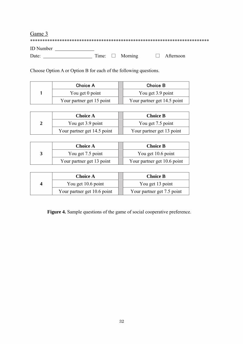
The third one is a game to extract social (cooperative) preferences. In this game, eight
pairs were made randomly. Each participant did not know who exactly her/his partner was.
Following Offerman (1996) and Park (2000), we used the method of value orientation,
which has been used not only in economics but also in other fields such as social psychology.
This game consisted of 24 questions, some of which are shown in Figure 4. For each
question, the participants had a choice between two alternatives: Choice A and Choice B.
Each option specified an amount of points to the participant ( x ) and an amount to the
partner ( y ). We set up the pairs of amounts of points so that 222 15 yx . Each participant
was told that her/his total points would be the sum of the amount s/he kept for her/himself
and the amount her/his partner gave to her/him. For example, in the case of Question 3, i) if
a participant chooses Choice A and her/his partner chooses Choice A, both s/he and her/his
partner receive 20.5 points, ii) if a participant chooses Choice A and her/his partner chooses
Choice B, s/he receives 18.1 points and her/his partner receives 23.6 points, iii) if s/he
chooses Choice B and her/his partner chooses Choice A, s/he receives 23.6 points and her/his
partner receives 18.1 points, and iv) if s/he chooses Choice B and her/his partner chooses
Choice B, both s/he and her/her partner receive 21.2 points.
We used each participant’s allocation of points to her/himself and her/his partner,
calculated the tangent/vector, and classified her/him into one of seven groups. In Figure 5,
the horizontal axis measures the total points of 24 questions for herself/himself, while the
vertical axis measures the total points of 24 questions for her/his partner. In general,
participants with observed vectors lying between degrees −112.5 and −67.5 are classified as
aggressive (or Type 1), participants with vectors between −67.5 and −22.5 are classified as
competitive (or Type 2), participants with vectors between −22.5 and 22.5 are classified as
individualistic (or Type 3), participants with vectors between 22.5 and 67.5 are classified as

14
cooperative (or Type 4), and participants with vectors between 67.5 and 112.5 are classified
as altruistic (or Type 5). We added 2 more categories: participants with observed vectors
lying between degrees −157.5 and −112.5 are classified as Type 0; participants with observed
vectors lying between degrees 112.5 and 157.5 are classified as Type 6. We used the number
of the type directly as an explanatory variable in Section 4. The larger this number is, the
more cooperative a participant is.
Figure 6 shows the distribution of participants in Games 1, 2, and 3. The distributions
seem to be ordinary ones. In Game 3, the numbers of types 3 and 4 are clearly larger than
those of other types. However, this type of distribution is usually observed with this value
orientation test.
3.2 Conjoint Questionnaire
After the experiment, we adopted the conjoint analysis method to extract the preferences of
Vietnamese consumers for secondhand products. We chose motorbikes and fridges as
products.
Most Vietnamese people own motorbikes. Even if a consumer does not own a motorbike
today, motorbikes are undeniably one of the important means to commute and, accordingly, a
motorbike is a realistic candidate of what s/he will purchase in the near future. Vietnamese
consumers are familiar with the prices, quality, and brands of motorbikes. In addition, lots of
dealers who sell secondhand motorbikes can be observed, and secondhand motorbikes are a
good option for consumers. Thus, we adopted motorbikes as one of the products for our
research. We also considered clarifying the relationship between environmental
consciousness and preference for secondhand products: whether a consumer cares about
saving electric bills may represent environmental consciousness. When we searched for the
electrical appliance stores in Hanoi in October 2014 in our pre-experimental survey, we saw

15
secondhand fridges. In addition, the Vietnamese government started a labeling scheme with
stars that represent the degree of energy saving, which is similar to energy stars.19 As of fall
in 2014, this label was attached to almost all of the new fridges in stores, and there is a
variety in the number of stars. Thus, we adopted fridges as the second product for our
research.
We choose five product attributes for motorbikes: price, product age, mileage, brand,
type, and origin. In general, price is definitely an important factor for consumers to
determine whether they will purchase a product. According to our pre-experimental survey,
the prices of new motorbikes ranged from VND 20 to 100 million, and the prices of new
motorbikes for the majority of consumers ranged from VND 30 to 50 million. Thus, we
adopted 10, 30, 50, and 70 million as the price levels for a conjoint analysis.20
Product age is the most important attribute for our purpose. A positive product age
(non-zero) implies that the product is secondhand. We adopted 0, 2, 4, 6 as product ages. We
also considered that instead of product age, mileage may play a key role when consumers
purchase motorbikes. Thus, we conducted another series of conjoint questions for mileages.
The following four levels are chosen: 0, 20,000, 40,000, and 60,000 kilometers.
Sometimes, brand is a key factor when buying a product. In particular, for older
Vietnamese people, Honda was a synonym for a motorbike. Whether a motorbike is a
scooter or an underbone is also an important factor. In particular, when a woman wears a
skirt, it is difficult for her to get on an underbone motorbike. Moreover, some consumers
believe that the quality of motorbikes made in Vietnam (or the production skill of domestic
workers) is lower than those from foreign (developed) countries. Thus, we also added the
place of production in the list of product attributes. We choose Honda and SYM as brands,
scooter and underbone as product types, and domestic and imported as origins. 19 The maximum number of stars is 5. 20 The price of 70 million may seem to be too high for secondhand motorbikes. However, some virtual motorbikes in the conjoint questions are new ones. Thus, we adopted these price levels.

16
We choose six product categories for fridges: price, product age, brand, size, the number of
energy stars, and origin. The reasons for choosing price, product age, brand, and origin are
similar to the case of motorbikes. We choose 4, 8, 15, and 25 million as price levels, 0, 2, 4,
and 6 as product ages. We also choose Hitachi and LG as brands, and domestic and imported
as origins.
In the case of motorbikes, consumers usually have a relatively small size of motorbike (125
cc displacement) in mind when they think of using one in their daily lives.21 This fact does
not depend on gender or age. Thus, we did not include the size of motorbikes as product
attributes. However, when it comes to fridges, the size or the number of doors matters. In the
pre-experimental survey, we asked a type of conjoint questions to consumers by designating
the number of doors. However, we found that the number of doors is sometimes confusing,
because there are big fridges with few doors and relatively small fridges with relatively
many doors. Thus, for accuracy, we adopted the sizes (litter) of fridges as a product attribute
and choose 140 and 450 litters as levels. Moreover, as noted above, the Vietnamese
government started a labeling scheme with stars that represent the degree of energy saving.
Thus, we also adopted the number of stars as a product attribute and choose 2 and 5 stars as
levels.
The product attributes and levels are summarized in Table 2.
We conducted three series of questions: motorbikes with product ages, motorbikes with
mileages, and fridges. For each series, we produced 16 virtual product profiles so that the
orthogonality condition is satisfied, and randomly made 8 pairs of profiles. We also chose
pairs for participants for each series. In each question, a participant had three choices: buy
either product or buy nothing. In total, each participant answered 24 questions. Examples of
conjoint questions are shown in Table 3.22
21 We explained about this point briefly before we began the conjoint survey. 22 We used the AlgDesign package of R to make these profiles satisfy the orthogonality condition.

17
3.3 Other Personal Attributes
Finally, participants were asked to answer questions about their personal attributes such as
age, gender, education, and so on. For the purpose of this research, we added several
important questions that are classified into two categories.
The questions in the first category relate to environmental consciousness. For the
analysis in Section 4, we made three variables. The first one is environmental consciousness
about general environmental problems. Participants were asked if they were interested in air
pollution, water/marine pollution, and global warming, and were given four choices for each
environmental problem: (i) I know about it, and am interested in it very much; (ii) I know
about it, but I am not very much interested in it; (iii) I do not know much about it, and I am
not interested in it; (iv) I have never heard about it. Almost all participants chose (i) or (ii).
Thus, we add one point when a participant chooses (i). Because there were three questions,
this variable ranged from zero to three. There were 23, 42, 72, and 147 participants with the
scores of 0, 1, 2, and 3, respectively.
The second variable is related to disposing behavior in which environmental
consciousness may be reflected. Participants were asked if they throw away garbage
anywhere other than the trash box when they are outside, and were given five choices:
always, often, sometimes, rarely, and never. We add 1, 2, 3, 4, and 5 points for always, often,
sometimes, rarely, and never, respectively. 14, 10, 35, 111, and 114 participants got 1, 2, 3, 4,
and 5 scores, respectively.
The third variable is related to contribution to environment through cost-saving activities.
Because the package chooses pairs randomly, we sometimes obtain meaningless pairs, which means that every respondent is expected to choose the same alternative. For example, consider the case in which the price of Product A is lower than Product B, and Product A is newer than Product B. Then, it is likely that every respondent will choose Product A than Product B. Only for the survey in June, 2015, we observed some obviously meaningless pairs. Therefore, we excluded those meaningless pairs.

18
Participants were asked if they care about saving electricity/water, and were given four
choices: very much, often, not very much, and not at all. Almost all participants chose very
much or often. Therefore, we added 1 point for very much, and 0 point for other choices. 101
participants were given 0 point, while 183 participants were given 1 point.
The questions in the second category are related to experience or knowledge. We made
three variables for this category. The first one is experience of selling used goods and wastes.
Participants were asked if they sell PET bottles, glass bottles, and cans (steel, aluminum,
etcetera) to junk buyers, and were given five choices: always, often, sometimes, rarely, and
never. We added 1, 2, 3, 4, and 5 points for never, rarely, sometimes, often, and always,
respectively. 10, 33, 113, 79, and 49 participants got 1, 2, 3, 4, and 5 scores, respectively.
The second variable is related to experience of owning secondhand motorbikes, which
can be used only for the analysis of preference for secondhand motorbikes. Of the
participants, 67 were owners of secondhand bikes, while 216 were owners of new bikes.23
The third variable is knowledge about labeling schemes of home appliances, which can
be used only for the analysis of preference for secondhand fridges. Participants were asked if
they knew about this labelling enforced in Vietnam. We added 1 point for participants who
knew this label, while 0 point for participants who did not know this label. 100 participants
did not know the label, while 99 participants had knowledge about the label before they
came to the survey. The number of participants who answered this question is 199, which
was much less than the total number of participants described above. In the sessions carried
out in January, we did not include this question in the questionnaire sheet. Thus, participants
who participated in the sessions carried out in May and June answered this question.
The details on the indices of variables used in the following analysis and expected signs
are described in Table 4.
23 The total number is 283 which is smaller than the number of participants. One participant did not answer this question.

19
4. Results
4.1 Estimation Method
We used multinomial logit to estimate the preference of consumers for motorbikes and
fridges.24 Basic multinomial models used for conjoint analyses assume that the condition of
independent of irrelevant alternatives (IIA condition) is satisfied. This condition requires that
the choice between certain two profiles/products is not influenced by any other
profiles/products. Because it is often indicated that IIA condition is difficult to satisfy, we
first conducted estimations of the effects of product attributes using both multinomial logit
model and random parameters logit models.25 We adopted normal and uniform distributions
for random parameters as possible approximations of the true coefficient distributions.26 We
used 100 Halton draws in the estimation of the random parameters logit models. First, we
assumed that the coefficients of all variables, except for the alternative specific constant
(ASC) and price, are randomly distributed. Second, we assumed that only the coefficients of
variables that obtained significant results in the first step are randomly distributed.
The results are shown in Tables 5(a), 5(b), and 5(c). In all cases, the results of the basic
multinomial logit model are almost the same as those of the random parameters logit models.
For almost all estimations, the coefficients of the standard deviation are not significant in the
second step. Thus, in the following analysis, we show the estimation results of the basic
multinomial logit models.27
24 We do not provide the basic description of multinomial logit estimation. For example, see Train (2009) for details among others. 25 For example, Hole and Kolstad (2012) estimated willingness-to-pay for health service jobs by using mixed logit estimation methods. 26 In fact, we also conducted lognormal distribution because this type of distribution is sometimes used in the literature. However, we obtained no significant results on the distributions. 27 The fact that the results are almost the same does not mean that there is no heterogeneity among consumers on the coefficients of product attributes. It is considered that normal and uniform distributions do not reflect the true coefficient distributions.

20
4.2 Results
Let us again focus on Tables 5(a), 5(b), and 5(c) to examine the basic results of only the
estimations with product attributes. For all three estimations, we obtained the expected signs
for all explanatory variables. The coefficient of price is significantly negative, which is
intuitive, because higher price is considered to affect consumer net surplus negatively. On
the other hand, the coefficients of other variables are significantly positive, which are also
intuitive or fit for real situations. As described in Table 4, the variable P-age/mileage is
larger as the age of a virtual product is younger, or as the mileage of a virtual product is
fewer. Thus, the positive coefficient of P-age/mileage implies that consumers prefer newer
products to older products. In Vietnam, Japanese brands are popular and, accordingly, the
coefficient of Honda/Hitachi is considered to be positive. Vietnamese consumers, in
particular, female consumers are likely to consider that scooters are stylish than underbone
motorbikes. The positive sign of the coefficient of scooter suggests this fact. Also, they
sometimes consider that the quality of motorbikes made in foreign (developed) countries is
higher than those made in Vietnam, which may lead to a positive sign for the coefficient of
import. The results on the size and number of stars for the estimation of demand for fridges
are also natural.
The negative result on alternative specific constants (ASC) is unexpected. This sign
implies that the number of consumers who chose to buy neither of the motorbikes lined up in
conjoint questions is not negligible. The possible reasons for this result are as follows. First,
the production of motorbikes has been increasing for the past few decades, and the import of
secondhand motorbikes has been banned, which implies that the supply of new motorbikes
has been increasing, while that of secondhand bikes has been relatively small. Then, the
price difference between new and secondhand motorbikes has become smaller. In addition,

21
the disposable income of the middle class has been increasing. Although we included new
motorbikes as one of the levels of product age/mileage, many choices were made between
two secondhand motorbikes. Thus, participants who have a strong preference for newness
might choose “Buy neither of the motorbikes.” The same situation holds for fridges. The
second possible reason is our price setting. Because new motorbikes can exist in profiles, we
set price levels so that VND 70 million is the maximum. However, 70 million (and possibly
50 million) may be too expensive for ordinary secondhand motorbikes.
Next, we examine the results of estimations with time, risk, and social cooperative
preferences, which are shown in Table 6. All possible cross terms of a product attribute and a
preference are taken into consideration. Several interesting results are obtained. First, the
coefficients of time-P-age/mileage are negative, and some of them are significant. This sign
implies that the more far-sighted a participant is, the stronger preference for aged or
secondhand products s/he has, which may seem to be counter intuitive. Far-sighted
consumers are likely to choose new products because they can be used for longer periods
compared to secondhand products. One interpretation is that far-sighted consumers care not
only about their own long-term surplus but also for the long-term social benefits. They may
consider that their society becomes more sustainable by using secondhand products.
Second, almost all of the coefficients of risk-P-age/mileage are negative, and some of
them are significant. This implies that the more risk-averting a participant is, the weaker
preference s/he has for secondhand products. This result is intuitive and consistent with the
theoretical result. Third, the coefficients of time-Honda/Hitachi are significantly positive.
Far-sighted consumers are likely to care more about the quality of products than
short-sighted consumers are. Thus, the positive coefficient implies that the former consumers
have an incentive to pay more for products of established brands. Fourth, the coefficients of
type-import are significantly negative. This result suggests that the more cooperative a
22
participant is, the less loyalty s/he feels for imported products. Fifth, the coefficient of
risk-star is significantly negative, which implies that the more risk averse a participant is, the
more seriously s/he cares about the labelling (the number of stars). This result is intuitive,
although the labelling may play the role of an index of high quality instead of conveying
information on cost saving.
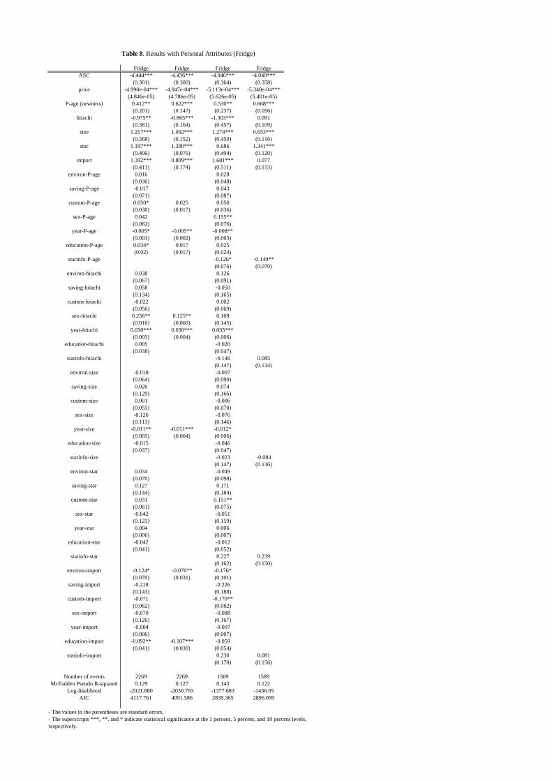
Finally, we examined the results of estimations with other personal attributes, which are
shown in Tables 7 and 8. All possible cross terms of a product attribute and a preference are
taken into consideration. Several interesting results are obtained.
There are five significant coefficients that are common to both motorbikes and fridges.
The coefficients of year-P-age are significantly negative. This result implies that the younger
a participant is, the weaker preference s/he has for secondhand products. In other words,
secondhand is not a serious negative factor for older consumers. The coefficients of
sex-Honda/Hitachi and year-Honda/Hitachi are positive, which is common to both
motorbikes and fridges. These results imply that male and/or older consumers are more
enthusiastic about Japanese brands than female and/or young consumers are. Moreover, the
coefficients of environ-import and education-import are negative. The results imply that the
more environmentally conscious a participant is, and the more educated a participant is, the
lower opinion s/he has of imported products. Environmentally conscious consumers may
care about the distance of transportation that may be directly proportional to environmental
pollution. Moreover, highly educated consumers are likely to take into consideration the true
quality of products. Thus, they may not think highly of foreign products only because they
are produced in foreign countries. Or, they may be less reluctant to purchase domestically
produced products because they are able to evaluate domestic products accurately.
Focusing on the results of the estimations of motorbikes, three additional significant
results are observed. The first two coefficients are related to gender difference. The

23
coefficients of sex-P-age and sex-import are significantly negative, which implies that male
consumers pay less attention to whether a product is new or secondhand and whether a
product is imported than female consumers are. The third coefficient is education-Honda,
which is significantly negative. The more highly educated a participant is, the less attention
s/he pays to the Honda brand. This result is consistent with the effect of education on the
enthusiasm for Japanese brands. Highly educated consumers may not think highly of Honda
motorbikes only because they are produced by Honda.
Focusing on the results of the estimations of fridges, two additional significant results are
observed. The coefficient of Starinfo-P-age is negative, which implies that a consumer who
is familiar with the labeling scheme before s/he came to the venue of the experimental
survey considers the age of the product less carefully than does a consumer who did not
know about the labeling scheme. If environmentally conscious consumers know the
existence of the labeling scheme better than environmentally unconscious consumers do, this
result also indicates that environmentally conscious consumers are more likely to prefer
secondhand products than environmentally unconscious consumers. The coefficient of
Custom-star is significantly positive, which implies that consumers who are familiar with the
secondhand markets care about the information of labeling. This result may also suggest that
labelling may play the role of an index of high quality.
One caveat should be noted. For some coefficients, the signs vary across estimation
equations depending on independent variables. This unstable result may arise because of
correlations among independent variables. However, we did not observe any strong
correlations among personal attributes. In addition, we focused only on the significant results.
Therefore, the results described in this subsection are considered to be the true.28
28 As noted in footnote 21, we excluded meaningless pairs in the survey carried out in June, 2015. This exclusion weakens the correlations among product attributes.

24
4.3. Discussion
Having looked at the results of the estimations, we now consider policy implications.
First, we focused on the behavior of far-sighted, environmentally conscious, and/or
highly educated consumers. What is common among these three types of consumers is that
they increase with economic development in general. From the review of the results, we saw
that far-sighted and/or environmentally conscious consumers have stronger preference for
secondhand products. And, environmentally conscious and highly educated consumers are
less enthusiastic about imported products compared to environmentally unconscious and low
educated consumers. In general, consumers classified into these three categories are easily
able to access information on quality and environmental aspects of products. Combining
these points, it can be said that the removal of import restrictions itself does not lead to
serious environmental pollution because the users of those secondhand products are likely to
care about the environmental aspects of products in the consumption stage.
Second, we focused on the strong preference for new products. As noted above, ASC is
negatively significant, which suggests the possibility that ordinary Vietnamese consumers
basically think about purchasing new products. And, younger consumers are verified to be
more enthusiastic about newness than older consumers are. Combining these results with the
results on the coefficients relating to origin/import, even if trade in secondhand products is
liberalized, domestically produced new motorbikes will not lose market share. It is likely
that new and secondhand products are well-differentiated.
Third, we investigated the importance of the labeling scheme on secondhand products.
As noted in the previous subsection, the results of the coefficients relating to the labeling
scheme on fridges/home appliances suggest that consumers consider labeling as an index of
high quality. However, this type of labeling should also convey information on
environmental and health problems. In general, prices are unlikely to reflect the

25
environmental values of products, because environmental values include external benefits. It
is also unlikely that prices reflect the value of good health because of the asymmetric
information between producers and consumers. Introduction of information transmission
systems through the markets mitigates the degree of the problem.
According to the result of the coefficient on risk preference, risk averters do not like
secondhand products. One important reason for this situation is that Vietnamese consumers
do not trust the quality of secondhand products. Thus, it is important to introduce reliable
labeling or information transmission schemes on secondhand products. Introduction of these
schemes enhances the value of branded secondhand products, because labeling can play a
role in guaranteeing quality. It is also important for this type of labeling to convey
environmental information. Then, an increase in imports of secondhand products is not
directly connected to serious environmental pollution. Consequently, trade liberalization of
secondhand products consorts with environmental protection.
5. Conclusion
In this paper, we delved into the demand side of secondhand products by using field
experimental data carried out in the northern part of Vietnam. In particular, we examined if
the demand for secondhand products is large in Vietnam, what types of consumers have
stronger preference for secondhand goods, and if imports of secondhand goods are directly
connected to environmental and health problems.
We obtained a set of interesting results on (i) the relationship between product attributes
and demand and (ii) the relationship between product and personal attributes. Those results
provide important policy implication on trade and the environmental aspects of secondhand
products. Although it is possible that the situation on preference for secondhand products
varies across countries, we believe that the importance of investigating the issue of

26
secondhand products in terms of both demand and supply is verified.
Reference
Amador, F. J., R M. González and F. J. Ramos-Real (2013). Supplier choice and WTP for
electricity attributes in an emerging market: The role of perceived past experience,
environmental concern and energy saving behavior. Energy Economics 40, 953-966.
Anderson, S. P. and V. A. Ginsburgh (1994). Price discrimination via second-hand markets.
European Economic Review 38, 23-44.
Banfi, S., M. Filipini and A. Horehájová (2012). Using a choice experiment to estimate the
benefits of a reduction of externalities in urban areas with special focus on electrosmog,
Applied Economics 44, 387-397.
Bond, E. W. and T Iizuka (2014). Durable goods price cycles: theory and evidence from the
textbook market, Economic Inquiry 52, 518-538.
Clerides, S. (2008). Gains from trade in used goods: Evidence from automobiles. Journal of
International Economics 76, 322-336.
Clerides, S. and C. Hadjiyiannis (2008). Quality standards for used durables: An indirect
subsidy? Journal of International Economics 75, 268-282.
Disdier, A. and S. Marette (2013). Globalization issues and consumers’ purchase decisions
for food products: evidence from a laboratory experiment, European Review of
Agricultural Economics 40, 23-44.
Fudenberg, D. and J. Tirole (1998). Upgrades, tradeins, and buybacks, RAND Journal of
Economics 29, 235-258.
Hole, A. R. and J. R. Kolstad (2012). Mixed logit estimation of willingness to pay
distributions: A comparison of models in preference and WTP space using data from a
health-related choice experiment, Empirical Economics 42, 445-469.

27
Jin, J., Z. Wang and S. Ran (2006). Comparison of contingent valuation and choice
experiment in solid waste management programs in Macao, Ecological Economics 57,
430-441.
Keisaku, H. and S. Managi (2014). Determinants of trade in recyclable wastes: Evidence
from commodity-based trade of waste and scrap, Environment and Development
Economics 19, 250-270.
Kellenberg, D. (2010). Consumer waste, backhauling, and pollution havens. Journal of
Applied Economics 13, 283-304.
Kinnaman, T. and H. Yokoo (2011). The environmental consequences of global reuse.
American Economic Review 101, 71-76.
Kumar, P. (2002). Price and quality discrimination in durable goods monopoly with resale
trading, International Journal of Industrial Organization 20, 1313-1339.
Offerman, J. S., and A. Schram (19969. Value orientations, expectations and voluntary
contributions in public goods, Economic Journal 106, 817-854.
Park, E. (2000). Warm-glow versus cold-prickle: a further experimental study of framing
effects on free-riding, Journal of Economic Behavior and Organization 43, 405-421.
Ray, A. (2008). Waste management in developing Asia: can trade and cooperation help?
Journal of Environment and Development 17, 3-25.
Shinkuma, T., and N. T. M. Huong (2009). The flow of E-waste material in the Asian region
and a reconsideration of international trade policies on E- waste. Environmental Impact
Assessment Review 29, 25-31.
Tarfasa, S. and R. Brouwer (2013). Estimation of the public benefits of urban water supply
improvements in Ethiopia: A choice experiment, Applied Economics 45, 1099-1108.
Train, K. E. (2009). Discrete choice methods with simulation, 2nd edn. Cambridge
University Press, Cambridge.

28
Van Beukering, P. J. H. and M. N. Bouman (2001). Empirical evidence on recycling and
trade of paper and lead in developed and developing countries, World Development 29,
1717-1737.
Voors, M. J., E. E. M. Nillesen, P. Verwimp, E. H. Bulte, R. Lensink and D. P. Van Soest
(2012). Violent conflict and behavior: A field experiment in Burundi, American Economic
Review 102, 941-964.
Wong, M. H., S. C. Wu, W. J. Deng, X. Z. Yu, Q. Luo, A. O. W. Leung, and C. S. C. Wong,
W. J. Luksemburg, and A. S. Wong (2007). Export of toxic chemicals ? A review of the
case of uncontrolled electronic-waste recycling. Environmental Pollution 149, 131-140.

29
Figure 1. Japan's export amount of secondhand vehicles. Source: Trade statistics, the Japan Customs
0
200
400
600
800
1000
120020
01
2002
2003
2004
2005
2006
2007
2008
2009
2010
2011
2012
2013
2014
Number (thousand)
Value (billion JPY)

30
Game 1 *************************************************************************
ID Number
Date: Time: □ Morning □ Afternoon
Choose Option A or Option B for each of the following questions.
Figure 2. Questions of the game of risk preference
1
Choice A
Payoff
VND 60,000 + VND 15,000
Choice B
Color of the ball Payoff
●●● VND 60,000 + VND 60,000
○○○○○○○ VND 60,000 + VND 0
2
Choice A
Payoff
VND 60,000 + VND 18,000
Choice B
Color of the ball Payoff
●●● VND 60,000 + VND 60,000
○○○○○○○ VND 60,000 + VND 0
3
Choice A
Payoff
VND 60,000 + VND 21,000
Choice B
Color of the ball Payoff
●●● VND 60,000 + VND 60,000
○○○○○○○ VND 60,000 + VND 0
4
Choice A
Payoff
VND 60,000 - VND 15,000
Choice B
Color of the ball Payoff
●●● VND 60,000 - VND 60,000
○○○○○○○ VND 60,000 - VND 0
5
Choice A
Payoff
VND 60,000 - VND 18,000
Choice B
Color of the ball Payoff
●●● VND 60,000 - VND 60,000
○○○○○○○ VND 60,000 - VND 0
6
Choice A
Payoff
VND 60,000 - VND 21,000
Choice B
Color of the ball Payoff
●●● VND 60,000 - VND 60,000
○○○○○○○ VND 60,000 - VND 0

31
Figure 3. Questions of the game of the time preference.
A B
Receive VND 40,000 today Receive VND 40,000 two weeks from now
A B
Receive VND 40,000 today Receive VND 40,400 two weeks from now
A B
Receive VND 40,000 today Receive VND 40,800 two weeks from now
A B
Receive VND 40,000 today Receive VND 42,000 two weeks from now
A B
Receive VND 40,000 today Receive VND 44,000 two weeks from now
A B
Receive VND 40,000 today Receive VND 56,000 two weeks from now
A B
Receive VND 40,000 today Receive VND 68,000 two weeksfrom now
A B
Receive VND 40,000 today Receive VND 80,000 two weeks from now
7
8
1
2
3
4
5
6
32
Game 3 *************************************************************************
ID Number
Date: Time: □ Morning □ Afternoon
Choose Option A or Option B for each of the following questions.
1
Choice A Choice B
You get 0 point You get 3.9 point
Your partner get 15 point Your partner get 14.5 point
2
Choice A Choice B
You get 3.9 point You get 7.5 point
Your partner get 14.5 point Your partner get 13 point
3
Choice A Choice B
You get 7.5 point You get 10.6 point
Your partner get 13 point Your partner get 10.6 point
4
Choice A Choice B
You get 10.6 point You get 13 point
Your partner get 10.6 point Your partner get 7.5 point
Figure 4. Sample questions of the game of social cooperative preference.

33
Figure 5. Allocation of points and type classification.
*Horizontal axis measures the total points for herself/himself, while
vertical axis measures the total points for her/his partner.
4
3
2
1
0
5
6

34
Figure 6. Distribution of subjects in games 1, 2, and 3.
*In Games 1 and 2, the horizontal axis is the number of choosing Choice B.
In Game 3, the horizontal axis is type.
0
20
40
60
80
100
120
140
160
0 1 2 3 4 5 6
Game 1 - risk preference -
0
10
20
30
40
50
60
70
0 1 2 3 4 5 6 7 8
Game 2 - time preference -
0
20
40
60
80
100
120
140
160
0 1 2 3 4 5 6
Game 3 -social cooperative preference -

Dates City Venue Number of Sessions Number of Subjects
January 9, 10, 11, 2015 Hanoi Hanoi Foreign TradeUniversity 5 17, 15, 18, 21, 14
May 9, 10, 11, 2015 Hanoi NIIT-ICT Hanoi 5 11, 19, 15, 20, 16, 18
June 6, 2015 Thai Ping Le Hong Phong SecondarySchool 2 18, 18
June 7, 8, 2015 Thai Hong Thai Hong Commune People'sCommittee Meeting Hall 4 17, 16, 15, 16
Table 1. Details of Survey

MotorbikeProduct Attribute Level 1 Level 2 Level 3 Level 4Price (1 million) 10 30 50 70
Prouct age(Mileage km) 0 (0) 2 (20000) 4 (40000) 6 (60000)
Brand Honda SYMType Scooter Underbone
Origin Imported Domestic
FridgeProduct Attribute Level 1 Level 2 Level 3 Level 4Price (1 million) 4 8 15 25
Product age 0 2 4 6Brand Hitachi LG
Size (litter) 140 450Energy star ☆☆☆☆☆ ☆☆
Origin Imported Domestic
Table 2. Product Attributes and Levels

Motorbike A Motorbike BQ1 Price 30 Price 10
Product age 0 Product Age 6Brand Honda Brand SYMType Underbone Type Scooter
Origin Domestic Origin Domestic
Motorbike A Motorbike BQ1 Price 30 Price 30
Mileage 40,000 Mileage 20,000Brand Honda Brand SYMType Underbone Type Scooter
Origin Domestic Origin Imported
Fridge A Fridge BQ1 Price 800 Price 1,500
Product age 0 Product age 2Brand LG Brand HitachiSize 140 Size 450
Energy star ☆☆ Energy star ☆☆☆☆☆Origin Imported Origin Domestic
1. Buy motorbike A2. Buy motorbike B3. Do not want to buy either A or B
1. Buy motorbike A2. Buy motorbike B3. Do not want to buy either A or B
1. Buy fridge A2. Buy fridge B3. Do not want to buy either A or B
Table 3. Sample questions
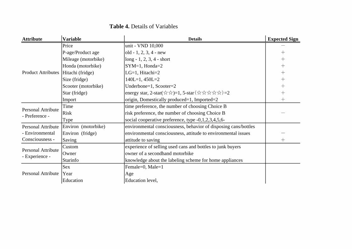
Attribute Variable Details Expected SignPrice unit - VND 10,000 -
P-age/Product age old - 1, 2, 3, 4 - new +
Mileage (motorbike) long - 1, 2, 3, 4 - short +
Honda (motorbike) SYM=1, Honda=2 +
Hitachi (fridge) LG=1, Hitachi=2 +
Size (fridge) 140L=1, 450L=2 +
Scooter (motorbike) Underbone=1, Scooter=2 +
Star (fridge) energy star, 2-star(☆☆)=1, 5-star(☆☆☆☆☆)=2 +
Import origin, Domestically produced=1, Imported=2 +
Time time preference, the number of choosing Choice BRisk risk preference, the number of choosing Choice B -
Type social cooperative preference, type -0,1,2,3,4,5,6-Environ (motorbike) environmental consciousness, behavior of disposing cans/bottlesEnviron (fridge) environmental consciousness, attitude to environmental issues -
Saving attitude to saving +
Custom experience of selling used cans and bottles to junk buyersOwner owner of a secondhand motorbikeStarinfo knowledge about the labeling scheme for home appliancesSex Female=0, Male=1Year AgeEducation Education level,
Personal Attribute
Table 4. Details of Variables
Product Attributes
Personal Attribute- Preference -
Personal Attribute- EnvironmentalConsciousness -
Personal Attribute- Experience -

Bike-Age Bike-Age Bike-Age Bike-Age Bike-AgeASC -2.982*** -3.022*** -2.994*** -3.036*** -2.981***
(0.209) (0.218) (0.211) (0.222) (0.210)price -1.176e-04*** -1.208e-04*** -1.181e-04*** -1.225e-04*** -1.170e-04***
(1.506e-05) (1.592e-05) (1.536e-05) (1.633e-05) (1.538e-05)product age (P-age, newness) 0.584*** 0.608*** 0.589*** 0.624*** 0.580***
(0.032) (0.039) (0.035) (0.043) (0.035)honda 0.783*** 0.827*** 0.790*** 0.848*** 0.778***
(0.066) (0.073) (0.068) (0.077) (0.068)scooter 0.194*** 0.186*** 0.194*** 0.165*** 0.198***
(0.067) (0.067) (0.064) (0.073) (0.067)import 0.340*** 0.341*** 0.340*** 0.351*** 0.337***
(0.070) (0.073) (0.069) (0.075) (0.070)SD age -0.014 -0.010
(0.168) (0.300)SD honda 0.097 0.189
(0.270) (0.484)SD scooter 0.101 0.618** -0.348
(0.272) (0.300) (0.351)SD import 0.410** 0.189 0.690** 0.014
(0.163) (0.216) (0.282) (0.489)
Distribution Normal Normal Uniform UniformNumber of Events 2272 2272 2272 2272 2272
Log-likelihood -2188.6 -2187.3 -2188.4 -2186.9 -2187.4AIC 4389.188 4394.695 4390.766 4393.844 4390.849
- The values in the parentheses are standard errors.- The superscripts ***, **, and * indicate statistical significance at the 1 percent, 5 percent, and 10 percent levels,respectively.
Table 5(a): Basic Results on Product Attributes (Moterbike with Age)

Bike-Mileage Bike-Mileage Bike-MileageASC -3.137*** -3.177*** -3.176***
(0.217) (0.222) (0.222)price -1.355e-04*** -1.400e-04*** -1.398e-04***
(1.534e-05) (1.539e-05) (1.536e-05)mileage (newness) 0.550*** 0.578*** 0.575***
(0.032) (0.038) (0.038)honda 0.950*** 0.991*** 0.991***
(0.074) (0.083) (0.083)scooter 0.268*** 0.267*** 0.268***
(0.069) (0.073) (0.073)import 0.380*** 0.375*** 0.375***
(0.067) (0.073) (0.073)SD mileage -0.042 -0.081
(0.158) (0.272)SD honda 0.213 0.340
(0.227) (0.406)SD scooter 0.142 0.249
(0.252) (0.432)SD import 0.308 0.523
(0.202) (0.337)
Distribution Normal UniformNumber of Events 2182 2182 2182
Log-likelihood -2110.8 -2108.6 -2108.9AIC 4233.665 4237.272 4237.728
Table 5(b): Basic Results on Product Attributes (Moterbike with Mileage)
- The values in the parentheses are standard errors.- The superscripts ***, **, and * indicate statistical significance at the 1 percent, 5percent, and 10 percent levels, respectively.

Fridge Fridge Fridge Fridge FridgeASC -4.450*** -4.586*** -4.476*** -4.601*** -4.453***
(0.297) (0.325) (0.308) (0.325) (0.301)price -5.254e-04*** -5.867e-04*** -5.333e-04*** -5.904e-04*** -5.265e-04***
(4.697e-05) (5.172e-05) (4.810e-05) (5.193e-05) (4.621e-05)product age (P-age, newness) 0.600*** 0.645*** 0.609*** 0.648*** 0.602***
(0.036) (0.042) (0.038) (0.042) (0.036)hitachi 0.225*** 0.255*** 0.227*** 0.259*** 0.225***
(0.069) (0.081) (0.073) (0.081) (0.071)size 0.732*** 0.803*** 0.743*** 0.810*** 0.734***
(0.075) (0.086) (0.080) (0.086) (0.077)star 1.390*** 1.514*** 1.407*** 1.530*** 1.392***
(0.076) (0.086) (0.084) (0.099) (0.079)import 0.138** 0.131* 0.139* 0.129 0.138**
(0.068) (0.078) (0.072) (0.079) (0.070)SD age 0.001 0.011
(0.182) (0.311)SD hitachi 0.285 0.462
(0.254) (0.447)SD size 0.000 0.071
(0.320) (0.547)SD star 0.689*** 0.362** 1.207*** 0.190
(0.141) (0.153) (0.217) (0.417)SD import 0.091 0.203
(0.296) (0.499)
Distribution Normal Normal Uniform UniformNumber of Events 2269 2269 2269 2269 2269
Log-likelihood -2077.6 -2068.6 -2075.4 -2067.5 -2077.5AIC 4169.109 4161.265 4166.857 4158.900 4170.996
- The values in the parentheses are standard errors.- The superscripts ***, **, and * indicate statistical significance at the 1 percent, 5 percent, and 10 percent levels,respectively
Table 5(c): Basic Results on Product Attributes (Fridge)

Bike-Age Bike-Age Bike-Age Bike-Mileage Bike-Mileage Bike-Mileage Fridge Fridge FridgeASC -2.985*** -2.986*** -3.000*** -3.140*** -3.134*** -3.137*** -4.450*** -4.453*** -4.452***
(0.210) (0.210) (0.211) (0.218) (0.218) (0.218) (0.296) (0.297) (0.297)price -1.118e-04*** -1.184e-04*** -1.186e-04*** -1.355e-04*** -1.370e-04*** -1.371e-04*** -5.291e-04*** -5.275e-04*** -5.299e-04***
(1.508e-05) (1.511e-05) (1.515e-05) (1.535e-05) (1.539e-05) (1.541e-05) (4.706e-05) (4.704e-05) (4.725e-05)P-age/mileage (newness) 0.751*** 0.709*** 0.640*** 0.709*** 0.635*** 0.603*** 0.689*** 0.716*** 0.501***
(0.072) (0.107) (0.122) (0.073) (0.100) (0.114) (0.075) (0.106) (0.122)honda/hitachi 0.784*** 0.886*** 0.807*** 0.953*** 1.151*** 1.039*** 0.227*** 0.169 -0.302
(0.066) (0.190) (0.228) (0.075) (0.191) (0.249) (0.069) (0.190) (0.235)size 0.734*** 0.734*** 0.395*
(0.075) (0.075) (0.233)scooter 0.195*** 0.193*** -0.248 0.266*** 0.268*** 0.170
(0.067) (0.067) (0.242) (0.069) (0.069) (0.254)star 1.390*** 1.390*** 1.890***
(0.076) (0.076) (0.264)import 0.340*** 0.341*** 1.021*** 0.382*** 0.380*** 0.666*** 0.139** 0.138** 0.891***
(0.070) (0.070) (0.256) (0.067) (0.067) (0.233) (0.068) (0.069) (0.266)time-P-age/mileage -0.002 -0.025** -0.034*** -0.005 -0.015 -0.016 0.003 -0.013 -0.008
(0.007) (0.011) (0.012) (0.007) (0.018) (0.012) (0.007) (0.011) (0.013)risk-P-age/mileage -0.041*** -0.043* -0.030 -0.016 -0.008 0.002 -0.023 -0.020 0.007
(0.014) (0.022) (0.026) (0.014) (0.021) (0.024) (0.014) (0.022) (0.026)type-P-age/mileage -0.010 0.021 0.037 -0.026** -0.005 -0.003 -0.009 -0.005 0.028
(0.013) (0.020) (0.023) (0.013) (0.018) (0.021) (0.013) (0.019) (0.023)time-honda/hitachi 0.052*** 0.029 0.025 0.020 0.039** 0.051**
(0.019) (0.023) (0.020) (0.026) (0.019) (0.024)risk-honda/hitachi 0.006 0.021 -0.021 0.010 -0.006 0.050
(0.040) (0.048) (0.039) (0.053) (0.039) (0.050)type-honda/hitachi -0.072** -0.044 -0.057* -0.047 -0.010 0.064
(0.035) (0.042) (0.034) (0.045) (0.034) (0.044)time-size 0.003
(0.023)risk-size 0.067
(0.048)type-size 0.033
(0.044)time-scooter 0.041 0.013
(0.025) (0.027)risk-scooter 0.062 0.008
(0.052) (0.054)type-scooter 0.037 0.011
(0.044) (0.047)time-star -0.034
(0.026)risk-star -0.130**
(0.055)type-star -0.003
(0.048)time-import 0.003 -0.006 0.009
(0.026) (0.025) (0.027)risk-import -0.010* -0.061 -0.048
(0.054) (0.048) (0.054)type-import -0.103** -0.025 -0.172***
(0.048) (0.044) (0.052)
Number of Events 2272 2272 2272 2182 2182 2182 2269 2269 2269McFadden Pseudo R-squared 0.088 0.089 0.091 0.085 0.085 0.086 0.115 0.116 0.119
Log-likelhood -2183.505 -2176.977 -2170.692 -2107.766 -2105.224 -2104.082 -2075.927 -2073.722 -2061.827AIC 4385.01 4377.954 4377.385 4233.533 4234.447 4244.163 4171.854 4173.444 4167.655
- The values in the parentheses are standard errors.- The superscripts ***, **, and * indicate statistical significance at the 1 percent, 5 percent, and 10 percent levels, respectively.
Table 6. Results with Risk, Time, and Social Cooperative Preferences

Bike-Age Bike-Age Bike-Mileage Bike-MileageASC -3.050*** -3.028*** -3.155*** -3.172***
(0.215) (0.214) (0.022) (0.219)price -1.183e-04*** -1.172e-04*** -1.458e-04*** -1.433e-04***
(1.540e-05) (1.530e-05) (1.556e-05) (1.540e-05)P-age/mileage (newness) 0.829*** 0.980*** 0.655*** 0.770***
(0.214) (0.086) (0.197) (0.081)honda 0.261 0.339** 1.048** 1.201***
(0.399) (0.168) (0.440) (0.180)scooter -0.591 -0.463*** 0.460 0.278***
(0.438) (0.168) (0.457) (0.070)import 1.395*** 1.138*** 0.649 0.395***
(0.449) (0.173) (0.412) (0.068)environ-P-age 0.026 -0.012 -0.045***
(0.028) (0.026) (0.017)owner-P-age 0.028 0.063 0.133***
(0.070) (0.066) (0.041)custom-P-age 0.004 0.015
(0.029) (0.027)sex-P-age -0.008 -0.047 -0.119**
(0.061) (0.056) (0.048)year-P-age -0.011*** -0.011*** -0.003
(0.003) (0.002) (0.003)education-P-age 0.006 0.006
(0.020) (0.018)environ-honda -0.040 -0.006
(0.050) (0.055)owner-honda 0.072 0.168
(0.128) (0.145)custom-honda 0.019 -0.002
(0.053) (0.058)sex-honda 0.336*** 0.250*** 0.317** 0.193**
(0.112) (0.094) (0.124) (0.090)year-honda 0.011** 0.011** 0.007 0.006**
(0.005) (0.004) (0.005) (0.003)education-honda 0.026 -0.102** -0.112***
(0.036) (0.040) (0.021)environ-scooter 0.071 -0.038
(0.056) (0.060)owner-scooter -0.035 -0.101
(0.143) (0.152)custom-scooter -0.028 -0.019
(0.058) (0.061)sex-scooter -0.184 -0.102
(0.124) (0.130)year-scooter 0.018*** 0.018*** 0.000
(0.005) (0.004) (0.006)education-scooter 0.009 0.022
(0.040) (0.042)environ-import -0.117** -0.054* -0.032
(0.060) (0.030) (0.060)owner-import 0.096 0.125
(0.144) (0.138)custom-import 0.018 -0.006)
(0.060) (0.058)sex-import -0.256** -0.348*** -0.175
(0.126) (0.100) (0.120)year-import 0.001 0.004
(0.005) (0.005)education-import -0.121*** -0.087*** -0.042
(0.040) (0.019) (0.038)
Number of events 2272 2272 2182 2182McFadden Pseudo R-squared 0.102 0.099 0.096 0.094
Log-likelihood -2131.114 -2139.337 -2066.886 -2073.95AIC 4322.228 4304.673 4193.771 4171.901
Table 7. Results with Personal Attributes
- The values in the parentheses are standard errors.- The superscripts ***, **, and * indicate statistical significance at the 1 percent, 5 percent, and 10percent levels, respectively.
Fridge Fridge Fridge FridgeASC -4.444*** -4.436*** -4.046*** -4.040***
(0.301) (0.300) (0.364) (0.358)price -4.990e-04*** -4.947e-04*** -5.113e-04*** -5.340e-04***
(4.846e-05) (4.786e-05) (5.626e-05) (5.401e-05)P-age (newness) 0.412** 0.622*** 0.530** 0.668***
(0.201) (0.147) (0.237) (0.056)hitachi -0.975** -0.865*** -1.303*** 0.091
(0.381) (0.164) (0.457) (0.109)size 1.257*** 1.092*** 1.274*** 0.653***
(0.368) (0.152) (0.450) (0.116)star 1.197*** 1.390*** 0.686 1.341***
(0.406) (0.076) (0.494) (0.120)import 1.392*** 0.809*** 1.681*** 0.077
(0.411) (0.174) (0.511) (0.113)environ-P-age 0.016 0.028
(0.036) (0.048)saving-P-age -0.017 0.043
(0.071) (0.087)custom-P-age 0.050* 0.025 0.050
(0.030) (0.017) (0.036)sex-P-age 0.042 0.155**
(0.062) (0.076)year-P-age -0.005* -0.005** -0.008**
(0.003) (0.002) (0.003)education-P-age 0.034* 0.017 0.025
(0.02) (0.017) (0.024)starinfo-P-age -0.126* -0.149**
(0.076) (0.070)environ-hitachi 0.038 0.126
(0.067) (0.091)saving-hitachi 0.058 -0.050
(0.134) (0.165)custom-hitachi -0.022 0.002
(0.056) (0.069)sex-hitachi 0.256** 0.125** 0.169
(0.016) (0.060) (0.145)year-hitachi 0.030*** 0.030*** 0.035***
(0.005) (0.004) (0.006)education-hitachi 0.005 -0.020
(0.038) (0.047)starinfo-hitachi -0.146 0.085
(0.147) (0.134)environ-size -0.018 -0.007
(0.064) (0.090)saving-size 0.026 0.074
(0.129) (0.166)custom-size 0.001 -0.006
(0.055) (0.070)sex-size -0.126 -0.076
(0.113) (0.146)year-size -0.011** -0.011*** -0.012*
(0.005) (0.004) (0.006)education-size -0.015 -0.046
(0.037) (0.047)starinfo-size -0.023 -0.084
(0.147) (0.136)environ-star 0.034 -0.049
(0.070) (0.098)saving-star 0.127 0.171
(0.144) (0.184)custom-star 0.031 0.151**
(0.061) (0.075)sex-star -0.042 -0.051
(0.125) (0.159)year-star 0.004 0.006
(0.006) (0.007)education-star -0.042 -0.012
(0.041) (0.052)starinfo-star 0.227 0.239
(0.162) (0.150)environ-import -0.124* -0.076** -0.176*
(0.070) (0.031) (0.101)saving-import -0.218 -0.226
(0.143) (0.188)custom-import -0.071 -0.170**
(0.062) (0.082)sex-import -0.070 -0.088
(0.126) (0.167)year-import -0.004 -0.007
(0.006) (0.007)education-import -0.092** -0.107*** -0.059
(0.041) (0.030) (0.054)starinfo-import 0.230 0.081
(0.170) (0.156)
Number of events 2269 2269 1589 1589McFadden Pseudo R-squared 0.129 0.127 0.143 0.122
Log-likelihood -2021.880 -2030.793 -1377.683 -1436.05AIC 4117.761 4091.586 2839.365 2896.099
- The values in the parentheses are standard errors.- The superscripts ***, **, and * indicate statistical significance at the 1 percent, 5 percent, and 10 percent levels,respectively.
Table 8. Results with Personal Attributes (Fridge)