Are Durable Goods Consumers Forward Looking?

Evidence from College Textbooks

Judith A Chevalier Yale School of Management and NBER

Austan Goolsbee

University of Chicago Graduate School of Business and NBER

Draft: December 2005

Abstract: Popular wisdom holds that publishers revise college textbooks mainly to kill off the secondary market for used books. While this behavior might be profitable if consumers are myopic, uninformed or have high short-run discount rates (that exceed the publishers'), neoclassical authors have noted that it will typically not be profitable if publishers can precommit not to cut prices and if consumers are forward-looking and have similar discount rates as the publishers; the consumer's willingness to pay for new books falls if they know that they cannot resell their used books. Using a large new dataset on all textbooks sold in psychology, biology and economics in the 10 semesters from 1997 to 2001, we estimate a demand system for books to test whether textbook consumers are forward-looking. The data strongly support the view that students are forward-looking with low short-run discount rates and that they have rational expectations of publishers' revision behavior. When the students buy their textbooks, they correctly take into account the probability that they will not be able to resell their books at the end of the semester due to a new edition release. Conditional on faculty assignment behavior, simulation results suggest that students are sufficiently forward looking that publishers could not raise revenues by accelerating current revision cycles. __________________ The authors wish to thank Pat Bajari, Steven Berry, Keith Chen, Ken Hendricks, Sharon Oster, Alan Sorensen, Jesse Shapiro, and especially J.P. Dube for helpful comments and assistance with the paper as well as seminar participants at Columbia, Duke, Harvard Business School, the NBER IO meetings, Princeton, the Quantitative Marketing and Economics conference, Yale, the University of Chicago and U.S.C. . Goolsbee wishes to thank the National Science Foundation (SES-0312749) for financial support.

2

The pricing and design of durable goods has been the focus of an enormous literature in economics. Frequently, however, theoretical results contradict popularly-held views of durable goods markets. For example, many basic theories and conventional wisdom greatly diverge on the question of whether producers have an incentive to eliminate resale markets for their used products. Conventional wisdom suggests that the existence of resale markets is bad for producers and that producers have an incentive to kill off resale markets. For example, in 2002, the Authors Guild, a trade group for writers, called upon its members to boycott Amazon.com for launching a market in used books.

However, a basic neoclassical model of durable goods markets suggests that a monopoly producer who can pre-commit to future prices should not feel threatened by the opening of resale markets. This is because rational forward-looking consumers will fully incorporate expectations about future resale opportunities into their willingness to pay for a good today. 1 Rational, forward-looking consumers are also crucial for the important literature extending the conventional analysis to models that address time-consistency issues on the part of the producer. 2

Recent work in behavioral economics, however, has attacked that view of consumers. Two strands of the behavioral literature are especially relevant. First, behavioral economics has argued that individuals are myopic; they have a difficult time evaluating future payoffs relative to current payoffs.3 Second, even when consumers fully comprehend future payoffs, a large behavioral literature argues that they tend to have extremely high short-run discount rates.4 If consumers are not fully forward-looking, or if they have exceedingly high short run discount rates, their willingness to pay for a good may not respond much to the future resale price of the good. If consumers fail to forecast the future or discount future payments at a much higher rate than do producers, producers may find it optimal to charge lower prices for their new goods and then undertake actions to kill the resale markets for used goods.5 That is, the opportunity for a producer to lower the resale value of the good ex post may be a “shrouded attribute” of a good, as in Gabaix and Laibson (2005). The publishers can exploit the ignorance or impatience of the consumers.

The market for textbooks provides a “textbook case” of the divergence between the neoclassical and the popular/behavioral views regarding durable goods. Publishers

1 Indeed, some authors raised precisely the neoclassical arguments in opposing the Author’s Guild Boycott of Amazon. See Nasar (2002). This argument is put forward in Friedman (1961), Miller (1974) and Swan (1970,1971), among others. 2 See, for example, Coase (1972), Swan (1980), Stokey (1981), Bulow (1982), Bulow (1986), Gul et. al. (1986), Carlton and Gertner (1989), and Waldman (1993). 3 McClure et. al. (2004), for example, present brain scan evidence illustrating that evaluating the future involves is more cognitively costly than evaluating the present. 4 Frederick et al. (2002) provide an overview of the voluminous behavioral literature on time discounting and time preference. 5 Barro (1972) and Nocke and Pietz (2002), for example, establish such results in durable goods models.

3

revise textbooks frequently and when they do, college bookstores almost immediately stop selling older editions. The popular view holds that publishers exploit students by introducing these new editions because they are trying simply to eliminate competition from inexpensive used books.6 Traditional economic reasoning, as described in Friedman (1962), Miller (1974), or Swan (1970,1971) claims that this argument does not make sense; forward-looking consumers will pay less for new books if they cannot sell them back at the end of the year.7 Indeed, under some basic assumptions about the market, one can show that publisher revenues should be invariant to the expected life of a college textbook. In such a model, revisions must be driven by some other factor such as demand for updated content.8 In this paper, we use a new dataset of college textbook assignments and college textbook purchases (new and used) in the disciplines of economics, psychology, and biology to study how forward-looking the buyers of college textbooks are and the implications of their behavior for publishers. Despite its status as a classic example of a durable good, the textbook industry has seldom been studied empirically. 9 We start by noting the many ways that the textbook market provides an ideal empirical setting to examine forward-looking behavior because it lacks many of the complicating factors found in other such industries. Then, we establish three basic results. First, we show that the prices of new and used books remain fairly constant over the life of an edition, while the probability that the edition is revised (thus rendering the book unable to be resold to the campus bookstore) varies rather dramatically over the life of the edition and across fields. This means that the purchasing behavior of an elastic forward-looking consumer (i.e., one that takes into account the ability to resell the book at the end of the semester) should change over the life of the edition in a way that the behavior of a myopic consumer or a consumer with a high short-run discount rate should not. Second, we estimate a demand system and show rather clear evidence that consumers in this market are, in fact, forward-looking. They take into account the probability that the publisher will revise a book during the course of the semester when deciding whether to buy books at the start of the semester; students are more elastic in their new book purchases the higher is the probability that they will not be able to resell their books. The magnitude of student responses is completely consistent with fully

6 The idea that new product modifications might be motivated by an attempt to kill the market for used goods, has been discussed extensively, starting at least with Galbraith (1958). For a recent example of this argument, see, for example, Fairchild (2004). 7 Other durable goods papers that discuss textbooks include Rust (1986), Waldman (1993), Fudenberg and Tirole (1998), and Waldman (2003). 8 The important assumptions are that books do not change quality when they get revised, that books do not fall apart over time, that students do not want to keep their textbooks at the end of the course, that the used textbook market has no frictions, and that students are rational and forward-looking with the same rate of time preference as the textbook publishers. 9 We have learned of one recent paper that examines textbooks as a durable good (Iizuka, 2004). This paper takes student myopia as given and examines the relationship between textbook characteristics and textbook revisions.

4

rational expectations of the revision probability and a traditional (i.e., small) short-run discount rate. Consumers care enough about the future resale price of their books that we can reject not only myopic behavior but also most conventional forms of hyperbolic discounting. Third, although the actual textbook market does not satisfy all the assumptions of the stylized model of Miller (1974) (and, implicitly, many other neoclassical models of durable goods), simulating the revenue effects of adjusting the revision cycle in our demand system suggests that students are sufficiently forward-looking that publisher revenues would remain fairly constant and might actually fall if publishers tried to accelerate the revision cycle. The paper proceeds as follows. Section 1 explains why textbooks provide an ideal environment to test for forward-looking behavior among durable goods customers. Section 2 provides a description of the data. Section 3 examines new prices and new edition introductions in the college textbook market and the implications for the true price of textbooks. Section 4 explains the methodology. Section 5 presents the baseline results while Section 6 deals with potential alternative explanations. Section 7 considers the implications for publisher behavior and Section 8 concludes.

I. Textbooks as a Durable Good: Industry Background and Previous Literature A. Textbooks as a Durable Good: Theoretical Advantages There are several theoretical and practical advantages to the textbook industry that make it an attractive place to test for forward-looking behavior of consumers. The theoretical advantages arise because textbook markets are exempt from some of the durable goods issues that occur in most other durable goods markets. First, because each semester brings a new generation of students to the market to buy books and these students, essentially, decide at the beginning of the semester whether or not to purchase the assigned textbook for their class, there is little scope for delaying purchase of the good until the next semester. It seems unlikely that students would delay taking a class in response to expected changes in the characteristics of the textbook. A significant literature in macroeconomics and industrial organization, including, for example, Caballero (1990; 1993), Eberly (1994), Melnikov (2000), and Carranza (2004) focuses on consumers’ transactions costs, S-s considerations, and expectations of future price and quality changes in decisions regarding the timing of when to purchase or replace a durable product. These issues are not crucial here for two reasons. As long as a students choose classes in a schedule determined by their academic program and then purchase their textbooks only at the beginning of the semester in which it is assigned, and only sell them at the end of the semester, we avoid these complications entirely. Second, because quality differences between a new copy of a given textbook and a used copy of that textbook are readily observable at the time of purchase, adverse selection and the "lemons" problem of Akerlof (1970) are not especially relevant. Third, when a new edition of a textbook is introduced, the consumer’s decision of whether to upgrade to the new edition is fairly simple. Textbooks are frequently

5

revised and the new edition kills off the old one almost immediately. In our data from college bookstores, we find that, after a single transitional semester, college bookstores simply do not sell used older editions of a textbook once the new edition has been published.10 Most college bookstores claim this as a policy, arguing that faculty are frustrated when students rely upon editions other than the one assigned.11 This, combined with the aforementioned fact that each consumer is effectively a potential user of a given textbook for only a single semester, implies that we can avoid considering consumer decisions of whether to consume the older or newer version of the product. Such issues are of key importance in the market for software, for example, and are discussed in work such as Levinthal and Purohit (1989), Fudenberg and Tirole (1998) and Viard (2004). B. Textbooks as a durable good: Practical Advantages In addition to the simplified theoretical setting of textbooks as a durable good, there are several factors that make textbooks an attractive place to do empirical testing, arising mainly from factors that simplify the estimation problem and facilitate data collection. The first such practical advantage is that the purchase decision process for textbooks is done in two separate stages and our dataset allows us to observe each stage. Typically, the instructor decides what book to assign for a course. Next, the students decide whether to buy the assigned book (or a used copy of the assigned book). Students are unlikely to buy an alternative book, no matter what its price may be. Thus, while the instructor may have a cross-price elasticity between entirely different textbooks, the student typically does not. In our estimation, we observe textbooks assigned and purchases, and thus, can examine student demand conditional on instructor assignment. This restricts the choice set for our estimation to something quite tractable.12 It also allows us to ignore oligopoly interactions as an impetus for planned obsolescence. In contrast, for many other durable products, one would ideally need to consider the substitution between each possible new product with each available vintage of each product’s used goods. This forces Esteban and Shum (2004), for example, to make extensive restrictions on the matrix of substitution possibilities in order to estimate demand for new and used cars.13 Copeland and Stevens (2004) face similar issues in their study of new and used highway rollers.

10 This situation is beginning to change with the growth of used book sales on the Internet, a topic to which we return later. 11 The website of the National Association of College Stores (www.nacs.org) suggests, in their “FAQs on used textbooks” that carrying only current editions is a universal college bookstore policy. 12 This feature of the textbook industry is analogous to some other industries with natural restrictions to the dimension of the choice set. In pharmaceuticals, for example, physicians may choose across a wide range of alternative therapies, but consumers have no choice of which chemical compound to purchase once they receive a prescription. 13 A 2004 Civic, for example, could have a different cross-price elasticity with respect to the 2003 Civic, the 2002 Civic, the 2001 Civic, and so on, as well as to the 2004 Corolla, the 2003 Corolla, the

6

The second practical advantage of textbooks is that, despite the recent growth of online buying, the majority of new textbook transactions still happen at college bookstores. A survey by the National Association of College Stores estimates that only 6% of college textbooks were sold online in 2000 (our data will be for the 1997-2001 period). Our survey of 203 Yale College students enrolled in Introductory Micro (Econ 115a) in 2003 showed that, of the 178 students who owned the required course textbook, 130 had purchased it at the campus bookstore (and among those that had not, friends were the most likely source).14 A final practical advantage of the textbook market is that textbooks are an important category of spending by students so we can expect that they take their purchase decisions seriously. The Book Industry Study Group estimates that, in 2002, wholesale sales of college textbooks totaled some $4 billion. Fairchild (2004) surveys students throughout the University of California system and estimates that the typical college student spends $898 on textbook purchases each year, a non-negligible fraction of the typical student’s annual expenses.15 Indeed, because of the cost of textbooks and the transitory nature of demand by the students, it is not surprising that a well-developed used market exists. The National Association of College Stores webpage estimates that used materials accounted for 28.5% of course material revenues at college bookstores in 2003. II. Data

Our data come from the foremost data source in the industry—Monument Information Resources (MIR), a consulting company that collects data from college bookstores, creates databases and sells them to textbook publishers. We have access to a sample including all textbooks in the fields of economics, biology and psychology. Our sample includes semester level information from 1997 to 2001 (10 consecutive semesters). Over the whole time period, a total of 1698 schools are included in the data.16

The main limitation of our dataset is that it covers college bookstore sales, but not sales through other channels. As discussed above, we are fortunate that Internet retailers were negligible during this period. However, when examining used books, it is important to keep in mind that informal sales of used textbooks between students

2002 Corolla, etc. The difficulties of estimating such a model without extensive restrictions should be clear. 14 One might ask why the campus bookstore remains so important. One reason is that the bookstore allows students to obtain the book quickly. Another is that bookstores generally allowed books to be returned (as new) several weeks after purchase if the student shows proof of dropping the assigning course. 15 A similar study conducted by the staff of Sen. Charles Schumer (2004) estimates the costs of textbooks at New York Universities to have been $922 per year in 2003. 16 The number of college bookstores surveyed by MIR increases over the time period. MIR estimates that their survey represents 31% of college bookstore sales in 1996 and 58% of college bookstore sales by 2001. We will adjust for the shifting sample in each year by scaling sales up by MIR's estimate of their market share in each period.

7

may be important and we will use other means to establish that the unmeasured used book sales are not confounding our results. In our survey of microeconomics students (in a late year of the edition for the textbook), we found that, while virtually all students buying the book new purchased it from the campus bookstore, only about half of the students buying used did so.

We merge together two different datasets from MIR, MIR’s database of textbook assignments and MIR’s database of textbook sales. The database of textbook assignments lists, for each course at each university in the sample: the semester and year of the course, the course number at the school, the name of the course, the instructor's name, MIR’s course category classification, and, crucial for our purposes, the number of students estimated to be enrolled in the course when the instructor places his or her book order, and the actual enrollment in the course.17 The assignment data contain the textbook(s) assigned for each course as well as an indicator that defines whether each assigned book is required for the course or optional. These data give us an estimate of how many students were assigned a given textbook in a semester.

We merge the assignment data with the second MIR database, the sales data. The sales data provide, for each semester, the aggregate sales of each textbook across all schools. MIR does not provide us data on sales at the individual school level. Importantly, the bookstores surveyed for assignments each semester are the same ones in the sales records for that semester. So, the sum of books assigned can be compared, on a consistent basis, to the sum of books sold. In practice, we cleaned the sales and assignment data to fix any obvious coding errors such as enrollments 10 times larger than the entire student body of a school, and so on.

When considering the propensity of students to purchase assigned textbooks, we will also consider student characteristics at schools that assign the book. To estimate these characteristics, we use data from the 2000 College Board survey and match them by name and location to the MIR data. For this study, we use information from the College Board on the size of each university or college, the mean SAT scores, and the fraction of students commuting to the college or university rather than living in university housing.18 We do need to do two types of interpolation to match up all these data sets comprehensively. First, not every school reports SAT scores to the College Board. Of these, a large fraction (mostly in the Midwest and South) report ACT scores in lieu of SAT scores. We convert ACT scores to SAT score equivalents using the methodology described in Dorans (1999). For some other schools missing SAT scores, we were able to find SAT or ACT scores from the 1999 or 2001 College Board surveys or on school

17 MIR’s definition of the topic area of the course represents MIR’s attempt to code all “introductory microeconomics” or “intermediate microeconomics” courses with a common course number across schools, so that enrollments in a similar course across schools can be matched. 18 In principle, the College Board data also contain more detailed information about each university, such as distribution of students across majors, financial aid, etc. These data were missing for large numbers of schools so we did not use them.

8

web pages. Of the 1698 unique schools in our dataset, though, 575 still had no data. For all schools, however, the College Board data categorizes the school by selectivity and 2- year versus 4-year status. The schools missing SAT scores were mainly open admission 2-year community or junior colleges. For these schools we assigned the mean SAT score of other schools in that category.

The second interpolation relates to the assignment data. The data provide enrollments but the actual enrollments are frequently missing so we use the estimated enrollment (which is estimated by the instructor at the time the book is ordered by the bookstore). In cases where even the estimated enrollment figure is missing, we must impute it in order to get aggregate assignment figures across all schools that will be comparable to the sales data. We do this imputation using school-level predictors of estimated enrollment for each of the 121 unique courses in the three disciplines as identified by MIR. We regress school-level total enrollment in each one (using all the schools for which we have the enrollment data) on the university’s total enrollment, squared total enrollment, female enrollment, the school’s mean SAT score and its square, dummies for the type of institution in the College Board classification system, and interactions of those dummies with enrollment, a spring dummy, and year dummies for each year of our sample. We then use the predicted values from these regressions to predict course level enrollments for the schools that were missing enrollments.

For the analyses in this paper, we examine new and used sales for a textbook in a given semester compared to the number of students assigned the textbook in that semester.19 Throughout our analysis, we remove lab manuals and student study guides from consideration, focusing only on textbooks. We have information for each school-course whether the book is required or optional and we use it to compute a "fraction required" variable. Occasionally, and with increasing frequency, study guides, dictionaries, CD-ROMs or other ancillary material are shrink-wrapped to the textbook and sold as a unit. We identify such bundled units, and assign the assignment and sale of such a bundle to the textbook in the bundle. For all textbook-semesters in the dataset, we generate a variable equal to the fraction of sales of the book that are shrink- wrapped with something else.20 Again, the time period of our data is fortunate, in that the bundling phenomenon appears to have escalated between the end time of our data and today. We also collect data about the format of the textbook: paperback, hardcover, spiral bound, etc. We do this by searching on Amazon.com by ISBN number. For this analysis, we use these data to form a dummy variable which takes the value one when a book is paperback and zero otherwise. 19 We summed across all sales of a textbook based on all available information in the MIR data on author, title, etc. (as well as frequent double-checking on the Internet) to match up different versions of the same textbook. This involved tracing a book through edition changes, but also aggregating different packages involving the same textbook. We devoted untold hours to doing this by hand ourselves, but certainly some errors in this process may remain. 20 This bundling presents two practical complications. First, the “wrapped” textbook and the textbook alone do not have the same product code identifier (ISBN number) despite being the same book. We have hand-identified such books as being in the same book. Second, these bundles have a different price from the main textbook.

9

Finally, some popular books get assigned to classes but are not actually textbooks (i.e., their primary market is not students). Because of this limitation, we will sometimes examine separately the sample of books whose new price is $40 or more. This rules out virtually all trade books. None of our results are much affected by the choice.

We present summary statistics for the variables in our sample in Table 1.

III. Implications of Prices and Book Revisions for Forward-Looking Consumers Our goal is to determine the extent to which durable goods consumers behave as if they anticipate the resale market for textbooks, and anticipate that new editions will render their books unsaleable. The basic idea is that the true price of a new textbook embodies two components. The first is the purchase price. The second is the amount the book can be resold for at the end of the semester. Thus, the true price of a new book is:

[ ]TRUE NEW RESALEP P E Pδ= − where d is the student's discount factor. We will see that in the textbook market, the relative importance of those two components change rather dramatically over the life of the book, even though the first component, the new price, changes very little. A myopic consumer or a consumer with very high short-run discount rates will be focused on the purchase price whereas the forward-looking consumer should be taking into account the amount for which they can resell the book at the end of the semester. Our identification will come from the fact that the two terms move quite independently of one another over the life of the textbook. A. Purchase Prices of Textbooks The approach one might at first consider taking in estimating demand in such a market would be to examine changes in the relative prices of new and used books over the life of the edition. However, in reality these prices do not change much. First, the new price itself is fairly constant over the life of the edition. Intuitively, one might expect that the used price and new price would vary depending on how long the current edition has been available (both because of the declining asset value of the book and because of the growing stock of used books available), but this isn't true.21 In Table 2, we estimate a regression of the form:

)1()ln(1

21

8

1jt

J

mmjttjtk

kkjt uBAvshrinkSpringTimeIP ++++Γ+= ∑∑

=

+

=κκγ

where ln(Pjt) is the natural log of the new price of book j at time t, Spring is a dummy for the spring semester, and Avshrink is the share of books shrink-wrapped with something else such as CD-ROMs, study guides, etc. The Ik dummies index the age of the edition 21 It is worth considering whether this behavior reflects the publishers somehow having pre-committed not to cut prices/increase production in future periods but this subject is beyond the scope of our empirical work here.

10

for a given book. That is, if a book was released in the first semester of 1998, and then a new edition was released in the first semester of 2000, there will be observations for the two semesters of 1998 and the two semesters of 1999, and the semester since edition change would move from zero to three. In the first semester of 2000, the time since edition change would return to zero. Since a constant is included in the regressions, in the new book regressions, elapsed time of zero periods (i.e., new) is the omitted category. Importantly, we also include book fixed effects denoted by the B variables.

We can include time controls in two ways. First, as in column (1), we can simply allow a linear time trend to allow prices to drift up or down in average prices of all books over time. Second, as in column (2), we can allow a different dummy for every time period (in doing so, we omit Springt as redundant).22

In both of these cases, we see that the nominal price of a new book is rising modestly over the life of the edition. There is certainly no evidence that prices fall for new textbooks, and the increases in prices over time is roughly consistent with the level of inflation. Finally, in column (3) we restrict attention to books costing more than $40 in their first year (as a crude mechanism to eliminate trade books). Here, we find prices essentially constant over the life of the edition, suggesting that much of the already minimal price increases may be concentrated in the trade books. These results are all robust to alternative specifications of the timing, such as including a continuous variable for edition age, or including the probability of book revision. While this pricing behavior is potentially puzzling, the publishers we have spoken to claim that it is intentional and based on trying not to anger the professors who assign the book. We have no way to know if this explanation is reasonable so we will not attempt to explain their pricing behavior. Instead, we will take the prices and assignment behavior as given and examine whether students buy the book conditional on the professor assigning it. Interestingly, it is worth noting that other information-based durable goods have followed similar pricing behaviors (the price of the Windows operating system, for example, generally does not change much in the periods prior to a new edition of Windows being released). Second, not only is the new book price very stable, but the ratio of the used book price to the new book price hardly changes over time either. We randomly selected one-tenth of the college bookstores in our sample to survey about their college textbook selling policies. All of our respondents informed us that their bookstore sells all used textbooks at a price equal to exactly 75% of their new textbook price.23 We also visited the websites of many college bookstores that offer pre-ordering of college textbooks 22 Note that estimation of this vector of time indicator parameters would not be possible if we also included the full complement of book age indicator variables. However, our specification groups together books for which more than 8 periods have elapsed since the revision change. Given the indicator variable scheme we have used, it is clear that the time indicator parameters are effectively identified in the data by using the price changes from books that have not revised in over 8 periods. That is, the time indicators essentially reflect the price paths of seldom-revised books such as the Marx-Engels Reader or the Selfish Gene. 23 For almost all bookstores this new price is just the list price though there are a few, such as the Stanford bookstore, where new textbooks are sold at a small discount.

11

online (for in-store pickup) and these stores all priced used books at 75% of the new book price. It is not clear why this should be true. An interview with executives from a chain that operates hundreds of college bookstores in the U.S. indicated that many universities that contract out their bookstore operation require the store to set used book prices at a maximum of 75% of the bookstore’s new book prices. 24 In our dataset, a basic regression of the used textbook price on the new textbook price yields a coefficient of 0.74 with an R-squared of 0.99. Given this pricing rule, there is no practical way to estimate a cross-price elasticity of demand between new and used books. Further, our interview with executives at the large bookstore chain also suggests that college bookstores frequently sell out of used textbooks at the 75% price. In order to cope with the institutional features of this market, in the analysis below, we consider mechanisms for modeling the rationing of used books. Perhaps not surprisingly, given these first two facts about book prices, the price paid when a used book is resold to the bookstore is also fairly inflexible. Our surveys and interviews suggest that most large college bookstores will buy back any book that is being used on campus in the subsequent semester for 50% of either the current or previous new price. The 50% buyback price, like the 75% selling price, is often set in the contract between the University and the bookstore operator. Generally, most end-of-semester sellback events also have a table with representatives from one of the three major used college textbook wholesalers. If a book has not been reordered for the subsequent semester at that campus, students are referred to the wholesaler for a buyback price.25 These wholesalers offer prices that are somewhat more variable than the 50% rule, and tend to be somewhat lower than 50%. At the beginning of each semester, the textbook retailer sources used textbooks out of its own buybacks and from wholesalers. The large textbook retailer that we spoke to suggested that used book wholesalers generally charge the bookstores a wholesale price that induces rationing books relative to the orders placed by retailers. As mentioned before, the textbook retailers generally sell the used books at 75% of the new book price, often creating used book stock-outs at the retail level.26 Almost no one in the college bookstore supply chain

24 This interview was conducted in August of 2004 but the company prefers to remain confidential. 25 Many of the smaller college bookstores have a buyback in which the bookstore is not involved at all. Students simply sell their books to one of the textbook wholesalers. 26 Given the fixed pricing regime, one might ask whether the marginal profitability of an additional new book and an additional used book are equal. The National Association of College Stores (NACS 2004) reports that gross margins on used books are approximately 34.4% and gross margins on new books are approximately 22.9%. The 34% figure almost exactly matches what one would expect when buying a book at 50% of the new price and selling it at 75% of the new price. Since used books are sold for 75% of the new book price, this implies that gross dollar margins are slightly higher for used books. However, handling costs for used books are slightly higher, leading true dollar margins to be close to equated. An industry source pointed out to us that most retail leases involve payments as a function of gross revenues (i.e., not profit) so under the current pricing regime, the rationing by the wholesaler may constrain the retailer, as retailers offering the “standard” pricing policies and a revenue-based lease would, at the margin, prefer to sell more used books than new ones.

12

is willing to buy or sell a used book for an outdated edition beyond one transitional semester. In the case in which the student resells the book to the bookstore, the sell-back price of the book is 0.5 times the new book price. Given the fact that reselling through informal channels is fairly prevalent, in our estimation, we will consider the possibility that the expected sell-back price could be as high as 0.75 times the new book price. This would occur if a student sells the book directly to another student at the bookstore’s retail price. Separately estimating the demand effect of current prices and expected future resale prices may seem impossible in this case since the price of new textbooks varies little over the life of the edition and the sellback price is constant. However, one thing does vary greatly over the life of an edition: the probability that the edition will be made obsolete by a revision. If that happens, the buyback price for students holding the obsolete book essentially falls to zero.27

Given the fixed relative prices and the steadily rising supply of available used books, the ratio of used book sales to book assignments rises over the life of the book while the ratio of new book sales to assignments falls over the life of the book. Generally, by at most 3 to 4 semesters into the edition life, used books sales exceed new sales. Importantly, too, in every period there is a sizable fraction of students assigned the book that do not buy the book at all from the bookstore (typically in excess of 20%). This is true even in the first period when used books are not available. We like to think of this choice as deriving from students reading the book at the library, although the publishers we spoke with believe that many of the students that do not buy a book never look at the book at all. Regardless, we will treat the decision not to buy the book as the outside good in our demand system. B. The Expected Resale Value of Textbooks and the Probability of Revision If students are forward looking, they should consider whether or not they are likely to be able to resell their textbooks. The expected resale price of book j in time t should be (1 Pr(Re ))jt jtvision Pµ− where µ is the fraction of the purchase price at which they can sell back the book.28 To illustrate the likelihood of revision given the age of the edition, we first focus on textbooks in our dataset designed for introductory courses (we will show later that introductory and advanced books have different demand and new edition introduction characteristics). Figure 1 shows the CDF of new edition introduction for biology, economics, and psychology introductory textbooks with a new price of over $40 in our dataset. The database includes only books for which the book was a required book for at least 70% of its assignments and excludes lab manuals and student study guides. The CDF is calculated using a Kaplan-Meier survival function accounting for the right- 27 Technically, one can now sell used older editions online (though they sell at a rather extreme discount), and we will present results allowing there to be a small positive resale value even in the event of revision. 28 This assumes they get nothing for their books if the book is revised. The results below will indicate this assumption is not critical to the results.

13

censoring and left-censoring in our dataset. Figure 1 shows that, in all three disciplines, the majority of textbooks have introduced a new edition in the third year. This accords well with casual empiricism, which suggests that publishers usually sign contracts with authors that call for revisions every 3-years. By the fifth year, essentially all introductory economics textbooks have introduced a new edition.29 The survival data show interesting patterns in the characteristics of textbook new edition introduction behavior. Table 3 reports a Cox proportional hazard model on the book survival data. The form of the hazard is assumed to be:

])()()exp[()()( 3210 φφφ BIOjEconIntrothth jj ++= (2)

Where )(0 th is the baseline hazard. The explanatory variables included in equation (2) are INTROj – an indicator variable that takes the value one for introductory textbooks, ECONj – an indicator variable that takes the value of one for economics textbooks, and BIOj – an indicator variable that takes the value of one for biology books. The results are shown in Column 1 of Table 3.

These results show that introductory books have a shorter survival time than non-introductory books. The results also confirm what we saw for introductory books in Figure 1; economics books have a shorter and biology books a longer lifespan than the omitted category, psychology textbooks. Later, we will confirm that demand characteristics in economics and biology are such that it is optimal from a revenue perspective for biology to have a slower revision cycle than economics.

Column (2) in Table 3 adds an additional indicator variable to the specification, EXPENSIVEj, that takes the value of one for books greater than $40. We do not include this variable in the main specification due to obvious endogeneity problems. However, the results for pricing are particularly strong and interesting. Certainly, we do not mean to imply causality in either direction, as the new introduction behavior and pricing strategy are clearly jointly chosen. The data are consistent with a setting in which, if publishers expect students to keep the book, they choose a low price and a long life-span. If publishers expect students to sell back books to the used book markets, they charge a high price and a short life-span.

It is possible that more elite universities prefer more up-to-date content. To investigate this, in Column 3, we augment our specification in Column 2 to include the mean SAT scores of students at the institutions assigning a given book. If anything, though, books assigned at higher SAT score schools have slightly slower revision times, although the effect is not statistically different from zero.

29 Iizuka (2004) addresses the issue of textbook durability using MIR data on sales of economics textbooks, hypothesizing publishers either want to update the content or else to kill off the used book market. Given the spike in the death of textbook editions at right around three years (the per semester hazard in that single semester is almost 20%), and given the standard three-year contract offered by most major publishing houses, ex post variation in the amount of used textbook sales across books does not seem to be the primary determinant of new edition introductions.

14

Given the changing hazard for a book throughout its revision life, it is clear that the ratio of the current price to the expected future resale price will differ across book types and will change rather dramatically over the life of an edition. It is this time-series variation in the price that we will use to identify whether and how accurately consumers consider the probability of new editions in making textbook purchasing decisions. IV. Demand for Textbooks: Model and Estimation A. Modeling Consumer Utility and Demand

An important feature of our data is that we separately observe book assignments and student purchases. From that, we can estimate demand for book j conditional on the instructor assigning the book. Thus, while the instructor chooses a textbook to assign given the characteristics and possibly prices of a range of potentially appropriate textbooks, the student faces no cross-book decision. The student simply decides whether or not to buy the assigned book (and whether to buy it new or used, a decision we return to later). Consider a student i, whose utility ijtu from purchasing an assigned

textbook j at time t is given by:

ijtjtjtjtjtij pEpxu εξδαβ ++−−= + ])[( 1 (3) where is the jtp is the sale price of a new book j, E[ 1+jtp ] is the expected sell-back price

for the book, jtx are observed characteristics of book j, jtξ are unobserved characteristics

of book j (which may be correlated with the prices).30 Individual and book specific taste shocks are given by ijtε , which is assumed to be i.i.d extreme value.

For the expected sell-back price term, we have a hazard estimate of the probability that the book will be revised in the coming semester and the student will not be able to sell back the book (from our hazard estimates above). Call DIEjt the probability that the book cannot be sold back because it gets revised. The expected future sell-back price (conditional on not being revised) is a known fraction, µ , of the purchase price (with µ likely to be between .5 and .75) and δ is the student’s discount factor. Then the student’s utility can be written:

ijtjtjtjtjtjtijt ))p)DIE1((p(xu εξδµαβ ++−−−= (4) or

ijtjtjtjtjtjtijt p)DIE1(pxu εξαδµαβ ++−+−= (5)

30 Our formulation assumes no risk aversion on the part of the consumers. We believe this to be reasonable both because the risk on any given book is a very small gamble relative to overall student income and because students are not known for their excessively risk averse natures.

15

Student i will purchase book j if purchasing book j provides higher utility than

not purchasing the book (and hopefully going to the library to do the assigned reading). We normalize the utility of the outside good to be zero.

We first consider a simple logit demand framework. (That is, we assume that ijtε has an extreme value distribution). Then, following the standard inversion for

aggregate data (see Berry 1994), this provides the following equation determining the share, sj, of students who buy the book and the share, s0, of students who consume the outside good:

0ln( ) ln( ) (1 )jt t jt jt jt jt jts s x p DIE pβ α αδµ ξ− = − + − + . (6)

Of course, while this demand equation can be easily estimated, we cannot separately identify δ from µ since they are multiplicative. However, we have seen that µ is fairly well established in the 0.5 to 0.75 range so we can compute an implied discount factor from the ratio of the coefficients.

We define ? , the absolute value of the ratio of the two price coefficients in equation (6). In this setting ? =δµ . Using the estimates of ? , we can test between several views of student behavior. Obviously, a totally myopic consumer should have a ? of zero since the revision probability is purely a forward-looking matter. This would also be true of a student who is completely uninformed about the probabilities of revision, even if they were not myopic.

In contrast, a traditional, forward-looking consumer with an annual exponential discount rate of, say, 5%, and completely rational expectations regarding the revision hazard, should generate a ? equal to µ times the one semester discount factor (i.e., between 0.5 and 0.75 times approximately 0.975). This implies a ? of at least 0.49 and at most 0.73. Finally, a person with an extremely high short-run discount rate would discount be expected to have low values of ? . . The empirical and calibration work in behavioral economics on myopia, hyperbolic discounting, or other studies of time discounting have argued that short-run consumer discount rates may be in the 40-65% range (see Laibson (1997), Laibson et al (2004), Fang and Silverman (2002), Paserman (2002) or many of the papers cited in Frederick et al., 2002). It is useful to consider what bounds this puts on our estimates. At the low end, a non-myopic individual with an extremely high annual discount rate of 65% would have a ? of 0.3 if the typical book resale price were 50% of the new price. If instead, short-run discount rates were on the low end of the range estimated in the behavioral literature (0.40) and if the typical book resale price were 75% of the new price, we would observe a ? of 0.58. Thus, if ? ’s are observed that are significantly in excess of 0.58, we will infer that discount rates are normative rather than behavioral.

In the regressions, we will include the following book characteristics xjt: Econj and BIOj, indicator variables for the book discipline; INTROj, an indicator for an

16

introductory book; AVSHRINKjt, the fraction of assignments of the book that are shrink wrapped with other things, editions bundled with study guides or other material. To proxy for the difficulty level of the book, we include SATjt, the average composite SAT score of students assigned book j in semester t. We also include the fraction of assignments of the book that are required, FRACREQjt. All books in the included sample have a FRACREQjt greater than 0.90, but the actual level of FRACREQjt is still included as a control. We include a dummy variable SPRINGt, which equals one in the spring semester and a dummy variable that equals one for paperback books.31 Finally, while the age of an edition may enter utility through the probability that a book can be sold back, it may also enter utility directly. Thus, we include EDAGEjt, the age of the current edition of book j at time t. We will also try adding time dummies to account for aggregate shocks to the demand for books. B. Problems in Estimation

Three issues remain before (6) can be estimated: rationing, measuring student expectations of the revision hazard, and the endogeneity of price. Since consumers can choose between new and used textbooks as well as between the outside good, the setup would seem to call for a multinomial choice set. Unfortunately, in the presence of rationing (as claimed to us by the bookstore operators) that standard model will fail when trying to explain the observed used book market share. We will deal with rationing in two ways. First, note that rationing used books can be thought of as sometimes removing used books from the choice set. One familiar feature/limitation of the logit demand model in (6) is the independence of irrelevant alternatives property of the logit. If used books are (sometimes) removed from the choice set, logit substitution patterns imply that equation (6) for new books is still correctly specified. The share sjt is calculated as students buying the new book divided by all students assigned the book. The share s0t is calculated as students buying neither the new or used book divided by all students assigned the book.

Alternatively, we can relax the assumption of logit substitution patterns between new and used books, but impose alternative restrictions. As in the specification above, we assume that preferences over characteristics (the β ’s) and demand elasticities (a ) are the same for all students. Assume also that prices are set such that the used book is always rationed, and rationed efficiently (albeit a heroic assumption). Efficient rationing in this circumstance means that the students with the biggest logit error draws are the ones that purchase the books. In this circumstance, then, we can view the buyers of the used book as strictly inframarginal.32 Under these circumstances, the share of students

31 We also considered specifications that included measures of the “size” of the book, such as length times width times height or number of pages. These variables did not appear to be important in demand specifications. They were not available for all books, and thus limited our sample size, so we chose not to include them. 32 Note that this assumption is implicit in other treatments of new and used goods. See, for example, Suslow (1986). While this type of rationing is traditionally called “efficient rationing”, it is actually inefficient in this case, in that the highest-valuation students get the low-priced (used) books.

17

buying the book (new plus used) is set at the margin by a new book buyer and thus, by the new book price. Equation (6) above can be estimated, but the share sj is calculated as (total new sales + total used sales)/total assignments. For the problem of specifying the students’ expectation of the revision hazard, we will specify DIEjt as we specified DIEjt above—the empirical probability that book j will not survive from t to t+1 given its age, field and introductory/advanced status, as mapped in Section 3. We will check the robustness of this assumption by using the specific book’s actual hazard (i.e., whether the book is actually revised in the quarter) instrumented by the field-determined hazard or by a vector of book age dummies. The results using these robustness checks are virtually identical so we are not too concerned about the impact of biased student hazard forecasts.

Finally, we must address the traditional problem of the endogeneity of price (and thus also the interaction of price with the probability of revision). Absent rationing, we could solve this problem by jointly estimating supply and demand. Given the complications posed by rationing, however, we will settle for estimating demand alone using instruments for the current and expected future price terms. We include several instruments. First, we include a dummy that equals one if a book is published by a non-profit publisher. Our data suggest that non-profit publishers (such as most University presses) charge systematically lower prices. We include the share of non-profit publishers among textbooks designed for the same course as the textbook in question in the year in which the textbook was published. We also include the Herfindahl index for publishers for the course in the year in which the textbook was published. Because we are instrumenting for price and the price-die probability interaction, we include the die probability as an instrument and also include as instruments, interactions between the other instruments and the die probability. Finally, we include interactions between the basic instruments and the years since revision (elapsed time).

V. Basic Results

We start, in Table 4 Column 1, by simply estimating an OLS version of Equation (6) to describe the data, neglecting the endogeneity of price for the moment. The raw data certainly suggest forward-looking consumers with low discount rates. The coefficient on future prices is large and significant and the estimate of ? , the ratio of the two coefficients (in absolute value) listed at the bottom of the table is quite large, 0.89.

Our main baseline specification is the GMM estimation of Equation 6 including the full instrument set. We present these results in Column 2.33 Accounting for the endogeneity, the results still clearly reject the hypothesis that consumers are myopic in that there is a significant coefficient on the future price term suggesting that demand becomes more sensitive to price the smaller is the probability that the book will be revised in the coming semester. The magnitude is large. In a period in which the book will certainly not be revised (i.e., the survival rate is 100 percent so the price coefficient is the sum of the current and future price components), the elasticity of demand for a book 33 Our sample includes all books. We restricted the sample to only books with prices greater than $40 and found almost identical results.

18

with the mean price is -0.9. For a book that is certain to be revised, though, the survival rate is zero so the future price term disappears. The elasticity of demand for students facing imminent revision is more than four times higher at -3.7.

The estimated value of ? at the bottom of the table is 0.77 and the standard error is relatively small. The model rejects myopic consumers (? of zero). The estimates also fall outside the range suggested by the behavioral literature on excessive short run discount rates. We argued that the literature’s 40%-65% annual discount rates suggest values of ? in the range of 0.3 to 0.58. All values of ? in this range are rejected in the data. The data do not reject the benchmark neoclassical value of 0.65 (nor, of course, any of the other reasonable parameter values up to the neoclassical maximum of 0.73).

The other coefficients mostly accord with intuition. The probability of purchase is significantly higher for books assigned to high-SAT students and for books that are assigned as “required” more frequently. There appears to be a somewhat lower propensity for students to purchase paperback books (of course, holding price constant). The share of students buying the book conditional on assignment does not vary dramatically for introductory books (versus intermediate and advanced courses), nor across fields.

In Columns 3 and 4, we examine the robustness of our specifications. We limit the sample to the subsample of books priced at greater than $40 in Column 3, and in Column 4 we include time dummies. In both cases, we can clearly reject the myopic benchmark ? of 0. Our estimated ? in the >$40 subsample is 0.52, inside the confidence range for both the behavioral and the neoclassical benchmarks. For the time dummy specification in Column 4, ? is 0.76, implying short run discount rates that are much lower than those found in the behavioral literature.

In the next two columns, we include book dummies and explicitly look at the same book across time. The problem here is that the price results above suggested that the prices of a given book do not change much over the life of the edition so this is likely to generate noise in the price series. That said, the interaction of price with the survival probability would still be identified even if the price remained completely constant because the probability of revision is changing over time. In Column 5 we add the book dummies and leave out the own price on these grounds. Doing this we can only test whether consumers are myopic. We cannot identify ? . Furthermore, there are some books that are observed with limited frequency in the data; we limit our analysis to the 8875 books that appear in at least 4 semesters in the data. These data overwhelming support the view that students are forward-looking as the future price term remains large and significant.

In Column 6, we add the current price term separately, albeit with the understanding that the small price variation within a book over time will not be well-identified by the publisher characteristics that we have included as instruments. Interestingly, the coefficients are not significantly different from the baseline case. There is still significant evidence in favor of forward-looking consumers. The estimate of ? in this case, however, is about 0.72, consistent with neoclassical consumers. However, as one might expect, the standard error around our ? estimate is large.

19

Finally, in Column 7, we present the “efficient rationing” version of our baseline specification. Not surprisingly, the elasticities implied by the price coefficients are notably smaller in this specification34 but there is still significant evidence of forward- looking behavior. The implied price elasticity of demand rises from close to zero for a book certain to have no revision to –0.41 for a book certain to be revised. The implied estimates of ? , however, again suggest that students are not myopic and have normative discount rates. The point estimate is larger here than in column 2 and, though we cannot reject standard neoclassical consumers, the point estimates would suggest that, if anything, the students are too concerned with the future and are too sensitive to the probability that their books will be revised throughout the semester (as opposed to the popular view that students don't understand that revisions will leave them holding unsellable books). VI. Robustness and Alternative Explanations A. Measuring the Expected Resale Value We can directly translate ? into a discount rate under two assumptions: (1) that when the book is revised, students cannot resell it and so receive nothing and (2) that students correctly estimate the probability of revision (calculating the 1-DIEjt term). In Table 5, we investigate our specifications in light of each of these assumptions. First, in Column 1, we allow for a book to continue to have a value even if it gets revised that semester. To put a magnitude on this value we searched Amazon and Bookbyte.com for examples of textbooks for which used books of previous editions and used books for the current edition were both being sold. The first thing we noticed is that even now, with the Internet providing a national market for such obsolete used books in a way that simply did not exist at the time of our sample, there are very few used books available for previous editions (consistent with our view that there is little demand for such books). That said, we looked for a few widely available texts and found some out of date copies for sale. On average, these books sold for about 20-30% of the lowest prices of the current edition used book.35 We will take 20% for simplicity but the choice does not matter.

In Column 1 of Table V, then, we allow the expected resale price to equal (1- DIEjt) µPjt + DIEjt (.2)µP =(1-.8*DIEjt) µP rather than the traditional (1-DIEjt). Allowing for the additional value of the obsolete books makes virtually no difference to the results. There is still a strong and significant coefficient on future prices, ruling out myopia. The implied ? is also still large enough to reject hyperbolic discounting and fully consistent with standard neoclassical assumptions. The implied ? is almost 0.8. The other part of the expectations of the resale price comes from the estimation of

34 Note that the efficient rationing specification treats all used book buyers as inframarginal, implying that the availability of low-priced used books do not expand overall demand at all. If the underlying assumptions are not true, this specification would bias the results toward finding very inelastic demand. 35 The books were Carlton and Perloff's Industrial Organization, 3rd and 4th editions, Perloff's Microeconomics, 2nd and 3rd editions, and Kalat's Introduction to Psychology.

20

the hazard rate. Our treatment assumes students have rational expectations and determine the hazard according to our hazard model above. In Column 2, we take a less parametric approach to the issue. Our basic point is that in periods when a book is likely to get revised, students should be more price sensitive. Even if students do not properly estimate the hazard, they might have a general sense that hazards are low early in the life of the edition (in our data, per semester hazards are zero for the first year and rise to a max of 0.06 by the start of the second year), higher a bit later in the life of the edition (per semester hazards are about 0.1 or greater 2 to 3 years into the edition life, peaking at 0.18 at 2.5 years) and then, should a book live past 3 years, the per-semester hazard is very low (past three years, the maximum per semester hazard is about .06 and falls fairly quickly as the book ages). Thus, we can take a less parametric approach by examining price sensitivities for books in each of the three age groups. We break the price term into three parts corresponding with the hazard groups. The results show exactly the predicted pattern. Price sensitivity almost doubles when the book enters the period of likely revision and then falls as the revision probability falls. In Column 3, we examine the actual hazard for the specific book. We replace the DIE variable with a 0, 1 variable. The variable takes the value one in the last semester before a revised edition of the book appears in our data. 36 Since this may be a function of demand, we instrument this with our estimated aggregate hazard rate for the book. In Column 4, we do the same but instrument the hazard with the edition age groupings of Column 2. In both cases the results reject myopia and the estimates of ? are consistent with low discount rates and with the upper end of the neoclassical range. B. Changing nature of the outside good

One possible response to our results is to question whether competition from the stock of used books generates changes in the price-sensitivity of new book consumers in our data over the life of the book. In other words, one might be concerned that the nature of the outside good could change over the life of an edition—in the early periods in the life of the book, the outside good is going to the library; in the later periods, it is borrowing or buying a used book off of a friend’s shelf. A change in the utility of the outside good over the life of the good could lead to estimated changes in the price sensitivity of new book buyers over the life of the book. To the extent that the changing utility of the outside good could be correlated with our revision hazards, omitting measures of the stock of used goods in the model could lead to a spurious conclusion that students are responding to the changing revision probabilities.

We note that the evidence that we have already seen suggests that this alternative explanation is unlikely. While the stock of used books in the informal channel is presumably continuously rising over the life of the edition, the hazard rate of new edition introductions is decidedly non-monotonic. As described above, it is zero in our data early in the life of the book, rises to a peak at 3 years and then falls sharply. We saw in Column 2 of Table 5 that the price sensitivity follows this same non-monotonic 36 We drop data from the last year of our sample, since we cannot tell whether a new edition comes out the following semester.

21

path. Nonetheless, in Table 6 we examine the sensitivity of our results to measures of time series changes in the quality of the outside good by proposing various measures of the competition from used books in the informal sector.

In practice, we do this two different ways. First, we assume the used book stock is rising smoothly over the life of the book and interact price with an edition age time trend. We include this as a regressor in the base specification to allow a “horse race” between the Price x (1 – DIEPROB) interaction and a Price x (edition age) interaction. We present this result in Column 1 of Table 6. The results show that this extra variable has little explanatory power (the t-statistic is 0.45) and has no impact on the rejection of myopic consumers and that our estimate of ? of 0.77, still rejects the behavioral discounting but not the neoclassical.

Second, we look more specifically at each book individually and construct the number of total assignments of book i prior to the current semester divided by the total assignments of book i in the current semester as a measure of the probability that used books are available for students to peruse.37 We interact this measure with price to see if books with a larger stock of used books can explain our results. The point estimate suggests that students are slightly more elastic as the relative stock of used books to current assignments rises. However, the coefficient on the future price term is still large, positive and significant, and the estimate of ? of 0.78 strongly suggests neoclassical consumers. C. Heterogeneity The final alternative explanation we consider is that there is heterogeneity across types of books and/or types of consumers that might create a spurious relationship between revision probability and price sensitivity. We take two approaches to examining this. First, we include in our specifications simple interactions between student/book characteristics and Price and student/book characteristics and P x (1-DIEPROB) to uncover potential differences in price sensitivity or sensitivity to resale prices. Second, we undertake a structural model of heterogeneity (similar to Berry, Carnall, and Spiller (1997) and Besanko, Dube, and Gupta (2003) to allow for the possibility of two consumer types, one that sells back books and one type that never plans to sell back books.

Books can differ on many dimensions in our dataset. First, we consider the possibility that they might be geared to richer or higher-SAT students. If either the students in these groups have heterogeneous preferences, or the books geared to them are heterogeneous, we might see important differences in the elasticity of demand with respect to either current or future price across books geared to different student types. To examine this possibility, in Columns 3 and 4 of Table 6, we interact both the book price and P x (1-DIEPROB) with measures of student income (namely percent of student

37 This measure has a minimum of zero and looks reasonable over all but, for a small number of books, exceeds 100. Because the entire market could be served by used books whether this ratio is 10 or 1000 (and because it might be the result of measurement error), we top code the data at 10 for observations where it exceeds that value.

22

at schools assigning the book that are commuters38) or student quality (namely average SAT score).

The College Board data provide an estimate of the fraction of students at each school in our college bookstore sample who are commuters. We compute the weighted fraction of commuters at the schools assigning each textbook (with the number of assignees as the weights) minus the overall mean fraction of commuters for all assigned textbooks in the data (in order to give the variable a mean of zero). We interact this with price and include it as a regressor.

The results, in Column 3, suggest that demand is statistically significantly more elastic for books assigned to commuters versus non-commuters. However, there is no significant difference between the commuters and non-commuters in sensitivity to the future price term. The estimated ? for books assigned to the mean level of commuters is is 0.72. For a book with assignments 1 standard deviation above the mean level of commuters, our estimate of ? drops only slightly to 0.70.

In Column 4, we do the same exercise but using the mean SAT score of schools assigning the textbook (weighted by the number of assignees) minus the overall sample mean SAT score of assignee schools in the dataset. We reestimate the basic logit specification including SAT interaction effects and there is no significant difference across SAT scores in either of the price coefficients. The estimated ? for a book with mean SAT score assignments remains close to our original estimates at 0.69. For a book with assignments 1 standard deviation above the mean SAT level in our database (64 SAT points above the mean), our estimate of ? climbs to 0.77. Thus, our estimates are in the direction of suggesting that books assigned to commuters and books assigned to lower SAT students are evaluated more myopically than books with the mean student characteristics. However, the standard errors around these estimates are sufficiently large that we cannot reject that the ? values are the same.

One obvious potential heterogeneity would seem to arise from the fact that some fraction of students want to keep their books at the end of the semester rather than sell them back to the bookstore. The first thing to note, though, is that consumers who plan to keep their books should look very much like myopic consumers. Their utility function will ignore the probability of being able to resell the book. The existence of such “book-keepers” in our data would tend to bias our results in favor of finding myopia. Nonetheless, we investigate this in two ways.

First, we attempt some interaction terms that might separate book-keepers and resellers. The share of people wanting to keep their books might be expected to vary by whether the books were introductory or advanced books. In Column 1 of Table 7, we re-estimate the model for books but with separate price and expected future price coefficients for introductory and advanced books. Interestingly, we find that students are more price sensitive (both today and in the future) for advanced books. We can only

38 We contemplated other measures, but the commuting ratio is reported by the College Board for almost all schools. Various measures of financial aid are more sparsely reported. Alternatively, high tuition might proxy for family income but may also mean students have less discretionary income leftover for books.

23

speculate on why this may be—perhaps introductory courses rely more on the textbook and less on outside readings than advanced courses. These values allow us to calculate separate values of ? for introductory and advanced books. We find large point estimates of ? for both introductory and advanced books, far outside the boundaries dictated by hyperbolic demanders and even large relative to the neoclassical benchmark. However, given the smaller number of introductory books in our sample, the standard errors for our estimate of ? for introductory books is quite large. While the estimated ? for introductory books is larger than for advanced books (which would correspond with the intuition that intro books are more likely to be resold), the difference between the estimated ? s for the two groups are not statistically significant. Similar to the intro/advanced distinction, book retailers have suggested to us that, as a rule of thumb, they believe that students are more likely to keep their biology textbooks and sell back their social science textbooks, because their biology textbooks are useful in studying for standardized tests when applying to medical school. In Column 2 we repeat the standard estimation of Table 4, but allow the coefficients to vary by field. The results do indeed indicate that biology books ? is smaller than the estimated ? s for psychology book, and significantly smaller than the estimated ? for economics textbooks. The estimated ? of 0.58 for biology books is two standard deviations below the estimated ? of 0.89 for economics books. One could conceivably attribute these differences to differences in the forward-lookingness of the students taking courses in the three fields. However, in this case, even if all students are reselling their books, in all three cases, the point estimate of ? for biology sits just at the boundary of the plausible range for behavioral discounters, with the point estimates for economics and psychology falling above the maximum values consistent with hyperbolic discounting. None of the specifications thus far fully address the issue of possible unmodeled consumer heterogeneity in a structural way. It is possible that there are some consumers who simply have a high utility from keeping textbooks, and some students who always plan to resell. We allow for this possibility by estimating a mixture model of heterogeneity that allows for two distinct consumer types, following the methodology in Besanko, Dube, and Gupta (2003).

Suppose that a fraction t of consumers have utility as specified in Equation (5) above. We call these consumers “sellers”. A fraction 1-t have utility:

ijtjtjtjtijt pxu εξαβ ++−= (7)

That is, they do not consider the expected future resale price of the book, because they do not plan to resell it. We call these consumers the book-keepers. We impose on our model the assumption that these consumers are identical to our standard consumers in other ways, except for this. That is, we impose that the other parameters of their utility functions are identical to that of the consumers described by Equation (5). The share of assigned students buying book i, si, is the weighted average of the market share of the book among the book-keepers and the sellers, where the weights are just the fraction of each type in the population (1-t and t ).

24

Estimation in this scenario poses two complications. Most importantly, because the current specification of the market shares is non-logit, the IIA property does not hold. This forces us to model the choice between new and used books and use our data on prices in the used book market. We model the utility of purchasing a used book, for both consumer types as:

ijtjtjtused

jtijt pFu εξφγ ++−= (8)

where Fjt is a vector of characteristics of the used book and pjtused is the price of the used book. For the used book characteristics, Fjt, we use the only the discipline dummies interacted with edition age, to proxy for the probability that older used books are differentially attractive in different disciplines. The second complication that this scenario poses is that the parameter values cannot be obtained analytically as in the homogeneous logit formulation. Thus, we follow the methodology of Besanko, Dube, and Gupta (2003), who undertake a modified version of the contraction-mapping in Berry, Levinsohn, and Pakes (1995). Details of the procedure can be obtained in their paper.

Estimating the model as described above, the estimated share of book-keepers was zero. This suggests that the mixture model does not fit the data any better than our baseline model. Thus, we undertook a second approach, imposing a mixture share on the data using plausible values for the share of students that do not want to sell back their books. Actual estimates of the share that want to keep their books are difficult to obtain. In our data, sales of used books in an edition’s second full semester (so there is only one previous semester’s worth of used books available) are about 48% of the previous semester's sales.39 Given that many of used books are also sold informally, this provides a lower bound on the share. We asked an executive at a leading textbook publisher what fraction of students resell their books, and he estimated this fraction to be 75% or more, depending on the field.40 We posit 67% as a reasonable figure.

In Columns 3a and 3b we present estimates of the mixture model, forcing the share of book-keepers to be 0.33 and the share of book-sellers to be 0.67. We constrain the “book-keepers” and the “sellers” to have the same demand parameters in every respect except in their valuation of future resale. Because this specification includes book fixed effects, we limit the sample to those books with greater than 4 observations in the data. These estimates also require us to have data on the prices and quantities of used books, slightly shrinking the sample. The estimated ? in this specification, 0.70 is almost exactly the same as we obtained before. VII. Implications for Publisher Behavior

Our results, then, show that students are definitely forward-looking when they buy their textbooks and that their behavior is consistent with very low discount rates.

39 We excluded lab manuals and any books whose fraction required was less than 90% in order to be sure we had traditional textbooks for this computation. 40 Estimated by Craig Bleyer of Bedford, Freeman and Worth, in e-mail correspondence on January 5, 2004.

25

An important question is whether the consumer behavior that we have estimated is coherent with current publisher revision policies. Using our demand estimates plus some additional assumptions, we can provide a simulation of the revenue/sales implications of a regime change in which publishers adopt longer or shorter revision cycles.

Our ability to measure the profit implications of changing the revision hazard is limited by three factors. First, we have not estimated how faculty assignment behavior is affected by the age of an edition. Teachers may prefer newer material, for example, irrespective of the economic considerations. For the purposes of our calculations below, however, we will assume that edition age has no impact on faculty assignment behavior, leaving that issue for examination somewhere else. Second, we have not estimated the costs of producing a new edition. We will discuss how these issues affect our interpretations of our results below. Third, our estimates are generated entirely by the demand system. We are ignoring, for example, the possibility that time-inconsistency on the part of producers could alter producer behavior.41

Remember that in the canonical forward-looking neoclassical model of Miller (1974), the rationality of the students implies that the publisher's revenue does not vary with the length of the revision cycle. To illustrate the reasoning, take an example where the students’ willingness to pay for a semesters’ worth of use of a textbook is $10 and their discount rate is r. If new books were issued every semester (making reselling of old books impossible), publishers could sell new textbooks for $10 each period. If instead, books were never revised and could be resold forever, new textbooks could be sold for a price of $10/r. The present discounted value of revenues will be $10/r either way. This is quite different than in a purely myopic model where the publisher stands to gain a great deal by accelerating the revision cycle (or, similarly, in a model where publishers have low discount rates and students have hyperbolically high short-run discount rates).

In this section, we consider representative examples. We saw above that biology textbooks have overall relatively slow revision cycle than economics textbooks. Consider a hardback introductory economics textbook and a hardback introductory biology textbook that is assigned to 7000 students per semester, every semester for 8 semesters. We estimated the new edition hazard for textbooks with those characteristics. Using the demand estimates from above, we can simulate the effect of a faster revision cycle and a slower one.

For each of the two types of textbook, we take the current semester by semester hazard as given, and examine the revenue implications of two regime shifts. We simulate the effects of moving the textbooks onto a 1 semester slower or a 1 semester faster revision cycle. Since both categories of books have two semesters at the beginning where no new revisions are observed in the data, we do this by subtracting or adding by 41 We are somewhat doubtful that time inconsistency on the producer side plays a big role in this industry. It appears that publishers pre-commit to contracts with authors (usually for three years), and appear in our data to be successful at keeping the price of a given book constant over time.

26

one the number of no revision semesters at the beginning of the book’s lifespan. After the added or subtracted semester, we follow along the actual revision hazard, moved by one semester. This can be seen in Table 8. There, we show, for each semester N, the probability that a book that was “born” in Semester 0 will have an edition age that is N in the Nth semester. So, for example, biology books in our data are never revised in Semester 0 or Semester 1, have a 4% chance of being revised in Semester 2, and a 8% chance of being revised in Semester 3. The table reports that the probability that the edition is N semesters old is 1 in the 0th semester, 1 in the 1st semester, 0.96 in the 2nd semester, and 0.84 in the 3rd semester. When we simulate a faster hazard, then the probability that the edition is N semesters old is 1 in the 0th semester, 0.96 in the 1st semester, and 0.84 in the 2nd. When we simulate a slower hazard, then the probability that the edition is N semesters old is 1 in the 0th, 1st, and 2nd semesters, and 0.96 in the 3rd.

A shift in the revision hazard has three effects.42 First, if new editions are introduced more frequently, then the sales of used books drop to zero more frequently. On the other side, if students are forward-looking and understand the change in the revision hazard, the change in the sell-back probability will affect their demand for the new book. Third, if the age of the edition directly impacts students’ propensity to buy the assigned book (as in the demand results above), then the frequency of new editions will directly impact sales of the new book.

For this calculation, we examine compare required hardcover introductory economics textbooks and required hardcover introductory biology textbooks. All other book characteristics are held at their means for intro biology textbooks and intro economics textbooks (the variable “spring” is set equal to ½). Coincidentally, the mean price of both hardcover introductory economics books and hardcover introductory biology books is $78. Using these characteristics, we separately estimate demand for introductory biology books and introductory economics books using the specification in Equation (5). From the demand specification, we generate predicted values of )ln()ln( 0tjt ss − for the introductory required books for each possible edition age.

As mentioned above, we take the case of a book that is assigned to 7000 students each semester. Because used book prices are largely set administratively and used books are allocated by queuing, we estimate the share of used books using a simple regression specification. We estimate ρ and ? in the specifications:

jtjtjtused ETIMEs ερ +=)( (9)

where sused is the number of used copies of book j sold divided by the number of students assigned book j in time t, ETIMEjt is the number of semesters since this edition book j was released and the Ik’s are book fixed effects. Because the fields potentially differ in the desire of students to keep the books, we estimate (9) separately for

42 We model the revision cycle as a hazard function rather than a specific, pre-determined time mainly because that is how we estimated things above but also because any publisher will tell you that, although one can demand that a faculty author produce a book by a specific date, the actual arrival time is uncertain.

27

economics and biology textbooks. Our estimate of ρ for economics textbooks is 1.6 times our estimate of ρ for biology textbooks (we obtain essentially the same results if we include book dummies in the specification). As expected, used book sales build up more slowly in biology than in economics. Using our estimates of ρ for biology textbooks and economics textbooks and our example of a book that is assigned to 7000 students each semester, we can then generate a predicted number of used book sales for each book age.

Given our estimates of the used book sales for each discipline, the total number of students assigned the book, and )ln()ln( 0tjt ss − , we can back out the predicted new

book sales for each semester. That is, for our example, we generated predicted new and used book sales for a new introductory economics textbook book, a 1-semester old edition, etc.

In order to calculate revenue effects, we consider a hypothetical economics hardcover book and a hypothetical biology hardcover book that start out in the new (zero-semester-old) state. Each book ages but may return to the zero-semester old state at any age. The probability of returning to the zero-semester old state varies with the edition age following the hazard functions described above. These hazard functions fully describe transition matrices. For any age of a book N, the book will either transition to age N+1 or will transition to age 0. We use the transition matrices under each of the hazard assumptions to derive the probabilities that a book is in a given edition age state after n semesters. By multiplying the probabilities that a book is in each state by the predicted level of new book sales for that state, we generate an expected number of sales for each semester that elapses since a book is first introduced.

Table 8 shows these results. The upper panel compares sales of a biology textbook following the actual biology revision hazard to sales of a biology textbook sped up or slowed down by one semester. The lower panel compares sales of an economics textbook following the actual economics revision hazard to sales of an economics textbook sped up or slowed down by one semester. Each row represents a number of semesters over which we are measuring expected book sales. For each semester, it shows the probability that the book has not been revised at least once (that is, the probability that the age of the edition equals than the number of semesters since the book was issued). The expected number of new books sold reflects a probability-weighted average of all of the states that a book could be in after that number of semesters. For example, if, after 3 semesters, a book has a probability 0.95 being 3 semesters old, and a probability 0.05 of having been revised and being 0 semesters old, the expected sales reported is 0.95 x the expected sales of a 3-semester-old book plus 0.05 x the expected sales of a 0-semester old book.

The sum of new books sold after 8 semesters is shown at the bottom of each panel of Table 8, as well as an estimate of the present discounted value of revenues at the end of 8 semesters. Present discounted values are estimated assuming a discount rate of 3% per semester.

28

It has been argued that the sluggishness of authors is the only thing that prevents publishers from exploiting myopic students by issuing new revisions every period. However, the simulation in Table 8 suggests that this simply isn’t true. First, we find that, for the simulated changes in expected revision times, expected revenues are relatively flat, consistent with the predictions of the canonical neoclassical model. The strongest version of the neoclassical model suggests that revenues (conditional on assignment) are invariant to the revision frequency, as long as the revision frequency is known. Despite the fact that there are some inefficiencies in the used book market (in particular, used books are generally not resold at the new book price), the revenue simulations come stunningly close to predicting revenues that are invariant to reasonably small changes in the hazard rate.

We were to draw conclusions from the differences that we do see across hazards in revenues, we would have to conclude that our results suggest that publishers could not increase their revenues by speeding up revision cycles. Our results suggest that publishers of both economics and biology introductory textbooks would lose revenues by speeding up their revision cycles. That is, speeding up appears to be a losing proposition even without considering revision costs. Remember that the optimal revision time balances the falling new book sales over the edition life against the effective increase in elasticity that results from student’s rationally predicting that they may not be able to sell back their books. It appears that, were economics or biology to move to a faster revision hazard, the gains from killing used books would be outweighed by the negative effect on student elasticities.

Indeed, our estimates suggest that biology books would actually improve revenues by slowing down their revision schedules. This stems largely from the fact that our estimates suggest that used books build up more quickly in economics than in biology. It is conceivable that publishers are under-appreciating the extent to which students are forward-looking and are revising biology books too quickly (especially since revision costs are not even taken into account here). However, we think it is more likely this result derives from the fact that we are ignoring any sensitivity of assignments to edition age. If biology instructors are very sensitive to edition age, the optimal revision policy could be faster than the one we estimate.

VI. Conclusions This paper has examined the behavior of durable goods consumers in the college textbook market to test whether they behave in a manner consistent with neoclassical theory. The results strongly support the neoclassical view of forward looking consumers with rational expectations and low short-run discount rates. The results indicate that, at least for this group, consumers think about the future when making durable goods purchases today. The probability that a book will be revised in the coming semester (and thus prevent the student from reselling it at the end of the semester) has a large and significant impact on the price sensitivity of their purchases at the beginning of the semester. The results are not consistent with consumer myopia or ignorance. Consumers appear to discount the future, in this context, at low rates and to

29

have completely rational expectations regarding publisher behavior. This denies publishers the ability to exploit student ignorance in the way claimed by the popular and behavioral economic views.

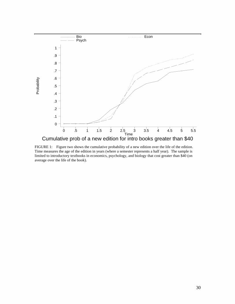
30

P

roba

bilit

y

Cumulative prob of a new edition for intro books greater than $40Time

Bio Econ Psych

0 .5 1 1.5 2 2.5 3 3.5 4 4.5 5 5.5

0

.1

.2

.3

.4

.5

.6

.7

.8

.9

1

FIGURE 1: Figure two shows the cumulative probability of a new edition over the life of the edition. Time measures the age of the edition in years (where a semester represents a half year). The sample is limited to introductory textbooks in economics, psychology, and biology that cost greater than $40 (on average over the life of the book).

31

Table 1 Mean St. Dev. Price 11464 57.69 24.13 ECON 11464 0.28 0.45 BIO 11464 0.20 0.40 INTRO 11464 0.25 0.43 AVSHRINK 11464 0.47 40.64 SPRING 11464 0.52 0.50 AVSAT 11464 1052.42 59.12 FRACREQ 11464 0.92 0.16 EDAGE 11464 2.60 3.26 PAPERBACK 11464 0.48 0.50 Fraction assignees buying book new 11464 0.30 0.18 Fraction assignees buying book overall 11464 0.50 0.18

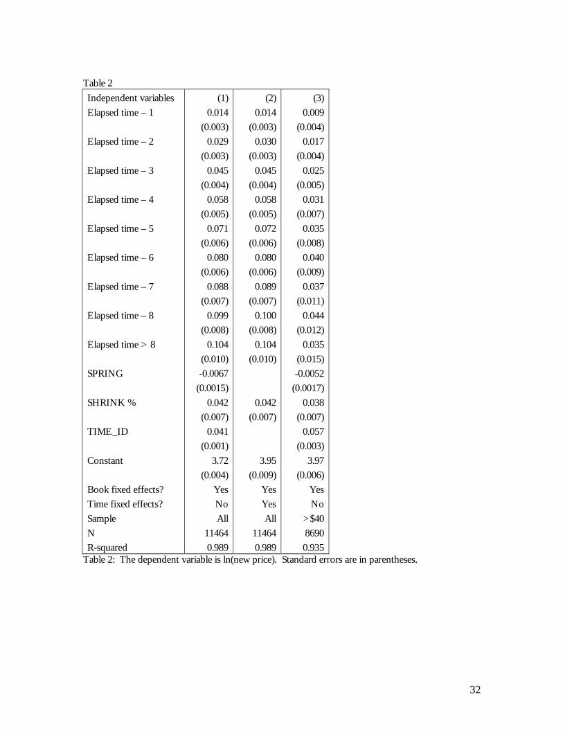
32

Table 2 Independent variables (1) (2) (3) Elapsed time – 1 0.014 0.014 0.009 (0.003) (0.003) (0.004) Elapsed time – 2 0.029 0.030 0.017 (0.003) (0.003) (0.004) Elapsed time – 3 0.045 0.045 0.025 (0.004) (0.004) (0.005) Elapsed time – 4 0.058 0.058 0.031 (0.005) (0.005) (0.007) Elapsed time – 5 0.071 0.072 0.035 (0.006) (0.006) (0.008) Elapsed time – 6 0.080 0.080 0.040 (0.006) (0.006) (0.009) Elapsed time – 7 0.088 0.089 0.037 (0.007) (0.007) (0.011) Elapsed time – 8 0.099 0.100 0.044 (0.008) (0.008) (0.012) Elapsed time > 8 0.104 0.104 0.035 (0.010) (0.010) (0.015) SPRING -0.0067 -0.0052 (0.0015) (0.0017) SHRINK % 0.042 0.042 0.038 (0.007) (0.007) (0.007) TIME_ID 0.041 0.057 (0.001) (0.003) Constant 3.72 3.95 3.97 (0.004) (0.009) (0.006) Book fixed effects? Yes Yes Yes Time fixed effects? No Yes No Sample All All >$40 N 11464 11464 8690 R-squared 0.989 0.989 0.935

Table 2: The dependent variable is ln(new price). Standard errors are in parentheses.

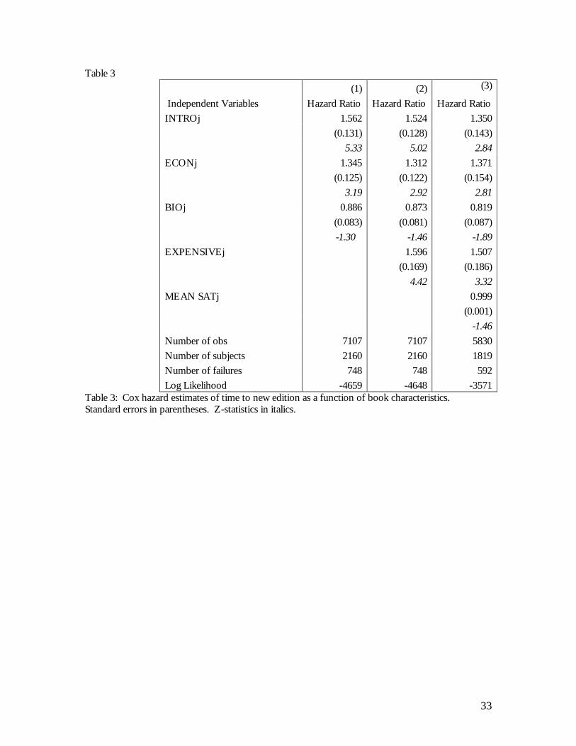
33

Table 3 (1) (2) (3)

Independent Variables Hazard Ratio Hazard Ratio Hazard Ratio INTROj 1.562 1.524 1.350 (0.131) (0.128) (0.143) 5.33 5.02 2.84 ECONj 1.345 1.312 1.371 (0.125) (0.122) (0.154) 3.19 2.92 2.81 BIOj 0.886 0.873 0.819 (0.083) (0.081) (0.087) -1.30 -1.46 -1.89 EXPENSIVEj 1.596 1.507 (0.169) (0.186) 4.42 3.32 MEAN SATj 0.999 (0.001) -1.46 Number of obs 7107 7107 5830 Number of subjects 2160 2160 1819 Number of failures 748 748 592 Log Likelihood -4659 -4648 -3571

Table 3: Cox hazard estimates of time to new edition as a function of book characteristics. Standard errors in parentheses. Z-statistics in italics.

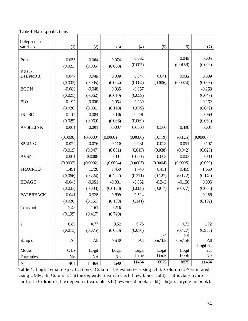
34

Table 4: Basic specifications

Independent variables

(1) (2) (3)

(4)

(5)

(6)

(7)

Price -0.053 -0.064 -0.074 -0.062 -0.045 -0.005

(0.023) (0.005) (0.008) (0.005) (0.0188) (0.003) P x (1-DIEPROB) 0.047 0.049 0.039 0.047 0.041 0.032 0.009 (0.002) (0.005) (0.004) (0.004) (0.006) (0.0074) (0.003) ECON -0.080 -0.048 0.035 -0.057 -0.258 (0.023) (0.062) (0.010) (0.059) (0.049) BIO -0.192 -0.038 0.054 -0.039 -0.162 (0.028) (0.081) (0.110) (0.079) (0.049) INTRO -0.119 -0.084 -0.046 -0.091 -0.069 (0.025) (0.069) (0.086) (0.069) (0.039) AVSHRINK 0.001 0.001 0.0007 0.0008 0.360 0.498 0.001

(0.0000) (0.0000) (0.0000) (0.0000) (0.119) (0.125)

(0.0000)

SPRING -0.079 -0.076 -0.110 -0.081 -0.023 -0.051 -0.197 (0.019) (0.047) (0.051) (0.045) (0.038) (0.042) (0.028) AVSAT 0.001 0.0008 0.001 0.0006 0.003 0.003 0.000 (0.0002) (0.0002) (0.0004) (0.0003) (0.0004) (0.0005) (0.000) FRACREQ 1.491 1.728 1.459 1.743 0.431 0.469 1.669 (0.066) (0.224) (0.222) (0.211) (0.127) (0.122) (0.140) EDAGE -0.043 -0.051 -0.081 -0.052 -0.343 -0.150 0.005 (0.003) (0.008) (0.0128) (0.008) (0.017) (0.077) (0.005) PAPERBACK -0.041 -0.328 -0.609 -0.324 0.186 (0.026) (0.151) (0.188) (0.141) (0.109) Constant -2.42 -1.61 -0.216 (0.199) (0.417) (0.729)

? 0.89 0.77 0.52

0.76

0.72

1.72 (0.013) (0.075) (0.083) (0.070) (0.427) (0.956)

Sample All All >$40

All >4

obs/bk >4

obs/bk

All

Model OLS Logit Logit

Logit

Logit

Logit Logit-alt

rat Dummies? No No No Time Book Book No

N 11464 11464 8690 11464 8875 8875 11464

Table 4: Logit demand specifications. Column 1 is estimated using OLS. Columns 2-7 estimated using GMM. In Columns 1-6 the dependent variable is ln(new books sold) – ln(no. buying no book). In Column 7, the dependent variable is ln(new+used books sold) – ln(no. buying no book).

35

Table 5: Robustness to alternative specifications of E(Price).

Independent variables

(1) (2) (3)

(4)

Price -0.059 -0.048 -0.042

(0.005) (0.004) (0.004)

Px(1-0.8*DIEPROB) 0.047

(0.005)

Price x (No revision) 0.038 0.036

(0.003) (0.003)

P x (Age<2) -0.013

(0.005)

P x (2<Age<3) -0.022

(0.005)

P x (Age>3) -0.015

(0.068)

? 0.80 0.80

0.86 (0.088) (0.096) (0.106)

Sample All All All before

2001 All before

2001

Model Logit Logit Logit

Logit Instruments for actual hazard - -

Estimated hazard

Age dummies

N 11464 11464 9297 9297 Table 5: Logit demand specifications. The dependent variable is ln(new books sold) – ln(no. buying no book); all specifications are estimated using GMM. All explanatory variables from Table 4 are included, but coefficients only from the variables of interest are reported.

36

Table 6: Robustness to alternative explanations/ continuous book heterogeneity measures

Independent variables

(1) (2) (3)

(4)

Price -0.069 -.055 -0.066 -0.067

(0.012) (0.006) (0.004) (0.004)

Price x

(Edition Age) 0.0008

(0.002)

(Past asg/Current asg) -0.0004

(0.0001)

(SAT – mean SAT) 0.00004

(0.00005)

(Commuter – mean Com) -0.0005

(0.0003)

P x (1-DIEPROB) 0.053 0.043 0.047 0.046

(0.009) (0.004) (0.004) (0.004)

P x (1-DIEPROB) x

(SAT – mean SAT) 0.00005

(0.00006)

(Commuter – mean Com) 0.0003

(0.0003)

? 0.77 0.78 0.72

0.69

(0.073) (0.077) (0.06)

(0.06)

Model Logit Logit Logit

Logit N 11464 11464 11464 11464

Table 6: Logit demand specifications. The dependent variable is ln(new books sold) – ln(no. buying no book); all specifications are estimated using GMM. Also included in the specifications are the same set of explanatory variables as in Table 4, although coefficients are omitted above for space.

37

TABLE 7: Discrete type models (1)

(2)

(3a)

Keepers (3b)

Sellers

Intro(1)

Adv(2)

Econ(1)

Psych(2)

Bio(3)

New Price

P*(1-DIE)

New Price

P*(1-DIE)

New Price

P*(1-DIE)

New Price

P*(1-DIE)

New Price

P*(1-DIE)

New Price

P*(1-DIE)

?1

?2

?3

Dummies

Model

Sample

N

-0.032 (0.012) 0.043

(0.007)

-0.077 (0.008) 0.068

(0.010)

1.330 ( 0.483) 0.885

(0.071)

No

Logit

All

11,464

-0.042 (0.007) 0.0371 (0.006) -0.076 (0.005) 0.050

(0.007) -0.089 (0.012) 0.051

(0.015)

0.894 (0.124) 0.658

(0.077) 0.581

(0.118)

No

Logit

All

11,464

-0.0651 (0.005)

Book

Besanko et. al.

>4obs/bk

used data avail

7,667

-0.0651 (0.005) 0.045

(0.001)

0.70

Table 7: Columns 1 and 2 present logit demand specifications. The dependent variable is ln(new books sold) – ln(no. buying no book) and are estimated using GMM. Standard errors are clustered at the course level. Columns 3a and 3b give the results from a mixture model with two types of consumers as described in the text. All specifications include the same set of explanatory variables as in Table 4, although coefficients are omitted above for space.

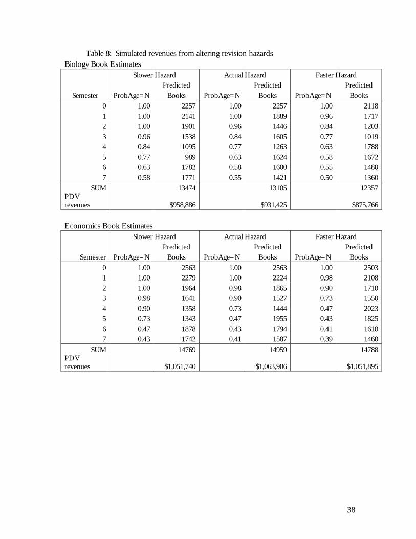
38

Table 8: Simulated revenues from altering revision hazards Biology Book Estimates Slower Hazard Actual Hazard Faster Hazard

Predicted Predicted Predicted Semester ProbAge=N Books ProbAge=N Books ProbAge=N Books

0 1.00 2257 1.00 2257 1.00 2118 1 1.00 2141 1.00 1889 0.96 1717 2 1.00 1901 0.96 1446 0.84 1203 3 0.96 1538 0.84 1605 0.77 1019 4 0.84 1095 0.77 1263 0.63 1788 5 0.77 989 0.63 1624 0.58 1672 6 0.63 1782 0.58 1600 0.55 1480 7 0.58 1771 0.55 1421 0.50 1360

SUM 13474 13105 12357 PDV revenues $958,886 $931,425 $875,766 Economics Book Estimates Slower Hazard Actual Hazard Faster Hazard

Predicted Predicted Predicted Semester ProbAge=N Books ProbAge=N Books ProbAge=N Books

0 1.00 2563 1.00 2563 1.00 2503 1 1.00 2279 1.00 2224 0.98 2108 2 1.00 1964 0.98 1865 0.90 1710 3 0.98 1641 0.90 1527 0.73 1550 4 0.90 1358 0.73 1444 0.47 2023 5 0.73 1343 0.47 1955 0.43 1825 6 0.47 1878 0.43 1794 0.41 1610 7 0.43 1742 0.41 1587 0.39 1460

SUM 14769 14959 14788 PDV revenues $1,051,740 $1,063,906 $1,051,895

39

Bibliography Akerlof, G. (1970), “The Market for ‘Lemons: Quality Uncertainty and the Market Mechanism," Quarterly Journal of Economics, 84(3), 488-500. Barro, R. (1972), “Monopoly and Contrived Depreciation,” Journal of Political Economy 80, 598-602. Berry, S. (1994), “Estimating discrete-choice models of product differentiation”, Rand Journal of Economics 25, 242-62. Berry, S., Carnall, M., and Spiller, P. (1997), “Airline Hubs: Costs, Markups, and the Implications of Consumer Heterogeneity,” working paper, Yale University. Berry, S., Levinsohn, J. and Pakes, A., (1995), “Automotive Prices in Market Equilibrium,” Econometrica 63, 841-890. Besanko, D., Dube, J. and Gupta, S. (2003), “Competitive Price Discrimination Strategies in a Vertical Channel”, Management Science 49, 1121-1138. Bulow, J. (1982), “Durable Goods Monopolists,” Journal of Political Economy 90, 314-332. Bulow, J. (1986), “An Economic Theory of Planned Obsolescence”, Quarterly Journal of Economics 101(4), 729-749.

Caballero, R. (1990), “Expenditure on Durable Goods: A Case for Slow Adjustment,” Quarterly Journal of Economics 422(3), 727-744. Caballero, R. (1993), “Durable Goods: An Explanation for their Slow Adjustment,” Journal of Political Economy 101(2), 351-384.

Carlton, D. and Gertner, R. (1989), "Market Power and Mergers in Durable-Good Industries," Journal of Law & Economics 32(2), S203-26.

Carranza, J.E., (2004), “An Empirical Model of Endogenous Quality Formation in Durable Goods Markets,” Yale University working paper.

40

Coase, R. (1972), 'Durability and Monopoly', Journal of Law and Economics 15(1), p. 143-149.

Copeland, A. and J. Stevens (2004), “The substitutability of new and used goods: highway rollers”, Federal Reserve Board Working Paper (2004). Dorans (1999), http://www.collegeboard.com/repository/rr9901_3913.pdf, page 17. Eberly, J. (1994), "Adjustment of Consumers' Durables Stocks: Evidence from Automobile Purchases," Journal of Political Economy. Ellison, S., I. Cockburn, Z. Griliches, J. Hausman (1997) , “Characteristics of demand for pharmaceutical products: The case of four cephalosporins,” Rand Journal of Economics 28, Autumn 1997. Esteban, S. and M. Shum (2004), “Durable-goods oligopoly with secondary markets: the case of automobiles,” Johns Hopkins University Working Paper. Fairchild, M. (2004), “Ripoff 101: How the current practices of the textbook industry drive up the cost of college textbooks,” Calpirg Report, http://calpirg.org/reports/textbookripoff.pdf. Fang, H. and D. Silverman (2002), “Time-Inconsistency and Welfare Program Participation: Evidence from the NLSY”, April 2002. Frederick, Shane, George Lowenstein, and Ted O'Donoghue, "Time-Discounting and Time Preference: A Critical Review," Journal of Economic Literature, XL (June), pp. 351-401. Friedman, Milton (1962), Price Theory, Aldine (Chicago, Illinois). Fudenberg, D. and Tirole, J. (1998) “Upgrades, Tradeins, and Buybacks,” Rand Journal of Economics 29 (2), 235-258. Gabaix, X. and D. Laibson (2005), “Shrouded Attributes, Consumer Myopia, and Information Suppression in Competitive Markets”, MIT Working Paper. Galbraith, John K. (1958), The Affluent Society, Houghton Mifflin.

41

Goolsbee, Austan and Amil Petrin, "The Consumer Gains from Direct Broadcast Satellites and the Competition with Cable Television," Econometrica 72(2), March 2004, 351-381. Gul, F., Sonnenschein, H., and Wilson, R., “Foundations of Dynamic Monopoly and the Coase Conjecture,” Journal of Economic Theory 39, 155-190. Iiuzuka, T. (2004) “An Empirical Analysis of Planned Obsolescence,” Vanderbilt Working Paper. Laibson, D. (1997) “Golden Eggs and Hyperbolic Discounting”, Quarterly Journal of Economics 112, 443-477. Laibson, D., A. Repetto, and J. Tobacman (2004), “Estimating Discount Functions from Lifecycle Consumption Choices”, Harvard University working paper. Levinthal, D. and D. Purohit (1989), “Durable Goods and Product Obsolescence,” Marketing Science 8 (1), 35-56. McClure, S.M., D.I. Laibson, G. Loewenstein, and J.B. Cohen (2004), “Separate Neural Systems Value Immediate and Delayed Monetary Rewards”, Science 306, 503-507. Melnikov, O. (2000), “Demand for Differentiated Durable Goods: The Case of the US Computer Printer Market,” Yale University working paper. Miller, H.L. (1974), “On Killing the Market for Used Textbooks and the Relationship Between Markets for New and Secondhand Goods.” Journal of Political Economy 82, 612-619. Nasar, S. (2002), “Readers As Salesmen,” New York Times 4/17/2002, p. 23. National Association of College Stores (2004), “Frequently Asked Questions about Used Books”, http://www.nacs.org/common/research/ faq_usedbooks.pdf Nocke, V. and Peitz, M. (2002), “Hyperbolic Discounting and Secondary Markets”, University of Pennsylvania working paper. Paserman, D. (2002), “Job Search and Hyperbolic Discounting: Structural Estimation and Policy Evaluation”, Hebrew University working paper.

42

Rust, J. (1986) “When is it optimal to kill off the market for used durable goods?” Econometrica 54,65-86. Schumer, C. (2004), “Press release”, http://schumer.senate.gov/SchumerWebsite/ pressroom/press_releases/PR02384.html.

Sieper, E. and Swan, P.L. (1974), “Monopoly and Competition in the market for durable goods.” Review of Economic Studies 40, p. 333-351. Stokey, N. (1981), “Rational Expectations and Durable Goods Pricing”, Bell Journal of Economics 12, 112-128. Suslow, V. (1986), “Estimating Monopoly Behavior with Competitive Recycling: An Application to Alcoa,” The Rand Journal of Economics, 17(3), 389. Swan, P.L. (1970), “Durability of Consumption Goods.” American Economic Review 60, 884-894. Swan, P.L. (1971), “The Durability of Goods and Regulation of Monopoly,” Bell Journal of Econmics 2, 347-357.

Swan, P. L. (1980), “Alcoa: The Influence of Recycling on Monopoly Power,” The Journal of Political Economy, 88(1), 76–99. Viard, B. (2004), “Information Good Upgrades: Theory and Evidence,” Stanford University Working Paper. Waldman, M. (1993), “A New Perspective on Product Obsolescence.” Quarterly Journal of Economics 108, 273-283.

Waldman, M. (2003),Durable Goods Theory for Real World Markets, Journal of Economic Perspectives 17, No. 1, Winter 2003, pages 131-154.